1 Introduction
Bubbles are involved in a variety of processes, from bread and cheese making (Campbell & Mougeot Reference Campbell and Mougeot1999) to the fabrication of frost-resistant concrete (Hover Reference Hover1993). Bubble vibrations are associated with acoustic emissions responsible for a wide range of sounds including those of flowing water and rain (Minnaert Reference Minnaert1933; Prosperetti, Crum & Pumphrey Reference Prosperetti, Crum and Pumphrey1989) or volcanoes (Vidal et al. Reference Vidal, Ripepe, Divoux, Legrand, Géminard and Melo2010) but their ability to interact with sound also allows diverse applications such as ultrasonic imaging (Becher & Burns Reference Becher and Burns2000) or phonic insulation (Leroy et al. Reference Leroy, Bretagne, Fink, Willaime, Tabeling and Tourin2009). But bubbles can be also harmful, and their fast collapse can result in severe damage to nearby materials (Lauterborn & Kurz Reference Lauterborn and Kurz2010), causing erosion at the surface of boat propellers (Brennen Reference Brennen1995) or knocking out prey when cavitation bubbles are emitted by the fast closure of the claws of pistol shrimps (Versluis et al. Reference Versluis, Schmitz, von der Heydt and Lohse2000).
The wide range of contexts where bubbles are involved has led to a number of investigations, from the early work of Minnaert on musical air bubbles (Minnaert Reference Minnaert1933) to recent applications in medicine (Hsiao et al. Reference Hsiao, Choi, Singh, Chahine, Hay, Ilinskii, Zabolotskaya, Hamilton, Sankin and Yuan2013; Ohl et al. Reference Ohl, Tandiono, Klaseboer, Ow, Choo and Ohl2015). Minnaert’s work, as well as the derivation of the well-known Rayleigh–Plesset equation (Rayleigh Reference Rayleigh1917; Plesset Reference Plesset1949), considered bubbles in extended liquids; Strasberg (Reference Strasberg1953) calculated the shift in the natural oscillation frequency of a bubble induced by a nearby flat wall, and other types of confinement have been studied since, particularly bubbles in cylindrical tubes (Og̃uz & Prosperetti Reference Og̃uz and Prosperetti1998; Martynov, Stride & Saffari Reference Martynov, Stride and Saffari2009). Typically, the proximity of a confining solid surface increases the effective inertia during bubble oscillations, thus decreasing the oscillation frequency, but increases of the oscillation frequency are also expected when close to soft or free surfaces (Strasberg Reference Strasberg1953; Martynov et al. Reference Martynov, Stride and Saffari2009). Striking non-spherical deformations of oscillating bubbles due to interactions with walls have also been demonstrated close to solid surfaces (Lauterborn & Ohl Reference Lauterborn and Ohl1997) or in microfluidic cavitation experiments (Zwaan et al. Reference Zwaan, Le Gac, Tsuji and Ohl2007).
Bubble dynamics in fully confined situations, however, has received little attention. We define a situation as fully confined if the liquid containing the bubbles is surrounded by walls in all directions of space, so that no flux in or out of the confining material is possible. The condition of full confinement thus also holds for situations where fluxes are possible in and out of the confining cavity (e.g. porous walls), if the typical time scale of these fluxes is large compared to the time scales of interest for the bubble dynamics. In unconfined or partially confined situations, bubble volumetric deformations can be accommodated by pushing the liquid away. This is no longer true in a fully confined situation, where any expansion of the bubble must be accompanied by compression of the liquid and/or stretching of the surrounding material.
If this situation of full confinement seems extreme, it occurs frequently in nature and in technology. Rocks contain trapped fluid inclusions and the study of the quasi-static behaviour of bubbles in these inclusions is used by geologists to extract past thermodynamic conditions (Roedder and Bodnar Reference Roedder and Bodnar1980; Marti et al. Reference Marti, Krüger, Fleitmann, Frenz and Rička2012). Impact of projectiles into liquid-filled tanks can generate cavitation bubbles with disastrous consequences for the solid structure (Fourest et al. Reference Fourest, Laurens, Deletombe, Dupas and Arrigoni2015). Water status in plants or in soils is also typically measured by tensiometers where an isolated pocket of liquid is put in equilibrium with the material and the unwanted appearance of bubbles can disrupt the function of these devices (Tarantino & Mongiovì Reference Tarantino, Mongiovì and Toll2001; Pagay et al. Reference Pagay, Santiago, Sessoms, Huber, Vincent, Pharkya, Corso, Lakso and Stroock2014). Plants contain fluid-filled vessels (xylem) to transport the water from the roots to the leaves and the growth of bubbles in xylem is a cause of mortality during drought (Tyree & Sperry Reference Tyree and Sperry1989; Cochard Reference Cochard2006). Another striking example of confined bubble dynamics in plants is the cavitation-based mechanism of ejection of spores in some species of ferns (Noblin et al. Reference Noblin, Rojas, Westbrook, Llorens, Argentina and Dumais2012). Cavitation bubbles have also been shown to appear during the peeling of adhesives (Poivet et al. Reference Poivet, Nallet, Gay and Fabre2003), the curing of cement (Lura et al. Reference Lura, Couch, Jensen and Weiss2009) or the drying of porous media (Vincent et al. Reference Vincent, Sessoms, Huber, Guioth and Stroock2014b ), i.e. many situations where the liquid can be effectively fully confined.
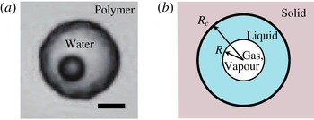
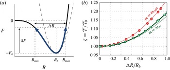
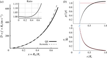
The recent development of transparent platforms with pockets of liquid confined in porous solids (Wheeler & Stroock Reference Wheeler and Stroock2008; Vincent et al. Reference Vincent, Sessoms, Huber, Guioth and Stroock2014b ) allowed experimental investigations of bubble dynamics in fully confined situations with controlled geometries (figure 1 a). These experiments demonstrated an order-of-magnitude increase in the frequency of bubble oscillations, unusually quick damping of the oscillations, as well as rich non-radial bubble instabilities (Vincent et al. Reference Vincent, Marmottant, Gonzalez-Avila, Ando and Ohl2014a ). Here we propose a complete, detailed and general theory to describe bubble statics and dynamics in full confinement.
The paper is organized as follows.
-
(i) In § 2, we examine the statics of a fully confined bubble by deriving its potential energy with respect to radial deformations, taking into account the effects of gas compressibility, surface tension, liquid compressibility and solid elasticity. We discuss the implications for bubble stability in confinement and establish a phase diagram that predicts bubble superstability and modifications in the Blake threshold.
-
(ii) In § 3, we calculate the velocity field and associated kinetic energy (setting the effective mass for the dynamics) for radial bubble deformations in full confinement, taking into account the liquid compressibility and the solid deformations.
-
(iii) In § 4, we combine the results from §§ 2.1 (potential energy) and 3 (kinetic energy) to establish the complete dynamics of fully confined bubbles, including modified Minnaert and Rayleigh–Plesset equations. We also discuss the relative importance of dissipation mechanisms (viscous, acoustic, thermal).
-
(iv) In a last section, § 5, we discuss the results from the previous sections with respect to existing models (§ 5.1) and experimental results (§ 5.2), the hypotheses of our model (§§ 5.3–5.5) and the general stability predictions from the statics analysis (§§ 5.6 and 5.7).
(a) Bubble in a spherical pocket of liquid confined in a stiff polymer hydrogel (adapted from Vincent et al. (Reference Vincent, Marmottant, Gonzalez-Avila, Ando and Ohl2014a
)). Scale bar is
 $20~\unicode[STIX]{x03BC}\text{m}$
. Despite being porous, the hydrogel creates an effective confinement for the liquid because time scales for water diffusion in the gel are much longer than the bubble dynamics (Vincent et al.
Reference Vincent, Marmottant, Quinto-Su and Ohl2012). (b) Here, we consider a spherical bubble in a liquid-filled spherical cavity embedded in a solid. We discuss different shapes for the solid, including an infinitely extended one as sketched here, and thin shells (see text).

1.1 Framework, hypotheses and definitions
We consider a spherical bubble of radius
 $R$
in a liquid; the liquid and the bubble are confined in a spherical cavity of radius
 $R_{c}$
within a solid (figure 1
b). This three-layer geometry (bubble–liquid–solid) has similarities with previous studies that have considered bubble–liquid–air (Obreschkow et al.
Reference Obreschkow, Kobel, Dorsaz, de Bosset, Nicollier and Farhat2006), bubble–solid shell–liquid (Church Reference Church1995) or bubble–liquid–solid shell (Fourest et al.
Reference Fourest, Laurens, Deletombe, Dupas and Arrigoni2015). The case of Fourest et al. (Reference Fourest, Laurens, Deletombe, Dupas and Arrigoni2015) is closest to the case considered here, however, these authors considered a situation where the liquid is incompressible and all variations of bubble volume were accommodated by modifications of the shell radius. Here, we consider a more general situation where both the liquid volume and the cavity size may vary, and where the confinement geometry can be an extended elastic solid or an elastic shell.
For the kinematics and dynamics calculations (§§ 3–4), we will make the simplifying assumption that the bubble is centred in the cavity, and we discuss possible corrections in § 5.3. This assumption is not necessary for the potential energy and statics derivations (§ 2). We consider the system to evolve isothermally (temperature
 $T$
) so that the thermodynamic potential is the free energy
 $F$
; we discuss non-isothermal effects in § 5.5. We consider that the bubble contains the saturated vapour of the liquid (partial pressure
 $P_{sat}(T)$
) and possibly incondensable gas, later referred to as trapped gas (in practice, trapped gas is gas that is not the vapour of the liquid and whose diffusion in and out of the bubble is slow compared to the typical time scales of interest) with number of particles
 $N_{g}$
, partial pressure
 $p_{g}\times 4\unicode[STIX]{x03C0}R^{3}/3=N_{g}k_{B}T$
, with
 $k_{B}$
the Boltzmann constant from the ideal gas law. The liquid–gas interface has a surface tension
 $\unicode[STIX]{x1D70E}$
. We assume the volume of the bubble to be small compared to the volume of the cavity, i.e.
 $(R/R_{c})^{3}\ll 1$
. In practice, this means that the radius of the bubble should not be larger than typically half of that of the cavity (when
 $R/R_{c}=0.5$
,
 $(R/R_{c})^{3}=0.125$
). This will allow us to use the laws of linear elasticity for the solid and the liquid, as well as to define all deformations with respect to the reference state where
 $R=0$
. In § 5.3, we discuss how to modify the expressions in our model if a reference state different from
 $R=0$
is chosen.
In the following, to simplify the expressions and discussion, we will the define driving pressure
 $$\begin{eqnarray}\unicode[STIX]{x0394}P=P-P_{sat},\end{eqnarray}$$
where
 $P$
is the liquid pressure and
 $P_{sat}$
the saturation vapour pressure.
 $\unicode[STIX]{x0394}P$
takes account the contribution of the vapour; we will use the terms negative pressure for
 $\unicode[STIX]{x0394}P<0$
(
 $P<P_{sat}$
) and positive pressure for
 $\unicode[STIX]{x0394}P>0$
. We also define the associated critical radius
 $$\begin{eqnarray}R_{\infty }^{\ast }=-\frac{2\unicode[STIX]{x1D70E}}{\unicode[STIX]{x0394}P}\end{eqnarray}$$
at which a bubble is in unstable equilibrium at
 $\unicode[STIX]{x0394}P$
(Brennen Reference Brennen1995).
2 Potential energy and statics
In this section, we evaluate the potential energy
 $F$
in full confinement as a function of the bubble radius
 $R$
, and discuss the equilibrium solutions for
 $R$
, i.e. the values of
 $R$
that are extrema of
 $F(R)$
. As mentioned in § 1, expanding a bubble in full confinement requires compression of the liquid surrounding the bubble and/or deformation of the solid encapsulating the liquid. As a result, liquid compressibility and solid elasticity are key ingredients in the calculations below.
2.1 Free energy of a fully confined bubble
The contributions to the total free energy
 $F(R)$
of both the liquid–gas interface
 $F_{\unicode[STIX]{x1D70E}}$
and the trapped gas
 $F_{g}$
are related respectively to the excess energy due to surface tension associated with changes of the interface area and the work of the gas pressure
 $p_{g}$
associated with isothermal changes of the bubble volume:
 $$\begin{eqnarray}\displaystyle & \displaystyle F_{\unicode[STIX]{x1D70E}}(R)=4\unicode[STIX]{x03C0}R^{2}\unicode[STIX]{x1D70E}, & \displaystyle\end{eqnarray}$$
 $$\begin{eqnarray}\displaystyle & \displaystyle F_{g}(R)=-3N_{g}k_{B}T\ln \left(\frac{R}{R_{ref}}\right), & \displaystyle\end{eqnarray}$$
where
 $R_{ref}$
is an arbitrary radius. The expressions for
 $F_{\unicode[STIX]{x1D70E}}$
and
 $F_{g}$
are identical to cases without confinement.
In order to calculate the liquid and solid contributions, we evaluate how the pressure
 $\unicode[STIX]{x0394}P$
relates to the bubble growth (bubble volume
 $V=4\unicode[STIX]{x03C0}R^{3}/3$
). We assume that the number
 $N_{\ell }$
of liquid molecules is constant (neglecting the loss due to evaporation/condensation). The relation between liquid pressure
 $P$
and liquid volume
 $V_{\ell }$
thus follows the liquid equation of state
 $P(V_{\ell })$
at a constant number of particles, which can be linearized in the form
 $$\begin{eqnarray}P=P_{0}-K_{\ell }\frac{V_{\ell }-V_{0}}{V_{0}},\end{eqnarray}$$
with a reference state
 $(P_{0},V_{0})$
and the isothermal bulk modulus
 $$\begin{eqnarray}K_{\ell }=-V_{\ell }\left(\frac{\unicode[STIX]{x2202}P}{\unicode[STIX]{x2202}V_{\ell }}\right)_{T,N_{\ell }}\end{eqnarray}$$
of the order of
 $2.2~\text{GPa}$
for water (Kell Reference Kell1975). The linearized equation of state (2.3) is valid when the typical pressure variations are small compared to
 $K_{\ell }$
. We choose the state with no bubble as reference, for which the liquid occupies the whole volume of the confinement. Then
 $V_{0}=4\unicode[STIX]{x03C0}R_{c}^{3}/3$
(where
 $R_{c}$
is the confinement radius in the reference state) and
 $P_{0}$
is the liquid pressure in the reference state (for
 $R=0$
).
If confinement is not infinitely rigid, the growth of the bubble not only compresses the liquid but also makes the confinement expand (volume
 $V_{c}>V_{0}$
). Under the assumption of small deformations, we assume that there is a linear relationship between
 $P$
and
 $V_{c}$
 $$\begin{eqnarray}P=P_{0}+K_{c}\left(\frac{V_{c}-V_{0}}{V_{0}}\right),\end{eqnarray}$$
where we have defined an effective modulus of the solid confinement
 $$\begin{eqnarray}K_{c}=V_{c}\left(\frac{\unicode[STIX]{x2202}P}{\unicode[STIX]{x2202}V_{c}}\right)_{T}.\end{eqnarray}$$
Note the opposite sign compared to the bulk modulus of the liquid (2.4), which allows us to keep these coefficients positive. The value of
 $K_{c}$
depends on the properties of the solid. For a spherical confinement in an extended, uniform and isotropic solid following the laws of linear elasticity,
 $$\begin{eqnarray}K_{c}={\textstyle \frac{4}{3}}G,\end{eqnarray}$$
where
 $G$
is the shear modulus of the solid (Landau & Lifshitz Reference Landau and Lifshitz1986). The parameter
 $K_{c}$
allows us to take into account other confinement geometries, such as solid shells of thickness
 $d$
(Fourest et al.
Reference Fourest, Laurens, Deletombe, Dupas and Arrigoni2015). In the case of thin shells this parameters is
 $K_{c}=(4/3)G(1+\unicode[STIX]{x1D708}/1-\unicode[STIX]{x1D708})(d/R_{c})$
, where
 $\unicode[STIX]{x1D708}$
is the Poisson ratio of the solid (Marmottant et al.
Reference Marmottant, Bouakaz, de Jong and Quilliet2011). Using both equations (2.3) and (2.5) as well as the fact that
 $V_{c}=V+V_{\ell }$
, we eventually find for the evolution of
 $\unicode[STIX]{x0394}P=P-P_{sat}$
 $$\begin{eqnarray}\unicode[STIX]{x0394}P=\unicode[STIX]{x0394}P_{0}+K\left(\frac{V}{V_{0}}\right)=\unicode[STIX]{x0394}P_{0}+K\left(\frac{R}{R_{c}}\right)^{3},\end{eqnarray}$$
where we have defined the effective modulus
 $$\begin{eqnarray}K=\frac{K_{\ell }K_{c}}{K_{\ell }+K_{c}},\end{eqnarray}$$
which is the harmonic average of the liquid compression modulus
 $K_{\ell }$
and of the effective confinement modulus
 $K_{c}$
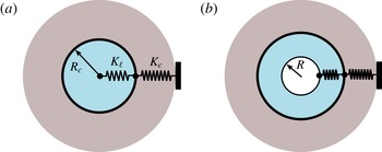
. This association is analogous to springs in series, with one formed by the liquid compressibility and the other by the solid elasticity (see figure 2). The case of a rigid confinement is obtained when
 $K_{c}\gg K_{\ell }$
, giving
 $K\simeq K_{\ell }$
. Inversely, for a confinement much more compressible than the liquid itself,
 $K\simeq K_{c}$
. In § 5.3, we discuss how to modify the expressions above if a reference state different from
 $R=0$
is chosen.
Expanding a bubble from
 $R=0$
(a) to
 $R>0$
(b) in a fully confined environment requires us to compress the liquid (compression modulus
 $K_{\ell }$
) and/or expand the confinement size by deforming the surrounding solid (effective modulus
 $K_{c}$
). The system behaves as if the two moduli
 $K_{\ell }$
and
 $K_{c}$
corresponded to stiffness of springs mounted in series (see (2.9)).

The contribution to the potential energy of the liquid (and its vapour, see discussion in the previous subsection) and of confinement elasticity is obtained by integrating
 $\int _{0}^{V}\unicode[STIX]{x0394}P(V^{\prime })\,\text{d}V^{\prime }$
using (2.8). Adding the contributions of the bubble interface and of trapped gas (equations (2.1) and (2.2)), we finally establish the total free energy
 $$\begin{eqnarray}F=\frac{4}{3}\unicode[STIX]{x03C0}R^{3}\unicode[STIX]{x0394}P_{0}\left(1+\frac{1}{2}\frac{K}{\unicode[STIX]{x0394}P_{0}}\left(\frac{R}{R_{c}}\right)^{3}\right)+4\unicode[STIX]{x03C0}R^{2}\unicode[STIX]{x1D70E}-3N_{g}k_{B}T\ln \left(\frac{R}{R_{ref}}\right),\end{eqnarray}$$
or, in dimensionless form,
 $$\begin{eqnarray}F=F^{\ast }\left[-2X^{3}\left(1-\frac{\unicode[STIX]{x1D6FE}}{2}X^{3}\right)+3X^{2}-6\unicode[STIX]{x1D6FC}\ln X\right],\end{eqnarray}$$
where
 $X=R/R^{\ast }$
is a dimensionless radius normalized with
 $$\begin{eqnarray}R^{\ast }=-2\unicode[STIX]{x1D70E}/\unicode[STIX]{x0394}P_{0},\end{eqnarray}$$
which is the critical radius that would be associated with the pressure
 $\unicode[STIX]{x0394}P_{0}$
in an unconfined situation (see (1.2)) and
 $F^{\ast }=(4/3)\unicode[STIX]{x03C0}R^{\ast 2}\unicode[STIX]{x1D70E}$
is a typical free energy (corresponding to the energy barrier for nucleation in the context of unconfined cavitation, see Brennen (Reference Brennen1995)). We have also chosen
 $R_{ref}=R^{\ast }$
. Equation (2.11) is governed by two dimensionless parameters
 $\unicode[STIX]{x1D6FC}$
and
 $\unicode[STIX]{x1D6FE}$
defined in the following manner:
 $$\begin{eqnarray}\displaystyle & \displaystyle \unicode[STIX]{x1D6FC}=\frac{\frac{3}{2}N_{g}k_{B}T}{4\unicode[STIX]{x03C0}\unicode[STIX]{x1D70E}R^{\ast 2}}, & \displaystyle\end{eqnarray}$$
 $$\begin{eqnarray}\displaystyle & \displaystyle \unicode[STIX]{x1D6FE}=\left(\frac{K_{\ell }}{-\unicode[STIX]{x0394}P_{0}}\right)\left(\frac{R^{\ast }}{R_{c}}\right)^{3}. & \displaystyle\end{eqnarray}$$
These parameters represent the effect of trapped gas and the effect of confinement, respectively. Using the expression of the critical radius
 $R^{\ast }$
(2.12), these parameters can be rewritten
 $$\begin{eqnarray}\displaystyle & \displaystyle \unicode[STIX]{x1D6FC}=\frac{3N_{g}k_{B}T\unicode[STIX]{x0394}P_{0}^{2}}{32\unicode[STIX]{x03C0}\unicode[STIX]{x1D70E}^{3}}, & \displaystyle\end{eqnarray}$$
 $$\begin{eqnarray}\displaystyle & \displaystyle \unicode[STIX]{x1D6FE}=\frac{8\unicode[STIX]{x1D70E}^{3}K}{R_{c}^{3}\unicode[STIX]{x0394}P_{0}^{4}}. & \displaystyle\end{eqnarray}$$
The corresponding equilibrium solutions follow
 $(\text{d}F/\text{d}R)_{R=R_{eq}}=0$
, leading to
 $$\begin{eqnarray}\unicode[STIX]{x0394}P_{0}+K\left(\frac{R_{eq}}{R_{c}}\right)^{3}+\frac{2\unicode[STIX]{x1D70E}}{R_{eq}}-p_{g,eq}=0,\end{eqnarray}$$
where
 $p_{g,eq}$
is the equilibrium pressure of trapped gas in the bubble following
 $p_{g,eq}\times (4/3)\unicode[STIX]{x03C0}R_{eq}^{3}=N_{g}k_{B}T$
. Equation (2.17) corresponds to the Laplace equation since from (2.8),
 $\unicode[STIX]{x0394}P_{0}+K(R_{eq}/R_{c})^{3}$
is the pressure in the liquid (corrected by
 $P_{sat}$
) when the bubble has a radius
 $R_{eq}$
. The equivalent dimensionless equilibrium equation is
 $$\begin{eqnarray}\unicode[STIX]{x1D6FE}X_{eq}^{2}(X_{eq}^{3}-1)+X_{eq}-\frac{\unicode[STIX]{x1D6FC}}{X_{eq}}=0,\end{eqnarray}$$
where
 $X_{eq}=R_{eq}/R^{\ast }$
.
Note that both parameters
 $\unicode[STIX]{x1D6FC}$
and
 $\unicode[STIX]{x1D6FE}$
are always positive, but the value of
 $R^{\ast }$
can be either positive or negative depending on the value of
 $\unicode[STIX]{x0394}P_{0}$
. In cases where
 $R^{\ast }<0$
(
 $\unicode[STIX]{x0394}P_{0}>0$
, i.e.
 $P_{0}>P_{sat}$
) there is only one equilibrium radius which is
 $R=0$
if
 $\unicode[STIX]{x1D6FC}=0$
and a non-zero value if there is trapped gas. In the following, we will focus on the more interesting situation
 $\unicode[STIX]{x0394}P_{0}<0$
(liquid at negative pressure, or
 $P_{0}<P_{sat}$
), in other words consider only the zone where
 $R/R^{\ast }>0$
in the potential energy landscape.
We also remark that
 $\unicode[STIX]{x0394}P_{0}$
identifies with the pressure in the liquid prior to nucleation in a cavitation context, but does not correspond to the ambient liquid pressure
 $\unicode[STIX]{x0394}P$
for static, pre-existing bubbles. In that latter case,
 $\unicode[STIX]{x0394}P_{0}$
is a reference pressure that can be calculated using (2.17) and that is typically negative even if
 $\unicode[STIX]{x0394}P>0$
, except for bubbles very small compared to the cavity size.
2.2 Phase diagram
Possible shapes of the free energy (2.11) as a function of the two dimensionless parameters
 $\unicode[STIX]{x1D6FC}$
and
 $\unicode[STIX]{x1D6FE}$
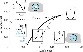
are shown in figure 3. In general, two stable positions of the bubble exist, one at small radius
 $R_{a}$
(germ) and one at higher radius
 $R_{b}$
(bubble). These two minima are separated by an energy barrier situated at the unstable equilibrium radius
 $R^{\prime }\simeq R^{\ast }$
. As can be seen in figure 3, the system behaves as a two-state system (bubble and germ) with the order parameters
 $\unicode[STIX]{x1D6FE}$
and
 $\unicode[STIX]{x1D6FC}$
controlling a first-order transition between these states. The system also exhibits a critical point (C in figure 3) where the two solutions merge to form a characteristic flat-bottom free energy curve. In the following, we discuss the main features of the phase diagram by analysing limiting cases.
Phase diagram of bubble free energy and equilibrium solutions as a function of the dimensionless parameters
 $\unicode[STIX]{x1D6FE}$
(confinement) and
 $\unicode[STIX]{x1D6FC}$
(trapped gas). Line (T) corresponds to a transition (binodal) line between two stable states: the bubble (
 $R^{b}$
) on the left and the germ (
 $R_{a}$
) on the right. The dashed lines correspond to spinodals beyond which one of the solutions disappears: (B) is the generalized Blake threshold and (S) is the superstability line. The insets show the corresponding shapes of the potential
 $F(R)$
from (2.11). Germ, bubble and the unstable equilibrium solution
 $R^{\prime }$
all merge at a critical point (C).

2.2.1 Effect of confinement: classical nucleation theory, the bubble solution and superstability
We first discuss the effect of confinement by assuming
 $\unicode[STIX]{x1D6FC}=0$
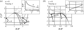
(no trapped gas). Figure 4(a) shows the shape of the free energy for increasing values of
 $\unicode[STIX]{x1D6FE}$
. The equilibrium condition
 $\text{d}F/\text{d}R=0$
with
 $\unicode[STIX]{x1D6FC}=0$
always admits a trivial solution
 $R_{a}=0$
. This solution describes a homogeneous, metastable liquid at negative pressure
 $\unicode[STIX]{x0394}P_{0}$
. Such a liquid is metastable with respect to the nucleation of bubbles (cavitation), as any bubble of size larger than
 $R^{\ast }$
grows explosively. This situation is well known and is at the basis of classical nucleation theory (CNT) to describe cavitation and boiling (Blander & Katz Reference Blander and Katz1975; Debenedetti Reference Debenedetti1996; Caupin & Herbert Reference Caupin and Herbert2006). CNT (
 $\unicode[STIX]{x1D6FE}=0$
and
 $\unicode[STIX]{x1D6FC}=0$
), however, predicts an unphysical infinite growth of cavitation bubbles (past
 $R^{\ast }$
, the potential
 $F(R)$
is continuously decreasing). As can be seen in figure 4(a), introducing
 $\unicode[STIX]{x1D6FE}\neq 0$
resolves that problem by allowing the existence of a stable solution
 $R_{b}$
, which represents the final bubble size after nucleation and growth.
For moderate confinements (
 $\unicode[STIX]{x1D6FE}\ll 1$
), one has from (2.18)
 $(R_{b}/R^{\ast })_{\unicode[STIX]{x1D6FE}\ll 1}=\unicode[STIX]{x1D6FE}^{-1/3}$
or, using (2.14)
 $$\begin{eqnarray}(R_{b})_{\unicode[STIX]{x1D6FE}\ll 1}=\left(\frac{-\unicode[STIX]{x0394}P_{0}}{K}\right)^{1/3}R_{c}.\end{eqnarray}$$
We note that formula (2.19) is still valid for non-zero values of
 $\unicode[STIX]{x1D6FC}$
if
 $\unicode[STIX]{x1D6FC}\ll 1/\unicode[STIX]{x1D6FE}$
. With the above assumption that
 $\unicode[STIX]{x1D6FE}\ll 1$
, this condition is thus not restrictive.
(a) Effect of the confinement parameter
 $\unicode[STIX]{x1D6FE}$
on the potential energy
 $F(R)$
without trapped gas (
 $\unicode[STIX]{x1D6FC}=0$
). Lighter curves correspond to higher values of
 $\unicode[STIX]{x1D6FE}$
(stronger confinement), and the following values were used: [
 $0;0.05;\unicode[STIX]{x1D6FE}_{t}=1/16;\unicode[STIX]{x1D6FE}_{s}=3^{3}/4^{4};0.2$
]. Inset: corresponding equilibrium solutions (bifurcation diagram). Continuous lines indicate stable solutions, dashed lines correspond to metastable solutions and the dotted line correspond to the unstable solution
 $R^{\prime }$
. (b) Effect of the gas parameter
 $\unicode[STIX]{x1D6FC}$
without confinement (
 $\unicode[STIX]{x1D6FE}=0$
). Lighter colours represent higher values of the dimensionless gas parameter
 $\unicode[STIX]{x1D6FC}$
(values used:
 $[0;0.05,\unicode[STIX]{x1D6FC}_{B}=4/27\,\text{(Blake threshold)},0.3]$
. Inset: bifurcation diagram.

When increasing the confinement parameter
 $\unicode[STIX]{x1D6FE}$
, the bubble solution
 $R_{b}$
gets closer to the unstable equilibrium
 $R^{\prime }\simeq R^{\ast }$
(figure 4
a), until these two solutions collapse and disappear for a value
 $\unicode[STIX]{x1D6FE}_{s}$
(figure 4
a inset). Above that point, only the homogenous liquid (
 $R=0$
) can exist. Prior reaching
 $\unicode[STIX]{x1D6FE}_{s}$
, another remarkable point is crossed: at
 $\unicode[STIX]{x1D6FE}_{t}$
, the homogeneous liquid and the bubble have the same energy. The value of
 $\unicode[STIX]{x1D6FE}_{t}$
as well as the corresponding equilibrium radius
 $R_{t}$
are found by requiring
 $\text{d}F/\text{d}R=0$
(equilibrium condition) as well as
 $F=0$
, which yields
 $$\begin{eqnarray}\displaystyle & \displaystyle \unicode[STIX]{x1D6FE}_{t}=1/16, & \displaystyle\end{eqnarray}$$
 $$\begin{eqnarray}\displaystyle & \displaystyle R_{t}/R^{\ast }=2. & \displaystyle\end{eqnarray}$$
Similarly,
 $\unicode[STIX]{x1D6FE}_{s}$
and
 $R_{s}$
are found by requiring
 $\text{d}F/\text{d}X=0$
and
 $\text{d}^{2}F/\text{d}X^{2}=0$
:
 $$\begin{eqnarray}\displaystyle & \displaystyle \unicode[STIX]{x1D6FE}_{s}=3^{3}/4^{4}, & \displaystyle\end{eqnarray}$$
 $$\begin{eqnarray}\displaystyle & \displaystyle R_{s}/R^{\ast }=4/3. & \displaystyle\end{eqnarray}$$
In other words, this result predicts that for sufficiently strong confinements, a liquid at negative pressure can become absolutely stable. We discuss implications of this surprising phenomenon of superstability in § 5 of this article. Lines (T) and (S) of the phase diagram (figure 3) respectively extend the values of
 $\unicode[STIX]{x1D6FE}_{t}$
and
 $\unicode[STIX]{x1D6FE}_{s}$
in the presence of trapped gas.
2.2.2 Effect of gas: the Blake threshold
We now discuss briefly the effect of gas by first assuming
 $\unicode[STIX]{x1D6FE}=0$
(no confinement). Figure 4(b) shows the shape of the free energy for increasing values of
 $\unicode[STIX]{x1D6FC}$
and the inset shows the corresponding equilibrium solutions found from the condition
 $\unicode[STIX]{x1D6FC}=(R/R^{\ast })^{2}\times (1-R/R^{\ast })$
from (2.18). When
 $\unicode[STIX]{x1D6FC}=0$
, the case of CNT is recovered. For
 $\unicode[STIX]{x1D6FC}>0$
, a metastable germ (
 $R_{a}$
) can exist. Increasing
 $\unicode[STIX]{x1D6FC}$
(which corresponds to an increase of the number of trapped gas particles, or to a decrease in the liquid pressure, see (2.15)) results in an increase of the germ size (see inset of figure 4), until the germ reaches a critical value
 $R_{B}=2R^{\ast }/3$
at which it becomes unstable. This situation is known as the Blake threshold from the initial work of Blake (Reference Blake1949) to describe cavitation by gaseous germs. The value of
 $R_{B}$
as well as the corresponding critical value of
 $\unicode[STIX]{x1D6FC}_{B}=4/27$
can be readily obtained by requesting
 $\text{d}F/\text{d}R=0$
and
 $\text{d}^{2}F/\text{d}R^{2}=0$
from expression (2.11).
Our dimensionless free energy approach thus allows for a grouped description of classical results of unconfined bubbles (CNT and Blake threshold) and evaluate modifications introduced by confinement. Line (B) on the phase diagram is obviously the extension of Blake threshold to fully confined situations. As can be seen from the weak slope of (B) in figure 3, the Blake threshold is not significantly affected by confinement. Beyond the critical point C, however, the generalized Blake line (B) disappears. In this particular regime of large
 $\unicode[STIX]{x1D6FE}$
(strong confinement), one thus does not observe cavitation when increasing
 $\unicode[STIX]{x1D6FC}$
, but a smooth, continuous transition from a germ to a bubble.
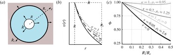
Kinematics associated with radial deformations of a spherical bubble with surface velocity
 ${\dot{R}}$
. (a) Sketch of the system. (b) Velocity field in the liquid for different values of the elastic parameter
 $\unicode[STIX]{x1D705}$
, here plotted for
 $x=R/R_{c}=0.5$
. (c) Inertia corrective factor
 $\unicode[STIX]{x1D719}$
(3.15), for various values of
 $\unicode[STIX]{x1D705}$
and for various solid densities
 $\unicode[STIX]{x1D70C}_{s}$
(assuming an extended solid), expressed here in
 $\text{kg}~\text{dm}^{-3}$
. The liquid is assumed to be water.

3 Radial kinematics and kinetic energy of fully confined bubbles
We now investigate the kinematics of fully confined bubbles by calculating the fluid and solid motion for given radial deformations of the bubble surface (figure 5 a) and the corresponding kinetic energy. Following our model hypotheses, we assume radial deformations. We also consider that bubble and cavity are centred and we will discuss possible corrections for off-centred situations in § 5.3.
A stiff confinement imposes zero velocity at the liquid–solid interface. This is possible only if the liquid is compressed during bubble growth, i.e. its average density increases, while it decreases on phases of bubble shrinkage. In order to capture this effect, we use a mean-field (or quasi-static) approximation where we consider the density
 $\unicode[STIX]{x1D70C}$
as homogeneous throughout the liquid, changing only as a function of time. We thus neglect second-order corrections associated with spatial density fluctuations. We discuss this hypotheses in § 5.4. Following this quasi-static approach, we also consider the relations obtained in the static case (§ 2) to remain valid in dynamic situations. We thus describe the natural oscillation kinematics of fully confined bubbles, but do not consider higher modes of vibration where the bubble and cavity deformations do not occur in phase.
3.1 General considerations
Within the framework discussed above, we can combine equations (2.5) and (2.8) to relate cavity deformations to bubble deformations:
 $$\begin{eqnarray}V_{c}=V_{0}+\unicode[STIX]{x1D705}V,\end{eqnarray}$$
with
 $\unicode[STIX]{x1D705}=K/K_{c}=K_{\ell }/(K_{\ell }+K_{c})$
a dimensionless elastic parameter comprised between
 $0$
and
 $1$
.
 $V_{c}=4\unicode[STIX]{x03C0}R_{c}^{3}/3$
is the confinement volume (
 $V_{0}$
is its value in the reference state without a bubble) and
 $V=4\unicode[STIX]{x03C0}R^{3}/3$
is the bubble volume. We obtain the liquid density
 $\unicode[STIX]{x1D70C}$
from the conservation of mass
 $\unicode[STIX]{x1D70C}_{0}V_{0}=\unicode[STIX]{x1D70C}(V_{c}-V)$
where
 $\unicode[STIX]{x1D70C}_{0}$
is the density in the reference state (
 $R=0$
), which translates into
 $$\begin{eqnarray}\unicode[STIX]{x1D70C}=\unicode[STIX]{x1D70C}_{0}\frac{1-\unicode[STIX]{x1D705}x^{3}}{1-x^{3}}\end{eqnarray}$$
using (3.1) and where we have defined the dimensionless variable
 $x=R/R_{c}$
. In § 5.3, we discuss how to modify the expressions above if a reference state different from
 $R=0$
is chosen. Differentiation of (3.1) also yields the useful relation
 $$\begin{eqnarray}\dot{R_{c}}=\unicode[STIX]{x1D705}x^{2}{\dot{R}},\end{eqnarray}$$
which allows us to link the variations of
 $R$
to those of
 $R_{c}$
, leading to a system with only one degree of freedom,
 $R$
. We use the notation
 ${\dot{R}}$
for time derivatives.
We finally note that the dimensionless elastic parameter
 $\unicode[STIX]{x1D705}$
describes the relative importance of the compressibility of the liquid and of the deformability of the confinement, and varies between
 $0$
and
 $1$
. When the confinement is much stiffer than the liquid (
 $K_{c}\gg K_{\ell }$
),
 $\unicode[STIX]{x1D705}\simeq 0$
, whereas when
 $K_{\ell }\gg K_{c}$
,
 $\unicode[STIX]{x1D705}\simeq 1$
. In other words,
 $\unicode[STIX]{x1D705}=0$
corresponds to a rigid, not deformable cavity (
 $V_{c}$
,
 $R_{c}$
constant from (3.1) and (3.3)), while
 $\unicode[STIX]{x1D705}=1$
corresponds to an incompressible liquid (
 $\unicode[STIX]{x1D70C}$
constant from (3.2)).
3.2 Velocity field
Since the liquid density varies in time, the velocity field
 $v(r)$
in the liquid is not divergence free, but follows the mass conservation equation
 $\dot{\unicode[STIX]{x1D70C}}+\text{div}(\unicode[STIX]{x1D70C}\boldsymbol{v})=0$
, or
 $\text{div}(\boldsymbol{v})=-\dot{\unicode[STIX]{x1D70C}}/\unicode[STIX]{x1D70C}$
following our uniform density hypothesis. Integration yields
 $$\begin{eqnarray}v(r)=\frac{a}{r^{2}}+br.\end{eqnarray}$$
The constants
 $a$
and
 $b$
are determined by the boundary conditions
 $v(R)={\dot{R}}$
at the bubble surface and
 $v(R_{c})=\dot{R_{c}}$
at the cavity wall. Using (3.3) to eliminate
 $\dot{R_{c}}$
, we find
 $$\begin{eqnarray}\displaystyle & \displaystyle a=R_{c}^{2}{\dot{R}}\frac{x^{2}(1-\unicode[STIX]{x1D705}x^{3})}{1-x^{3}}, & \displaystyle\end{eqnarray}$$
 $$\begin{eqnarray}\displaystyle & \displaystyle b=\frac{{\dot{R}}}{R_{c}}\frac{x^{2}(\unicode[STIX]{x1D705}-1)}{1-x^{3}}. & \displaystyle\end{eqnarray}$$
The resulting velocity profiles are shown in figure 5(b). The case
 $\unicode[STIX]{x1D705}=1$
corresponds to the well-known incompressible liquid kinematics for which
 $v(r)={\dot{R}}(R/r)^{2}$
. When
 $\unicode[STIX]{x1D705}$
is decreased (stiffer confinement), the velocity decreases faster with
 $r$
, resulting in decreased inertia. The correction is the largest for a rigid confinement (
 $\unicode[STIX]{x1D705}=0$
), which imposes
 $v(R_{c})=0$
.
If the solid can be considered as infinitely extended compared to
 $R_{c}$
, deformations in the solid are similar as for an incompressible liquid, i.e.
 $v(r)=\dot{R_{c}}(R_{c}/r)^{2}$
(Landau & Lifshitz Reference Landau and Lifshitz1986). We will mostly discuss the latter case in the following, but we will also consider another limiting case where the solid is a thin shell, for which all the solid can be assumed to have a radial velocity
 $\dot{R_{c}}$
.
3.3 Kinetic energy and effective mass
The total kinetic energy has contributions from both the liquid and solid:
 $$\begin{eqnarray}E_{k}=E_{k,\ell }+E_{k,s},\end{eqnarray}$$
with
 $E_{k,\ell }=(1/2)\unicode[STIX]{x1D70C}\int _{R}^{R_{c}}(4\unicode[STIX]{x03C0}r^{2})\,v^{2}(r)\,\text{d}r$
and
 $E_{k,s}=(1/2)\unicode[STIX]{x1D70C}_{s}\int _{R_{c}}^{\infty }(4\unicode[STIX]{x03C0}r^{2})\,v^{2}(r)\,\text{d}r$
for an extended solid, where
 $\unicode[STIX]{x1D70C}_{s}$
is the solid density. Following the discussion in the last paragraph of the previous subsection, in the case of an extended solid:
 $$\begin{eqnarray}E_{k,s}={\textstyle \frac{1}{2}}4\unicode[STIX]{x03C0}\unicode[STIX]{x1D70C}_{s}R_{c}^{3}\dot{R_{c}}^{2},\end{eqnarray}$$
while for a thin solid shell,
 $E_{k,s}=m_{s}\dot{R_{c}}^{2}/2$
, where
 $m_{s}$
is the total mass of the shell. The liquid kinetic energy is obtained from the velocity profile determined above (equations (3.4), (3.5) and (3.5)), leading to
 $$\begin{eqnarray}E_{k,\ell }={\textstyle \frac{1}{2}}4\unicode[STIX]{x03C0}\unicode[STIX]{x1D70C}R^{3}{\dot{R}}^{2}(A(x)+{\textstyle \frac{3}{5}}B(x)\unicode[STIX]{x1D705}x+{\textstyle \frac{1}{5}}C(x)\unicode[STIX]{x1D705}^{2}x)\end{eqnarray}$$
using the notations
 $x=R/R_{c}$
and
 $\unicode[STIX]{x1D705}=K/K_{c}$
and the functions
 $$\begin{eqnarray}\displaystyle & \displaystyle A(x)=(1-{\textstyle \frac{9}{5}}x+x^{3}-{\textstyle \frac{1}{5}}x^{6})/(1-x^{3})^{2}, & \displaystyle\end{eqnarray}$$
 $$\begin{eqnarray}\displaystyle & \displaystyle B(x)=(1-5x^{2}+5x^{3}-x^{5})/(1-x^{3})^{2}, & \displaystyle\end{eqnarray}$$
 $$\begin{eqnarray}\displaystyle & \displaystyle C(x)=(1-5x^{3}+9x^{5}-5x^{6})/(1-x^{3})^{2}. & \displaystyle\end{eqnarray}$$
We write the total kinetic energy in the form
 $$\begin{eqnarray}E_{k}={\textstyle \frac{1}{2}}m(R){\dot{R}}^{2},\end{eqnarray}$$
with an effective mass
 $$\begin{eqnarray}m(R)=4\unicode[STIX]{x03C0}\unicode[STIX]{x1D70C}R^{3}\unicode[STIX]{x1D719}(R).\end{eqnarray}$$
The factor
 $\unicode[STIX]{x1D719}$
describes the changes introduced by confinement compared to an unconfined bubble, for which
 $m(R)=4\unicode[STIX]{x03C0}\unicode[STIX]{x1D70C}R^{3}$
(Leighton Reference Leighton1994). Using the expressions above, using (3.3) to eliminate
 $R_{c}$
and using the fact that
 $xC(x)/5=1-x-3xB(x)/5-A(x)$
we finally find
 $$\begin{eqnarray}\unicode[STIX]{x1D719}=\unicode[STIX]{x1D705}^{2}(1-x)+(1-\unicode[STIX]{x1D705})\left[A(x)(1+\unicode[STIX]{x1D705})+{\textstyle \frac{3}{5}}xB(x)\unicode[STIX]{x1D705}\right]+\unicode[STIX]{x1D719}_{s}.\end{eqnarray}$$
The solid contribution is
 $\unicode[STIX]{x1D719}_{s}=x\unicode[STIX]{x1D705}^{2}(\unicode[STIX]{x1D70C}_{s}/\unicode[STIX]{x1D70C})$
for an extended solid. For a thin shell,
 $\unicode[STIX]{x1D719}_{s}=x\unicode[STIX]{x1D705}^{2}m_{s}/(4\unicode[STIX]{x03C0}\unicode[STIX]{x1D70C}R_{c}^{3})\simeq x\unicode[STIX]{x1D705}^{2}m_{s}/(3m_{\ell })$
where
 $m_{\ell }$
is the mass of liquid in the cavity.
Due to the complexity of the full expression of
 $\unicode[STIX]{x1D719}$
, it can be useful to use approximated expressions. A Taylor expansion at lowest order in
 $x=R/R_{c}$
gives
 $\unicode[STIX]{x1D719}\simeq 1-e\times x$
with
 $$\begin{eqnarray}e={\textstyle \frac{1}{5}}[9-3\unicode[STIX]{x1D705}-(1+5\unicode[STIX]{x1D716}_{s})\unicode[STIX]{x1D705}^{2}],\end{eqnarray}$$
where
 $\unicode[STIX]{x1D716}_{s}=\unicode[STIX]{x1D70C}_{s}/\unicode[STIX]{x1D70C}_{0}$
for an extended solid, and
 $\unicode[STIX]{x1D716}_{s}=m_{s}/(3m_{\ell })$
for a thin shell.
Some examples of the inertia factor
 $\unicode[STIX]{x1D719}$
in different situations are plotted in figure 5(c), assuming an extended solid. In general
 $\unicode[STIX]{x1D719}<1$
due to the reduction of inertia induced by confinement (see previous subsection), but in some situations the confinement effect can be counterbalanced by the added inertia due to solid motion around the cavity. The largest inertia reduction is obtained for a rigid confinement (
 $\unicode[STIX]{x1D705}=0$
), and is considerable: a bubble only
 $30\,\%$
of the size of the cavity has its inertia divided by
 $\simeq 2$
.
For inclusions in quartz or in glass,
 $\unicode[STIX]{x1D705}\simeq 0.05$
(using
 $K_{\ell }=2.2$
GPa for water and
 $K_{c}=4G/3\simeq 40$
GPa for the solid of density
 $\unicode[STIX]{x1D70C}_{s}\simeq 2.6~\text{kg}~\text{dm}^{-3}$
), which results in little difference compared to the infinitely stiff case. An intermediate case is obtained for the experiments reported in Vincent et al. (Reference Vincent, Marmottant, Gonzalez-Avila, Ando and Ohl2014a
), for which
 $\unicode[STIX]{x1D705}=0.7$
and
 $\unicode[STIX]{x1D70C}_{s}=1.25~\text{kg}~\text{dm}^{-3}$
. The reduction compared to an unconfined bubble is not as strong as for an infinitely rigid cavity, due to the inertial contribution of the solid. The value of
 $\unicode[STIX]{x1D719}$
corresponding to
 $x=0.31$
, which is the equilibrium relative bubble size in Vincent et al. (Reference Vincent, Marmottant, Gonzalez-Avila, Ando and Ohl2014a
), is
 $\unicode[STIX]{x1D719}=0.79$
. Going to even softer confinements such as Polydimethylsiloxane (PDMS) (shear modulus
 $G<1$
MPa so that
 $\unicode[STIX]{x1D705}\simeq 1$
, and density
 $\unicode[STIX]{x1D70C}\simeq 0.95~\text{kg}~\text{dm}^{-3}$
), the difference with an unconfined bubble (
 $\unicode[STIX]{x1D719}=1$
) is almost unnoticeable.
In fact, the expressions above also apply to liquids surrounded by other materials than solids. The case of an unconfined bubble is recovered when setting
 $\unicode[STIX]{x1D70C}_{s}=\unicode[STIX]{x1D70C}$
(same liquid inside and outside the cavity), and
 $\unicode[STIX]{x1D705}=1$
(no elasticity of the liquid–liquid interface), leading to
 $\unicode[STIX]{x1D719}=1$
from (3.15). The case of a liquid surrounded by air or vacuum can also be found using
 $\unicode[STIX]{x1D70C}_{s}=0$
and
 $\unicode[STIX]{x1D705}=1$
, leading to
 $\unicode[STIX]{x1D719}=1-x$
from (3.15), which allows us to readily recover the formulas of the kinetic energies presented in Obreschkow et al. (Reference Obreschkow, Kobel, Dorsaz, de Bosset, Nicollier and Farhat2006) (bubbles in drops) or Fourest et al. (Reference Fourest, Laurens, Deletombe, Dupas and Arrigoni2015) (bubbles in spherical shells in air, neglecting the shell inertia).
4 Oscillation dynamics of fully confined bubbles
The complete radial oscillation dynamics can now be calculated knowing the potential energy of the system
 $E_{p}(R)$
and the kinetic energy
 $E_{k}(R,{\dot{R}})=(1/2)m(R){\dot{R}}^{2}$
. We have calculated
 $E_{k}$
and
 $m$
in § 3, and we assume
 $E_{p}(R)=F(R)$
, i.e. that the potential
 $F(R)$
calculated in § 2 for static situations can be used in dynamical situations, continuing within the framework of the quasi-static hypothesis introduced in § 3. We first investigate harmonic oscillations for small departures around equilibrium, we then derive the full equation of motion that we solve numerically. These two approaches extend to a fully confined situation both the Minnaert formula and the Rayleigh–Plesset equation, respectively. We discuss briefly dissipation sources at the end of this section.
4.1 The harmonic oscillator approach
As first noted by Minnaert (Reference Minnaert1933), a bubble behaves as a harmonic oscillator (mass–spring system) for small radial oscillations around equilibrium, with the inertial part (‘mass’) set by the motion of the displaced liquid and the elastic part (‘spring’) set by the compressibility of the inner gas. The resulting natural angular frequency is
 $$\begin{eqnarray}\unicode[STIX]{x1D714}_{{\mathcal{M}}}=\frac{1}{R_{eq}}\sqrt{\frac{3K_{b}}{\unicode[STIX]{x1D70C}}},\end{eqnarray}$$
where
 $R_{eq}$
is the equilibrium radius, and
 $$\begin{eqnarray}K_{b}=p_{g,eq}-2\unicode[STIX]{x1D70E}/3R_{eq}\end{eqnarray}$$
is an effective compression modulus of the bubble including contributions from the gas compressibility and from surface tension (Brennen Reference Brennen1995; Vincent et al.
Reference Vincent, Marmottant, Gonzalez-Avila, Ando and Ohl2014a
), with
 $p_{g,eq}$
the equilibrium trapped gas pressure in the bubble so that
 $p_{g,eq}\times 4\unicode[STIX]{x03C0}R_{eq}^{3}/3=Nk_{B}T$
. Note that the Minnaert frequency is here expressed in the framework of isothermal oscillations following the hypotheses of the present paper, although Minnaert’s early calculations were in the adiabatic case and without considering surface tension.
More generally, the natural frequency of a harmonic oscillator is
 $\unicode[STIX]{x1D714}_{0}=\sqrt{k/m}$
with
 $k=(\text{d}^{2}E_{p}/\text{d}R^{2})_{R=R_{eq}}$
the effective stiffness and
 $m$
the effective mass.
 $R_{eq}$
is any stable equilibrium radius satisfying
 $(\text{d}E_{p}/\text{d}R)_{R=R_{eq}}=0$
. Thus, the calculation below applies to both equilibrium solutions
 $R_{a}$
(germ) and
 $R_{b}$
(bubble) discussed in § 2 for
 $F(R)$
. We evaluate the stiffness
 $k$
in our system from the second derivative of
 $F(R)$
using (2.10), leading to
 $k=8\unicode[STIX]{x03C0}\unicode[STIX]{x1D70E}+8\unicode[STIX]{x03C0}R\unicode[STIX]{x0394}P_{0}+20\unicode[STIX]{x03C0}KR_{eq}^{4}/R_{c}^{3}+3Nk_{B}T/R^{2}$
, from which we eliminate the reference pressure
 $\unicode[STIX]{x0394}P_{0}$
using the equilibrium condition (2.17). Eliminating
 $\unicode[STIX]{x0394}P_{0}$
allows us to express the results in terms of the equilibrium radius
 $R_{eq}$
only. We obtain the stiffness
 $$\begin{eqnarray}k=12\unicode[STIX]{x03C0}R_{eq}\left(K_{b}+K\left(\frac{R_{eq}}{R_{c}}\right)^{3}\right),\end{eqnarray}$$
with
 $K_{b}$
the effective bubble compression modulus defined above. Using the effective mass
 $m=\unicode[STIX]{x1D719}m_{\infty }$
calculated in § 3, we finally get the natural angular frequency
 $$\begin{eqnarray}\unicode[STIX]{x1D714}_{0}=\frac{1}{R_{eq}}\left(\frac{3}{\unicode[STIX]{x1D70C}\unicode[STIX]{x1D719}_{eq}}\right)^{1/2}\sqrt{K_{b}+K\left(\frac{R_{eq}}{R_{c}}\right)^{3}},\end{eqnarray}$$
where
 $\unicode[STIX]{x1D719}_{eq}=\unicode[STIX]{x1D719}(R_{eq})$
. Equation (4.4) shows that the oscillation dynamics arises from two stiffness contributions in parallel: one from the bubble (
 $K_{b}$
) and one from the surrounding liquid and solid (
 $K$
). The balance of the two elastic contributions in formula (4.4) depends on the dimensionless number
 $$\begin{eqnarray}\unicode[STIX]{x1D709}=|K/K_{b}|(R_{eq}/R_{c})^{3},\end{eqnarray}$$
the absolute value ensuring that
 $\unicode[STIX]{x1D709}>0$
since
 $K_{b}$
can be negative (4.2).
When the equilibrium bubble radius
 $R_{eq}$
is sufficiently small compared to
 $R_{c}$
so that
 $\unicode[STIX]{x1D709}\ll 1$
(and
 $\unicode[STIX]{x1D719}\simeq 1$
, see § 3), the Minnaert formula (4.1) for the oscillation of unconfined bubbles is recovered. For an air bubble at atmospheric pressure in water, equations (4.1) or (4.4) predict the constant
 ${\mathcal{D}}_{{\mathcal{M}}}=f_{{\mathcal{M}}}\times R_{eq}\simeq 3~\text{m}~\text{s}^{-1}$
, where
 $f_{{\mathcal{M}}}=\unicode[STIX]{x1D714}_{{\mathcal{M}}}/2\unicode[STIX]{x03C0}$
is the linear frequency. On the contrary, when
 $\unicode[STIX]{x1D709}\gg 1$
the liquid compressibility and confinement elasticity (through the combined parameter
 $K$
) dominate the system stiffness, and the contributions of surface tension and of gas pressure can be neglected, leading to the angular frequency
 $\unicode[STIX]{x1D714}_{0}=2\unicode[STIX]{x03C0}f_{0}$
 $$\begin{eqnarray}\left(\unicode[STIX]{x1D714}_{0}\right)_{\unicode[STIX]{x1D709}\gg 1}=\frac{1}{R_{eq}}\left(\frac{3K}{\unicode[STIX]{x1D70C}\unicode[STIX]{x1D719}_{eq}}\right)^{1/2}\left(\frac{R_{eq}}{R_{c}}\right)^{3/2}.\end{eqnarray}$$
As an example, for a bubble of radius one fourth of the cavity radius in water in a rigid confinement (
 $K=K_{\ell }=2.2$
GPa,
 $\unicode[STIX]{x1D70C}=10^{3}~\text{kg}~\text{m}^{-3}$
), equation (4.6) predicts
 ${\mathcal{D}}=f_{0}\times R_{eq}\simeq 55~\text{m}~\text{s}^{-1}$
. This order-of-magnitude increase compared to the Minnaert frequency mainly comes from the large increase in stiffness provided by the liquid and the solid, but is also augmented due to the decreased inertia of the system through the parameter
 $\unicode[STIX]{x1D719}<1$
, see § 3.
The equations above are valid for small oscillations around equilibrium for which the potential
 $F(R)$
can be considered as harmonic. In appendix A, we show that anharmonic corrections may entail a reduction of the frequency by a factor
 $\unicode[STIX]{x1D701}$
up to
 ${\sim}1.25$
for large oscillations. This effect is opposite to the effect of confinement on effective mass through the parameter
 $\unicode[STIX]{x1D719}$
(see § 3.3). In many situations, we thus expect
 $\unicode[STIX]{x1D701}\sqrt{\unicode[STIX]{x1D719}}$
to be in the vicinity of 1 so that
 $$\begin{eqnarray}\unicode[STIX]{x1D714}^{\ast }=\frac{1}{R_{eq}}\left(\frac{3K}{\unicode[STIX]{x1D70C}}\right)^{1/2}\left(\frac{R_{eq}}{R_{c}}\right)^{3/2}\end{eqnarray}$$
(i.e. equation (4.6) with
 $\unicode[STIX]{x1D719}_{eq}=1$
) should be a good approximation of the actual oscillation frequency for large oscillations in the fully confined regime.
4.2 Fully confined Rayleigh–Plesset equation
In order to obtain the equation of motion from the potential energy
 $E_{p}=F(R)$
and the kinetic energy
 $E_{k}$
, we use the Lagrangian formalism; minimization of the Lagrangian
 $L=E_{k}-E_{p}$
, leads to the Euler–Lagrange equation (see Landau & Lifshitz Reference Landau and Lifshitz1976):
 $$\begin{eqnarray}\frac{\text{d}}{\text{d}t}\left(\frac{\unicode[STIX]{x2202}L}{\unicode[STIX]{x2202}{\dot{R}}}\right)-\frac{\unicode[STIX]{x2202}L}{\unicode[STIX]{x2202}R}=0,\end{eqnarray}$$
where we used the fact that the system has only one degree of freedom (
 $R$
) and the generalized coordinates are thus
 $R$
and
 ${\dot{R}}=\text{d}R/\text{d}t$
. Equation (4.8) does not take into account dissipation, that we will discuss separately (§ 4.3). Using expression (2.10) for the potential
 $E_{p}(R)=F(R)$
and expressions (3.13) and (3.14) for the kinetic energy, we find from (4.8)
 $$\begin{eqnarray}R\ddot{R}+\left(\frac{3}{2}+\frac{1}{2}\frac{\text{d}\ln (\unicode[STIX]{x1D70C}\unicode[STIX]{x1D719})}{\text{d}\ln R}\right){\dot{R}}^{2}=\frac{1}{\unicode[STIX]{x1D70C}\unicode[STIX]{x1D719}}\left(p_{g}(R)-\frac{2\unicode[STIX]{x1D70E}}{R}-\unicode[STIX]{x0394}P_{0}-K\left(\frac{R}{R_{c}}\right)^{3}\right),\end{eqnarray}$$
where
 $\text{d}\ln X=\text{d}X/X$
and where, in general, both the liquid density
 $\unicode[STIX]{x1D70C}$
and the kinematic corrective factor
 $\unicode[STIX]{x1D719}$
vary with
 $R$
(see (3.2) and (3.15)).
Compared the Rayleigh–Plesset equation that describes the radial motion of a bubble in an infinite liquid (Rayleigh Reference Rayleigh1917; Plesset Reference Plesset1949).
 $$\begin{eqnarray}R\ddot{R}+\frac{3}{2}{\dot{R}}^{2}=\frac{1}{\unicode[STIX]{x1D70C}}\left(p_{g}(R)-\frac{2\unicode[STIX]{x1D70E}}{R}-\unicode[STIX]{x0394}P\right),\end{eqnarray}$$
two important modifications can be noticed. First, an additional term on the left-hand side proportional to
 $(\text{d}R/\text{d}t)^{2}$
that takes into account the effect of confinement on the effective mass of the bubble (parameter
 $\unicode[STIX]{x1D719}$
). This kinematic effect also affects the right-hand side as can be seen by the additional factor
 $1/\unicode[STIX]{x1D719}$
. Second, an additional term proportional to
 $R^{3}$
that reflects the variation of the liquid pressure because of the liquid compressibility and confinement elasticity (parameter
 $K$
).
Once again, it may be useful for some situations (e.g. pre-existing confined bubbles not originating from cavitation events) to eliminate
 $\unicode[STIX]{x0394}P_{0}$
from (4.9) and express the dynamics in terms of the equilibrium properties (i.e.
 $R_{b}$
) instead of the stretched, metastable properties (i.e.
 $\unicode[STIX]{x0394}P_{0}$
). This can be done using the equilibrium condition (2.17) from which we rewrite equation (4.9) into
 $$\begin{eqnarray}R\ddot{R}+\left(\frac{3}{2}+\frac{1}{2}\frac{\text{d}\ln (\unicode[STIX]{x1D70C}\unicode[STIX]{x1D719})}{\text{d}\ln R}\right){\dot{R}}^{2}=\frac{1}{\unicode[STIX]{x1D70C}\unicode[STIX]{x1D719}}\left(p_{g}-p_{g,eq}+2\unicode[STIX]{x1D70E}\left(\frac{1}{R_{eq}}-\frac{1}{R}\right)+K\left(\frac{R_{eq}^{3}-R^{3}}{R_{c}^{3}}\right)\right),\end{eqnarray}$$
where we recall that
 $R_{eq}$
is any of the equilibrium solutions (bubble
 $R_{b}$
, gas germ
 $R_{a}$
or even the unstable equilibrium
 $R^{\prime }$
). We note that equations (4.9) and (4.11) are very general, and can be applied to different confinement geometries by selecting the adequate expressions for the corrective factor
 $\unicode[STIX]{x1D719}$
(see § 3) and for the elastic parameter
 $K$
(see § 2.1).
Solving equations (4.9) or (4.11) can be difficult due to the non-trivial expressions of
 $\unicode[STIX]{x1D70C}$
and
 $\unicode[STIX]{x1D719}$
(equations (3.2), (3.15)), so approximations can be useful. First, the density of the liquid
 $\unicode[STIX]{x1D70C}$
can be considered to be constant, given the low compressibility of the liquid. Second, the Taylor expansion of
 $\unicode[STIX]{x1D719}(R)=1-eR/R_{c}$
(3.16) can be used. We evaluated the accuracy of these approximations by numerically solving equation (4.9) with input parameters typical of the cavitation experiments reported in Vincent et al. (Reference Vincent, Marmottant, Gonzalez-Avila, Ando and Ohl2014a
), namely cavity radius
 $R_{c}=50~\unicode[STIX]{x03BC}\text{m}$
, global elasticity
 $K=0.7~\text{GPa}$
, solid density
 $\unicode[STIX]{x1D70C}_{s}=1250~\text{kg}~\text{m}^{-3}$
, stretched water density
 $\unicode[STIX]{x1D70C}_{0}=988~\text{kg}~\text{m}^{-3}$
and a cavitation pressure
 $\unicode[STIX]{x0394}P_{0}=-20$
MPa. We neglected surface tension or trapped gas effects, and chose a finite initial size of
 $1~\unicode[STIX]{x03BC}\text{m}$
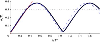
. Figure 6 summarizes the results. The thick black line represents equation (4.9) solved without any approximation. The continuous blue line uses the approximations
 $\unicode[STIX]{x1D70C}=\text{cste}$
and
 $\unicode[STIX]{x1D719}=1-eR/R_{c}$
, while the dashed line uses
 $\unicode[STIX]{x1D719}=\text{cste}=\unicode[STIX]{x1D719}_{eq}$
. As can be seen, these approximations result in negligible errors on the dynamics, with an underestimation of the period of less than
 $1\,\%$
, and approximately
 $4\,\%$
, respectively. The normalization of time in figure 6 with respect to
 $\unicode[STIX]{x1D714}^{\ast }$
predicted by the approximate (4.7) shows that this latter equation provides a good estimate of the dynamics for oscillations of large amplitude (see discussion at the end of § 4.1).
Solution of the modified Rayleigh–Plesset equation for a bubble in an elastic cavity with the physical parameters given in the text. The radius is normalized by the cavity radius, and time is normalized by the period
 $T^{\ast }=1/f^{\ast }=2\unicode[STIX]{x03C0}/\unicode[STIX]{x1D714}^{\ast }$
as predicted by formula (4.7). Black line: exact solution of the equation of motion. Blue lines: solutions obtained with various approximations (continuous: constant density and linearized
 $\unicode[STIX]{x1D719}$
; dashed: constant density and constant
 $\unicode[STIX]{x1D719}$
). Red line: prediction (4.13) of the expansion velocity (arbitrarily going through the origin). The black dotted line represent the equilibrium radius (
 $R=R_{b}$
).

We remark here that the generalized Minnaert formula (4.4) can be obtained by linearization of (4.9) or (4.11) for small excursions
 $\unicode[STIX]{x1D716}$
around
 $R_{eq}$
, leading to the harmonic oscillator equation
 $m\ddot{\unicode[STIX]{x1D716}}+k\unicode[STIX]{x1D716}=0$
of natural angular frequency
 $\unicode[STIX]{x1D714}_{0}=\sqrt{k/m}$
. Also, since we expressed
 $\unicode[STIX]{x1D719}$
as a function of the dimensionless variable
 $x=R/R_{c}$
(see § 3), and since equations (4.9) and (4.11) involve derivatives of
 $\unicode[STIX]{x1D719}$
with respect to
 $R$
, it is useful to relate variations of
 $x$
to variations of
 $R$
. Since both
 $R$
and
 $R_{c}$
vary during bubble motion, this relation is not trivial and follows
 $\text{d}x=\text{d}R/R_{c}-x\,\text{d}R_{c}/R_{c}$
, or
 $$\begin{eqnarray}\frac{\text{d}x}{\text{d}R}=\frac{1}{R_{c}}(1-\unicode[STIX]{x1D705}x^{3}),\end{eqnarray}$$
where we have used (3.3) to eliminate
 $\text{d}R_{c}$
. We finally note from figure 6 that the bubble velocity
 $v_{i}={\dot{R}}$
is approximately constant in many parts of the oscillation when the bubble radius is close to its lowest value. We find that this velocity is well described by the steady-state solution of the unconfined Rayleigh–Plesset equation (neglecting gas pressure and surface tension)
 $$\begin{eqnarray}v_{i}=\sqrt{\frac{2}{3}\frac{-\unicode[STIX]{x0394}P_{0}}{\unicode[STIX]{x1D70C}}}\end{eqnarray}$$
(Brennen Reference Brennen1995), as can be seen from the red line in figure 6.
4.3 Dissipation
For an unconfined bubble, there are three main sources of dissipation during radial oscillations (Leighton Reference Leighton1994): viscous damping due to shear in the liquid, thermal damping due to diffusion of heat in the gas and acoustic radiation. The relative weight of each dissipation source depends on the size of the bubble and thus on the frequency of oscillation, through the Minnaert formula (4.1). Below, we evaluate the impact of the order-of-magnitude increase in oscillation frequency in full confinement (4.6) on the relative importance of these contributions to dissipation. We base our physical discussion on simplified calculations where we consider harmonic oscillations, and where we assume that dissipation coefficients are not modified significantly by confinement; we will thus use expressions obtained for unconfined bubbles.
Damped harmonic oscillations around equilibrium
 $R_{eq}$
follow an equation of the type
 $m\ddot{\unicode[STIX]{x1D716}}+\unicode[STIX]{x1D712}\dot{\unicode[STIX]{x1D716}}+k\unicode[STIX]{x1D716}=0$
with
 $\unicode[STIX]{x1D716}=R-R_{eq}\ll R_{eq}$
and with the dissipation coefficient
 $\unicode[STIX]{x1D712}$
related to the dissipated power through
 ${\mathcal{P}}=\unicode[STIX]{x1D712}\,{\dot{R}}^{2}$
. The system is characterized by its natural pulsation
 $\unicode[STIX]{x1D714}_{0}=\sqrt{k/m}$
and by the quality factor
 $$\begin{eqnarray}Q=\unicode[STIX]{x1D714}_{0}m/\unicode[STIX]{x1D712},\end{eqnarray}$$
which is a dimensionless parameter characterizing damping; a low value of
 $Q$
indicates a large dissipation. We will use the relation
 $\unicode[STIX]{x1D714}_{0}=2\unicode[STIX]{x03C0}{\mathcal{D}}/R_{eq}$
with
 ${\mathcal{D}}$
a constant obtained from (4.4), and an approximate expression for the effective mass
 $m=4\unicode[STIX]{x03C0}\unicode[STIX]{x1D70C}R_{eq}^{3}$
(i.e.
 $\unicode[STIX]{x1D719}\simeq 1$
, see § 3).
Viscous damping is characterized by dissipated power
 ${\mathcal{P}}_{\unicode[STIX]{x1D702}}=16\unicode[STIX]{x03C0}\unicode[STIX]{x1D702}R_{eq}{\dot{R}}^{2}$
and damping coefficient
 $\unicode[STIX]{x1D712}_{\unicode[STIX]{x1D702}}=16\unicode[STIX]{x03C0}\unicode[STIX]{x1D702}R_{eq}$
(Leighton Reference Leighton1994). From (4.14) the corresponding quality factor is
 $$\begin{eqnarray}Q_{\unicode[STIX]{x1D702}}\simeq \frac{\unicode[STIX]{x1D70C}\unicode[STIX]{x1D714}_{0}R_{eq}^{2}}{4\unicode[STIX]{x1D702}}=\frac{\unicode[STIX]{x03C0}\unicode[STIX]{x1D70C}{\mathcal{D}}R_{eq}}{2\unicode[STIX]{x1D702}}.\end{eqnarray}$$
Thermal damping is characterized by the dissipation coefficient
 $\unicode[STIX]{x1D712}_{th}=12\unicode[STIX]{x03C0}R_{eq}k_{p}p_{g,eq}d(\unicode[STIX]{x1D706})/\unicode[STIX]{x1D714}$
where
 $d$
is a dimensionless dissipation function varying between
 $0$
(isothermal or adiabatic) and
 $\simeq 0.11$
(Leighton Reference Leighton1994), and which depends only of the ratio
 $\unicode[STIX]{x1D706}$
of the bubble size
 $R_{eq}$
to the thermal length (
 $\sqrt{D_{g}/(2\unicode[STIX]{x1D714})}$
with
 $D_{g}$
the gas thermal diffusivity). The parameter
 $k_{p}$
is the polytropic exponent, which varies between
 $k_{p}=1$
for purely isothermal and the exponent
 $\unicode[STIX]{x1D6FE}_{a}=C_{p}/C_{v}$
for purely adiabatic transformations (see also § 5.5). Using the above value of
 $\unicode[STIX]{x1D712}_{th}$
, we get from (4.14)
 $$\begin{eqnarray}Q_{th}\simeq \frac{4\unicode[STIX]{x03C0}^{2}}{3d}\frac{\unicode[STIX]{x1D70C}{\mathcal{D}}^{2}}{k_{p}p_{g,eq}}.\end{eqnarray}$$
Acoustic radiation is associated with dissipated power of
 ${\mathcal{P}}=4\unicode[STIX]{x03C0}R_{b}^{2}\unicode[STIX]{x1D70C}C_{\ell }(k_{\ell }R)^{2}{\dot{R}}^{2}$
with
 $k_{\ell }=\unicode[STIX]{x1D714}/C_{\ell }$
the wave vector and
 $C_{\ell }\simeq 1500~\text{m}~\text{s}^{-1}$
the speed of sound in the liquid (Leighton Reference Leighton1994), leading to a damping coefficient
 $\unicode[STIX]{x1D712}_{rad}=4\unicode[STIX]{x03C0}R_{b}^{2}\unicode[STIX]{x1D70C}C_{\ell }(k_{\ell }R_{b})^{2}$
and a quality factor
 $$\begin{eqnarray}Q_{rad}\simeq \frac{C_{\ell }}{\unicode[STIX]{x1D714}_{0}R_{b}}=\frac{C_{\ell }}{2\unicode[STIX]{x03C0}{\mathcal{D}}}.\end{eqnarray}$$
From expressions (4.15)–(4.17), an increase of one order of magnitude of the oscillation speed parameter
 ${\mathcal{D}}$
, as expected for fully confined bubbles, should decrease both viscous and thermal damping, by one and two orders of magnitude respectively. Inversely, acoustic damping is increased by an order of magnitude. Given the fact that in the practical range (bubbles of size
 ${>}1~\unicode[STIX]{x03BC}\text{m}$
), acoustic dissipation is at most
 ${\sim}10$
times weaker than thermal and viscous dissipation (Brennen Reference Brennen1995), we conclude that for fully confined bubbles, acoustic dissipation is on the contrary dominant at more than
 ${\sim}10$
times stronger than viscous dissipation and more than
 ${\sim}10^{2}$
times stronger than thermal dissipation.
We illustrate the previous ideas by using the experimental value
 ${\mathcal{D}}=39~\text{m}~\text{s}^{-1}$
from Vincent et al. (Reference Vincent, Marmottant, Gonzalez-Avila, Ando and Ohl2014a
) and a typical experimental bubble size
 $R_{b}=20~\unicode[STIX]{x03BC}\text{m}$
. From (4.15) we find
 $Q_{\unicode[STIX]{x1D702}}\simeq 6\times 10^{2}$
. From (4.16), using the properties
 $d\leqslant 0.11$
and
 $\unicode[STIX]{x1D705}\leqslant 1.4$
(for air), we evaluate
 $Q_{th}>10^{3}$
for a bubble filled with air at atmospheric pressure. Finally, using (4.17) we estimate
 $Q_{rad}\simeq 6$
, which predicts a very fast attenuation of oscillations, in agreement with experimental results (Vincent et al.
Reference Vincent, Marmottant, Gonzalez-Avila, Ando and Ohl2014a
).
5 Discussion and remarks
Here we compare our results to existing models and experiments, we evaluate some of the hypotheses of our model and we discuss the consequences of the superstability predictions from the bubble statics analysis.
5.1 Comparison with existing bubble dynamics models
As we have discussed in §§ 4.1 and 4.2, our dynamic model reduces to the classical expressions for bubbles in extended liquids (Minnaert, Rayleigh–Plesset) when the size of the bubble is negligible compared to
 $R_{c}$
, more precisely
 $\unicode[STIX]{x1D709}\ll 1$
(4.5). In fact, the case of an unconfined bubble is also obtained when using
 $K_{c}=0$
(no confinement elasticity, resulting in
 $\unicode[STIX]{x1D705}=K_{\ell }/(K_{\ell }+K_{c})=1$
) and replacing the solid density by the density of the liquid, as discussed in the end of § 3. The expression of the static Blake threshold is also recovered when
 $\unicode[STIX]{x1D6FE}\ll 1$
(§ 2.2.2).
Other cases from the literature can be found as limiting cases of our model, for example the case of a bubble in an incompressible liquid within a soft confining solid shell (Fourest et al.
Reference Fourest, Laurens, Deletombe, Dupas and Arrigoni2015) the case of a bubble in a liquid drop surrounded by air (Obreschkow et al.
Reference Obreschkow, Kobel, Dorsaz, de Bosset, Nicollier and Farhat2006). Those both correspond to the limiting case
 $\unicode[STIX]{x1D705}=1$
(confinement much softer than the liquid), with
 $K\neq 0$
and
 $K=0$
, respectively (see appendix B).
Our results also have similarities to dynamic equations derived for bubble oscillations in elastic materials (Alekseev & Rybak Reference Alekseev and Rybak1999; Yang & Church Reference Yang and Church2005; Gaudron, Warnez & Johnsen Reference Gaudron, Warnez and Johnsen2015). Compared to those studies, the case studied here has an extra layer of liquid between the bubble and the elastic materials, which results in additional terms involving the relative elasticities between the liquid and the solid (parameters
 $K$
and
 $\unicode[STIX]{x1D705}$
), and modified liquid kinematics due to confinement (parameter
 $\unicode[STIX]{x1D719}$
). Extending our model to describe this particular case would require setting
 $R_{eq}=R_{c}$
(bubble of the size of the confining cavity, thus no more liquid), a case outside of our small bubble hypothesis. In § 5.3, we suggest ways to modify our model to relax that hypothesis. The studies mentioned above Yang & Church (Reference Yang and Church2005), Gaudron et al. (Reference Gaudron, Warnez and Johnsen2015) have also investigated the effect of viscosity and acoustic radiation on the dynamics, which we have not considered here except in our qualitative discussion of damping sources.
5.2 Comparison with experiments
We now confront our theoretical predictions with experimental results on fully confined cavitation bubbles published recently (Vincent et al.
Reference Vincent, Marmottant, Gonzalez-Avila, Ando and Ohl2014a
). In these experiments, cavitation bubbles spontaneously appeared at a negative pressure
 $\unicode[STIX]{x0394}P_{0}=-20\pm 2$
MPa in water confined in spherical microcavities of radius
 $R_{c}=15{-}200~\unicode[STIX]{x03BC}\text{m}$
etched in a polymer hydrogel material of shear modulus
 $G=0.74\pm 0.08$
GPa (Vincent Reference Vincent2012), see figure 7(a). Statics (equilibrium size) and dynamics (radial oscillations) of the bubble were recorded as a function of confinement size
 $R_{c}$
.
5.2.1 Statics
Bubbles did not contain gases other than the vapour of the liquid so that the trapped gas parameter is
 $\unicode[STIX]{x1D6FC}=0$
(§ 2). In order to estimate the confinement parameter
 $\unicode[STIX]{x1D6FE}$
, we calculate the effective modulus
 $K=(1/K_{\ell }+1/K_{c})$
(2.9) using the confinement elastic modulus
 $K_{c}=4G/3=0.99\pm 0.11$
GPa (see § 2.1) and the liquid water modulus (
 $K_{\ell }=2.195\pm 0.016$
GPa in the range
 $20{-}25\,^{\circ }\text{C}$
, see Kell (Reference Kell1975)). We obtain
 $K=0.68\pm 0.07$
GPa and the corresponding dimensionless value
 $\unicode[STIX]{x1D705}=K_{\ell }/(K_{\ell }+K_{c})=0.69\pm 0.03$
. Using
 $\unicode[STIX]{x1D70E}=0.072~\text{N}~\text{m}^{-1}$
for water and considering that the microcavity size is
 $R_{c}>15~\unicode[STIX]{x03BC}\text{m}$
, we thus estimate
 $\unicode[STIX]{x1D6FE}<10^{-8}$
from (2.16). These values of
 $\unicode[STIX]{x1D6FC}$
and
 $\unicode[STIX]{x1D6FE}$
place the experiments in regime
 $\unicode[STIX]{x2461}$
of the phase diagram where the macroscopic bubble of radius
 $R_{eq}=R_{b}$
is the most stable solution, and far away from any of the transition lines, in particular the transition lines to superstability. We discuss in § 5.6 the possibility of realizing experiments probing the superstability transition. The low value of
 $\unicode[STIX]{x1D6FE}$
also allows us to use formula (2.19) which predicts a linear relationship between the bubble equilibrium size
 $R_{eq}$
and the microcavity size
 $R_{c}$
, with a coefficient
 $$\begin{eqnarray}x_{eq}=R_{eq}/R_{c}=(-\unicode[STIX]{x0394}P_{0}/K)^{1/3}.\end{eqnarray}$$
With the parameter values specified above, we predict
 $x_{eq}=0.31\pm 0.02$
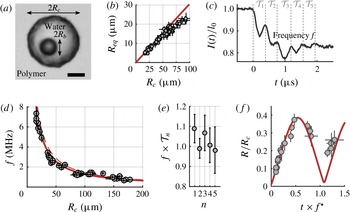
which gives good agreement with the experimental data (thick red line in figure 7
b). Departures from the prediction can be observed for big radii; they might be due to non-sphericity of the larger microcavities or to optical deformations of the bubble as seen through the liquid/polymer interface (Vincent Reference Vincent2012).
5.2.2 Dynamics
Although the value of the static confinement parameter
 $\unicode[STIX]{x1D6FE}$
is very low, the criterion for fully confined dynamics is governed by the dynamic confinement parameter
 $\unicode[STIX]{x1D709}=|K/K_{b}|(R_{b}/R_{c})^{3}$
(see § 4.1), estimated to be
 $\unicode[STIX]{x1D709}>(42/3)^{3}\simeq 3\times 10^{3}$
(Vincent et al.
Reference Vincent, Marmottant, Gonzalez-Avila, Ando and Ohl2014a
). Since
 $\unicode[STIX]{x1D709}\gg 1$
, the compressibility of the liquid and the elasticity of the confinement dominate the dynamics, which allows us to use formula (4.6) for the natural oscillation frequency, which can be rewritten
 $f_{0}=(1/2\unicode[STIX]{x03C0}R_{c})\sqrt{3K/\unicode[STIX]{x1D70C}\unicode[STIX]{x1D719}_{eq}}(-\unicode[STIX]{x0394}P_{0}/K)^{1/6}$
using equation (5.1). As can be seen in figure 7(d) (dashed line), this prediction (numerically
 $f_{0}\times R_{c}=143\pm 8~\text{m}~\text{s}^{-1}$
) matches experimental results very well using a kinematic correction factor
 $\unicode[STIX]{x1D719}_{eq}=0.79$
(see § 3.3), but slightly overestimates the frequency. As explained in § 4.1, this is likely due to anharmonic effects for large oscillations, and the approximate (4.7) (numerically
 $f^{\ast }\times R_{c}=128\pm 7~\text{m}~\text{s}^{-1}$
) works better in that case (continuous line in figure 7
d).
Comparison between available experimental data, mostly from Vincent et al. (Reference Vincent, Marmottant, Gonzalez-Avila, Ando and Ohl2014a
) (black or grey data), and the theory developed in the present paper (thick red lines). (a) Typical microphotograph of the experimental system (scale bar:
 $20~\unicode[STIX]{x03BC}\text{m}$
), showing the bubble after spontaneous cavitation. (b) Equilibrium bubble radius as a function of microcavity radius (theory: equation (5.1)). (c) Extinction signal associated with a cavitation event (cavitation at
 $t=0$
),
 ${\mathcal{T}}_{n}$
represents the period of the
 $n\text{th}$
oscillation. (d) Oscillation frequency as a function of microcavity radius compared to equations (4.6) (dashed line) and (4.7) (continuous line). (e) Ratio of
 ${\mathcal{T}}_{n}$
to the average period
 $1/f$
, including all experiments (Vincent Reference Vincent2012). (f) Radial bubble dynamics extracted from laser strobe photography experiments (Vincent et al.
Reference Vincent, Marmottant, Gonzalez-Avila, Ando and Ohl2014a
). Theory: equation (4.9) solved with initial conditions
 $R/R_{c}=0.02$
and
 ${\dot{R}}=0$
.

Anharmonic effects (appendix A) probably explain the decrease in the oscillation period observed experimentally (figure 7
e) and are naturally included in the full equation of motion (modified Rayleigh–Plesset equation (4.9)). The latter shows excellent agreement with direct measurements of the
 $R(t)$
bubble dynamics (figure 7
f).The fact that the experimental datapoints sit above the theoretical curve before and after
 $t\times f^{\ast }\simeq 1$
is probably due to the fact that dissipation is not taken into account in (4.9).
Finally, the typical number of oscillations (
 $5{-}6$
) from the experimental recordings (figure 7
c) is in excellent agreement with the prediction of a quality factor
 $Q\simeq 6$
for acoustic dissipation (see § 4.3), which supports our conclusion that acoustic damping is dominant over viscous and thermal damping for fully confined bubbles.
We emphasize here the excellent agreement between the experimental data and the model without adjustable parameters. Since cavitation bubbles in experiments are unlikely to be centred in the cavity, this good agreement suggests that corrections due to off-centred bubbles, as discussed in § 5.3 below, are small.
5.3 Size, shape and position of the bubble and cavity
We have used linear expansions of the equation of state for
 $\unicode[STIX]{x0394}P_{0}$
, assuming that the relative volume changes of the liquid and of the cavity were small. These changes are of the order of
 $V_{b}/V_{c}$
, leading to a condition of validity
 $(R_{b}/R_{c})^{3}\ll 1$
. As mentioned in § 1, this condition is not very restrictive. For example, in the cavitation experiments reported in § 5.2,
 $(R_{b}/R_{c})^{3}=x_{eq}^{3}\simeq 0.03$
. We note that larger bubble sizes can in fact be accommodated in our model by taking as a reference state not the value
 $R=0$
but a non-zero value for which the bubble has a volume
 $V_{ref}$
. In this case, equations (2.9), (3.1) and (3.2) have to be changed to
 $K=K_{\ell }/([1-x_{ref}^{3}+K_{\ell }/K_{c}])$
,
 $V_{c}=V_{0}+\unicode[STIX]{x1D705}(V-V_{ref})$
and
 $\unicode[STIX]{x1D70C}=\unicode[STIX]{x1D70C}_{ref}[1-\unicode[STIX]{x1D705}(x^{3}-x_{ref}^{3})-x_{ref}^{3}]/[1-x^{3}]$
, respectively, where we have defined
 $x_{ref}^{3}=V_{ref}/V_{0}$
and
 $\unicode[STIX]{x1D705}=K/K_{c}$
.
The hypothesis of a bubble at the centre of the confining cavity is not necessary for the static calculation of the potential
 $F(R)$
, but matters for the kinematic calculation of the effective mass. Indeed an oscillating bubble in an off-centred position would generate a non-radial flow field, resulting in a modified effective mass compared to our radial calculation. Although the calculation of this effect is quite complicated and outside of the scope of this article, the good agreement between our model and experimental results suggest that this effect might be weak (see § 5.2). In fact, for an unconfined bubble in the vicinity of a wall, the kinetic energy (and thus the effective mass) is decreased by approximately
 $20\,\%$
at maximum (Strasberg Reference Strasberg1953).
We have assumed that both bubble and cavity were spherical. In fact, the two most important contributions to the free energy in fully confined situations (liquid compressibility and solid deformability) only depend on volume (
 $V$
) change, so these hypotheses can be relaxed by defining the radii (
 $R$
) of both bubble and cavity as
 $R=[3V/(4\unicode[STIX]{x03C0})]^{1/3}$
. In the statics and potential energy calculations, such a substitution should be valid provided that the surface tension term is modified as well, and the value of
 $K_{c}$
adapted to the specific geometry of interest too. For the dynamics, a non-spherical bubble or cavity create non-radial flow fields and the substitution is thus less straightforward.
5.4 Quasi-static hypothesis
To calculate the kinematics and dynamics (§§ 3 and 4), we have assumed that the bubble was evolving quasi-statically, and in particular that the density was uniform in the liquid during the oscillation. We have verified that for small amplitude oscillations, the predictions of our model were in excellent agreement with an acoustic calculation taking into account spatial pressure and density variations around a finite-size bubble in rigid confinement (appendix C). For larger oscillations, we expect that our modified Rayleigh–Plesset equation still describes the dynamics well, as it includes all the essential physics (modified kinematics, temporal density variations, nonlinearity of the potential, compressibility of liquid and solid phases etc.), but would need to include second-order corrections to be exact. The good agreement between our model and the available experimental data (§ 5.2) suggests that these corrections are small, but experimental errors make it difficult to quantify them precisely. This opens perspectives for future experimental and simulation work to clarify these questions.
It may seem surprising that our mean-field approach compares so well with acoustic calculations. Below, we provide suggestions that might explain this success. First, as discussed in § 4.2, due to the low compressibility of the liquid, density variations are small. As a result, a spatially varying density should have only weak effects on the velocity profile calculated for the kinematics (§ 3), which is mainly constrained by the boundary conditions at the bubble surface and at the cavity surface (see figure 5). Second, it is also reasonable to think that the elastic response of the liquid and of the solid as they are compressed and stretched during bubble oscillation (i.e. the main contribution to the stiffness for fully confined bubbles) is mainly sensitive to global deformations and not to details of the density distribution associated with these global deformations. Last, we expect gradients of pressure and density during the oscillation to be located in the vicinity of the bubble surface so that most of the liquid volume achieves values of these parameters close to the average ones. The results of appendix C also suggest that the acoustic wavelength, which describes the typical distance across which the fields are expected to vary, is large compared to the cavity size.
5.5 Thermal effects
To allow for simple comparison with established formula of bubble dynamics and nucleation theories, we have assumed that the system behaved isothermally. While this hypothesis may seem questionable in regard to the very fast dynamics associated with confined bubbles, we show below that this choice has little impact on the predicted dynamics, and we suggest alternative expressions for adiabatic behaviour.
For fully confined bubbles, the key mechanical ingredients setting the dynamics are the bulk modulus
 $K_{\ell }$
of the liquid and the confinement modulus
 $K_{c}$
which depends on the solid shear modulus
 $G$
. These moduli depend weakly on the thermodynamic path of the transformations. For example, for water in the temperature range
 $20{-}30\,^{\circ }\text{C}$
,
 $K_{\ell }$
(isothermal) differs from
 $K_{\ell ,S}$
(adiabatic) by less than
 $1.5\,\%$
(Del Grosso & Mader Reference Del Grosso and Mader1972; Kell Reference Kell1975). In fact, due to the large heat capacity of the liquid, it is reasonable to assume an isothermal evolution outside of the bubble. However, in the case where the bubble contained trapped gas, this gas can undergo isothermal to adiabatic transformations depending on the oscillation frequency and the size of the bubble (Brennen Reference Brennen1995). This is usually taken into account by considering a polytropic exponent
 $k_{p}$
(varying between
 $k_{p}=1$
for purely isothermal and the exponent
 $\unicode[STIX]{x1D6FE}_{a}=C_{p}/C_{v}$
for purely adiabatic transformations). The gas pressure follows
 $p_{g}(R)=p_{g,eq}(R_{b}/R)^{3k_{p}}$
resulting in a contribution
 $k_{p}\times p_{g,eq}$
instead of
 $p_{g,eq}$
in the oscillation stiffness. We expect that using such a substitution in our expression of
 $K_{b}$
(4.2), and using the polytropic variation of
 $p_{g}$
in the Rayleigh–Plesset equations (4.9), (4.11) should allow describing dynamics in non-isothermal situations.
5.6 Liquid superstability
The results from § 2.2.1 predict that no nucleation is possible in a liquid at negative pressure if the liquid is confined to a sufficiently small volume, because compressing the liquid (and/or solid) to grow the bubble is unfavourable. Equivalently, from (2.16), for a given confinement radius
 $R_{c}$
, the liquid is stable if the tension is low enough, i.e. the negative pressure in the liquid
 $\unicode[STIX]{x0394}P_{0}$
is above a value
 $$\begin{eqnarray}(\unicode[STIX]{x0394}P_{0})_{t}=-\left(\frac{8\unicode[STIX]{x1D70E}^{3}K}{R_{c}^{3}\unicode[STIX]{x1D6FE}_{t}}\right)^{1/4}.\end{eqnarray}$$
Using the properties of water
 $\unicode[STIX]{x1D70E}=0.072~\text{N}~\text{m}^{-1}$
and
 $K=2.2$
GPa (assuming an infinitely stiff confinement), one obtains the numerical values of figure 8(a) (continuous line). Also plotted as a dashed line is the value
 $(\unicode[STIX]{x0394}P_{0})_{s}$
obtained by replacing
 $\unicode[STIX]{x1D6FE}_{t}$
by
 $\unicode[STIX]{x1D6FE}_{s}$
in (5.2). This other transition line corresponds to the disappearance of the bubble solution and thus corresponds to a spinodal beyond which the negative pressure liquid is not only stable, but the only state accessible in the system. As seen on figure 8(a), the two transitions are close. This superstabilization effect was noticed by MacDowell, Shen & Errington (Reference Macdowell, Shen and Errington2006) and later by Vincent (Reference Vincent2012), Wilhelmsen et al. (Reference Wilhelmsen, Bedeaux, Kjelstrup and Reguera2014) for nucleation in small systems with fixed volume and number of particles. The present model considers a more general case with elastic confinement and trapped gas, as well as dynamic situations.
Due to superstabilization, nucleation is suppressed not only when the confinement size is less than the critical radius
 $R^{\ast }$
, as often argued in the literature (Or & Tuller Reference Or and Tuller2002; Tas et al.
Reference Tas, Mela, Kramer, Berenschot and van den Berg2003), but even at much larger dimensions in fully confined situations. Indeed, combining (2.21), (2.12) and (5.4) yields the ratio
 $$\begin{eqnarray}\left(\frac{R_{c}}{R^{\ast }}\right)_{t}=2\left(\frac{2K}{-\unicode[STIX]{x0394}P_{0}}\right)^{1/3}\end{eqnarray}$$
below which a liquid at negative pressure
 $\unicode[STIX]{x0394}P_{0}$
is absolutely stable. With typical negative pressures in the MPa range and liquid/solid bulk moduli in the GPa range, this ratio is typically larger than
 $10$
.
(a) Liquid superstability with respect to nucleation in confinement. The continuous line is the transition line above which the liquid is absolutely stable (5.2), and the dashed line is the spinodal line above which the homogeneous liquid is the only possible equilibrium solution (equation (5.2) with
 $\unicode[STIX]{x1D6FE}_{s}$
instead of
 $\unicode[STIX]{x1D6FE}_{t}$
). (b) Spontaneous collapse of pre-existing bubbles in confinement. Continuous and dashed lines have the same signification as in (a) and correspond to (5.4) and (5.5), respectively.

The superstabilization effect should be still present in situations where the liquid is not strictly trapped in the cavity but where the time scales of liquid flow in and out of the cavity are long compared to bubble dynamics time scales. This criterion is verified in experimental systems consisting of microcavities surrounded by polymer hydrogels (Wheeler & Stroock Reference Wheeler and Stroock2008, Reference Wheeler and Stroock2009; Vincent et al.
Reference Vincent, Marmottant, Quinto-Su and Ohl2012, Reference Vincent, Marmottant, Gonzalez-Avila, Ando and Ohl2014a
) or porous silicon (Vincent et al.
Reference Vincent, Sessoms, Huber, Guioth and Stroock2014b
). These controlled platforms might thus provide ways to investigate the superstabilization effect experimentally. In such systems, cavitation typically spontaneously occurs at
 $-20$
MPa (Wheeler & Stroock Reference Wheeler and Stroock2008; Vincent et al.
Reference Vincent, Sessoms, Huber, Guioth and Stroock2014b
). According to figure 8(a), a full confinement of dimensions
 $R_{c}\simeq 100$
nm and below would suppress cavitation at that value of negative pressure. This dimension is clearly associated with experimental challenges for the fabrication and observation of submicrometre cavities, but could open perspectives to study the behaviour of liquids in large tensions usually not accessible due to spontaneous cavitation.
5.7 Spontaneous bubble collapse
The results discussed above also predict that, in full confinement, no bubble can exist below a certain size: there are only solutions for the existence of a bubble above
 $R_{s}=4R^{\ast }/3$
and this solution is only metastable between
 $R_{s}$
and
 $R_{t}=2R^{\ast }$
(figure 4(a) and (2.21)). We eliminate
 $R^{\ast }$
then
 $\unicode[STIX]{x0394}P_{0}$
from these expressions using (2.12) and (2.17), respectively. Solving for
 $R_{b}=R_{t}$
using (2.21), we obtain
 $$\begin{eqnarray}\frac{R_{t}}{R_{c}}=\left(\frac{2\unicode[STIX]{x1D70E}}{R_{c}K}\right)^{1/4},\end{eqnarray}$$
where we have expressed the result in terms of ratio to the size of the confinement. Similarly, using (2.23) we obtain
 $$\begin{eqnarray}\frac{R_{s}}{R_{c}}=\left(\frac{2\unicode[STIX]{x1D70E}}{3R_{c}K}\right)^{1/4},\end{eqnarray}$$
where it can be noticed that
 $R_{t}=3^{1/4}R_{s}\simeq 1.32\,R_{s}$
. Equation (5.5) establishes the smallest bubble that can exist in a container of size
 $R_{c}$
. As can be seen in figure 8(b), where the transition line
 $R_{t}$
is plotted as a full line and the spinodal line
 $R_{s}$
is plotted as a dashed line using the values of
 $\unicode[STIX]{x1D70E}$
and
 $K$
for water (see above), containers in the sub-
 $\unicode[STIX]{x03BC}\text{m}$
range do not allow bubbles that are smaller than typically
 $10{-}20\,\%$
of their own size.
This effect can be important in the context of geological fluid inclusions where the static evolution of bubbles is used to determine the properties of the naturally enclosed liquid (Marti et al.
Reference Marti, Krüger, Fleitmann, Frenz and Rička2012). In such studies, the sample is heated up until the existing bubble disappears from the thermal expansion of the liquid. The effect described here leads to a premature spontaneous collapse of the bubble when it reaches
 $R_{s}$
and may thus induce artefacts in the estimate of the homogenization temperature (Marti et al.
Reference Marti, Krüger, Fleitmann, Frenz and Rička2012). One may also wonder if the spontaneous collapse of bubbles could also play a role in the debated phenomenon of spontaneous refilling of embolized tree vessels (Holbrook & Zwieniecki Reference Holbrook and Zwieniecki1999; Stroock et al.
Reference Stroock, Pagay, Zwieniecki and Michele Holbrook2014).
6 Conclusion
Fully confined bubbles, i.e. bubbles in a liquid in a solid (extended or in the form of a shell), are unique because any change in their size must be accommodated by compression or stretching of the liquid and/or deformation of the solid. As we showed in this article, this simple statement has many implications, both for the statics and the dynamics of those bubbles.
In static situations, confinement only modifies Blake’s threshold (gas parameter
 $\unicode[STIX]{x1D6FC}$
) in a weak manner, but is responsible for the superstability of confined liquids which may become absolutely stable even at negative pressure, and for the spontaneous collapse of confined bubbles towards a homogeneous, negative pressure liquid. These phenomena are governed by the static confinement parameter
 $\unicode[STIX]{x1D6FE}$
and result from the interplay of surface tension and the deformability of both the liquid and the solid.
In dynamic situations, confinement has several implications. First, it decreases the system inertia by imposing a faster radial decrease of the liquid velocity, controlled by the dimensionless elastic parameter
 $\unicode[STIX]{x1D705}$
. Infinitely stiff confinements (
 $\unicode[STIX]{x1D705}=0$
) provide the strongest correction compared to a bubble in an extended liquid whereas for soft confinements (
 $\unicode[STIX]{x1D705}\simeq 1$
), this decrease can be compensated by the inertia of the moving solid. Second, confinement forces the involvement of both liquid compressibility and solid deformability in the stiffness of the system, in addition to the contributions of inner gas and surface tension. We showed that the interplay between these elements resulted in a picture with some stiffnesses in series and others in parallel, with relative contributions characterized by the dynamic confinement parameter
 $\unicode[STIX]{x1D709}$
. In particular, for
 $\unicode[STIX]{x1D709}\gg 1$
, the liquid and solid deformabilities dominate the stiffness of the system, resulting in order-of-magnitude increase of the oscillation frequency compared to unconfined bubbles. An interesting consequence of this fast dynamics is the largely increased contribution of acoustic damping compared to viscous and thermal dissipations.
We have shown that the predictions of our model were in excellent agreement with recent experiments (with parameters
 $\unicode[STIX]{x1D6FC}=0$
,
 $\unicode[STIX]{x1D6FE}\ll 1$
,
 $\unicode[STIX]{x1D705}=0.7$
and
 $\unicode[STIX]{x1D709}\gg 1$
), and we have also discussed how the generality of our dynamic equations allow us to describe a variety of situations including bubbles in drops, or bubbles in liquids confined in soft or rigid shells, by using appropriate values for the dimensionless parameters.
Appendix A. Anharmonic corrections
We evaluate the effect of the anharmonicity of the potential for
 $\unicode[STIX]{x1D709}\gg 1$
. In this regime, from (2.10), the potential takes the simple form
 $$\begin{eqnarray}F(R)=F_{b}\left(\frac{R}{R_{b}}\right)^{3}\left[\left(\frac{R}{R_{b}}\right)^{3}-2\right]=F_{b}\left(\left[\left(\frac{R_{b}}{R_{c}}\right)^{3}-1\right]^{2}-1\right),\end{eqnarray}$$
with
 $F_{b}=(1/2)V_{b}(-\unicode[STIX]{x0394}P_{0})=(1/2)(V_{c}/K)\unicode[STIX]{x0394}P_{0}^{2}$
where
 $V_{b}$
is the equilibrium bubble volume and
 $V_{c}$
is the cavity volume. Comparing equation (A 1) to its quadratic approximation (see figure 9), it is clear that considerable deviations must occur for large oscillations compared to the harmonic behaviour. The effective mass itself is also not a constant as a function of bubble radius and typically grows as
 $R^{3}$
(e.g. (3.14)). Both effects are antagonistic: while the stiffness increases above
 $R_{b}$
, increasing the oscillation frequency, the effective mass also increases, which decreases the oscillation frequency.
We first neglect the mass contributions (
 $\unicode[STIX]{x1D719}=1$
) and we consider an oscillation of amplitude
 $\unicode[STIX]{x0394}R$
between a radius
 $R_{min}$
and a radius
 $R_{max}$
while the free energies at these radii are
 $F(R_{min})=F(R_{max})=-F_{b}+\unicode[STIX]{x1D6FF}F$
, where
 $F_{b}$
is the potential well depth defined above and where
 $\unicode[STIX]{x1D6FF}F$
represents the energy above equilibrium (see figure 9
a). From the conservation of the total energy
 $E_{k}+F(R)$
,
 $$\begin{eqnarray}\frac{1}{2}4\unicode[STIX]{x03C0}\unicode[STIX]{x1D70C}R^{3}\left(\frac{\text{d}R}{\text{d}t}\right)^{2}+F(R)=-F_{b}+\unicode[STIX]{x1D6FF}F.\end{eqnarray}$$
Extracting
 $\text{d}t$
from this equation allows us to calculate the value of half a period by integration between
 $R_{min}$
and
 $R_{max}$
. We define the parameters
 $\unicode[STIX]{x1D703}=\sqrt{\unicode[STIX]{x1D6FF}F/F_{b}}$
, which quantifies the energy of the oscillations relative to the potential well depth, and
 $u=[(R/R_{b})^{3}-1]/\unicode[STIX]{x1D703}$
so that
 $u$
varies monotonically between
 $-1$
and
 $1$
when
 $R$
varies between
 $R_{min}$
and
 $R_{max}$
, and
 $[F(R)+F_{b}]/\unicode[STIX]{x1D6FF}F=u^{2}$
from (A 1). We finally obtain the total period
 $$\begin{eqnarray}{\mathcal{T}}={\mathcal{T}}_{0}\int _{-1}^{1}\frac{\text{d}u}{\unicode[STIX]{x03C0}\sqrt{1-u^{2}}}(1+\unicode[STIX]{x1D703}u)^{-1/6},\end{eqnarray}$$
where
 ${\mathcal{T}}_{0}=1/f_{0}$
is the small-amplitude period (
 ${\mathcal{T}}_{0}=1/f_{0}$
from (4.6)). Using
 $F(R_{min,max})=-F_{b}+\unicode[STIX]{x1D6FF}F$
we also get
 $R_{min,max}=R_{b}(1\mp \unicode[STIX]{x1D703})^{1/3}$
so that the amplitude of the oscillations is
 $$\begin{eqnarray}\unicode[STIX]{x0394}R=R_{b}\left[(1+\unicode[STIX]{x1D703})^{1/3}-(1-\unicode[STIX]{x1D703})^{1/3}\right],\end{eqnarray}$$
which we develop to the lowest order into
 $\unicode[STIX]{x0394}R\simeq 2\unicode[STIX]{x1D703}R_{b}/3$
. Using the same procedure on (A 3) leads to
 ${\mathcal{T}}\simeq {\mathcal{T}}_{0}(1+(7/144)\unicode[STIX]{x1D703}^{2})$
. Combining these two expressions leads to a generalized Borda formula (in analogy with pendulum mechanics)
 $$\begin{eqnarray}\unicode[STIX]{x1D701}=\frac{{\mathcal{T}}}{{\mathcal{T}}_{0}}\simeq 1+\frac{7}{64}\left(\frac{\unicode[STIX]{x0394}R}{R_{b}}\right)^{2},\end{eqnarray}$$
which represents the nonlinear correction at the lowest order. This prediction is plotted as a thin green line of figure 9 where we also plotted the exact solution by numerical integration of (A 3), see the thick green line. We note that the maximum oscillation amplitude is obtained for
 $\unicode[STIX]{x1D6FF}F=F_{b}$
or
 $\unicode[STIX]{x1D703}=1$
. From (A 4), this occurs when
 $\unicode[STIX]{x0394}R/R_{b}=2^{1/3}\simeq 1.26$
.
Anharmonic effects. (a) Thick black line: shape of the potential
 $F(R)$
from (A 1), dashed line: harmonic approximation (see § 4.1). The blue arrow represents the oscillation for an energy
 $\unicode[STIX]{x1D6FF}F$
, corresponding to an oscillation amplitude
 $\unicode[STIX]{x0394}R$
. (b) Oscillation period as a function of
 $\unicode[STIX]{x0394}R$
. Green squares correspond to simulations with the simplified case
 $m=m_{\infty }$
, while red circles corresponds simulations in the rigid, confined case
 $m=\unicode[STIX]{x1D719}\times m_{\infty }$
(fitted with
 ${\mathcal{T}}/{\mathcal{T}}_{0}\simeq 1+(\unicode[STIX]{x0394}R/R_{b})^{2}/6$
, thin red line). Thick green line: theoretical period from (A 3), thin green line: Borda formula with
 $m=m_{\infty }$
(A 5).

We have assumed up to now that the effective mass was
 $m_{\infty }=4\unicode[STIX]{x03C0}\unicode[STIX]{x1D70C}R^{3}$
whereas confinement induces a correcting factor
 $\unicode[STIX]{x1D719}$
that depends on
 $R$
and thus introduces additional nonlinearities. In order to evaluate the importance of this effect, we use results of simulations of the complete equation of motion using
 $m(R)=\unicode[STIX]{x1D719}m_{\infty }$
in the case of a rigid confinement (
 $K=K_{\ell }$
), for which the effective mass deviates most from the unconfined case (see § 3). Results are displayed as red data in figure 9, showing that the effective mass corrections introduce further deviations from the harmonic behaviour. In general, a system where confinement is not fully rigid has an effective mass comprised between the effective mass of a bubble in an infinite liquid and that of a bubble in a rigid confinement. We thus expect that the green and red data bound the possible nonlinear corrections to the oscillation period.
Appendix B. Special cases of the confined Rayleigh–Plesset equation
Here we show that our modified Rayleigh–Plesset equation for fully confined bubbles admits established results as limiting cases, namely softly confined cases where the confinement cavity is much more compliant than the liquid, so that the latter can be considered as incompressible. This is the case in the calculations of Fourest et al. (Reference Fourest, Laurens, Deletombe, Dupas and Arrigoni2015) who considered a bubble in a liquid confined in a soft shell, assuming an incompressible liquid, and neglecting the inertia of the shell during bubble dynamics. An extreme case is also the case of a bubble in a drop, where the ‘confinement’ is made by air. This situation was considered by Obreschkow et al. (Reference Obreschkow, Kobel, Dorsaz, de Bosset, Nicollier and Farhat2006). As discussed in § 3 here, the soft confinement hypothesis entails
 $\unicode[STIX]{x1D705}=1$
, resulting in
 $\unicode[STIX]{x1D70C}=\unicode[STIX]{x1D70C}_{0}$
(constant liquid density) and
 $\unicode[STIX]{x1D719}=1-x$
from (3.2) and (3.15), when solid inertia is absent or neglected. As a result,
 $\text{d}\unicode[STIX]{x1D719}/\text{d}R=-\text{d}x/\text{d}R=-1/R_{c}(1-x^{3})$
from (4.12), or
 $\text{d}\ln \unicode[STIX]{x1D719}/\text{d}\ln R=(R/\unicode[STIX]{x1D719})\,\text{d}\unicode[STIX]{x1D719}/\text{d}R=-x(1-x^{3})/(1-x)$
. Thus, from (4.9)
 $$\begin{eqnarray}R\ddot{R}+\left(\frac{3}{2}-\frac{1}{2}\frac{x}{1-x}(1-x^{3})\right){\dot{R}}^{2}=-\frac{\unicode[STIX]{x0394}P(R)}{\unicode[STIX]{x1D70C}(1-x)},\end{eqnarray}$$
where we have noted
 $\unicode[STIX]{x0394}P(R)=\unicode[STIX]{x0394}P_{0}+K(R/R_{c})^{3}$
the liquid pressure as a function of bubble size (neglecting surface tension and trapped gas). Multiplying by
 $1-x$
and rearranging the terms yields
 $$\begin{eqnarray}R\ddot{R}+\frac{3}{2}{\dot{R}}^{2}-xR\ddot{R}-2x{\dot{R}}^{2}+\frac{1}{2}x^{4}{\dot{R}}^{2}=-\frac{\unicode[STIX]{x0394}P(R)}{\unicode[STIX]{x1D70C}},\end{eqnarray}$$
which is exactly the equations derived by Obreschkow et al. (Reference Obreschkow, Kobel, Dorsaz, de Bosset, Nicollier and Farhat2006), Fourest et al. (Reference Fourest, Laurens, Deletombe, Dupas and Arrigoni2015). In the case of an air confinement such as in Obreschkow et al. (Reference Obreschkow, Kobel, Dorsaz, de Bosset, Nicollier and Farhat2006), there is no elastic component in
 $\unicode[STIX]{x0394}P(R)$
(
 $K=0$
,
 $\unicode[STIX]{x0394}P$
constant), while a non-zero value of
 $K$
has to be used in the case of an elastic shell confinement as in Fourest et al. (Reference Fourest, Laurens, Deletombe, Dupas and Arrigoni2015). The value of
 $K$
for an elastic shell is discussed in § 2.1 here.
Appendix C. Acoustic calculation for small oscillations
Here we search, for a bubble of size
 $R_{b}$
confined in a spherical cavity of radius
 $R_{c}$
, what is the condition for the existence of a bubble oscillation at pulsation
 $\unicode[STIX]{x1D714}=2\unicode[STIX]{x03C0}f$
, linked to the establishment of acoustic waves in the cavity. We assume that the cavity is perfectly rigid (
 $K=K_{\ell }$
) and that the oscillations are of small amplitude so that fluctuations of pressure around equilibrium can be described by the acoustic wave equation
 $C_{\ell }^{2}\unicode[STIX]{x1D6FB}^{2}p=\unicode[STIX]{x2202}^{2}p/\unicode[STIX]{x2202}t^{2}$
where
 $C_{\ell }=\sqrt{K_{\ell }/\unicode[STIX]{x1D70C}}$
is the velocity of sound in the liquid. In a radial symmetry, the solutions take the form (Landau & Lifshitz Reference Landau and Lifshitz1987)
 $$\begin{eqnarray}p(r,t)=\left(\frac{A}{r}\text{e}^{\text{i}kr}+\frac{B}{r}\text{e}^{-\text{i}kr}\right)\text{e}^{-\text{i}\unicode[STIX]{x1D714}t},\end{eqnarray}$$
where
 $k_{\ell }=2\unicode[STIX]{x03C0}/\unicode[STIX]{x1D706}=\unicode[STIX]{x1D714}/C_{\ell }$
is the wave vector in the liquid, and where
 $A$
and
 $B$
are complex constants. The velocity
 $\boldsymbol{v}=v(r)\boldsymbol{u}_{r}$
is deduced from the Euler equation
 $\unicode[STIX]{x1D70C}\unicode[STIX]{x2202}\boldsymbol{v}/\unicode[STIX]{x2202}t=-\unicode[STIX]{x1D735}p$
, which gives
 $-\text{i}\unicode[STIX]{x1D714}\unicode[STIX]{x1D70C}v=-\unicode[STIX]{x2202}p/\unicode[STIX]{x2202}r$
using the notations defined above, and
 $$\begin{eqnarray}v(r,t)=\frac{\text{i}}{\unicode[STIX]{x1D70C}\unicode[STIX]{x1D714}}\left(A\left[\frac{1}{r^{2}}-\frac{\text{i}k_{\ell }}{r}\right]\text{e}^{\text{i}k_{\ell }r}+B\left[\frac{1}{r^{2}}+\frac{\text{i}k_{\ell }}{r}\right]\text{e}^{-\text{i}k_{\ell }r}\right)\text{e}^{-\text{i}\unicode[STIX]{x1D714}t}.\end{eqnarray}$$
The boundary conditions are
 $p(R)=0$
at the bubble wall and
 $v(R_{c})=0$
on the solid wall. This allows us to determine
 $A=-B\text{e}^{-2\text{i}k_{\ell }R}$
from equations (C 1) and (C 2), and to establish the necessary condition for the existence of stationary waves in the liquid as
 $\tan (k_{\ell }[R_{c}-R_{b}])=k_{\ell }R_{c}$
or
 $$\begin{eqnarray}\tan \left(\frac{2\unicode[STIX]{x03C0}{\mathcal{D}}}{C_{\ell }x}\left[1-x\right]\right)=\frac{2\unicode[STIX]{x03C0}{\mathcal{D}}}{C_{\ell }x},\end{eqnarray}$$
where we have used the notations
 $x=R_{b}/R_{c}$
and
 ${\mathcal{D}}=f\times R_{b}$
. This equation has an infinite number of solutions, corresponding to different modes of oscillation. We consider only the lowest non-zero frequency mode corresponding to the natural frequency and compare the solution for
 ${\mathcal{D}}(x)$
to the prediction of our quasi-static (QS) model:
 $$\begin{eqnarray}{\mathcal{D}}=\frac{C_{\ell }}{2\unicode[STIX]{x03C0}}\left(\frac{3}{\unicode[STIX]{x1D719}}\right)^{1/2}x^{3/2}\end{eqnarray}$$
using (4.4) with
 $\unicode[STIX]{x1D719}$
the kinetic correction factor as defined in § 3, with
 $K=K_{\ell }=\unicode[STIX]{x1D70C}C_{\ell }^{2}$
, and neglecting surface tension or trapped gas (
 $K_{b}=0$
).
As can be seen in figure 10(a), the agreement between the acoustic and the QS approaches is excellent, with a difference of less than
 $1\,\%$
for
 $x=0{-}0.44$
. The predictions start diverging more visibly for higher values of
 $x$
, a regime outside the domain of validity of our hypothesis of small bubbles (see §§ 1 and 5.3).
(a) Comparison between the acoustic predictions and our quasi-static model for
 ${\mathcal{D}}=\,f\times R_{b}$
as a function of the dimensionless equilibrium radius
 $x=R_{b}/R_{c}$
. Inset: ratio between the acoustic and quasi-static models. (b) Spatial variations of the pressure (top), and the velocity (bottom), calculated with the acoustic (black dots) and quasi-static (red line) models.

Injecting
 $A$
and
 $B$
in (C 1) and (C 2), we also find
 $$\begin{eqnarray}\displaystyle & \displaystyle p(r,t)=\langle p(t)\rangle \frac{1-x^{3}}{3x}\frac{k_{\ell }R_{c}^{2}}{r}\sin (k_{\ell }(r-R)), & \displaystyle\end{eqnarray}$$
 $$\begin{eqnarray}\displaystyle & \displaystyle v(r,t)={\dot{R}}(t)\frac{x}{k_{\ell }R_{c}}\left(\left(\frac{R_{c}}{r}\right)^{2}\sin \left(k_{\ell }(r-R)\right)-k_{\ell }R_{c}\left(\frac{R_{c}}{r}\right)\cos \left(k_{\ell }(r-R)\right)\right), & \displaystyle\end{eqnarray}$$
where
 $\langle p(t)\rangle$
represents the spatial average of the liquid pressure at time
 $t$
. The variables
 $\langle p\rangle$
and
 ${\dot{R}}$
are determined by the amplitude of vibration of the bubble radius: if we note
 $R(t)=R_{b}+\unicode[STIX]{x0394}R_{0}\cos \unicode[STIX]{x1D714}t$
, then
 $\langle p(t)\rangle =3\unicode[STIX]{x1D70C}C_{\ell }^{2}(x^{2}/1-x^{3})(\unicode[STIX]{x0394}R_{0}/R_{c})\cos \unicode[STIX]{x1D714}t$
and
 ${\dot{R}}(t)=-\unicode[STIX]{x0394}R_{0}\unicode[STIX]{x1D714}\sin \unicode[STIX]{x1D714}t$
.
The comparison between the previous acoustic predictions and the quasi-static model is presented in figure 10(b), showing excellent agreement concerning the velocity field. Concerning pressure, most of the pressure gradient is located in a shell of liquid close to the bubble which represents a small volume of liquid due to the spherical geometry. Therefore most of the liquid volume is at a pressure that differs only slightly from the average. It is also instructive to calculate the ratio of the wavelength
 $\unicode[STIX]{x1D706}=C_{\ell }/f$
to the cavity size
 $R_{c}$
: from (C 4),
 $\unicode[STIX]{x1D706}/R_{c}=2\unicode[STIX]{x03C0}\sqrt{\unicode[STIX]{x1D719}/(3x)}$
, which approximates to
 $10$
for
 $x=0.1$
,
 $6$
for
 $x=0.25$
and
 $3$
for
 $x=0.5$
. For the bubbles considered here, the wavelength is thus large compared to the liquid, and the deviation between the mean-field predictions and the acoustic ones for
 $x>0.5$
might come from the fact that
 $\unicode[STIX]{x1D706}$
and
 $R_{c}$
are becoming similar in that regime.