




No CrossRef data available.
Article contents
GENERALIZED EMPIRICAL LIKELIHOOD INFERENCE FOR NONLINEAR AND TIME SERIES MODELS UNDER WEAK IDENTIFICATION
Published online by Cambridge University Press: 15 March 2006
Abstract
This paper studies robust inference methods for nonlinear moment restriction models with weakly identified parameters in time series contexts. Our methods are based on generalized empirical likelihood with kernel smoothing. The proposed test statistics, which follow the standard χ2 limiting distributions, are robust to weak identification and dependent data.The author is deeply grateful to Bruce Hansen, John Kennan, and Gautam Tripathi for their guidance and time. Comments from a coeditor and two anonymous referees substantially helped this revision. The author also thanks Allan Gregory, Patrik Guggenberger, Philip Haile, Hiroyuki Kasahara, Matthew Kim, Yuichi Kitamura, and seminar participants at Queen's University, University of Wisconsin, and the 2003 North America Summer Meeting of the Econometric Society for helpful discussions and suggestions. Financial support from the Alice Gengler Wisconsin Distinguished Graduate Fellowship and Wisconsin Alumni Research Foundation Dissertation Fellowship is gratefully acknowledged.
Information
- Type
- MISCELLANEA
- Information
- Copyright
- © 2006 Cambridge University Press
1. INTRODUCTION
This paper studies robust inference methods for nonlinear moment restriction models with weakly identified parameters in time series contexts. We propose two robust test statistics based on generalized empirical likelihood (GEL) by Newey and Smith (2004). The first test statistic, the SGEL-statistic, is the kernel-smoothed GEL criterion function of Smith (2004) itself.1
Kitamura (1997) and Kitamura and Stutzer (1997) employed kernel smoothed moment restrictions for empirical likelihood and exponential tilting, respectively. Smith (2004) generalized this idea to the GEL context.
Recently, several papers closely related to ours have appeared. First, Guggenberger and Smith (2005a) proposed GEL-based robust test statistics to weak identification. Indeed, the outlines of our mathematical proofs follow those of Guggenberger and Smith. If the data are independent or the moment restrictions are martingale difference sequences, the test statistics of Guggenberger and Smith are asymptotically equivalent to ours. However, if the data are dependent and a HAC-type correction is required, the results of Guggenberger and Smith no longer hold. Therefore, this paper can be considered an extension of Guggenberger and Smith (2005a) to time series contexts.2
Caner (2003) also proposed robust test statistics based on exponential tilting. Caner (2003) assumed independent data, and his results are similar to those of Guggenberger and Smith (2005a).
Andrews, Moreira, and Stock (2004) proposed optimal power properties of their similar tests.
In a simulation study, Guggenberger and Smith (2005a) reported that the Moreira (2003) test tends to overreject the null hypothesis under conditional heteroskedasticity.
We use the following notation: ∥·∥ is the Frobenius norm; vec(·) is the column vectorization operator; int(S) is the interior of a set S; λmin(A) is the smallest eigenvalue of a matrix A in absolute value. The symbols

mean convergence in distribution and probability, respectively. The abbreviations a.s. and w.p.a.1 mean “almost surely” and “with probability approaching one,” respectively.
2. SETUP
Our notation closely follows that of Guggenberger and Smith (2005a) and Smith (2004). Let {zt}t=1T be a sequence of l × 1 random vectors, θ ∈ Θ ⊂ Rp be a p × 1 vector of parameters, θ0 be the true value of θ, and g : Rl × Θ → Rm be a vector of known functions, where m ≥ p. Dynamic and nonlinear unconditional moment restriction models are written as

for t = 1,…,T, where gt(θ) may depend on T (see Assumption 1, which follows). Let

, where α1, α2, and β are pα1 × 1, pα2 × 1, and pβ × 1 subvectors, respectively. Suppose that α ≡ (α1′,α2′)′ are parameters of interest and β are nuisance parameters. Let θ0 = (α01′,α02′,β0′)′. We consider the following general identification setup of Stock and Wright (2000) and Guggenberger and Smith (2005a).
Assumption 1. Assume that
(i) Θ is compact and θ0 ∈ int(Θ);
(ii)

, where

are continuous functions such that m1T(θ) → m1(θ) uniformly on Θ, m1(θ0) = 0, and m2(α2,β) = 0 if and only if (α2,β) = (α02,β0);
(iii) m2(α2,β) is continuously differentiable in a neighborhood of (α02,β0) and ∂m2(α02,β0)/∂(α2′,β′) has full column rank pα2 + pβ.
This assumption implies that (α02,β0) is strongly identified, whereas α01 is weakly identified, i.e., E [gt(α1,α02,β0)] can be close to zero even for α1 ≠ α01. Our setup includes the no nuisance parameter case (i.e., pβ = 0) and the no strongly identified parameter case (i.e., pα2 = 0) as special cases.5
See Stock and Wright (2000) for a detailed discussion of this assumption.
We now introduce GEL. First, to deal with time series data, we consider the kernel smoothed moment restrictions by Kitamura and Stutzer (1997) and Smith (2004):

for t = 1,…,T, where ST is a bandwidth parameter and k(·) is a real-valued kernel function. As we will see subsequently, smoothing of the moment restrictions in GEL induces a HAC-type modification to estimating the long-run covariance matrix for the process of gt(θ).
Next, let ρ(·) be a concave function on its domain Q. Denote λ as an m × 1 parameter vector with the parameter space

, where κ ≡ κ1 /κ2 is a constant for normalization, κ1 ≡ ∫k(x) dx, and κ2 ≡ ∫k(x)2 dx. A dependent version of GEL by Smith (2004) is defined as

As special cases, SGEL(θ) includes (i) continuous updating: ρ(υ) = −(1 + υ)2/2, (ii) empirical likelihood: ρ(υ) = ln(1 − υ), and (iii) exponential tilting: ρ(υ) = −exp υ.
To compute SGEL(θ), we must choose the kernel function k(·) and the bandwidth parameter ST. Slight modifications of Smith (2004, Lem. A.3) and Smith (2005, Thm. 2.1) imply that

is asymptotically equivalent to the HAC covariance estimator with the kernel function k*(x) ≡ ∫k(x − y)k(y) dy for the long-run covariance matrix

. Therefore, the kernel k(·) should be chosen so that the induced kernel k*(·) will be a reasonable kernel function for estimating Ω(θ0).
6Although it is beyond the scope of this paper, the optimal choice of k(·) and ST is an interesting challenge. Smith (2004, Sect. 2.6) considered an optimal bandwidth, which minimized the mean squared error in estimating the long-run covariance matrix. In our simulation study, we employ the Newey and West (1994) automatic bandwidth choice rule. However, because our main interest is to test H0 : α0 = α (or construct a valid confidence set for α0), it is important to consider other optimality criteria, such as the error in coverage probability of the GEL-based confidence sets.

.
3. MAIN RESULTS
3.1. SGEL-Statistic
Let

, where

is the GEL estimator for β0 given α. The SGEL-statistic for testing H0 : α = α0 is defined as

Thus, the SGEL-statistic is the GEL criterion function itself, in which the (strongly identified) nuisance parameters β are profiled out. Denote ρ1(v) ≡ dρ(v)/dv, ρ2(v) ≡ d2ρ(v)/dv2, θaβ ≡ (a′,β′)′, a ≡ (a1′,α02′)′, and

as some closed neighborhood of β0. To derive the asymptotic distribution of

, we impose the following assumptions.
Assumption 2. ρ : Q → R is second-order continuously differentiable in a neighborhood of 0 and is strictly concave on Q, where Q is an open interval containing 0 and ρ1(0) = ρ2(0) = −1.
Assumption 3. {zt}t=1T is stationary and strong mixing with mixing coefficients

for some ν > 1.
Assumption 4. Assume that
(i) ST = O(T1/2−δ) for some

;
(ii) k : R → [−k,k] for some k < ∞, k(0) ≠ 0, κ1 ≠ 0, k(x) is continuous at 0 and almost everywhere,

for each ω ∈ R, and

.
Assumption 5. Assume that
(i) gt(θaβ) is continuous at θaβ a.s. for each

and

for some η > max{4ν, 1/δ};
(ii)

for some ε > 0 and Ω(θaβ) is uniformly bounded on

and is continuous at θaβ0;
(iii) ∂gt(θaβ)/∂β′ is continuous at θaβ a.s. for each

is continuous at θaβ for each

, and ∂m1T(θaβ)/∂β′ converges to some function uniformly on

.
Similar comments from Smith (2004) apply. In contrast to Guggenberger and Smith (2005a) and Kleibergen (2005), we provide more primitive conditions. Assumption 3 allows for weakly dependent data. Assumption 4 contains standard conditions for ST and k(·). The condition

is required in the proof of Lemma 2(iii) in the Appendix. The last part of Assumption 4(ii) is required to avoid pathological cases (see Jansson, 2002). Let κ* ≡ κ2 /κ12, M2β ≡ ∂m2(α02,β0)/∂β′, and Δ(θaβ0) ≡ Im − M2β [M2β′Ω(θaβ0)−1M2β]−1 M2β′Ω(θaβ0)−1. The limiting distribution of the SGEL-statistic is obtained as follows.
THEOREM 1. Suppose that Assumptions 1–5 hold. Then

where ϒ ≡ m1(θaβ0)′Ω(θaβ0)−1Δ(θaβ0)m1(θaβ0) is the noncentrality parameter.
Remark 1. The first part of Theorem 1 implies that the test for H0 : α = α0 based on the SGEL-statistic is inconsistent. The inconsistency results of hypothesis testing are common in the weak identification setup. However, we can construct a robust confidence set for α0, i.e.,

, where χr2(m − pβ) is the (1 − r)-critical value of χ2(m − pβ). The dimensions of α1 and α2 have no effect on the limiting distribution.
Remark 2. Theorem 1 is a generalization of Guggenberger and Smith (2005a, Thm. 5) to our time series setup. Guggenberger and Smith (2005a, Assump. Mα(ii)) assumed that

uniformly on

, which is not typically satisfied in dependent data. If this assumption is violated, Guggenberger and Smith's asymptotic result for their GELRρ-statistic no longer holds. Besides, they employed the GEL estimator without kernel smoothing, which is generally inefficient in our time series setup. Because of kernel smoothing, the SGEL-statistic is robust to dependent data.
3.2. KGEL-Statistic
Theorem 1 indicates that the limiting distribution of the SGEL-statistic depends on the number of moment restrictions m (i.e., the dimension of gt(θ)). If m is large, the power of the SGEL-statistic may be low.
7Moreover, our preliminary simulation results illustrate that the size property of the SGEL-statistic is sensitive to m.

to

, where

is a p × m matrix and p is the number of parameters. Let Λ ≡ diag(T1/2,…,T1/2,1,…,1), where the first pα1 diagonal elements are T1/2 and the remaining diagonal elements are ones. Based on Guggenberger and Smith (2005a), we specify the transformation matrix as

where

is some consistent estimator for Ω(θαβ0) such as some HAC covariance matrix estimator and the Smith (2005) automatic HAC estimator (see also Lemma 1(ii)) in the Appendix,

, which exists w.p.a.1 from Lemma 2(ii) in the Appendix. This transformation is based on the first-order condition (FOC) for θ in minimizing SGEL(θ). A crucial requirement is that

is asymptotically independent of

.
8Instead of

, we may use the robust Jacobian matrix in Kleibergen (2005). Differences in asymptotically equivalent choices of

have no effect on the first-order asymptotic properties of the KGEL-statistic. The optimal choice of

based on the higher order properties is a challenging topic. In our preliminary simulation (not reported), the size and power properties of the GEL-based tests are not sensitive to the choice of

.

where

. Let Gα1 t(θ) ≡ ∂gt(θ)/∂α1′, Gα2 t(θ) ≡ ∂gt(θ)/∂α2′, Gβt(θ) ≡ ∂gt(θ)/∂β′, and

. We add the following assumption.
Assumption 6. Assume that
(i) Gα2 t(θaβ) is continuous at θaβ a.s. for each

,

is continuous at θaβ for each

, and ∂m1T(θaβ)/∂α2′ converges to some function uniformly on

;
(ii) Gα1 t(θaβ) is continuous at θaβ a.s. for each

,

for some η > max{4ν, 1/δ}, ∂ vec Gα1 t(θaβ)/∂β′ is continuous at θaβ a.s. for each

,

, ∂ vec(∂m1T(θaβ)/∂α1′)/∂β′ → ∂ vec(∂m1(θaβ)/∂α1′)/∂β′ uniformly on

, and V(θaβ) is positive definite and continuous at θaβ0;
(iii)

.
A crucial assumption is Assumption 6(ii), which ensures a central limit theorem for

(see Lemma 3(iii) in the Appendix). This assumption is not required in the standard GMM setup. The limiting distribution of the KGEL-statistic is obtained as follows.
THEOREM 2. Suppose that Assumptions 1–6 hold. Then

where

is defined in (A.9) in the Appendix,

and ξα are independent.
Remark 3. The limiting distribution of

does not depend on m. As is the case with the SGEL-statistic, the test for H0 : α = α0 based on the KGEL-statistic is inconsistent. However, we can construct a robust confidence set for α0 as

. If pα is fixed, the dimensions of α1 and α2 have no effect on the limiting distribution of

.
Remark 4. Theorem 2 is a generalization of Guggenberger and Smith (2005a, Thm. 6) to our time series setup. In addition to Assumption Mα(ii) of Guggenberger and Smith (2005a), Assumption Mα(viii) assumed that

uniformly on

. Neither of these assumptions is typically satisfied in dependent data. If these assumptions are violated, the Guggenberger and Smith asymptotic results for their Sρ- and LMρ-statistics no longer hold. Because of kernel smoothing, the KGEL-statistic is robust to dependent data.
Remark 5. For i.i.d. data, we can use the unsmoothed moment restrictions gt(θ) instead of gtT(θ) for defining the SGEL- and KGEL-statistics. Under similar assumptions, results analogous to Theorems 1 and 2 hold.
3.3. Simulation Results
To highlight the importance of kernel smoothing, we focus on the linear instrumental variables time series model with a nuisance parameter:

for t = 1,…T, where

, and εzt ∼ N(0,Im). The true parameters are α0 = 0 (weakly identified parameter of interest) and β0 = 1 (strongly identified nuisance parameter), and β is estimated by the corresponding GEL or GMM estimator. For illustration purposes, we only report the case of T = 100 and m = 10.
9More extensive results are available from the author upon request. We also tried the cases of T = 25, 50, and 250, m = 5, and independent MA(1), t(2), and χ2(1) error terms. In the working paper version, we also considered the Wald, GMM-LM, Anderson–Rubin, homoskedastic K, S, and SEL test statistics. Although we analyzed the exponential tilting–based tests, the results were similar to those of the empirical likelihood–based tests.
In terms of computational time, the S, K, and LMρ tests are faster than the SEL and KEL tests. However, even when n = 250, each Monte Carlo replication takes less than one minute on a Pentium 4 CPU 1.38GHz.
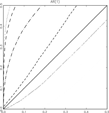
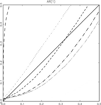
Figures 1 and 2 report the p-value plots for the case of ρu = ρz = 0.9. Figure 1 illustrates the p-value plots for the LMEL, unsmoothed KEL, smoothed KEL with [ell ]T = 2, unsmoothed K, and smoothed K with [ell ]T = 2 tests.11
We employ the truncated kernel for the kernel function k(·) and the Bartlett kernel for the HAC covariance estimator.
For the MA(1) case, we obtained similar results, but the magnitudes of overrejection for the unsmoothed tests were smaller than in the AR(1) case.

P-value plots for the LMEL (dashed), KEL (dotted), KEL with [ell ]T = 2 (short dashes), K (dots and dashes), and K with [ell ]T = 2 (closely spaced dots) tests.

P-value plots for the KEL tests with [ell ]T = 0 (dashed), [ell ]T = 2 (dotted), [ell ]T = 4 with [ell ]T = 6 (short dashes), and automatic [ell ]T (dots and dashes).
MATHEMATICAL APPENDIX
Notation.
Let C be a generic positive constant,

.
Proofs of the following lemmas are available from the author upon request.
LEMMA 1. Suppose that Assumptions 1 and 3–5 hold. Then

LEMMA 2. Suppose that Assumptions 1–5 hold. Then

LEMMA 3. Suppose that Assumptions 1 and 3–6(i)–(ii) hold. Then

LEMMA 4. Suppose that Assumptions 1–6 hold. Then

Proof of Theorem 1. The outline of the proof is similar to that of Theorem 5 of Guggenberger and Smith (2005a). Lemma 2(ii) implies that the FOC for

,

holds w.p.a.1. An expansion of (A.1) around

yields

, where

is a point on the line joining 0 and

. Lemmas 1(ii) and 2(i) and ρ2(0) = −1 imply that

. From Assumption 5(ii),

is invertible w.p.a.1, and

is written as

w.p.a.1. A second-order Taylor expansion of

around

yields

where

is defined similarly to

and the second equality follows from

and Lemma 2(iii). We next derive the asymptotic distribution of

. A similar argument for obtaining

implies that the derivative of (A.1) with respect to

converges in probability to a nonsingular matrix, −κ1Ω. Thus, applications of the implicit function theorem and the envelope theorem to (A.1) imply

. An expansion of (A.1) around

yields

, where (β,λ) is a point on the line joining

. By stacking these equations and using (A.2),

holds w.p.a.1, where

and

. Lemmas 1(ii) and 2(i) and (iii) and Assumption 1 imply that

. Assumptions 1(iii) and 5(ii) imply that A is invertible w.p.a.1. Thus, solving (A.4) for

yields

, where H ≡ (M2β′Ω−1M2β)−1M2β′Ω−1. An expansion of

around

and Lemma 2(iii) yield

where

is a point on the line joining

. From Lemma 1(iii) and Assumption 1,

. Therefore, from (A.3) and (A.5), we have

. █
Proof of Theorem 2. We follow the argument in the proof of Theorem 6 in Guggenberger and Smith (2005a). Let

. First, we show that

are asymptotically independent. Let M2α2 ≡ ∂m2(α02,β0)/∂α2′. An expansion of

around

, Lemmas 1(ii) and 2(i), and (A.2) yield

where the second equality in the second equation follows from Lemmas 2(iii) and 3(i) and

. An expansion of

around

(see the proof of Theorem 1) yield

where

is a point on the line joining

and the second equality follows from Lemma 2(iii) and

(by a similar argument as Lemma 3(i) using Assumption 6(ii)). From Lemma 3(ii), (A.5), and (A.6), stacking

yields

where

. Thus, from Lemma 3(iii),

is asymptotically normal with the asymptotic covariance matrix κ12ΨV(θaβ0)Ψ′. Because the asymptotic covariance of

(i.e., the off-diagonal component of κ12ΨV(θaβ0)Ψ′) is 0,

are asymptotically independent.
Next, we derive the asymptotic distribution of

. Lemma 4(ii) implies that the FOC for

,

holds w.p.a.1. An expansion of (A.8) around

yields

, where

is a point on the line joining 0 and

. By combining an argument similar to the proof of Theorem 6 in Guggenberger and Smith (2005a), Assumptions 1 and 6(i) and (ii), Lemma 3, and (A.7), we can show that

converges to a full column rank random matrix a.s. Thus, from

(by Assumption 6(iii) and Lemmas 1(ii) and 4(i)),

is invertible w.p.a.1 and

holds w.p.a.1. A second-order Taylor expansion of

around

yields

where

is defined similarly to

, the second equality follows from Assumption 6(iii) and Lemmas 1(ii) and 4(i), and the third equality follows from the FOC for

(i.e.,

and (A.2). From (A.7), we can denote

. By the inversion formula of partitioned matrices, the pα × pα upper left submatrix of the limit of

is [Dα′−1Ω−1Δ(θaβ0)Dα]−1. Therefore, the continuous mapping theorem and asymptotic independence of

imply that

where

. Also, from Assumption 1(ii), we have

. █
References
REFERENCES
Andrews, D.W.K.,
M. Moreira, &
J.H. Stock
(2004)
Optimal Invariant Similar Tests for Instrumental Variables
Regression.
Working paper,
Yale University.
Caner, M.
(2003)
Exponential Tilting with Weak Instruments: Estimation and
Testing.
Working paper,
University of Pittsburgh.
Davidson, R. &
J.G. MacKinnon
(1998)
Graphical methods for investigating the size and power of hypothesis
tests.
Manchester School
66,
1–26.Google Scholar
Guggenberger, P. &
R.J. Smith
(2005a)
Generalized empirical likelihood estimators and tests under partial,
weak and strong identification.
Econometric Theory
21,
667–709.Google Scholar
Guggenberger, P. &
R.J. Smith
(2005b)
Generalized Empirical Likelihood Tests in Time Series Models with
Potential Identification Failure.
Working paper,
University College London.
Guggenberger, P. &
M. Wolf
(2004)
Subsampling Tests of Parameter Hypotheses and Overidentifying
Restrictions with Possible Failure of Identification.
Working paper,
UCLA.
Jansson, M.
(2002)
Consistent covariance matrix estimation for linear processes.
Econometric Theory
18,
1449–1459.Google Scholar
Kitamura, Y.
(1997)
Empirical likelihood methods with weakly dependent processes.
Annals of Statistics
25,
2084–2102.Google Scholar
Kitamura, Y. &
M. Stutzer
(1997)
An information-theoretic alternative to generalized method of
moments estimation.
Econometrica
65,
861–874.Google Scholar
Kleibergen, F.
(2002)
Pivotal statistics for testing structural parameters in instrumental
variables regression.
Econometrica
70,
1781–1805.Google Scholar
Kleibergen, F.
(2005)
Testing parameters in GMM without assuming that they are
identified.
Econometrica
73,
1103–1123.Google Scholar
Moreira, M.J.
(2003)
A conditional likelihood ratio test for structural models.
Econometrica
71,
1027–1048.Google Scholar
Newey, W.K. &
R.J. Smith
(2004)
Higher order properties of GMM and generalized empirical likelihood
estimators.
Econometrica
72,
219–256.Google Scholar
Newey, W.K. &
K.D. West
(1994)
Automatic lag selection in covariance matrix estimation.
Review of Economic Studies
61,
631–654.Google Scholar
Smith, R.J.
(2004)
GEL Criteria for Moment Condition Models.
Working paper,
University College London.
Smith, R.J.
(2005)
Automatic positive semi-definite HAC covariance matrix and GMM
estimation.
Econometric Theory
21,
158–170.Google Scholar
Stock, J.H. &
J.H. Wright
(2000)
GMM with weak identification.
Econometrica
68,
1055–1096.Google Scholar
P-value plots for the LMEL (dashed), KEL (dotted), KEL with [ell ]T = 2 (short dashes), K (dots and dashes), and K with [ell ]T = 2 (closely spaced dots) tests.
P-value plots for the KEL tests with [ell ]T = 0 (dashed), [ell ]T = 2 (dotted), [ell ]T = 4 with [ell ]T = 6 (short dashes), and automatic [ell ]T (dots and dashes).
 You have
Access
- 36
- Cited by