


Introduction
Recent analyses of grave goods from British Chalcolithic and Early Bronze Age burials have demonstrated that the curation of significant artefacts was an important social practice (Sheridan et al. Reference Sheridan, Davis, Clark and Redvers-Jones2002; Woodward Reference Woodward2002; Hunter & Woodward Reference Hunter and Woodward2015). Often, this involved the deliberate fragmentation of objects such as necklaces and daggers as part of the funeral rite, a practice that may have allowed portions of such ‘heirlooms’ to be retained by the living (Jones Reference Jones, Jones and MacGregor2002; Brück Reference Brück2004, Reference Brück2019). Historically, discussion of Bronze Age mortuary rites has focused on practices—such as complete individual inhumation burials with associated grave goods—that appear to substantiate dominant social evolutionary narratives of growing complexity. Increasingly, however, it has been recognised that Bronze Age funerary practices were highly variable (Petersen Reference Petersen1972; Sofaer Derevenski Reference Sofaer Derevenski2002; Gibson Reference Gibson and Czebrezuk2004; Brück Reference Brück2006; Appleby Reference Appleby2013; Fowler Reference Fowler2013). Chalcolithic and Early Bronze Age burials often include partial or disarticulated skeletons. In some cases, for instance when disarticulated human bones are found strewn through the backfill of graves, these may have been accidentally redeposited from disturbed primary inhumations. In other cases, the representation of disarticulated skeletal elements, the manner of their modification and the nature of their deposition suggest levels of care indicating intentional deposition. The question, therefore, is whether human bones, like other artefacts, were deliberately curated in practices involving their fragmentation, circulation and redeposition over protracted periods.
Cremation burial was also common during the later Early Bronze Age and subsequent Middle Bronze Age (Ellison Reference Ellison, Barrett and Bradley1980; Caswell & Roberts Reference Caswell and Roberts2018). Deposits of cremated bone are often of insufficient weight to account for a whole individual (Brück Reference Brück2006, Reference Brück2009). Although this could be explained by the retrieval of only small quantities of cremated bone from the pyre, it is also possible that the cremated remains were divided between mourners for retention. Some cremation burials contain the burnt remains of multiple individuals. While contexts containing the remains of two or three individuals could be explained by simultaneous cremation, or cremation on the same pyre site, in certain cases the number of individuals represented is too high for this to be plausible. In these cases, it is more likely that cremation remains from several ceremonies had been accumulated intentionally.
During the Late Bronze Age and earliest Iron Age, fragments of disarticulated, unburnt bone, as well as small quantities of cremated bone, were frequently deposited in and around settlements, in roundhouses, waterholes and field boundaries (Brück Reference Brück1995). The patterning of the skeletal elements represented and the spatial distribution of these finds suggest that they were deliberate deposits. As yet, it is unclear whether such finds represent the endpoint of prolonged funerary rituals involving the defleshing, fragmentation and selective redeposition of certain remains, or systematic curation, in which disarticulated and cremated human bones were intentionally retrieved and preserved for substantial lengths of time before deposition. Continued interest in old objects during this period is indicated by the inclusion of ‘out-of-time’ artefacts in Late Bronze Age hoards (Knight Reference Knight, Knight, Boughton and Wilkinson2019).
The recognition of diversity in Bronze Age mortuary practices forms part of wider discussions around the significance of the dead and concepts of the body and the self in prehistory (Fowler Reference Fowler2010). The complexity of Neolithic mortuary deposits has been well described (e.g. Wysocki & Whittle Reference Wysocki and Whittle2000; Smith & Brickley Reference Smith and Brickley2009), and the architecture of Neolithic tombs often made it possible to retrieve human bone for manipulation, circulation and redeposition in other contexts. In the Iron Age, it has been argued that the skulls of enemies were curated and displayed in certain contexts (Armit Reference Armit2012), although the careful deposition of very old human remains suggests that rediscovered bones may sometimes have been venerated as ‘ancestors’ (Armit & Ginn Reference Armit and Ginn2007).
The primary question addressed in this article is whether radiocarbon dating can provide evidence for the systematic curation of unburnt and/or cremated human bone from the British Chalcolithic to the earliest Iron Age (2450–600 BC), hereafter referred to as the British Bronze Age. We then investigate how long any curated bones may have been kept before final deposition. Establishing the timescales for these practices will help us to understand how these remains may have been perceived by the communities to which they belonged, and, potentially, provide insight into the ideologies that drove these practices and imparted power to curated human remains. It is important to distinguish, for instance, whether bones could conceivably have come from the remains of someone that the community knew in life (i.e. a recent or known ancestor linked with a specific family or lineage) or someone from the distant past who existed beyond living or cultural memory (i.e. an anonymous or mythical ancestor connected more broadly to the entire community).
Unburnt disarticulated bones suitable for curation may have been obtained in a number of ways. First, corpses may have been dismembered and defleshed. Few Bronze Age human bones show cut marks indicative of such processes, but this is dependent on the skeletal representation or completeness of the deposited remains as well as the dexterity of the person processing the body (Fisher Reference Fisher1995). Second, disarticulated bones may have been exhumed from old primary burials. Third, excarnation (sub-aerial exposure of the body before burial) may have been practised. Evidence for this practice, normally consisting of patterns of carnivore modification and characteristic weathering (Carr & Knüsel Reference Carr, Knüsel, Gwilt and Hazelgrove1997; Smith Reference Smith2006), is however ambiguous, as its presence would be dependent on the nature of the rites (e.g. the amount of time that the defleshed bone was exposed to the elements, and the extent to which the environment was sheltered and the remains protected from scavengers). Histological analysis of British Bronze Age skeletons found evidence that some had been mummified and fragmented (Parker Pearson et al. Reference Parker Pearson2005; Booth et al. Reference Booth, Chamberlain and Pearson2015), making it plausible that disarticulated bones in other contexts represent the fragmented remains of bodies treated in this way. We will employ histological analysis to address aspects of the depositional histories of unburnt bones and to assess whether the treatment of the body may relate to any curation practices.
Radiocarbon dating
We generated 82 new radiocarbon dates at the Bristol Radiocarbon Accelerator Mass Spectrometer Facility for human remains (38 unburnt, 16 cremated), and for associated material from the same or related contexts (on 22 unburnt faunal bones, two burnt animal bones, three charcoal fragments and one hazelnut shell). The latter were taken to represent the date (or at least a terminus ante quem) of deposition. Although it is impossible to control entirely for the possibility that some of the human remains were accidental inclusions, we have attempted to mitigate against this possibility by sampling large fragments of bone that were plausibly recognisable as human (skulls and long bones) that had been placed on prepared surfaces rather than retrieved from fills or mixed dumps of material. Our samples were not geographically restricted, as we did not know how many relevant contexts we would find, and we needed to anticipate that radiocarbon dating would occasionally fail.
We have combined our dates with 121 previously published Bronze Age radiocarbon dates on disarticulated human remains, cremated human bone and associated materials, including remains, from three sites (Canada Farm, Windmill Fields and Cladh Hallan) showing evidence for mummification (Figure 1 & Table S1 in the online supplementary material (OSM); Parker Pearson et al. Reference Parker Pearson2005; Booth et al. Reference Booth, Chamberlain and Pearson2015; Smith et al. Reference Smith, Allen, Delbarre, Booth, Cheetham, Bailey, O'Malley, Pearson and Green2016). For three sites (Canada Farm, Wilsford G.58 and Stanton St Bernard) that yielded no datable associated material, or for which radiocarbon dating of associated material failed due to the poor collagen preservation, we have compared radiocarbon dates of potentially curated material against broad calendrical date ranges inferred by artefact typology. In cases where we had dates from the same stratigraphic context, we have assessed agreement indices and χ2 tests generated as part of the Combine function in OxCal 4.3 using the IntCal13 curve to test the hypothesis that the individual's date of death and deposition were contemporaneous (Ward & Wilson Reference Ward and Wilson1978; Bronk Ramsey Reference Bronk Ramsey2009; Reimer et al. Reference Reimer2013). In cases where we had dates from stratigraphically related contexts, we have used agreement indices generated by chronological modelling to assess how well dates from potentially curated material agreed with their stratigraphic positions (Haslett & Parnell Reference Haslett and Parnell2008). We have flagged anomalous dates when agreement indices fell below 60 (Tables S2–S3; Bronk Ramsey Reference Bronk Ramsey2009).
Map of British Bronze Age sites used in this study (figure by J. Brück).

A minority (n = 9) of the samples tested have produced dates after 600 BC. Post-Iron Age dates are provided in Table S1, but are not discussed in detail here. Of the 60 Chalcolithic, Bronze Age and Iron Age archaeological contexts tested, 26 (43 per cent) contained human bones that were anomalously older than the dates relating to their deposition (Figure 2). One of the contexts, a Chalcolithic burial from West Cotton in Northamptonshire, consisted of a collection of disarticulated human remains recovered from a shallow pit beneath the base of a grave containing a single articulated inhumation. It is difficult to determine whether the disarticulated bones had been intentionally deposited with the burial, or if the grave had been placed by chance over a Neolithic pit containing the disarticulated remains (Harding & Healy Reference Harding and Healy2013). The offset between the dates of the articulated skeleton and the disarticulated bones in this grave is a notable outlier, which, combined with the uncertain stratigraphic relationship, led us to exclude these results from further tests. In three cases, disarticulated faunal bone taken to reflect the date of deposition was anomalously older than the human bone, indicating either the incidental inclusion of old animal bones or the curation of old faunal remains.
Offset between pairs of radiocarbon determinations representing the death and deposition (or terminus ante quem) of human remains plotted against jittered median calibrated radiocarbon dates of deposition (see Table S3 in the online supplementary material; figure by T. Booth).

Omitting the anomalous West Cotton burial and the four later Iron Age contexts, 23 out of 55 Bronze Age bones (42 per cent) are anomalously too old (see Table S2 and Section 1 in the OSM). A series of statistical tests (detailed in the OSM, Section 1) indicate that there are significantly more anomalous results than expected in our sample, through all phases of the Bronze Age.
Figures 3–4 show unmodelled probability distributions for the differences between the dates of death and deposition of human remains for each context as an indication of the periods over which human remains were retained. Further distributions (intervals) are tested for differences between dates from human bones and associated material and compared against a control sample (Figure 5). In these tests too, the results indicate the presence of anomalously old human remains in our sample, consistent with the curation of human bone through the Bronze Age (OSM Section 1).
Unmodelled Differences (68 per cent confidence) between dates of death and the deposition of human remains from Bronze Age Britain plotted against jittered median calibrated dates of deposition (see Table S3 in the online supplementary material; figure by T. Booth).

Line graph showing variability in unmodelled Differences (medians and 68 per cent confidence ranges) between dates of death and deposition through the British Bronze Age (figure by T. Booth).

Violin plot showing kernel distribution of combined Bronze Age Intervals generated in BChron plotted alongside a normal distribution with the same sample size and standard deviation with a mean of 0. Kernel distributions were generated using the geom_violin function in the ggplot package in R Studio with default parameters (kernel = “gaussian”, bw = “nrd0”, scale = “area”; R Core Team 2013; figure by T. Booth).

We also note that Bronze Age Intervals that are not significantly anomalous are still slightly offset from a comparable control (Figure 6). Bronze Age human remains that were curated for decades or centuries would not always show up as anomalously old using the tests provided in OxCal (see OSM Section 1–2). We have therefore performed another test of our combined Bronze Age Intervals with all the anomalous Intervals removed against the control distribution described above. This Bronze Age distribution without anomalous dates was significantly older than the control and consistent with our hypothesis that this sample set probably includes curated human bones that do not show up in site-specific χ2 tests or agreement indices.
Violin plot showing kernel density of combined Bronze Age intervals generated in BChron, with significantly anomalous dates removed, plotted alongside a normal distribution with the same sample size and standard deviation with a mean of 0. Kernel distributions were generated using the geom_violin function in the ggplot package in R Studio with default parameters (kernel = “gaussian”, bw = “nrd0”, scale = “area”; R Core Team 2013; figure by T. Booth).

Radiocarbon dates from human remains can be significantly older than dates from their depositional context for a variety of reasons. If an individual obtained a large proportion of their dietary protein from marine or freshwater resources, for example, the accumulation of old carbon in bone collagen produces a ‘reservoir effect’, making any associated date look early (Lanting & van der Plicht Reference Lanting and van der Plicht1998). Fortunately, stable isotope analyses of human remains from Bronze Age Britain suggest that populations obtained very little of their dietary protein from marine or freshwater resources (Parker Pearson et al. Reference Parker Pearson2016). Δ13C values obtained on human bone as part of AMS radiocarbon dating for samples included here provide no evidence for a substantial marine reservoir effect (Table S1). Our own stable isotope values, along with some previously published values, however, have not been acquired on the standard isotope ratio mass spectrometer. Another possible source of error is that radiocarbon dates obtained from cremated human bone may not always represent an unadulterated signature corresponding to the date of death. Rather, carbon exchange between the bone and fuel during cremation means that the bone wholly or partially takes on the signature of the fuel. This could produce an ‘old wood effect’ if the fuel consisted of heartwood from a long-lived species, such as oak (Olsen et al. Reference Olsen, Heinemeier, Hornstrup, Bennike and Thrane2013; Snoeck et al. Reference Snoeck, Brock and Schulting2014).
We have analysed seven contexts where cremated remains represented the hypothesised curated material. Four produced anomalously early dates. It is unlikely that the low number of cremated bones included here would have had a major influence on the overall results. Cremated bones identified as significantly old were no older than unburnt bones producing significantly anomalous dates. We would expect that the old wood effect would produce a more uneven distribution of ages. While we cannot rule out the possibility that the old wood effect could be responsible for these anomalously old cremated bones, a scenario involving the curation of these bones is a plausible alternative (Olsen et al. Reference Olsen, Heinemeier, Hornstrup, Bennike and Thrane2013; Snoeck et al. Reference Snoeck, Brock and Schulting2014). Generally, the results of our analysis of the radiocarbon data are best explained by human remains having been curated and deliberately deposited years later.
The median of the combined Bronze Age intervals is 65 years older than the date of deposition, with an interquartile range of 183 (first quartile = −167, third quartile = 16). On average, therefore, curated human remains were deposited by people who lived around two generations after the individual's death, although it is possible that these bones could have come from an individual of the same generation or as many as six generations distant from the communities who finally deposited them. We produced alternative difference probability distributions within new phase models in OxCal 4.3, assuming that all the human remains we included had been curated and were older than the materials used to date their deposition (Figures 7–8). This produced artificial and idealised, but narrowed, intervals within younger ranges, emphasising that, in most cases, curation was probably on the younger end of the unmodelled distribution of intervals/generational timescales.
Modelled Differences (68 per cent confidence) between dates of death and deposition for Bronze Age human remains plotted against jittered median calibrated dates of deposition (see Table S3 in the online supplementary material; figure by T. Booth).

Line graph showing variability-modelled Differences (median and 68 per cent confidence ranges) between dates of death and deposition through the British Bronze Age (figure by T. Booth)

Our results suggest that Bronze Age human remains were curated for relatively short periods, from decades to around a century. In most or all cases, curated human bones probably represent the remains of individuals whose identity was known and who existed within living or cultural memory. It is possible that the final deposition of their remains took place when the individual was on the verge of passing out of social memory. The power of curated bones is likely to have lain in the identity of the individuals to whom they belonged, and their relationship to living persons, whether familial or otherwise. Our results are inconsistent with curated remains representing distant, unknown and perhaps mythical ancestors linked to entire communities.
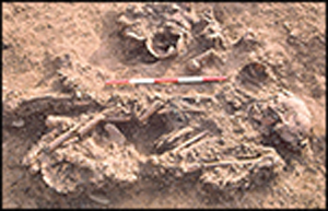
The Chalcolithic and Early Bronze Age human bones included here originate exclusively from funerary contexts. These old bones may represent the movement of human remains between different funerary deposits rather than curation practices per se, where human remains were retained amongst living communities. At Windmill Fields, Ingleby Barwick in North Yorkshire, the intact burial of an adult female (Sk 6) was accompanied by disarticulated crania and long bones representing at least three other individuals (Sk 8): a possible adolescent female, an adult male and an adult female (Figure 9; Annis et al. Reference Annis1997). The two adult crania are both anomalously older than the articulated burial, but contemporaneous with the excarnated, disarticulated human remains recovered from a wooden mortuary structure located a few metres away (Booth et al. Reference Booth, Chamberlain and Pearson2015). It seems reasonable to speculate that the disarticulated bones accompanying the articulated burial had been retrieved from the wooden cist and that this structure had acted as a cache of excarnated human remains that could be used in later funerary rituals. If the remains of the dead were viewed as powerful or significant by living communities, all Chalcolithic and Early Bronze Age burials may have represented potential caches of bone.
Inhumation Sk 6 from Windmill Fields, Ingleby Barwick, North Yorkshire, accompanied by Sk 8 comprising the disarticulated remains (mostly skulls and long bones) of an additional three individuals (image provided courtesy of Tees Archaeology).

The recovery of curated remains from Middle and Late Bronze Age settlements in Britain suggests that human bone may also have circulated among the living over protracted periods of time. At Striplands Farm in Cambridgeshire, cremated human bone was deposited in a pit that formed part of a Late Bronze Age settlement (Evans et al. Reference Evans, Patten, Brudenell and Taylor2011); this was 7–89 years older (at 68 per cent confidence) than burnt animal bone from the same context. Curated human bone may have had particular potency when incorporated into deposits relating to the identity and life cycle of the household group, such as foundation or abandonment deposits (Brück Reference Brück1999, Reference Brück2006). Yet, variability in the timeframes over which human bone was curated suggests that it may have been retained for many different reasons. The disarticulated frontal bone of an adult male retrieved from a pit at Eye Quarry in Cambridgeshire exhibited a probable blade injury (Patten Reference Patten2004). The radiocarbon date from this bone was statistically consistent with that of an animal bone deposited in the same context. The skull fragment is therefore unlikely to have been curated over a long period (e.g. decades or centuries), although it may nonetheless have been displayed for a time (perhaps months or years) as a means of humiliating and intimidating a perceived enemy.
Histological analysis
Bacterial bioerosion of internal bone microstructures varies in ways that correspond to early post-mortem treatment, probably because bioerosion relates in some way to soft tissue decomposition (Jans et al. Reference Jans, Nielsen-Marsh, Smith, Collins and Kars2004; Nielsen-Marsh et al. Reference Nielsen-Marsh, Smith, Jans, Nord, Kars and Collins2007; Booth Reference Booth2016). Patterns of bacterial attack can indicate the variety of taphonomic trajectories represented in a given assemblage (Booth & Madgwick Reference Booth and Madgwick2016). The relationship between how bacterial bioerosion varies in skeletal remains from different archaeological and forensic contexts, as well as broader models of bodily decomposition, can then be used to infer specific funerary rites. Previous analysis of bacterial bioerosion patterns in British Bronze Age human remains have revealed a bimodal distribution in the levels of attack: around half showing high levels of bioerosion—which is most consistent with primary burial—and half showing little or no bacterial attack, which is most consistent with mummification or excarnation (Booth et al. Reference Booth, Chamberlain and Pearson2015).
Seventeen Bronze Age human bones sampled for radiocarbon dating as part of the current study were also subject to histological analysis using non-destructive micro-computed tomography (micro-CT). This was conducted to investigate levels of bacterial bioerosion to infer diversity in patterns of treatment and to investigate relationships with curation practices (OSM Section 3). Levels of bacterial bioerosion were assessed by the analysis of virtual transverse slices using the Oxford Histological Index (OHI; Hedges et al. Reference Hedges, Millard and Pike1995; Millard Reference Millard, Brothwell and Pollard2001). Six samples show high levels of bacterial bioerosion (OHI<2), while the other 11 show little or no bacterial attack (OHI>4; Table S5; Figure 10). This bimodal distribution of OHI scores resembles that recorded previously for British Bronze Age human remains (Booth et al. Reference Booth, Chamberlain and Pearson2015). Our results suggest that at least two taphonomic trajectories are represented amongst the disarticulated remains analysed here, probably reflecting distinct funerary treatments.
Vase plot showing kernel density and distribution of Oxford Histological Index (OHI) scores for Bronze Age samples that were analysed histologically. They show a bimodal distribution at the extremes of the OHI scale. Kernel distributions were generated using the geom_violin function in the ggplot package in R Studio with default parameters (kernel = “gaussian”, bw = “nrd0”, scale = “area”; R Core Team 2013; figure by T. Booth).

High levels of bacterial attack are most often found in the bones of articulated skeletons that were originally buried as intact bodies soon after death (Jans et al. Reference Jans, Nielsen-Marsh, Smith, Collins and Kars2004; Nielsen-Marsh et al. Reference Nielsen-Marsh, Smith, Jans, Nord, Kars and Collins2007; Booth Reference Booth2016). The Bronze Age samples in this study showing high levels of bioerosion were probably exhumed from primary burials, post-skeletonisation. Anoxic or waterlogged environments inhibit osteolytic bacteria (Turner-Walker & Jans Reference Turner-Walker and Jans2008; Booth Reference Booth2016). Six of the eleven bones showing low or no bacterial attack originate from contexts—usually ancient waterholes—that were probably waterlogged over the period of deposition, at least episodically. The disarticulation of these remains, however, suggests that these environments did not represent the primary depositional context; hence the waterlogged conditions, being secondary, are unlikely to have affected early bodily decomposition. Moreover, there is no indication that most of these contexts were waterlogged when they were excavated. Bones from periodically inundated environments tend to exhibit variable levels of bacterial attack (Booth Reference Booth2016). This does not correspond to what we have observed in the histologically well-preserved Bronze Age remains examined here, where bacterial bioerosion is usually slight or absent. Early post-mortem treatment is more likely to be responsible for the levels of bioerosion in the samples analysed, particularly given that the patterns of bioerosion are similar to those observed previously in Bronze Age British remains from aerobic, dry contexts (Booth et al. Reference Booth, Chamberlain and Pearson2015).
Bones from aerobic contexts showing low levels of bacterial attack are usually those that were subjected to funerary rites which had rapidly removed soft tissue, such as dismemberment, defleshing and excarnation, or rites that inhibited bodily decomposition, such as mummification (Jans et al. Reference Jans, Nielsen-Marsh, Smith, Collins and Kars2004; Nielsen-Marsh et al. Reference Nielsen-Marsh, Smith, Jans, Nord, Kars and Collins2007; Booth et al. Reference Booth, Chamberlain and Pearson2015; Booth Reference Booth2016). None of the bones sampled here show evidence for cut marks indicative of defleshing or dismemberment; the simplest explanation is that they came from bodies that had been excarnated.
There is no temporal patterning in our histological results, suggesting that bodies could have been subject to primary burial or excarnation during all phases of the Bronze Age in Britain. There was no relationship between the radiocarbon evidence for bones having been curated and early post-mortem treatment as indicated by levels of bacterial bioerosion. It seems that most people were given specific funerary treatment that was deemed appropriate, and that the decision to retain, retrieve and curate bones was made at a later stage.
Conclusions
A high proportion of unburnt disarticulated human remains and burnt human bone recovered from British Bronze Age contexts and analysed here were probably already ‘old’ when they were deposited, providing the first clear evidence for systematic curation of human bones in this period. The duration of curation was fairly short: a few decades on average, and up to around 200 years at most. These timescales suggest that the individuals represented by these remains had lived approximately two generations before the communities who eventually deposited their bones, and could have existed within living or cultural memory. These remains were probably those of known individuals, kept by people or groups who had a defined relationship with the deceased; these relationships may have endowed the curated bone with its meaning and power. Our results reject a scenario in which remains represent anonymous or mythic distant ancestors linked to entire living communities.
In the Chalcolithic and Early Bronze Age, these ‘old’ bones may not represent curation amongst the living, but significant remains retrieved from extant graves or repositories to accompany new burials—although synchronous evidence for excarnation complicates this scenario. For the Middle to Late Bronze Age and earliest Iron Age, many of our samples were recovered from settlement contexts. Their deposition may be the end-point of complex trajectories in which human remains were curated amongst the living. Our analysis of bone diagenesis shows no clear links between funerary treatment and curation, suggesting that these practices were separate. Our study adds to the evidence for excarnation and the remarkable complexity of mortuary behaviour in Bronze Age Britain as well as to ongoing discussions around the power and significance of the dead in prehistory. It also contributes to debates concerning the importance of relational forms of personhood, as it suggests that the links between the living and the dead were central to the construction of Bronze Age social identities.
Acknowledgements
This research was funded by a grant from the Gerda Henkel Foundation (AZ 04/F/15). We are extremely grateful to Tim Knowles and Paul Monaghan (Bristol Radiocarbon AMS laboratory), and to Rui Martiniano for his help with R statistical computing. We would like to thank all those responsible for providing access to samples and contextual information on deposits: Lauren McIntyre and Fraser Brown (Oxford Archaeology South); Natasha Dodwell (Oxford Archaeology East); Chris Evans, Marcus Brittain, Justin Wiles, Mark Knight and David Gibson (Cambridge Archaeology Unit); Robin Daniels (Tees Archaeology); Jacky Nowakowski (Cornwall Archaeology Unit); Phil Andrews and Kirsten Egging-Dinwiddy (Wessex Archaeology); James Harris and Alison Brookes (Corinium Museum); Dave McOmish and Simon Mays (Historic England); John Barrett (University of Sheffield); Chris Fowler and Michelle Gamble (Newcastle University); Steve Minnitt, Richard Brunning and Amal Khreisheh (Somerset Heritage Centre); David Dawson and Lisa Brown (Wiltshire Museum); Hannah Cutler (Suffolk County Council); Stefanie Vincent (Swindon Museum); Sharon Clough (Cotswold Archaeology); and Alex Croom (Arbeia Museum). Thanks also to Peter Marshall for the method of calculating radiocarbon date offsets. We are grateful to the three anonymous reviewers whose constructive comments helped to improve this paper considerably.
Supplementary material
To view supplementary material for this article, please visit https://doi.org/10.15184/aqy.2020.152



