1. INTRODUCTION
Motion planning is ubiquitous in many geometrically intensive applications involving moving objects such as robotics, virtual reality, computer graphics, computer-aided design, and manufacturing, computer-aided surgery, computational biology, and many others. It heavily relies on spatial information about the environment in which the navigation takes place, and typically focuses on generating a “useful” motion that takes a moving object, a robot, or a vehicle, between two prescribed configurations subject to some constraints such as minimum length of the path, collision-free trajectories, and intermediate sites.Footnote 1 One of the most useful and common abstractions of this problem is to transform the motion planning of an object in the Euclidean space into the path planning of a point in the configuration space (or C-space) of the object (Latombe, Reference Latombe1991).
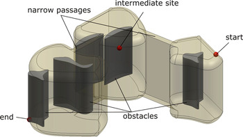
Consider a moving object leaving from an initial position and moving in the Euclidean space E d(d = 2, 3) toward a prescribed final destination. Such a vehicle can be a mobile robot, an autonomous vehicle, a camera flying through a scene, or collection of spatial entities,Footnote 2 a mechanical part that is being assembled or transported, and so forth. The object may be constrained by intermediate sites that must be either approached or avoided during the motion, such as a fueling/loading/unloading station or a sightseeing location. The environment itself can be static or dynamic, case in which the obstacles themselves or the boundary of the environment are changing during the motion. The task is to find a path from start to finish that satisfies the intermediate site constraints and is subjected to other specific constraints as illustrated in Figure 1. In its most general form, finding a path in such an environment is a hard problem. Consequently, the existing approaches address simplified versions of this problem.
An object moving in an evolving environment with one intermediate site that must be approached during the motion. [A color version of this figure can be viewed online at journals.cambridge.org/aie]

A large amount of research has been devoted to motion planning in static environments with both exact and approximate methods. The existing approaches for finding the motion, which cannot be easily extended to dynamic environments, can be classified into the following:
1. roadmap methods that plan curves in either the configuration space of the moving object or in the Euclidean space in which the object moves. There has been some success in constructing three-dimensional (3-D) configuration spaces (see, e.g., Sacks et al., Reference Sacks, Pisula and Joskowicz1999), but computing C-spaces explicitly remains a difficult problem, which is exponential in the number of dimensions of the C-space (Latombe, Reference Latombe1991). Consequently, computing roadmaps in the Euclidean space has remained a strong area of research. Current motion planning algorithms that compute roadmaps rely on visibility graphs (Jiang et al., Reference Jiang, Seneviratne and Earles1999; Neus & Maouche, Reference Neus and Maouche2005), Voronoi diagrams (Diaz de León & Sossa, Reference Diaz de León and Sossa1998; Wilmarth et al., Reference Wilmarth, Amato and Stiller1999; Foskey et al., Reference Foskey, Garber, Lin and Manocha2001; Garber & Lin, Reference Garber and Lin2002; Lee & Choset, Reference Lee and Choset2005; Geraerts & Overmars, Reference Geraerts and Overmars2007), silhouette curves of semialgebraic sets (Canny, Reference Canny1993), or probabilistic roadmap planners (Kavraki et al., Reference Kavraki, Vestka, Latombe and Overmars1996);
2. potential field methods that introduce artificial attractive/repulsive field in the environment can conceptually handle both static and moving obstacles (Rimon & Koditschek, Reference Rimon and Koditschek1992; Xidias et al., Reference Xidias, Azariadis and Aspragathos2007). These methods cannot take into consideration the exact geometry of the obstacles, and therefore they cannot be applied to those problems in which the moving object is moving in close proximity with the obstacles. It is of more importance that potential field methods introduce local minima of the potential field that can “trap” the moving object;
3. approaches based on cell decompositions, which are inherently approximate. These methods perform a disjoint decomposition of the free space, construct the connectivity graph connecting these cells, and perform graph search algorithms to select a collision free path (Choset, Reference Choset2000; Lingelbach, Reference Lingelbach2004).
An approximately time-optimal trajectory is proposed in van den Berg and Overmars (Reference van den Berg and Overmars2005) that uses a precomputed roadmap for the static part of the scene to determine the collision-free trajectory among the moving obstacles. This approach requires the complete environment and motions to be known ahead of time. Other approaches that incorporate into the formulation time as the extra dimension have been discussed in Ishikawa (Reference Ishikawa1991) and Fraichard (Reference Fraichard1993). More general approaches to dynamic motion planning couple a precomputed probabilistic road map and a cell decomposition to dynamically determine which cells of the roadmap are affected by the motion of the obstacles (Kallman & Mataric, Reference Kallman and Mataric2004). These methods produce successful paths when the dynamic subset of the environment is much smaller than the whole environment, and when changes to the precomputed roadmap are fairly minor. Motion planning in dynamic environments in which both moving obstacles and target are moving with known velocities has been addressed in Masehian and Katebi (Reference Masehian and Katebi2007). Because of the assumption of known velocity vectors, this approach cannot handle the case when the number, type, and motion of the moving obstacles are not known in advance.
A fast motion planning algorithm in a two-dimensional (2-D) dynamic environment based on generalized Voronoi diagrams has been described in Hoff et al. (Reference Hoff, Culver, Keyser, Lin and Manocha2000). The Voronoi decomposition is computed for the prescribed “sites”—the obstacles of the domain. For each pixel in the domain they compute the closest site and shortest distance to that site. All pixels closest to the same site get assigned the same color so that different Voronoi cells will have different colors. The algorithm has been implemented on the graphics processing unit, which allows the computation of the Voronoi decomposition at each time step.
1.1. Main contributions of our work
In this paper we present a strategy to develop a family of paths, or roadmaps, for 2-D and 3-D solidsFootnote 3 moving in highly dynamic environments that can undergo drastic topological changes. The main contribution of this paper is the definition of a class of skeletons that have the same homotopy as that of the environment and contains the medial axis as a special case. It is important that our skeletons can be designed so that they are attracted to or repulsed by prescribed sites in the environment, whereas the attraction and repulsion are controlled by a set of degrees of freedom (see Section 2.6). This can effectively alter the planned path to accommodate specific geometric constraints such as approaching a refueling station or a sightseeing location. Furthermore, we exploit the concept of a medial zone that we introduced in Eftekharian and Ilieş (Reference Eftekharian and Ilieş2010) to control the subset of the environment in which the roadmaps are being computed, and we show that, for the same domain, the resulting roadmaps are shorter and smoother than those obtained based solely on skeletons.
Once we construct the corresponding skeletons and medial zones, we use the established Dijsktra's algorithm to compute shortest paths of moving points along the skeletons or within the medial zones. Furthermore, the properties of R-functions afford a conservative motion planning of solid objects within the same formulation via level sets. The approach presented in this paper can handle problems in which one or more objects move in environments that are not fully known in advance, and intrinsically supports local and parallel computations of skeleton and medial zones (and, hence, path planning) for domains with rigid or evolving boundaries. Our approach can be implemented in any commercial geometric kernel, and has attractive computational properties.
2. PROBLEM FORMULATION
In this paper we focus on evolving spatial environments with obstacles that can move as well as merge/split. We assume that the initial and final position (i.e., points in the environment) of the path to be planned are known, and that two lists of obstacles that contain the “attractive” obstacles  as well as “repulsive” obstacles ℛ are provided along with positive parameters λ ∈ ℝ+ that quantify the extent by which each obstacle will attract or repulse the path to be computed (see Section 2.6). Each site that must be approached is specified by the user. The task that we investigate in this paper is to compute the shortest path along the skeleton or within the medial zones that connects the prescribed initial and final positions subject to the intermediate constraints, or output a message that one does not exist for the prescribed environment.
2.1. Summary of the approach
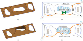
Our approach is illustrated in Figure 2 and consists of five, not necessarily sequential, stages:
1. Construct an exact or approximate distance function over the given semianalytic domain.
2. Adjust the distance function according to the “attractive” and “repulsive” factors for obstacles prescribed in
 and ℛ.
3. Extract the skeleton of the domain as the subset of points where the continuous distance function is nondifferentiable. Note that our construction provides an explicit mapping between each half-space defining the environment and each branch of the skeleton, which can play a critical role in local skeleton computations.
4. Alternatively, compute the medial zones as “thick” versions of the skeletons;
5. Compute the shortest collision free path along the skeleton or inside the medial zones subject to the intermediate sites that must be visited.
 and ℛ.
(a) The three-dimensional distance function of the domain constructed with R-functions, (b) the medial axis of the domain and the shortest path that follows the medial axis of the domain, and (c) the modified skeleton attracted to the intermediate target and the resulting shortest path. [A color version of this figure can be viewed online at journals.cambridge.org/aie]

Steps 1 and 3 above are summarized in Section 2.2 (see also Eftekharian & Ilieş, Reference Eftekharian and Ilieş2009); step 2 is discussed in Section 2.3, whereas the medial zones are summarized in Section 3 and described in detail in Eftekharian and Ilieş (Reference Eftekharian and Ilieş2010). Section 4 illustrates the usefulness of our approach for several domains that simulate highly dynamic, topologically evolving domains.
2.2. Preliminaries
Geometric skeletons are fundamental concepts in practically all geometrically intensive areas of science and engineering, such as automated finite element meshing, shape manipulation, recognition, and comparison, dimensional reduction in design and analysis, robotic surgery, and a variety of path and motion planning in commercial and defense applications. More recently, skeletons have been used to explore the fundamental geometric problems of folding and unfolding that are the abstraction of some of the most important open problems in science today, such as protein folding, as well as packing and sheet metal bending. There are multiple ways to define a skeleton of a given set, and a variety of definitions have been proposed for different applications. Introduced by Blum (Reference Blum1967) as a tool for image analysis, the medial axis has become one of the mainstream geometric concepts due to the fact that it provides a compact representation of the geometric features of a shape and its topology. The medial axis captures the connectivity of the shape, has a lower dimension than the space itself, and is closely related to the distance function constructed over the same domain.
The concept of medial axis has been described with the help of the fire grass concept (see, e.g., Attali et al., Reference Attali, Boissonnat, Edelsbrunner, Möller, Hamann and Russel2008) as follows: if a fire starts from all points of a planar curve at the same time and moves with constant velocities in all directions in the same plane, then the medial axis is the locus of points where the fire (in fact, a moving front) meets itself. The concept can be extended to k-dimensional geometric shapes in ℝk, case in which the medial axis becomes a set of dimension k − 1. Intuitively, the points on the medial axis are equally distant to at least two points of the boundary of the domain. Since its formulation, the medial axis has been used as alternative solid modeling representation (Shaham et al., Reference Shaham, Shamir and Cohen-Or2004), as well as in many other applications such as shape matching and reconstruction (Liu et al., Reference Liu, Geiger and Kohn1998; Siddiqi et al., Reference Siddiqi, Shokoufandeh, Dickinson and Zucker1999; Sebastian et al., Reference Sebastian, Klein and Kimia2004; Damon, Reference Damon2005; van Eede et al., Reference van Eede, Macrini, Telea, Sminchisescu and Dickinson2006; Goh, Reference Goh2008), dimensional reduction in boundary value problems (Suresh, Reference Suresh2003), representation and classification of 2-D shapes (Sherbrooke et al., Reference Sherbrooke, Patrikalakis and Brisson1995; Pizer et al., Reference Pizer, Siddiqi, Székely, Damon and Zucker2003; Shah, Reference Shah2005), human vision (Kimia & Tamrakar, Reference Kimia and Tamrakar2002), pattern analysis and shape recognition (Blum & Nagel, Reference Blum and Nagel1978; Bookstein, Reference Bookstein1979), mesh generation (Sampl, Reference Sampl2000, Reference Sampl2001; Quadros et al., Reference Quadros, Shimada and Owen2004), and so forth.
The mathematical properties of medial axis are fairly well understood (Choi et al., Reference Choi, Choi and Moon1997; Chazal and Soufflet, Reference Chazal and Soufflet2004; Attali et al., Reference Attali, Boissonnat, Edelsbrunner, Möller, Hamann and Russel2008). However, the practical uses of these skeletons are limited by their notorious computational difficulties, and their instability under small perturbations of the shape. Although it is possible, in principle, to compute the medial axis exactly for general semialgebraic/analytic sets, we do not seem to have any algorithms for doing so. The most advanced algorithms make significant simplifying assumptions on the geometry of these sets by focusing on planar or piecewise linear shapes. Algebraic planar curve segments whose bisectors admit rational parametrizations are examined in Ramamurthy and Farouki (Reference Ramamurthy and Farouki1999), whereas exact computation of medial axis for polyhedra is described in Culver et al. (Reference Culver, Keyser and Manocha2004). The reasons behind these restrictions become apparent once the algebraic difficulties in computing medial axis (MA) are examined (Attali et al., Reference Attali, Boissonnat, Edelsbrunner, Möller, Hamann and Russel2008).
Consequently, these difficulties promoted a variety of algorithms that approximate the complex shape by a set bounded by a piecewise linear boundary for which the medial axis can be computed exactly, followed by the extraction of the medial axis of the approximating shape—the so-called pruning step. The computed medial axis has to be postprocessed in order to eliminate the branches that appear in the medial axis due to the shape approximation. The main approaches to approximately compute the medial axis for piecewise linear shapes rely on: Voronoi/Delaunay decompositions of space (Brandt & Algazi, Reference Brandt and Algazi1992; Amenta et al., Reference Amenta, Choi and Kolluri2001; Dey et al., Reference Dey, Woo and Zhao2003) where the medial axis is the Voronoi graph defined by a piecewise linear approximation of the shape (Attali et al., Reference Attali, Boissonnat, Edelsbrunner, Möller, Hamann and Russel2008); solutions of partial differential equations (such as diffusion or Hamilton–Jacobi equations; Siddiqi et al., Reference Siddiqi, Bouix, Tannenbaum and Zucker2002; Du & Qin, Reference Du and Qin2004); and level set methods (Kimmel et al., Reference Kimmel, Shaked, Kiryati and Bruckstein1995; Gomes & Faugeras, Reference Gomes and Faugeras2000). A recent method to compute the medial axis for curved planar sets (Cao & Liu, Reference Cao and Liu2008) is iteratively tracing the Frenet frames for pairs of boundary curves that bound a closed planar domain. This algorithm does not generalize to 3-D space and its stability appears to be problematic in 2-D due to its iterative marching along the boundary curves.
2.2.1. R-functions as logic operators on real-valued half-spaces
For any closed subset Ω of  d, one can construct a C ∞ function that vanishes on the boundary ∂Ω of Ω. It is known that such shapes are in fact semianalytic sets of points that can be constructed as a finite Boolean combination of real analytic functions f i ≥ 0. This in turn suggests an approach to construct a C n function over a semianalytic subset Ω of
 d by subdividing the boundary of Ω in primitive half-spaces f i, followed by a combination of f i into a single predicate using the standard Boolean logic operators AND, OR, or NOT (Shapiro, Reference Shapiro2007).
R-functions have been invented in the 1960s by V.L. Rvachev, who called these functions “logically charged functions.” These functions provide the means to construct a C n function over a domain defined by primitive half-spaces. The main contribution of the theory of R-functions to the topic of this paper is to replace these logical operations by real-valued functions, which generates an implicit representation for any semianalytic set Ω. One important feature of these real valued functions is that their sign is completely determined by the sign of their arguments, and is independent of any of their magnitudes.
There are many systems of sufficiently complete R-functions. One such system is known as principal system of R-functions

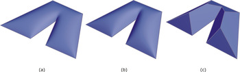
where (+) and (−) signs correspond to the R-conjunction (x 1 ∨αx 2) and R-disjunction (x 1 ∧αx 2) respectively of two real variables x 1 and x 2. By varying the value of α, we obtain different systems of R-functions. In particular, by setting α = 1 in Eq. (1) we obtain the R 1(Δ) system of R-functions, whereas a value α = 0 in Eq. (1) would result in the R 0(Δ) system (see Fig. 3).
Three implicit representations of a polygonal domain that correspond to (a) α = 0, (b) α = 0.5, and (c) α = 1. [A color version of this figure can be viewed online at journals.cambridge.org/aie]

Of importance, when expression under the square root in Eq. (1) becomes zero, the corresponding implicit function becomes nondifferentiable. Because the medial axis of a semianalytic domain corresponds to the points where the distance function is nondifferentiable, we will be looking for points of the implicit function where the expression under the square root vanishes.
Figure 3 shows the difference between the implicit functions constructed over a polygonal domain with the R α(Δ) system for three values of α. One can see that for α ≠ 1, the resulting functions are differentiable (except at the origin, not shown). In contrast, the implicit function corresponding to R 1(Δ) shown in Figure 3c is made of piecewise planar patches that intersect at piecewise linear edges. In fact, by projecting the edges of the R-function surface on the plane of the polygon we obtain a skeleton of the polygon. However, how do we construct the function, and which skeleton do we obtain?
2.2.2. Constructing Boolean expressions
Conceptually, the problem of constructing a Boolean expression for a domain bounded by half-spaces is the same as that of converting a boundary representation (B-rep) into a constructive solid geometry (CSG) representation in solid modeling.
Several efficient algorithms for performing the B-rep to CSG conversion for polygons are known (Tor & Middleditch, Reference Tor and Middleditch1984; Dobkin et al., Reference Dobkin, Guibas, Hershberger and Snoeyink1988). However, the complexity of the problem quickly escalates with the increase in the complexity of the boundary of the domain. Separating the boundary into primitive pieces is no longer sufficient to construct the Boolean expression of the domain, because additional half-spaces need to be introduced, which are the so-called separating half-spaces. Determining a sufficient set of separating half-spaces is the critical step of any such algorithm, but the problem is not well understood in general. Solutions exist for planar domains bounded by linear and curved edges that are subsets of convex curves (Shapiro, Reference Shapiro2001) and solids bounded by linear or quadric surfaces (Shapiro & Vossler, Reference Shapiro and Vossler1993).
Note that the problem of B-rep to CSG conversion is well defined by using the natural half-spaces of the domain, but a CSG expression may not exist for a given set of half-spaces. This necessary and sufficient condition for the existence of a CSG expression is formally described by the describability theorem” in Shapiro and Vossler (Reference Shapiro and Vossler1991). However, if a canonical CSG expression exists for a given set of half-spaces bounding a specific domain, then this canonical CSG expression is unique. Observe that we do not require the canonical CSG expression, because all CSG expressions that are valid for a given domain will describe the same set of points.
Planar domains
The Boolean set representation of a polygonal domain can be computed based on the convex deficiency tree (Dobkin et al., Reference Dobkin, Guibas, Hershberger and Snoeyink1988), which treats each polygon as its convex hull minus a finite number of concavities. Note that the polygon is a closed set, so the subtraction of concavities must necessarily be regularized (i.e., one must use regularized Boolean operations). Finally, we perform a syntactic substitution to replace the union and intersection with the R-disjunction and R-conjunction given in Eq. (1), which results in an R-function expression whose zero set is the original planar domain. By following this procedure, we obtain an R-function expression that corresponds to the exact distance function for any convex planar domain polygon, and an approximate distance function for a concave domain. Note that such a distance function is obtained from the principal system of R-functions given in Eq. (1) by setting the value of α = 1, that is, the R 1(Δ) system. Values of α < 1 correspond to implicit functions over the same domain that have established differential properties (Shapiro, Reference Shapiro2007). These approximate distance functions can be converted into an exact distance function by introducing additional half-spaces at the concave vertices of the domain (Eftekharian & Ilieş, Reference Eftekharian and Ilieş2009). Specifically, each concave vertex requires a conical half-space with a half angle of π/4 and two separating/trimming half-spaces that are normal to the boundary curves that are incident at the concave vertex.
3-D domains
It is important to note that the construction algorithms for simple polygons can be extended to some other point sets, such as curved polygons (Shapiro, Reference Shapiro2001), 3-D polyhedra, and more general 3-D solids (Shapiro, Reference Shapiro1991; Buchele & Crawford, Reference Buchele and Crawford2003). However, converting the resulting approximate distance function into an “exact” distance function for such domains requires the computation of additional halfspaces as discussed above, which can only be computed approximately in many situations. The alternative that we take in this paper is to compute distance functions to each face bounding the 3-D domain, and combine them with the R-disjunction as described in more detail in Eftekharian and Ilieş (Reference Eftekharian and Ilieş2010).
2.2.3. Adding/removing obstacles
Obstacles in the environment can be represented as holes/voids of the domain. One of the main advantages of our approach to compute skeletons based on R-functions is that obstacles can be easily added to the R-function expression representing Ω (see also Eftekharian & Ilieş, Reference Eftekharian and Ilieş2009). The R-function expression corresponding to the obstacle is subtracted from the R-function expression defining the boundary of Ω according to the R-subtractionFootnote 4

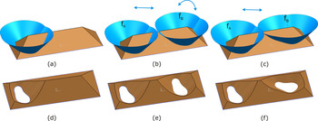
where f 1 is the function describing the outer domain and f 2 represents the hole. Figure 4 shows how obstacles can be added to the main space. Figure 4a–c illustrates this process in which two obstacles are sequentially added to the environment, then one of them is rotated. The corresponding distance functions are illustrated in Figure 4d–f.
Obstacles can be added to (or removed from) the environment. (a)–(c) Distance functions to individual obstacles are illustrated, and (d)–(f) the resulting distance functions of the domain are shown. [A color version of this figure can be viewed online at journals.cambridge.org/aie]

One important property of the R-functions is that their sign is independent of the magnitude of each half-space involved in the R-function expression, and depends only on the sign of each half-space. Consequently, holes can be easily relocated and resized to perform, for example, parametric or topology optimization (Chen et al., Reference Chen, Shapiro, Suresh and Tsukanov2007; Luo et al., Reference Luo, Tong, Wang and Wang2007). These modifications exploit the connection between implicit functions defined with R-functions and level sets so that the boundary of the domain defined by the R-function expression is the zero level set of the corresponding implicit function, and moving boundaries of Ω can be handled as easily (Eftekharian and Ilieş, Reference Eftekharian and Ilieş2009).
2.3. From distance functions to collision-free trajectories
Constructing the R-function expression described above results in the distance function of any 2-D or 3-D bounded, regular, closed and semianalytic domain. The ridges of the distance function contain the points where the distance function is nondifferentiable, and therefore, belong to the medial axis of the domain.
In Eftekharian and Ilieş (Reference Eftekharian and Ilieş2009) we explored two strategies for extracting the ridges of the distance function. Specifically,
1. for the planar case, if the distance functions H i corresponding to each individual half-space f i are constructed in a commercial geometric kernel as a standard 3-D NURBS surface, then the distance function corresponding to domain Ω can be obtained by combining the individual H i according to the Boolean expression developed in the previous step. This outputs individual curve segments/branches of the medial axis.
2. Alternatively, one can take advantage of the fact that the distance function is not differentiable at the ridge points. If one assumes that the first derivative of a given continuous function is large (it reaches a local extremum) wherever the second derivative has a zero crossing, one can use Laplacian based methods for ridge detection, which are widely used in image analysis and computer vision. This leads to a numerical procedure that outputs points of the medial axis, which needs to be followed by a segmentation of these points into branches of the medial axis. One practical way to perform the medial axis segmentation (or branching) is to determine the half-spaces H i that evaluate to zero for each point of the medial axis. The advantage of this approach is that it can be applied to both 2-D and 3-D path planning problems.
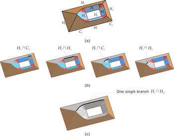
Regardless of the ridge extraction algorithm being employed, by constructing a single function describing the boundary of each obstacle we can significantly reduce the number of branches of the medial axis, which will significantly reduce the computational cost of the path planning algorithm. This is illustrated in Figure 5, which shows a polygonal domain and its exact distance function in Figure 5a. The rectangular obstacle is bounded by four half-spaces H 1, … , H 4, to which we add trimmed conical half-spaces C 1, … , C 4. These half-spaces can be treated individually or collectively during the segmentation, as mentioned above. Note that even though we use linear half-spaces for illustrative purposes, the approach remains valid for all semianalytic half-spaces.
Combining the half-spaces defining the obstacles into a single function reduces the number of branches of the medial axis. [A color version of this figure can be viewed online at journals.cambridge.org/aie]

If each individual half-space bounding the obstacle is treated individually during the segmentation, then one half-space defining the outer boundary of the environment, say H 5, will generate four separate branches of the medial axis as shown in Figure 5b. Alternatively, if we construct one single Boolean expression H o for the boundary of the obstacle as

then the segmentation will effectively combine the four individual branches of the medial axis into one single branch (see Fig. 5c). Repeating this procedure for the remaining outer boundary of Ω will generate the remaining branches of the medial axis according to

and replace the Boolean operations with the R-conjunction and R-disjunction given in Eq. (1).
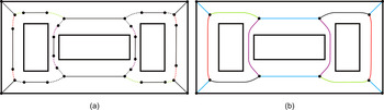
Figure 6 illustrates the impact of the two approaches on the number of branches of the medial axis for a simple planar domain. In this example, by combining the half-spaces bounding each obstacle as described above, we reduce the number of branches of the medial axis from 30 to 14. The number of nodes in the graph will therefore be reduced from 32 to 12.
The half-spaces bounding each individual obstacle are combined so that each obstacle will be defined by one single function, which reduces the number of medial axis branches from 30 to 14. (a) Dashed lines are branches created by intersection of conical half-spaces with the outer half-spaces (see Section 2.2.2). The black dots on the medial axis separate the branches of the medial axis. [A color version of this figure can be viewed online at journals.cambridge.org/aie]

After the medial axis segmentation, the last step in planning a path for a moving point is to perform a graph search algorithm on a weighted graph. Each critical point becomes a vertex in this graph and each branch will be represented as a weighted edge whose weight is proportional to the length of the branch. It should be apparent that the “smaller” the graph the faster the computations. In this work we used the established Dijkstra's algorithm (Dijkstra, Reference Dijkstra1959) that has been widely used in motion planning and routing problems due to its simplicity, efficiency, and robustness. However, one can use any of the other existing graph search algorithms to generate collision-free paths in this weighted graph.
Note that some domains admit more than one shortest path, and that all standard graph search algorithms can be modified to produce all possible shortest paths. The interested reader is referred to Takaoka (Reference Takaoka2005), as well as to standard textbooks on algorithms such as Dasgupta et al. (Reference Dasgupta, Papadimitriou and Vazirani2008).
2.4. A family of skeletons that contains the medial axis
To summarize the discussion above, we are first constructing the distance function over the domain from individual half-spaces defining the boundary of the domain (both outer boundary and obstacles) as described in Section 2.2.2. As a result, we obtain a continuous piecewise smooth surface, whose zero level set is the boundary of the domain. This construction is followed by the extraction of the medial axis as the subset for which the continuous distance function is nondifferentiable.
However, by altering the distance functions defined by each half-space f i ≥ 0, we can deform the medial axis such that the deformed skeleton will be “attracted” or “repulsed” by specific obstacles inside the domain or by specific half-spaces defining the outer boundary of the environment.
In our construction above, we define each halfspace of the original domain as an implicit function f i ≥ 0. Each half-space f i in the d dimensional space  d induces a higher dimensional half-space in
 d+1 denoted by H i ≥ 0.
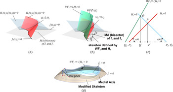
We will describe the concept with the help of a 2-D example, but this discussion naturally extends to 3-D environments. Consider the example shown in Figure 7, which shows two planar half-spaces f 1 and f 2, as well as their exact distance functions that are the boundaries of the corresponding 3-D half-spaces defined by equation H i = 0, namely,


(a) Exact distance functions H 1 = 0 and H 2 = 0 for two planar curves defined by f 1(x, y) = 0 and f 2(x, y) = 0, (b) a weighted distance function WF2 = λ2H 2 = 0 results in a different skeleton than the medial axis, (c) the triangles formed by P i, P′i(i = 1, 2) and the corresponding footpoints flattened on the plane, and (d) a single weight λ is applied on the distance function defining the obstacle f 2 = 0 regardless of how many half-spaces contribute to f 2 = 0. [A color version of this figure can be viewed online at journals.cambridge.org/aie]

Assume that the two surfaces ∂H 1 and ∂H 2 are the exact distance functions to curves f 1 = 0 and f 2 = 0, and that point P is on the intersection curve between ∂H 1 and ∂H 2 as illustrated in Figure 7. By definition, both ∂H 1 and ∂H 1 make with the (x, y) plane an angle of π/4 at the footpoints of P on f 1 and f 2, for all points P ∈ ∂H 1 ∩ ∂H 2. Denote these footpoints by P f 1 and P f 2. Furthermore, assume that λ1 ≥ 0 and λ2 ≥ 0 are two positive real numbers that multiply H 1 and H 2, respectively, such that

Clearly, the functions WF1 and WF2 and are distance functions for curves f 1(x, y) = 0 and f 2(x, y) = 0 if and only if λ1 = λ2 = 1. In this case, by projecting the ridge between WF1 and WF2 onto the plane of f 1 and f 1 we obtain the bisector of f 1 and f 2, that is, the medial axis. However, if we choose λ1 = 1, but we let λ2 > 1 or λ2 < 1, the projection of the ridge will move closer to or farther away from f 2 = 0 as illustrated in Figure 7b. Consequently, the reals λi act as weights and therefore the resulting R-function expression for the domain generates a weighted distance function (denoted here by WF). In fact,

where θi is the angle formed by WFi = 0 and the plane (x, y) at the footpoint P f i on f i = 0 as shown in Figure 7c. The fact that each scalar λi is constrained to be positive definite implies that the angle θi ∈ [0, π/2].
In other words, scalars λi act as degrees of freedom controlling the local attraction or repulsion of the skeleton by f i. Furthermore, because each θi ∈ [0, π/2], the branch of the skeleton defined by two half-spaces f i ≥ 0 and f j ≥ 0 will lie in the region of the plane where both f i > 0 and f j > 0, that is, between f i > 0 and f j > 0.
In this paper, we assign a separate scalar λ to the distance function that defines each obstacle. In other words, each λ will act as a global weight for the corresponding obstacle as shown in Figure 7d. If the function defining each obstacle of the domain, which is represented by one single R-function expression, is weighted by a single weight λ, we conjecture that the resulting skeleton of the domain is homeomorphic to the medial axis, which in turn preserves the homotopy of the domain (Lieutier, Reference Lieutier2003). In this case, the class of skeletons controlled by θi will have the same homotopy as that of the domain.
3. MEDIAL ZONES AS THICK SKELETONS
We have been using the principal system of R-functions given in Eq. (1) with a value of α = 1. This, in turn, generates piecewise smooth distance functions as shown in Figure 3c, and the skeletons are obtained as the nondifferentiable points of the distance function as discussed in Sections 2.5 and 2.6. However, one important feature of R-functions is that they can generate continuous functions over the domain that are differentiable almost everywhere (for a detailed discussion, see Shapiro & Vossler, Reference Shapiro and Vossler1991; Shapiro, Reference Shapiro2007). In fact, this is illustrated in Figure 3 for the principal system of R-functions of Eq. (1), which produces such differentiable functions by simply choosing a value of α < 1.
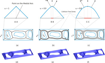
For a given R-function expression corresponding to a given domain we define the medial zones as those points of  d that belong to the surface constructed with R-functions and are “near” the crest of the surface,Footnote 5 as illustrated in Figure 8. The “nearness” can be defined in several different ways and can be computed via Laplacian, Gaussian curvature, or other differential properties of the resulting surface. Note that the differential properties of the resulting surfaces can be controlled by the specific system of R-functions being used. Consequently, by adjusting the value of α and the “nearness” metric, one can “grow” or “shrink” these medial zones. The effect of changing α on the resulting medial zone is illustrated in Figure 8b and c, as detailed in Eftekharian and Ilieş (Reference Eftekharian and Ilieş2010).
Medial zones controlled by the prescribed α values. [A color version of this figure can be viewed online at journals.cambridge.org/aie]

The implications to motion planning are important because these medial zones provide significantly increased flexibility of the resulting path compared to the case in which the paths are planned along the medial axis or skeleton of the same domain. Moreover, these medial zones can be computed with the same computational algorithms as those used to compute the skeletons described above. From a practical point of view, the paths planned based on the medial zones can be shorter and smoother than those planned based on skeletons, which is evident in the examples discussed in Section 4.
4. EXAMPLES
We illustrate the capabilities of our approach with several examples that contain both linear and nonlinear half-spaces in both 2-D and 3-D, as well as moving obstacles that merge with either other obstacles or the boundary of the domain ∂Ω to produce drastic topological changes of the environment. We implemented a commonly used finite-difference approximation of the Laplacian (Bovik, Reference Bovik2005) to extract the ridges and ravines of the weighted distance function.
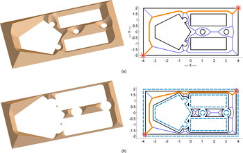
Figure 9a shows the distance function of a domain and the corresponding shortest trajectory of a point between an initial and a final position. By taking a different level set of the distance function, we can plan within the same formulation the path of an object approximated by the smallest enclosing ball as shown in Figure 9b.
(a) The trajectory planning of a point is shown. By taking different level sets of the implicit function induced by the R-function expression, we can plan the path of an object approximated by the (b) smallest enclosing ball. [A color version of this figure can be viewed online at journals.cambridge.org/aie]

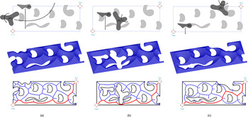
The example in Figure 10 shows three instances during the evolution of an environment in which two obstacles are moving independently while merging and splitting with other obstacles. The planned path adapts to the changing environment as shown in the third row of images in the same figure.
An environment with both static and dynamic obstacles moving independently. The planned path adapts to the changing environment. [A color version of this figure can be viewed online at journals.cambridge.org/aie]

The environment from Figure 10b is illustrated in Figure 11, but with a different path planning goal, namely, to have “sufficient” clearance to the boundary of Ω. The weight λ corresponding to the R-function expression defining the outer boundary of the domain is set to 0.2679 (equivalent to an angle of 15 degrees; see Section 2.6). Note the difference between the resulting shortest path in Figure 11 and that of Figure 10b.
An environment with obstacles similar to the one in Figure 10b. The weight of the outer boundary is λ = 0.2679, which is equivalent to an angle of 15 degrees. [A color version of this figure can be viewed online at journals.cambridge.org/aie]

Figure 12 shows the path planning for a point within a domain with curved boundaries (Fig. 12a) and a second path of an object enclosed by a minimal ball while moving in the same environment. Note that the path planned for the object is different than the path of the point even though the space is the same. This is due to the fact that planning the path of the object is transformed into the path planning of a point by taking a different level set of the R-function expression describing the original environment. In this example the radius of the minimal enclosing ball is 0.3 m.
(a) An environment with curved boundaries and the corresponding trajectory of a point and (b) the problem of planning a path of a moving object is transformed into the path planning of a point by taking a different level set of the distance function corresponding to the original environment. Note the difference in the two planned paths. [A color version of this figure can be viewed online at journals.cambridge.org/aie]

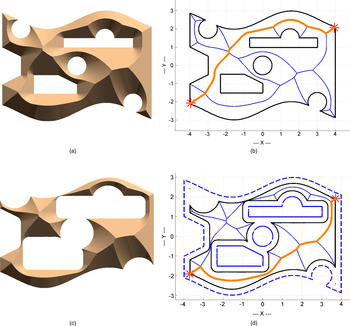
A modified skeleton is shown in Figure 13 along with the computed path of a point within a domain with curved boundaries. The resulting roadmap computed based on the medial axis is shown in Figure 13a. Furthermore, the R-function expression defining the crosshatched rectangular obstacle has been weighted by a factor λ that corresponds to an angle of 85 degrees as discussed in Section 2.6. This effectively brings the skeleton, and therefore the computed path, closer to that particular obstacle. Note that there are five obstacles in this example, some of which are merged together, and that only one of the five corresponding distance functions is weighted. Clearly, other distance functions could be weighted as well depending on the specific path planning task being investigated with important applications in assembly, robotic, or navigation applications (as shown schematically in Fig. 1).
Shortest path of a point within a domain with curved boundaries and five obstacles that was computed based on (a) the medial axis and (b) a skeleton obtained by weighing the distance function defining the rectangular (crosshatched) obstacle. [A color version of this figure can be viewed online at journals.cambridge.org/aie]

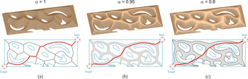
Figure 14 shows a domain containing multiple obstacles with free-form planar geometry. The three different cases illustrated there correspond to three values of α, namely, α = 1, α = 0.95, and α = 0.8, which result in the illustrated distance functions. For the case when α = 1 illustrated Figure 14a the resulting skeleton is the medial axis, and the resulting shortest path is shown in orange (lighter color). By decreasing the value of α we increase the smoothness of the distance function, which in turn increases the “thickness” of the medial zones, which is illustrated in Figures 14b and c. Note that as α increases the length of the roadmap decreases, while its smoothness increases.
Shortest paths of a domain containing multiple obstacles with free-form planar geometry. The paths have been computed based on medial zones for three values of α. [A color version of this figure can be viewed online at journals.cambridge.org/aie]

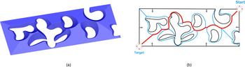
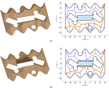
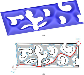
The R-function expression describing the domain of Figure 10b is illustrated in Figure 15a with a value of α = 0.90, which results in the medial zone shown in Figure 15b. Observe that this new distance function effectively results in a smoother shortest path (Fig. 15b) that takes a different route than the shortest path shown in Figure 1b for the same domain.
Medial zone and shortest path for the domain of Figure 1b for a value of α = 0.9. The path computed in (b) is shown with dotted line for comparison purposes. [A color version of this figure can be viewed online at journals.cambridge.org/aie]

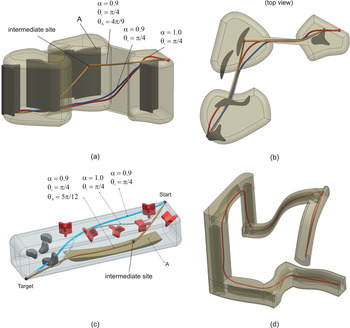
Finally, Figure 16 shows several 3-D examples and the corresponding shortest paths. The 3-D domains shown in Figure 16a and b contain one intermediate site that must be part of the path that is being planned. Note that a path along the medial axis that would satisfy these constraints does not exist. These examples contain two paths that do not satisfy the intermediate site constraint, which are planned inside two medial zones corresponding to values of α = 1 and α = 0.9, respectively. The same examples show a third path, which, in each case, is the shortest path connecting the beginning and end configurations, passing through the intermediate site, while remaining inside a medial zone corresponding to a value of α = 0.9. To achieve this, the distance function corresponding to the proximate obstacle (A) was modified in both examples as described in Section 2.6 and obstacle A “attracts” the resulting path. The example shown in Figures 16d illustrates another path planning scenario in an environment that contains many narrow passages and freeform obstacles.
Collision-free paths for several 3-D domains computed based on medial zones. The intermediate sites in (a) and (c) are shown as a points: the three paths correspond to values of α = 1 and α = 0.9; (b) the top view of the environment from (a); and (d) an environment with narrow passages. [A color version of this figure can be viewed online at journals.cambridge.org/aie]

5. CONCLUSION
This paper formulates a family of geometric skeletons that contains the medial axis as a special case, and explores their use in robotic path planning applications in highly dynamic and topologically evolving environments. We propose a strategy for constructing these skeletons that relies on constructive representations of shapes with R-functions that operate on real-valued half-spaces as logic operations. The flexibility provided by the underlying Boolean nature of the proposed framework makes this approach well suited to problems involving substantial geometric and topologic changes of the environment. Note that our approach
1. is applicable for general closed, bounded, regular, and semianalytic domains;
2. results in a family of skeletons that contains the medial axis as a special case. The computed skeleton can be modified so that the computed path is attracted or repulsed by prescribed obstacles within the domain;
3. can compute the medial zones that intuitively represent thick skeletons of the domain. One important advantage of these zones in the context of motion planning applications is that they generate shorter and smoother paths than medial-axis path planning strategies for the same environment;
4. can handle problems with evolving environments or in which the environment is not fully known a priori because obstacles can be introduced/removed at any time during the planning stage and within the same problem formulation;
5. intrinsically supports local and parallel skeleton computations for domains with rigid or evolving boundaries due to the explicit mapping between the branches of the medial axis and the half-spaces bounding the environment;
6. can handle trajectory planning of points as well as path planning for 2-D/3-D objects within the same formulation due to the close relationship between R-function expressions and level sets. The simplest approach to extend the trajectory planning to solid objects is to approximate the moving object by its smallest enclosing ball, and take different level sets of the distance function defining the environment. This effectively offsets the boundary of the environment so that the outer boundaries of the environment shrink while, at the same time, the obstacles grow by the same radius of the disk enclosing the object; and
7. supports multiple representations of the input geometry;
We argue in this paper that the degrees of freedom that we used to control the subset of the domain in which we are looking for the shortest path afford significant flexibility in computing paths that satisfies specific geometric constraints that are common in geometric reasoning and motion planning applications. In addition, the attractive and repulsive factors λi provide a simple and elegant mechanism to deform the skeleton so that the resulting path gets closer to or farther away from specific sites or obstacles in the environment.
We conjectured that the family of skeletons defined by weights λ as defined in Section 2.4 is homeomorphic to the medial axis, which implies that the skeletons in the family are homotopic to the domain. This property coupled with the fact that the family of skeletons is really defined by pseudodistance functions is crucial in all potential applications such as unmanned vehicles navigation systems, robotics, autonomous assembly systems, and shape representation and recognition.
ACKNOWLEDGMENTS
This work was supported in part by National Science Foundation Grant CMMI-0555937 and CAREER Awards CMMI-0644769, CMMI-0856401, and CNS-0927105.
Ata Eftekharian is a Postdoctoral Fellow in the Automated Design Lab, Department of Mechanical Engineering, at the University of Texas at Austin. Dr. Eftekharian has MS and PhD degrees in mechanical engineering from Sharif University of Technology and University of Connecticut, respectively. His research interests include geometric modeling, computer-aided design and manufacturing systems, and artificial intelligence. His research work mainly focuses on developing new theories and techniques for automating synthesis of mechanical artifacts, path planning, and topics related to reasoning about manufacturability and design changes.
Horea Ilieş is an Associate Professor of mechanical engineering and computer sciences at the University of Connecticut, where he established the Computational Design Laboratory. Prior to that, he spent several years with Ford Motor Company in research, manufacturing, and product design and development. His current research interests include geometric and physical computing, shape synthesis and geometric reasoning, as well as biomolecular engineering. Horea received the NSF CAREER award in 2007.
 d+1 space.