Identification

We propose a new identification strategy that allows testing whether central bank balance sheets played the roles described earlier. In the context of the classical gold standard, a change in the discount rate of the BoE provides an exogenous shock that affects international capital flows in all countries in the same way. A change to the discount rate of the BoE—the conductor of the orchestra in Keynes’ famous words, an assessment supported by subsequent research (Lindert Reference Lindert1969; Eichengreen Reference Eichengreen1987; Morys Reference Morys2013; Bazot, Bordo, and Monnet Reference Bazot, Bordo and Monnet2016)—is the quintessential shock to the exchange rate of another country. An increase in the BoE discount rate would attract capital to England and create capital outflows and exchange rate depreciation elsewhere.

The advantage of such an identification is twofold. First, movements in the BoE discount rate can be deemed exogenous to the behavior of other central banks during this period (see our discussion later). This assumption is also the basis for the work of Obstfeld and Taylor (Reference Obstfeld and Taylor2004) and Jordà et al. (2019) on the trilemma during the gold standard period. Second, we can verify—for each country—whether this shock is indeed a shock that is likely to drive capital flows by looking at the reaction of the exchange rate.

This identification is consistent with the recent literature looking at today’s influence of U.S. interest rates on the global financial cycle (starting with the seminal study of Rey (Reference Rey2016)). We will show in the robustness section that our conclusions still hold if we use alternative measures of exogenous English monetary policy shocks.

Theoretical Predictions

The trilemma in international macroeconomics implies the following four scenarios after an increase in the BoE discount rate: The first scenario is equivalent to the plain trilemma case with a fixed-exchange rate and full capital mobility. It would also be equivalent to the “rules of the game” as defined in the gold standard literature. Scenario 2 is the same case where we consider the role of the central bank’s domestic and international assets in rounding the corners of the trilemma, as explained in the previous section. This scenario is usually not investigated in empirical studies of the trilemma, as it requires balance sheet data. Scenario 3 is the trilemma case with fixed-exchange rates and capital controls. Scenario 4 is the case with floating exchange rates.

Method of Estimation

We study the reaction of central banks’ balance sheets, exchange rates, and interest rates to an exogenous increase in the BoE rate. Our identification strategy allows us to study simultaneously the degree of monetary autonomy (the response of the domestic rate to the English rate) and the means employed by central banks to achieve such autonomy (domestic loans, foreign exchange interventions, floating exchange rates, or imperfect convertibility).

Following a now well-established empirical literature on the effects of monetary policy shocks (Jordà Reference Jordà2005; Ramey Reference Ramey, John and Uhlig2016; Jordà et al. 2019), we use local projections to estimate the effect of a shock on the BoE interest rate. This method allows estimating impulse-responses (IR) directly from an exogenous shock without relying on a predefined model.

Let K be the dimension of the vector of macroeconomic aggregates of interest. M is the number of countries, T is the time dimension, and H is the time horizon for which we want to measure the response to a shock. Let $y_{i,t + h}^k$ be the value of variable k = 1, …, K observed for a country i = 1, …, M, for which we measure the response to a shock on the BoE rate in horizon 0 ≤ h ≤ H. Lastly, let Y _i,t denote the vector of $y_{i,t}^k$ variables.

If $$r_t^{BoE}$$ is the BoE discount rate, the impulse response to a shock (δ) on $$r_t^{BoE}$$ is measured as:

$$IR\left( {y_{i,t + h}^k,\delta } \right) = {E_{it}}\left( {y_{i,t + h}^k|\delta = 1;{Y_{i,t}},{Y_{i,t - 1}}, \ldots } \right) - {E_{it}}\left( {y_{i,t + h}^k|\delta = 0;{Y_{i,t}},{Y_{i,t - 1}}, \ldots } \right)$$

.

A shock δ = 1 means that $$r_t^{BoE}$$ increases by 100 basis points.

The local projections consist of measuring $$IR\left( {y_{i,t + h}^k,\delta } \right)$$ based on a sequence of predictive fixed effects panel regressions of the variable of interest on an exogenous shock to horizon h:

$$y_{(i,t + h)}^k = {\alpha _i} + {\Phi _h}(L){Y_{(t - 1)}} + {\beta _h}\Delta r_t^{BoE} + trend + {\varepsilon _{h,it}}for\,h = 0,1,2, \ldots ,H,$$

where Φ _h (L) is the polynomial set of lag operator (which is set at 3 in our analysis), the unanticipated change in the BoE discount rate, α _i the country fixed effects, and ε _h,it the residual. The IR is the set of estimated $$\widehat {{\beta _h}}$$ from h = 0 to h = H.Footnote ⁴ There are as many sequences as there are variables of interest. Following Ramey (Reference Ramey, John and Uhlig2016), we include a trend in the estimation to account for potential non-stationarity (none of our results are sensitive to this assumption).

Starting with h = 0 rather than h = 1 is a timing restriction, implying that domestic macroeconomic variables can respond immediately to a change in the interest rate of the BoE.Footnote ⁵ In practice, central banks moved their own discount rates, typically a few days after the BoE changed its rate (for a similar observation, cf. Lindert (Reference Lindert1969)).

Sources

Our dataset is based on an exceptional source that has never been exploited before.Footnote ⁶ The French central bank (Bank of France) began collecting systematically the weekly or monthly balance sheets of all central banks worldwide in 1891. Central banks publish these balance sheets at a high frequency, in addition to their annual reports to shareholders. The legal (or in some cases, customary) obligation to publish these balance sheets was justified by the requirements to which central banks were subject in terms of the relationship between the currency in circulation and the reserves, or the ceilings on circulation. Figures of banknotes in circulation and gold reserves were carefully looked at by policymakers and investors; they were published in major financial newspapers, alongside data on exchange rates and discount rates (e.g., L’Economiste Européen in France, The Banker in the United Kingdom, Le Moniteur in Belgium, see Baubeau (Reference Baubeau2018)). However, newspapers did not publish data on other central bank assets, which were far more difficult to harmonize and compare, given the different accounting practices of countries.Footnote ⁷

The Bank of France took on this difficult and tedious task. Sufficient skills were needed to translate and understand the various reports. We use monthly data to achieve the highest possible frequency available for all central banks.Footnote ⁸ We also consulted the annual balance sheets, likewise prepared by the Bank of France and based on the annual reports of the respective central banks, in order to establish whether some balance sheet items were missing from the weekly and monthly publications.Footnote ⁹ For instance, in a limited number of cases and only when numbers were small, foreign exchange reserves were only published in the annual report (see Online Appendix).

Data

The joint evolution of domestic and international portfolios is key to our analysis. Fortunately, the harmonized balance sheet provided by the source helped build those series. For each country, we assembled five major series: (1) metallic reserves (gold plus silver); (2) foreign paper (bills of exchange drawn on foreign places); (3) funds held abroad; (4) discount portfolio of domestic paper; (5) short term advances on securities and other collateral. (1), (2), and (3) constitute the international portfolio, while (4) and (5) capture the domestic portfolio. Details about all five series are available in the Online Appendix.

Our dataset includes 21 central banks, encompassing all central banks worldwide during the period 1891–1913 (the Swiss National Bank was created only in 1908 and the U.S. Federal Reserve in 1913). As Italy had three large banks of note issue (Bank of Italy, Bank of Naples, and Bank of Sicily), we have a panel data set of 19 countries with a central bank.Footnote ¹⁰ The Online Appendix discusses a few other cases of multiple banks of issue. In the next section, we will add one country without a central bank (the United States) for the purpose of comparison.

Series of discount rates of these central banks are also available in our original source (and compiled in Roulleau (Reference Roulleau1914)), which we double-checked with the daily discount rate data underlying Morys (Reference Morys2013) for 12 of the countries in our study. For two reasons, we use official discount rates and not private discount rates. First, we are interested in the constraints imposed upon the central banks: how did their main policy instrument need to change in response to a discount rate increase by the BoE? Second, while we are aware that international arbitrage was at the heart of the adjustment mechanism described in this paper, and that arbitrageurs were motivated by private rather than official rates, we simply do not have data on private rates for enough countries; or, to be more precise, in the majority of countries in which money market rates are published by the Economist, they are simply equal to the central bank policy rate (Neal and Weidenmier Reference Neal, Weidenmier, Michael, Alan and Jeffrey2003).Footnote ¹¹ This implies that using the published market rates for peripheral countries is equivalent to using the central bank discount rate (as done by Mitchener and Weidenmier (Reference Mitchener and Weidenmier2015) to compute risk premia over this period). We ran robustness checks for all countries for which we could muster private discount rate data (France, Germany, the Netherlands, Austria, and Belgium), with results qualitatively no different from our baseline estimations (Online Appendix Figure A-8). Our only half-successful attempt to collect private rates has shown us that domestic money markets remain insufficiently understood. This is the case even for core countries like Germany (Morys Reference Morys2021b). Based on our knowledge of the South-East European economies, we do not think that the equivalence between money market rates and central bank rates in most countries implied that there was no money market. It only means that there was no centralized market price, but interbank peer-to-peer lending and similar activities almost certainly took place (transactions for which the central bank rate served as a reference point). This view is supported by ample evidence that the foundation of banks of note issue in peripheral countries was typically motivated by lowering (and to some extent regulating) pre-existing money market rates (Morys Reference Morys2014). Moreover, even in countries like France, with a well-established money market for prime bills between a small number of banks (Bazot, Bordo, and Monnet Reference Bazot, Bordo and Monnet2016), the discount of commercial paper was typically conducted at the central bank rate throughout the country (Roulleau Reference Roulleau1914, pp. 159–62).

Finally, we gathered a monthly series of exchange rates for London from various sources, mostly from Schneider, Schwarzer, and Zellfelder (Reference Schneider, Schwarzer and Zellfelder1991, Reference Schneider, Schwarzer and Zellfelder1994, Reference Schneider, Schwarzer and Zellfelder1999) and Morys (Reference Morys2013).Footnote ¹² We use exchange rates as a deviation from mint parity (that is the official exchange rate between gold and domestic currency). Mint parities were also available in our original source, in the archives of the Bank of France. Countries off the gold standard also have a mint parity, but central banks in these countries had no commitment to redeem notes in gold at such a price. For reasons of consistency, all data (balance sheet data, discount rates, and exchange rates) are end-of-the-month values. For all countries except Japan, the monthly balance sheet of the central bank is available starting in the early 1890s; usually as soon as January 1891. Data on Japan start in 1899, one year after the country entered the gold standard. For a significant number of countries, we have data on their central banks both before and after they joined the gold standard.

Groups of Countries

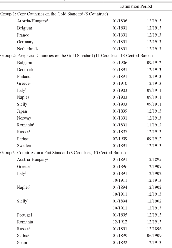
There is no reason to believe that the 21 central banks in our sample behave in the same way, particularly because they did not all have the same exchange rate regime and level of financial integration. For this reason, we will look at different groups of countries—defined in a way that is consistent with the historical context and the literature on the gold standard—and we will discuss how close they were to the theoretical predictions of Section 2. We distinguish three groups of countries with a central bank: (1) core countries on the gold standard; (2) peripheral countries on the gold standard; and (3) countries with a floating exchange rate (fiat standard).

As for gold standard adherence, we follow the consensual classification that has emerged from an extensive literature on this matter (Flandreau and Zumer Reference Flandreau and Zumer2004; Obstfeld, Shambaugh, and Taylor Reference Obstfeld, Shambaugh and Taylor2005; Mitchener and Weidenmier Reference Mitchener and Weidenmier2015; Morys Reference Morys, Pfister, Hesse, Spörer and Wolf2021a).Footnote ¹³ The distinction between groups (1) and (2) hinges upon the definition of core versus periphery. Economic historians agree to consider Belgium, England, France, Germany, and the Netherlands as core countries in the international financial system because they had mature money markets, a liquid foreign exchange market, and could issue sovereign debt in their own currency (Bordo and Flandreau Reference Bordo, Flandreau, Michael, Alan and Jeffrey2003, p. 349; Flandreau and Jobst Reference Flandreau and Jobst2005; Morys Reference Morys2013). Outside this group, Austria-Hungary is a borderline case. Money and exchange markets were liquid and well-developed (Reichsbank 1925, pp. 212–31; Jobst Reference Jobst2009), but Austria-Hungary had to insert gold clauses into their bonds to issue them abroad (Morys Reference Morys2006). Since sovereign debt is less crucial to our study, we decided to classify Austria-Hungary as a core country. Such an approach is vindicated by a statistical analysis of Austria-Hungary on its own, when its results are in line with all other core countries. The empirical conclusions presented in the next section are not qualitatively modified if Austria-Hungary is included in the periphery.

Table 1 summarizes our three groups of countries, with details about a country’s date of entry into and exit from the gold standard (“estimation period”) where relevant. When a country joins the gold standard, it moves from Group 3 to Group 1 or 2. Therefore, a country may appear in two groups but with different estimation periods.

Table 1

Country groups: Core countries on gold, peripheral countries on gold, fiat standard countries

Notes: ¹ Also in group 3 for other estimation periods. ² Also in group 1 for other estimation periods. ³ Also in group 2 for other estimation periods.

Sources: Gold standard adherence based on de-facto exchange-rate classification proposed by Obstfeld, Shambaugh, and Taylor (Reference Obstfeld, Shambaugh and Taylor2005) and exchange-rate sources as described in the main text.

Specification and Variables

Local projections are easy to estimate with state-dependent variables. We can thus include “gold standard” and “core-periphery” dummy variables to interact with the set of other variables. This allows us to estimate the effect of the shock for each group of countries defined in the previous section. As such, we use three different models (one for each group):

$$\eqalign{ & y_{i,t + h}^k = {\alpha _i} + core\,in\,G{S_{t - 1}} \times \left[ {{\Phi _h}\left( L \right){Y_{t - 1}} + {\beta _{a,h}}\Delta r_t^{BoE}} \right] + trend + {\varepsilon _{h,it}} \cr & y_{i,t + h}^k = {\alpha _i} + periphery\,in\,G{S_{t - 1}} \times \left[ {{\Phi _h}\left( L \right){Y_{t - 1}} + {\beta _{b,h}}\Delta r_t^{BoE}} \right] + trend + {\varepsilon _{h,it}} \cr & y_{i,t + h}^k = {\alpha _i} + floatin{g_{t - 1}} \times \left[ {{\Phi _h}\left( L \right){Y_{t - 1}} + {\beta _{c,h}}\Delta r_t^{BoE}} \right] + trend + {\varepsilon _{h,it}} \cr} $$

core in GS is a dummy variable equal to 1 if the country belongs to the core and adheres to the Gold Standard at time t, periphery in GS is a dummy variable equal to 1 if the country belongs to the periphery and adheres to the Gold Standard at time t, floating is a dummy variable equal to 1 if the country’s exchange rate is floating. β _a,h , β _b,h , and β _c,h , are picked up from h = 0 to h = H, to build impulse response functions (IRFs) for each group. Thus, β _a,h corresponds to the response of group 1, β _b,h corresponds to the response of group 2, and β _c,h corresponds to the response of group 3.Footnote ¹⁴

The variables of interest included in our benchmark estimations are the following: the BoE discount rate (in percent); the natural logarithm of total international assets; the natural logarithm of total domestic assets; the country-specific central bank discount rate; and the exchange-rate deviation from mint parity (with positive values denoting depreciation). The vector of control variables is composed of three lags for each variable of interest. Panel data unit root tests have been performed based on Fisher-type tests and Im-Pesaran-Shin tests. Non-stationarity is rejected in all cases at the 1 percent confidence interval. Each regression includes country-fixed effects. To correct for heteroskedasticity and serial correlation, we use clustered standard errors when estimation is in a panel, or use the Newey West procedure when the estimation is for a single country (the United States, in the next section).

In the figures, we look at the responses of the following variables to an increase in the discount rate of the BoE by 1 percent (100 basis points). We report two standard-error bands for impulse responses. Given the aforementioned data manipulations, responses are read in all four cases as the percentage change compared to month t = –1 (with positive values in the lower right panel meaning depreciation).Footnote ¹⁵

Core Countries

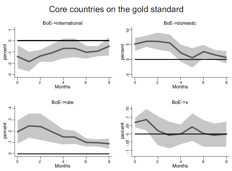
Figure 1 shows how core countries reacted to a shock in the BoE discount rate. They increased their interest rate only by a small magnitude: 24 basis points after a shock of 100 basis points. Put differently, the interest rate pass-through is much lower than unity and amounts to approximately 24 percent (for a similar finding from a different estimation perspective Obstfeld and Taylor (Reference Obstfeld and Taylor2004) and Morys (Reference Morys2013)). This imperfect pass-through allows for arbitrage in international markets. The exchange-rate depreciation is rather small (+0.08 percent, with positive values denominating depreciation), and comes back to parity after two months. This result contrasts with peripheral countries where depreciation was greater and of longer duration (see Figure 2).

Figure 1

THE REACTION OF CENTRAL BANKS IN GOLD STANDARD CORE COUNTRIES TO AN ENGLISH DISCOUNT RATE SHOCK OF 100 BASIS POINTS IN THE FIRST EIGHT MONTHS

Units: Percentage change compared to month t = –1 (positive exchange-rate response in lower right panel indicates depreciation).

Notes: “international” and “domestic” denote the international and domestic portfolios of central banks, “rate” is the discount rate of central banks, and “x” the exchange rate on London. Sources: Own calculations based on sources as described in the main text and the Online Appendix.

Figure 2

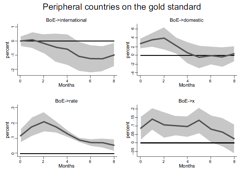
THE REACTION OF CENTRAL BANKS IN GOLD STANDARD PERIPHERAL COUNTRIES TO AN ENGLISH DISCOUNT RATE SHOCK OF 100 BASIS POINTS IN THE FIRST EIGHT MONTHS

Units: Percentage change compared to month t = –1 (positive exchange-rate response in lower right panel indicates depreciation).

Notes: “international” and “domestic” denote the international and domestic portfolios of central banks, “rate” is the discount rate of central banks, and “x” the exchange rate on London.

Sources: Own calculations based on sources as described in the main text and the Online Appendix.

What were the balance sheet effects? As core countries offered (almost) unconditional and unlimited convertibility, the international portfolio declines quickly and substantially: 1.8 percent after one month.Footnote ¹⁶ Yet core countries dilute the impact of this reserve drain by expanding domestic credit. The reaction of the domestic portfolio is, in percentage terms, more than three times larger than the reaction of the international portfolio, namely 5.5 percent after one month. As the international portfolio was on average twice as large as the domestic portfolio, it was thus necessary to increase the domestic portfolio in absolute numbers by more than the decline of the international portfolio.

Adjustment operates quickly, with the exchange rate and central banks’ balance sheet responses becoming statistically insignificant after three to four months. This short-term adjustment is consistent with the high level of financial integration that characterized the gold standard era. It also means that we would not be able to capture adequately the role of central banks as shock absorbers if we worked with quarterly or annual data.

Our results can contribute to the debate on foreign exchange intervention, if we separate the series “international portfolio” into its components, namely “metallic reserves” (time series 1) and “foreign exchange” (time series 2 and 3, i.e., “foreign paper” plus “foreign funds”). In line with the literature that has studied such interventions in core countries (see in particular Jobst (Reference Jobst2009) on Austria and Ugolini (2012) on Belgium), we observe a very strong response of foreign exchange assets. For the three out of five core countries for which we have monthly data on foreign exchange for the entire period (Belgium, Austria, and the Netherlands), Figures A1a, A1b, and A1c (reproduced in the Online Appendix) document the systematic use of foreign exchange interventions. We also find that the response of the “metallic reserves” (gold stock) is still negative and significant (except in the case of Belgium), but that the response of foreign exchange assets is far larger. As results are expressed in percentage change, a stronger response of foreign exchange is partly explained by the fact that the gold stock was larger than the stock of foreign exchange reserves in these central banks (83 percent of the total international portfolio on average). The absence of gold outflows in Belgium is consistent with the fact that foreign exchange assets constituted a much larger share of total international assets in this country (about half) and the National Bank of Belgium was able to rely on liquid and well-developed local markets so that it could actually deploy sophisticated foreign exchange interventions.

The Gold Standard Periphery: Imperfect Convertibility

Countries on the gold standard periphery react fundamentally differently to core countries along all four dimensions (Figure 2), yet the most striking difference relates to the absence of immediate reaction in the international portfolio in the periphery. For the first four months, results are not statistically different from zero at the 5 percent level. This quantitative finding confirms the qualitative statement of Martín-Aceña, Martínez-Ruiz, and Nogues-Marco (Reference Martín-Aceña, Martínez-Ruiz, Nogues-Marco, Ögren and Øksendal2012) on the absence of gold convertibility on the periphery, which—to the best of our knowledge—has never been assessed econometrically. Distinguishing in the international portfolio between foreign exchange and gold does not change the results. The responses of both types of assets are not significant (Figure A-2 in the Online Appendix).Footnote ¹⁷

This is accompanied by a sharper and longer reaction in the exchange rate. The exchange rate on the periphery depreciates not only by 70 percent more than in core countries, but it does not bounce back after month one. It remains at depreciated levels for several months instead. Imperfect convertibility allows peripheral countries to let the exchange rate depreciate more strongly than under the scenario of perfect convertibility between gold and domestic currency. Core countries could not afford such a depreciation, as gold points were narrow between Europe’s financial centers and their commitment to convertibility beyond doubt.Footnote ¹⁸

The response of the interest rate and the domestic portfolio reveals differences and similarities to core countries. As in the core countries, the discount rate reacts significantly to the English shock, but smaller (0.17 percent after one month, compared to 0.24 percent for the core) and in a protracted fashion (as opposed to an immediate re-bounce for the core countries). Second, the central bank’s domestic portfolio increased, although there was no loss of foreign reserves in the central bank. Therefore, after an increase in international interest rates, the national central bank had to extend credit to the domestic economy in response to the commercial banks’ demand at its discount window (Bloomfield Reference Bloomfield1959; Bazot, Bordo, and Monnet Reference Bazot, Bordo and Monnet2016). This finding means that there was still a transmission of the English interest rate increase to the domestic money market in the periphery, so that it became cheaper to borrow from the central bank than from the private market. Restrictions on gold convertibility could protect the central bank’s cover ratio (ratio of reserves to banknotes) and widen the exchange rate range, but they were not sufficient to completely isolate the country from international financial markets (as shown by the fact that the exchange rate fluctuates). An increase in domestic loans was still necessary to maintain the domestic interest rate stable, but of a lower order of magnitude than in the core countries.

In sum, peripheral countries were able to shelter from the global cycle by potentially imposing capital controls. This deviation from a central pillar of the gold standard made their adherence less credible (Mitchener and Weidenmier Reference Mitchener and Weidenmier2015)—or, vice versa, low credibility forced them to impose restrictions on gold convertibility—but it did allow them to combine quasi-fixed-exchange rates (albeit with larger bands) with a certain level of monetary policy autonomy.

Incidentally, comparisons between all four core vs. periphery responses help explain why peripheral gold standard countries limited convertibility. Core countries raise their discount rates fast and sizeably (although much less than the BoE), bringing in foreign funds quickly given high levels of financial integration between Europe’s main financial centers. Adjustment was further helped by private agents who deemed the core countries’ adherence to gold credible and bought domestic currency when it was “cheap”, that is, depreciated within the gold points (Bordo and MacDonald Reference Bordo and MacDonald2005). By contrast, lower levels of financial integration and reduced credibility meant that the discount rate was a less sharp weapon for peripheral countries. This, in turn, created a reliance on—partial or complete—inconvertibility to make the gold standard work in this set of countries. Practice differed between countries (see Bloomfield (Reference Bloomfield1959) and Ford (Reference Ford, Mathias and Pollard1989) for a review of gold devices), but immediate and unlimited convertibility remained a characteristic of the peripheral countries until the end of the classical Gold Standard period (Martín-Aceña, Martínez-Ruiz, and Nogues-Marco Reference Martín-Aceña, Martínez-Ruiz, Nogues-Marco, Ögren and Øksendal2012; Morys Reference Morys2013, Reference Morys2014, Reference Morys2017).

It might well be that the benevolent combination documented here was more readily available in the post-1890 environment of a mildly inflationary gold standard (as opposed to the deflationary pressures of the 1870s and 1880s), which coincides with our dataset. Such a view is consistent with the observation that only then do we see large numbers of peripheral countries joining gold. Be this as it may, for the quarter century analyzed here peripheral countries found an institutional adaptation of the gold standard that suited their needs and enabled the countries to make the external constraint more bearable to them (in the same vein Morys (Reference Morys2013)).

Floating Exchange Rates

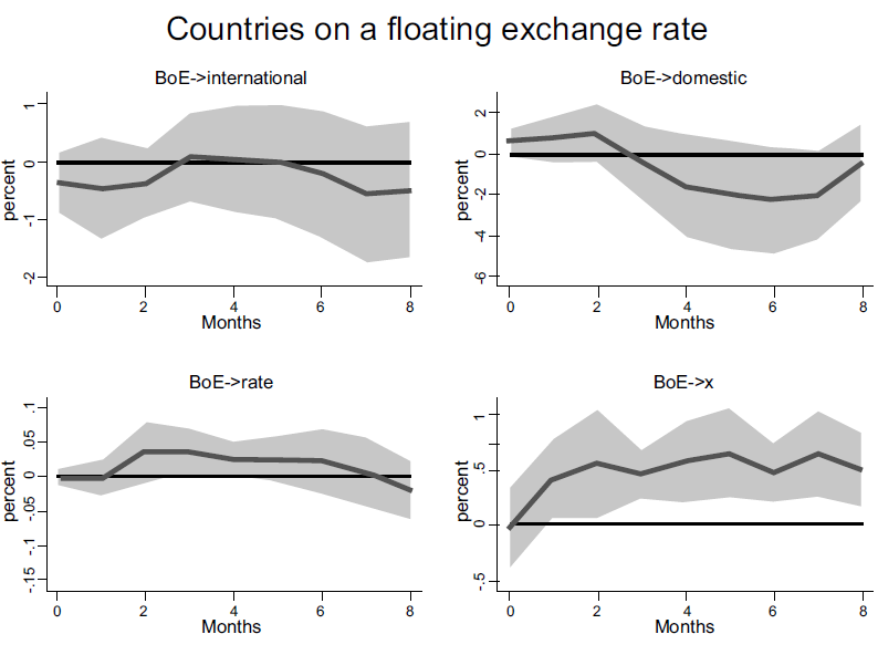
In line with the predictions of the trilemma (Obstfeld and Taylor Reference Obstfeld and Taylor2004), countries that are not on gold simply float their exchange rate in response to an international shock, as shown in Figure 3. Only the exchange rate response is statistically significant, but this particular variable reacts more strongly by a wide margin than in gold standard countries. It falls 0.45 percent in month one, which is approximately five times as much as in core countries and three times as much as in peripheral countries on gold; and the exchange rate remains at depreciated levels thereafter. In floating countries, the burden of adjustment is borne entirely by the exchange rate, so that the central bank exhibits no statistically significant reaction either in its discount rate or on its balance sheet.Footnote ¹⁹

Figure 3

THE REACTION OF CENTRAL BANKS IN FIAT STANDARD COUNTRIES TO AN ENGLISH DISCOUNT RATE SHOCK OF 100 BASIS POINTS IN THE FIRST EIGHT MONTHS

Units: Percentage change compared to month t = –1 (positive exchange-rate response in lower right panel indicates depreciation).

Notes: “international” and “domestic” denote the international and domestic portfolios of central banks, “rate” is the discount rate of central banks, and “x” the exchange rate on London.

Sources: Own calculations based on sources as described in the main text and the Online Appendix.

The United States of America

The most important country without a central bank during this period was the United States. It was on the gold standard, although this system was more contested than in most other countries, and political support for bimetallism remained strong until the 1896 U.S. presidential election. A large number of studies have examined what could have happened to the U.S. economy if a central bank had existed before 1913. There is consensus that a central bank would have smoothed seasonal fluctuations in credit and interest rates (Mankiw and Miron 1986) and perhaps reduced the frequency of banking crises (Davis, Hanes, and Rhode Reference Davis, Hanes and Rhode2009; Hanes and Rhode Reference Hanes and Rhode2013; Bordo and Wheelock Reference Bordo, Wheelock, Michael and Roberds2011). However, precise comparisons with central bank operations over the same period remained limited due to the lack of data.

A simple extension of our previous analysis is to compare the reaction of the U.S. economy to that of countries with a central bank. The United States had no central bank, so the Treasury was responsible for backing banknotes in circulation with gold.Footnote ²⁰ A more difficult choice relates to what constitutes a “domestic portfolio.” On some level, there simply was no domestic portfolio, as there was no U.S. institution with a discount portfolio and short-term advances on securities. Excluding this variable altogether might be the most straightforward implementation of the idea of comparing the United States to countries with a central bank.

Yet, while the United States did not have a European-style domestic portfolio, we cannot conclude from this that the Treasury did not perform some proto-central bank functions.Footnote ²¹ To illustrate this point, the Treasury placed some of its funds on deposit with commercial banks, increasing them in times of monetary stringency and decreasing them subsequently (Friedman and Schwartz Reference Friedman and Schwartz1963, pp. 149–52). Such activities of the Treasury became a more regular feature after the turn of the century, with some contemporaries wondering whether the Treasury might one day act as a central bank (a discussion cut short by the 1907 American Banking Crisis, which eventually paved the way for the establishment of the Federal Reserve System in 1913).

We steer a middle ground. In our baseline estimations, we use the time series for deposits of the U.S. Treasury in national banks as a domestic portfolio,Footnote ²² while noting that this time series is of much smaller magnitude than the domestic portfolio in all other cases. For the United States, the ratio relative to the international assets was 33 percent, while it was 92 percent for gold standard countries with a central bank.Footnote ²³ The size alone raises serious doubt as to the Treasury’s capacity to act as a central bank. Yet, including the data are the only way of answering this important question. We perform the U.S. estimations without a domestic portfolio altogether as a robustness check and reproduce them in the Online Appendix (Figure A-4). Results remain unchanged qualitatively.

Another delicate choice concerns the relevant U.S. market interest rate that we should compare with counterparts in countries with a central bank, namely commercial paper (baseline results) vs. call money (Online Appendix). As already discussed by contemporaries (Roulleau Reference Roulleau1914, pp. 159–62), the most appropriate rate to compare with European discount rates is the interest rate on 60–90 day commercial paper in New York. We collected end-of-the-month values of this rate from the Commercial and Financial Chronicle.Footnote ²⁴

Alternatively, we perform the same analysis using the call money rate in New York (Online Appendix Figures A5, A6, and A7), since several authors argue that it relates to a wider market and is more representative of U.S. financial conditions (Hanes and Rhode Reference Hanes and Rhode2013).Footnote ²⁵ This money market rate was not an interbank rate, but the rate of overnight loans from banks to stock market brokers.

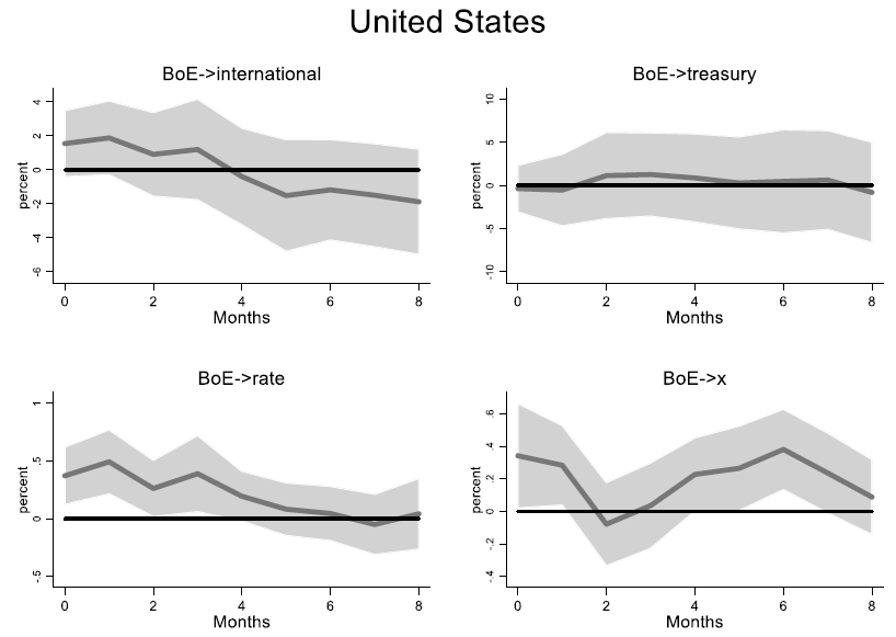
Figure 4 presents the results of local projections with U.S. data, from January 1891 to December 1913. The only variable reacting in a statistically significant way is the interest rate. Note that the interest-rate pass-through is much higher than in gold standard countries with a central bank: approximately twice as high as in core countries (0.49 percent after one month compared to 0.24 percent) and thrice as high as in peripheral countries (0.49 percent compared to 0.17 percent). Put differently, the United States is closest to scenario 1 outlined previously (playing by the rules of the game), as a sizeable domestic portfolio—a key adjustment factor for gold standard countries with a central bank—cannot come to the rescue in the absence of a central bank. In countries with a central bank, the central bank discount rate was an upper limit for the money market rate, since banks could always borrow from the central bank if it was cheaper. In the absence of such an upper limit, the U.S. money market rate was much more responsive to international shocks.Footnote ²⁶

Figure 4

THE REACTION OF THE U.S. MONETARY SYSTEM TO AN ENGLISH DISCOUNT RATE SHOCK OF 100 BASIS POINTS IN THE FIRST EIGHT MONTHS

Units: Percentage change compared to month t = –1 (positive exchange-rate response in lower right panel indicates depreciation).

Notes: “international” denotes the gold reserves of the U.S. Treasury, “rate” is the commercial paper rate in New York, and “x” the exchange rate in New York on London.

Sources: Own calculations based on sources as described in the main text and the Online Appendix.

A direct comparison of the response of the Treasury deposits at national banks with the response of the domestic portfolios of all other gold standard countries is instructive. Figures 1 and 2 show statistically significant responses of the domestic portfolio, larger in absolute number than the outflows of gold and foreign exchange. By contrast, there was no systematic pattern to the Treasury response, hence the statistically insignificant response. Whatever the Treasury might have done exactly, it did not provide the “sheltering” function assigned to the central bank by Polanyi in the quotation given at the beginning of this paper. Before the establishment of the Federal Reserve System in 1913, the U.S. monetary system lacked such a “cushion” (Polanyi) and in turn relied more strongly on the interest rate.Footnote ²⁷ Our finding also supports the claim of the economic historian Alec Ford (Reference Ford, Mathias and Pollard1989, p. 209), who, based on his knowledge of central bank operations rather than on quantitative evidence, claimed that “[i]n those economies with no central bank, commercial banks could react in a similar way by raising their lending and borrowing interest rates [when confronted with a decline in international reserves] […] Such institutions had less discretion than central banks, and indeed, were more wholehearted followers of the rules of the game.”

The quick and sizeable response of the interest rate in the U.S. case also explains why neither the international portfolio nor the exchange rate react in a statistically significant way: adjustment is borne almost exclusively by the interest rate.Footnote ²⁸ This finding is consistent with Officer (Reference Officer1986), who found the exchange-rate adjustment between London and New York in the time period 1890–1908 to be efficient and extraordinarily quick.

Our Results and the Target Zone Literature

While the recent literature (Bordo and MacDonald Reference Bordo and MacDonald2005) has highlighted a considerable degree of monetary autonomy through a target zone mechanism similar to Krugman (Reference Krugman1991), this article proposes an additional channel. Following Krugman’s seminal work, several authors have demonstrated that the target zone mechanism was not incompatible with foreign exchange interventions, or even aided by it (Svensson Reference Svensson1992; Flandreau Reference Flandreau1998; Flandreau and Komlos Reference Flandreau and Komlos2006). We build on this and show econometrically that some gold standard countries systematically implemented foreign exchange interventions (Figures A-1a, A-1b, and A-1c in the Online Appendix).

We add to this important body of research by highlighting the role of central banks’ domestic portfolios, an issue on which the target zone literature remains largely silent. We provide evidence of a strong reaction of the central bank’s balance sheet to international shocks in countries that adhered to the gold standard. Only in countries off gold, the exchange rate was the sole variable to react. The comparison with the United States shows that having a central bank made a difference.

While different in theory, target zone mechanism and balance sheet policies often complement each other in practice. Expectations might have hastened the return to parity in core countries, in addition to the decrease in foreign assets. Studying the Austrian case, Flandreau and Komlos (Reference Flandreau and Komlos2006) show, theoretically and empirically, how expectations of a return to the center parity made foreign exchange interventions more effective. This mechanism might, in the context of our calculations, explain why we observe a faster return to parity in core countries, whose peg was more credible than in the periphery. Yet, credibility itself might be reinforced by exchange rate interventions. Empirically it is thus difficult to distinguish between the two effects on the exchange rate movements, as already recognized by Svensson (Reference Svensson1992).

Our Results and the Alternative Hypothesis of Credit Rationing

Another clarification is in order. So far, we have interpreted the absence of large changes in the central bank discount rate and the positive response of the domestic portfolio as evidence that the central bank balance sheet sheltered the domestic economy from international shocks. However, instead of raising their discount rate, central banks may have responded to the shock by rationing credit and thus expected that a decrease in aggregate demand would stabilize the exchange rate.

At first sight, our results appear inconsistent with the alternative hypothesis of credit rationing given the positive response of the domestic portfolio. Yet it is possible that while domestic loans increased, they did not increase to the level of demand for domestic loans, which would constitute credit rationing. In this scenario, the buffer role of the central bank might have been limited or even completely absent, and we should expect a negative impact on real economic variables (or proxies thereof that are available at monthly frequency, such as specific asset prices).

In order to address this important concern,Footnote ²⁹ we have collected monthly stock market indices, which constitute a good proxy for both financial and real domestic economic conditions. To our own surprise, we were able to obtain such data only for Belgium, France, Germany, Italy, Portugal, Russia, Sweden, and the United States. Fortunately (and given that Italy and Russia appear twice as they switched from floating to fixed currencies), we can cover groups one, two, and three with three countries each (group four, by design, only contains the United States). Data sources are presented in the Online Appendix.

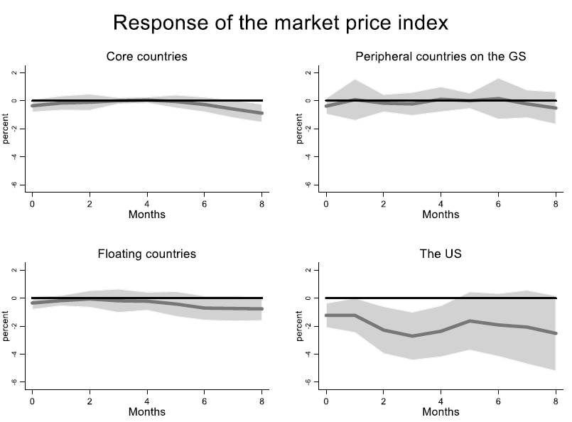
The responses of asset prices are consistent with our previous results and interpretation (Figure 5). In all countries with a central bank, we do not observe a significant response of asset prices to a rise in the BoE discount rate (and the central estimate is small). By contrast, the New York stock market reacts strongly to the BoE shock. At the 95 percent level, results are significant at the time of the shock and two to three months afterward (at a 90 percent confidence level, results are statistically significant continuously for six months). This dichotomyFootnote ³⁰ supports our main result, namely that central banks were able to act as a buffer, whereas in the absence of such an institution, the global financial cycle impacted on the domestic economy.

Figure 5

THE REACTION OF THE STOCK MARKET INDEX TO AN ENGLISH DISCOUNT RATE SHOCK OF 100 BASIS POINTS IN THE FIRST EIGHT MONTHS

Units: Percentage change compared to month t = –1.

Sources: Own calculations based on sources as described in the main text and the Online Appendix.

Arguments Based on Historical Narrative

Omitted variable bias occurs if the BoE rate reacts only to short-term shocks or cycles that are common to all countries. However, the high frequency of BoE rate changes does not suggest systematic simultaneity with global economic cycles and the policies of other central banks. During this period, the BoE changed its rate every two months on average, while, for example, the Bank of France—the second most important central bank—changed its rate once a year (Bazot, Bordo, and Monnet Reference Bazot, Bordo and Monnet2016). Furthermore, if relative purchasing power parity holds under the gold standard and BoE rate changes are linked to a global cycle in inflation rates, we should not observe a deviation of the exchange rate from mint parity: inflation and nominal interest rates should evolve in a similar way across gold standard countries, and the exchange rates remain fixed. Results in Figures 1 and 2 showed the contrary and should be interpreted as evidence that—at least in the short term—exchange-rate movements were driven by financial arbitrage rather than a global cycle.

As for reverse causality between central bank policy decisions, several authors have shown that the BoE was the first to move its rate among central banks (Lindert Reference Lindert1969; Eichengreen Reference Eichengreen1987; Morys Reference Morys2013; Bazot, Bordo, and Monnet Reference Bazot, Bordo and Monnet2016). Archival evidence on the days of discount rate changes (as gathered during our research) further supports the idea of a central bank time-tabling with an implicit hierarchy where London always met first. A change in the interest rate of the BoE was not sufficient to lead to changes in the rates of other central banks. But it typically precedes them.

Statistical Robustness Checks

In order to address these two issues with econometric techniques, we propose two robustness checks.

First, we include several additional variables in the estimations to control for potentially omitted variables, namely global cycles in prices, and economic or financial activity. For this period, monthly indices of economic activity are usually unavailable; exceptions are the English price index and a widely-used proxy of English domestic activity based on railway freight receipts constructed by Goodhart (Reference Goodhart1972). Furthermore, we use the stock market index in London as a measure of the financial cycle.Footnote ³¹ If there was any global cycle, it should be reflected in English macroeconomic and financial variables. Based on annual data, Morys and Ivanov (Reference Morys and Ivanov2015) provided new evidence that the English cycle was as close as possible to a global cycle during this period. In addition, we also control for English gold reserves, which might capture a global cycle in the gold supply. If the BoE reacted to a global shortage of gold (decreasing the gold stock of all central banks, including its own), we would over-estimate the reaction of gold reserves of other countries to an English interest rate shock.

Second, we address the reverse causality issue by using the exogenous measure of English monetary policy during the gold standard constructed by Lennard (Reference Lennard2018) following a narrative approach. Lennard (Reference Lennard2018) follows the seminal study of Romer and Romer (Reference Romer and Romer2004) by identifying the information set of the board members of the BoE based on a reading of transcripts of meetings. He then purged the BoE discount rate from the relevant information on expected economic changes that was available to policymakers at the time of decision making. The residuals identified at a decision-by-decision frequency are transformed into a monthly series by matching the shock with the month in which it occurred and summing shocks in months with multiple decisions. Among the 13 variables in the information set used by Lennard, some are domestic (stock prices, wheat prices), while others are international (gold reserves and exports, French and German discount rates and exchange rates, U.S. exchange rate).

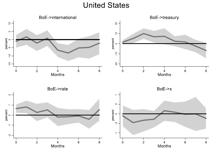
None of these two robustness tests change our previous conclusions, whether we introduce them separately or together. The only significant difference with our previous results concerns the United States in that it actually strengthens them. Thus we report here the new results for the United States only (Figure 6), while results for other countries are available in the Online Appendix (Figures A-9, A-10, and A-11). The effect of the English shock (1pp) on the U.S. interest rate is significantly stronger than in the benchmark estimate: 0.80pp after one month in Figure 6, compared to 0.49pp in Figure 4. Taking endogeneity into account leads to different results in the case of the United States only. The higher frequency of financial crises in the United States could explain why the endogeneity bias is stronger in this case: the BoE rate “overreacted” to changes in New York money market rates during such rare events.Footnote ³²

Figure 6

THE REACTION OF THE U.S. MONETARY SYSTEM TO AN ENGLISH DISCOUNT RATE SHOCK OF 100 BASIS POINTS IN THE FIRST EIGHT MONTHS. ALTERNATIVE MEASURE BASED ON LENNARD (Reference Lennard2018) AND ENGLISH CONTROL VARIABLES INCLUDED

Units: Percentage change compared to month t = –1 (positive exchange-rate response in lower right panel indicates depreciation).

Notes: “international” denotes the gold reserves of the U.S. Treasury, “rate” is the commercial paper rate in New York, and “x” the exchange rate in New York on London.

Sources: Own calculations based on sources as described in the main text and the Online Appendix.

We conducted an additional robustness check considering the specific case of the United States. The endogeneity issue is of particular concern in the case of the United States because this country experienced an unusual number of banking panics between 1890 and 1913, which impacted the English economy and pushed the BoE to increase its interest rate (Jeanne Reference Jeanne1995; Neal and Weidenmier Reference Neal, Weidenmier, Michael, Alan and Jeffrey2003; Hanes and Rhode Reference Hanes and Rhode2013). For this reason, Green (Reference Green2018) has built a specific measure of English monetary decisions that were unaffected by U.S. events. Based on the archives of the board meetings of the BoE, she identifies all discount rate changes motivated by a change in U.S. economic and financial conditions. Building on her work, we construct a discrete variable equal to 1 when BoE interest rate changes are exogenous to the U.S. economy and positive and –1 when they are negative. We then use this variable as an instrument to predict the series of actual BoE rate changes (see Jordà, Schularick, and Taylor Reference Jordà, Schularick and Taylor2020 for a presentation of IV in local projections).Footnote ³³ Results using exogenous Green shocks are consistent with those in Figure 6 using exogenous Lennard shocks (Online Appendix Figure A-12). The effect of the English shock (1pp) on the U.S. interest rate after one month is larger (0.61) than in our benchmark and increases steadily to 0.98 after four months.Footnote ³⁴