2.1. Constitutive behaviour of the phases

We assume that the suspended particles are homogeneous and made of deformable incompressible isotropic solids. We consider particles with viscoelastic behaviour and make use of a generalized KV model to describe their constitutive response. This model consists of a hyperelastic spring and a dashpot connected in parallel. (More general models, such as the Jeffreys model, could be considered at the expense of somewhat more complicated expressions.) We will also consider suspensions of purely elastic particles, which are one limiting case of KV particles. For the incompressible KV material, the Cauchy stress ${\bf\sigma}$ can be written as (Joseph Reference Joseph1990)

(2.1) $$\begin{eqnarray}{\bf\sigma}=-p_{0}\unicode[STIX]{x1D644}+{\bf\tau},\quad {\bf\tau}={\bf\tau}_{e}+{\bf\tau}_{v},\end{eqnarray}$$

where $p_{0}$ is an arbitrary hydrostatic pressure associated with the incompressibility constraint, and ${\bf\tau}_{e}$ and ${\bf\tau}_{v}$ are the elastic and viscous parts of the total ‘extra’ stress tensor ${\bf\tau}$ in the particle (which need not be deviatoric in general, $\text{tr}({\bf\tau})\neq 0$ ). It should be noted that the actual hydrostatic pressure $p$ is given by $p=p_{0}-\text{tr}\,{\bf\tau}$ .

The elastic stress may be described in terms of a stored-energy function ${\it\psi}$ , which, on account of frame invariance, is a function of $\unicode[STIX]{x1D63E}$ , via

(2.2a,b ) $$\begin{eqnarray}{\bf\tau}_{e}=2\unicode[STIX]{x1D641}\frac{\partial {\it\psi}(\unicode[STIX]{x1D63E})}{\partial \unicode[STIX]{x1D63E}}\unicode[STIX]{x1D641}^{\text{T}},\quad \det (\unicode[STIX]{x1D641})=1.\end{eqnarray}$$

In addition, elastic isotropy (and incompressibility) implies that ${\it\psi}$ depends on $\unicode[STIX]{x1D63E}$ through its first two invariants. For simplicity, in this work, we will consider generalized neo-Hookean behaviour such that ${\it\psi}(\unicode[STIX]{x1D63E})=g(I)$ , where $I=\text{tr}(\unicode[STIX]{x1D63E})$ and $g$ is a generally nonlinear function of $I$ satisfying the requirements that $g(3)=0,g^{\prime }(3)={\it\mu}/2$ , where ${\it\mu}$ is the ground-state shear modulus of the elastic particle. Then, the elastic extra stress tensor ${\bf\tau}_{e}$ in (2.2) can be expressed as

(2.3) $$\begin{eqnarray}{\bf\tau}_{e}=2\,g^{\prime }(I)\,\unicode[STIX]{x1D63D}-{\it\mu}\,\unicode[STIX]{x1D644},\end{eqnarray}$$

where the term proportional to ${\it\mu}$ arises from the linearization requirements at the ground state (i.e.  ${\bf\tau}_{e}(\unicode[STIX]{x1D644})=\mathbf{0}$ ).

Making use of the fact that (Joseph Reference Joseph1990)

(2.4) $$\begin{eqnarray}\stackrel{{\rm\nabla}}{\unicode[STIX]{x1D63D}}=\frac{\text{D}\unicode[STIX]{x1D63D}}{\text{D}t}-\unicode[STIX]{x1D647}\unicode[STIX]{x1D63D}-\unicode[STIX]{x1D63D}\unicode[STIX]{x1D647}^{\text{T}}=\mathbf{0},\end{eqnarray}$$

a rate (hypo-elastic) form of equation for the elastic constitutive relation (2.3) may be obtained in terms of the upper-convected (or Oldroyd) time derivative such that

(2.5) $$\begin{eqnarray}\stackrel{{\rm\nabla}}{{\bf\tau}}\text{}_{e}=\dot{{\bf\tau}}_{e}-\unicode[STIX]{x1D647}{\bf\tau}_{e}-{\bf\tau}_{e}\unicode[STIX]{x1D647}^{\text{T}}=4\,g^{\prime \prime }\,\text{tr}\left(\unicode[STIX]{x1D63F}\unicode[STIX]{x1D63D}\right)\unicode[STIX]{x1D63D}+2{\it\mu}\unicode[STIX]{x1D63F},\end{eqnarray}$$

where $\dot{{\bf\tau}}_{e}=(\partial {\bf\tau}_{e}/\partial t)+\boldsymbol{v}\boldsymbol{\cdot }\boldsymbol{{\rm\nabla}}{\bf\tau}_{e}$ denotes the material time derivative of the tensor ${\bf\tau}_{e}$ . For the more general elastic behaviour given by (2.2), corresponding expressions for the evolution of the extra stress may be found in the work of Bernstein (Reference Bernstein1960).

The simplest possible choice for the elastic behaviour of the particles is of course the neo-Hookean model with $g(I)={\it\mu}/2(I-3)$ . However, this model is unrealistic at large stretches for most materials, including elastomers, as it ignores the significant stiffening that such materials exhibit at large stretches. For this reason, in the applications to be considered below, we will make use of the Gent model (Gent Reference Gent1996), characterized by the choice

(2.6) $$\begin{eqnarray}g(I)=-\frac{J_{m}{\it\mu}}{2}\ln \left(1-\frac{I-3}{J_{m}}\right)\!,\end{eqnarray}$$

where the dimensionless parameter $J_{m}>0$ , known as the strain-locking parameter, corresponds to the limiting value of $I-3$ at which the elastomer locks up (and the argument of the logarithm vanishes). It should be noted that the Gent model (2.6) reduces to the neo-Hookean model in the limit as $J_{m}\rightarrow \infty$ . The corresponding specialization of the constitutive relation (2.3) can then be written as

(2.7) $$\begin{eqnarray}{\bf\tau}_{e}={\it\mu}\left[\left(1-\frac{I-3}{J_{m}}\right)^{-1}\unicode[STIX]{x1D63D}-\unicode[STIX]{x1D644}\right]\!,\end{eqnarray}$$

which in turn leads to the following evolution equation for the elastic extra stress tensor:

(2.8) $$\begin{eqnarray}\stackrel{{\rm\nabla}}{{\bf\tau}}\text{}_{e}=2{\it\mu}\unicode[STIX]{x1D63F}+\frac{2}{{\it\mu}J_{m}}\text{tr}\left[\unicode[STIX]{x1D63F}\left({\bf\tau}_{e}+{\it\mu}\unicode[STIX]{x1D644}\right)\right]\left({\bf\tau}_{e}+{\it\mu}\unicode[STIX]{x1D644}\right)\!,\end{eqnarray}$$

where use has been made of (2.7) to express $\unicode[STIX]{x1D63D}$ in terms of ${\bf\tau}_{e}$ . It should be noted that these expressions reduce to the well-known neo-Hookean expressions (Joseph Reference Joseph1990) in the limit as $J_{m}\rightarrow \infty$ , namely,

(2.9a,b ) $$\begin{eqnarray}{\bf\tau}_{e}={\it\mu}(\unicode[STIX]{x1D63D}-\unicode[STIX]{x1D644})\quad \text{and}\quad \stackrel{{\rm\nabla}}{{\bf\tau}}\text{}_{e}=2{\it\mu}\unicode[STIX]{x1D63F}.\end{eqnarray}$$

Going back to the general expressions for the KV material, the viscous part of the extra stress can likewise be described in terms of a dissipation potential ${\it\phi}$ , which, on account of incompressibility and frame invariance, is a function of the last two invariants of $\unicode[STIX]{x1D63F}$ , via

(2.10a,b ) $$\begin{eqnarray}{\bf\tau}_{v}=\frac{\partial {\it\phi}(\unicode[STIX]{x1D63F})}{\partial \unicode[STIX]{x1D63F}},\quad \text{tr}(\unicode[STIX]{x1D63F})=0.\end{eqnarray}$$

Although more general nonlinear forms could be considered, in this work, again for simplicity, we will focus our attention on linearly viscous behaviour, such that

(2.11) $$\begin{eqnarray}{\bf\tau}_{v}=2{\it\eta}^{(2)}\unicode[STIX]{x1D63F},\end{eqnarray}$$

where ${\it\eta}^{(2)}$ describes the constant viscosity of the particle material.

It should be noted that the set of constitutive relations for KV particles reduces to those for purely elastic particles by taking the limit as the viscosity ${\it\eta}^{(2)}$ goes to zero. In this limit, the KV model simplifies to a hyperelastic model characterized by the stored-energy function ${\it\psi}(\unicode[STIX]{x1D641})$ . In other words, in this limit, the viscous part of the stress vanishes ( ${\bf\tau}_{v}=\mathbf{0}$ ) and the elastic part coincides with the total stress ( ${\bf\tau}_{e}={\bf\tau}$ ). Therefore, for the case of (incompressible) Gent particles, the constitutive relation for the extra stress tensor ( ${\bf\tau}$ ) and its evolution ( $\stackrel{{\rm\nabla}}{{\bf\tau}}$ ) are given by (2.7) and (2.8) respectively, with ${\bf\tau}_{e}$ being replaced by ${\bf\tau}$ . These relations have been shown to provide good agreement with experimental data for rubber-like materials (Ogden, Saccomandi & Sgura Reference Ogden, Saccomandi and Sgura2004). Similarly, for the case of neo-Hookean particles, the corresponding relations are given by (2.9), with ${\bf\tau}_{e}$ being replaced by ${\bf\tau}$ . In addition, it should be noted that the constitutive relations for KV particles also reduce to those for purely viscous (Newtonian) particles by taking the limit as the shear modulus ${\it\mu}$ tends to zero. However, our main interest in this work is in ‘solid’ particles and we shall not consider this limit here, which would be more relevant for ‘fluid’ inclusions (droplets) in the context of emulsions.

The suspending fluid (or the matrix) will be assumed here to be an incompressible Newtonian fluid, with its constitutive relation given by expression (2.1) with

(2.12a,b ) $$\begin{eqnarray}{\bf\tau}={\bf\tau}_{v}=2{\it\eta}^{(1)}\unicode[STIX]{x1D63F},\quad \text{tr}(\unicode[STIX]{x1D63F})=0.\end{eqnarray}$$

In other words, the constitutive behaviour of the matrix will be taken to be purely viscous with linear response and constant viscosity ${\it\eta}^{(1)}$ .

2.2. Microstructures

In this paper, we confine our attention to suspensions consisting of initially spherical highly deformable viscoelastic solid particles that are distributed isotropically in a Newtonian viscous fluid (matrix). Based on earlier theoretical work for dilute concentrations of (non-interacting) deformable particles (Goddard & Miller Reference Goddard and Miller1967; Roscoe Reference Roscoe1967; Gao et al. Reference Gao, Hu and Ponte Castañeda2011, Reference Gao, Hu and Ponte Castañeda2013), the particles are expected to change their shape and orientation when subjected to a shear flow. As already mentioned, for dilute concentrations, the initial spherical particles become aligned ellipsoids with a shape and orientation that evolve with the deformation until (possibly) reaching a steady state. On the other hand, for non-dilute concentrations (see the numerical simulations of Clausen, Reasor & Aidun (Reference Clausen, Reasor and Aidun2011) for moderately concentrated suspensions of capsules), it may be expected that the shape assumed by the viscoelastic particles in our suspensions will not be precisely ellipsoidal – deviations would be expected due to the non-uniform deformation fields that would be generated inside the particles as a consequence of the particle interactions. In addition, it would be expected that the shape and orientation of all the particles in the suspension would not be precisely the same, due to differences in the local environments ‘seen’ by different particles. Nevertheless, in the spirit of generating simplified (homogenized) constitutive models for the instantaneous response of the non-dilute suspensions, as well as for the evolution of their microstructure, it makes sense to define suitable homogenized microstructural variables serving to characterize the evolution of the ‘average’ shape and orientation of the particles, as functions of the deformation. Similarly, the two- and higher-point correlation functions for the distribution of the particle centres would be expected to evolve in a complicated way with the deformation. However, once again in the spirit of developing homogenized rheological models, it is reasonable to make use of simplified assumptions for the evolution of such correlation functions.

In the context of purely viscous systems, and ignoring surface tension effects (i.e. distributions of viscous drops in a viscous fluid), Kailasam & Ponte Castañeda (Reference Kailasam and Ponte Castañeda1998) proposed such a model utilizing a suitable application/generalization of the homogenization estimates of Ponte Castañeda & Willis (Reference Ponte Castañeda and Willis1995) for the ‘macroscopic’ viscosity, as well as for the ‘average’ strain-rate and vorticity fields in the particle phase, to generate corresponding estimates for the instantaneous response of the suspension, as well as evolution laws for suitable microstructural variables characterizing the average shape and orientation of the particles, and of the two-point correlation functions describing the relative positions of the particles in the flow. In this context, it should be emphasized that the homogenization estimates of Ponte Castañeda & Willis (Reference Ponte Castañeda and Willis1995) provide a generalization of the dilute estimates of Eshelby (Reference Eshelby1957) for non-dilute dispersions of elastic particles in an elastic matrix (with different elastic moduli) – which can be reinterpreted for viscous particles in a viscous matrix – accounting for general ellipsoidal particle shapes distributed with generally different ellipsoidal shape for the two-point probability function for the particle-centre distribution. The constitutive theory of Kailasam & Ponte Castañeda (Reference Kailasam and Ponte Castañeda1998) applies not only for linearly viscous behaviour for the phases, but can also be used for nonlinearly viscous (including ideally plastic in the rate-independent limit) phases, and generalizes earlier work in this context by Kailasam et al. (Reference Kailasam, Ponte Castañeda and Willis1997) for the evolution of the particle shape and distribution (with fixed orientation). In this work, we propose a corresponding generalization of this theory to account for viscoelastic effects in the particles at non-dilute concentrations, building on the earlier work by Gao et al. (Reference Gao, Hu and Ponte Castañeda2011) for dilute concentrations of elastic particles. This will require extension of the notion of suitable microstructural variables to include the average elastic stress in the particles, as will be seen in more detail further below.

Consistent with the just-stated objectives, we define next a special class of microstructures characterizing the instantaneous state of the system. Thus, it is assumed that at the present time all the initially (at zero time) spherical particles become ellipsoidal with identical shape and orientation, as described by representative (average) ellipsoids

(2.13) $$\begin{eqnarray}{\it\Omega}^{(2)}=\left\{\boldsymbol{x}:|(\unicode[STIX]{x1D655})^{-\text{T}}\boldsymbol{x}|\leqslant 1\!\right\}\!,\end{eqnarray}$$

where $\unicode[STIX]{x1D655}$ is the so-called shape tensor. In addition, it will be assumed here that the relative position of the particles is described by two-point correlation functions having ‘ellipsoidal’ symmetry. This notion was introduced by Willis (Reference Willis1977) to describe the shape for the angular dependence of two-point correlation functions, thus generalizing the notion of ‘statistical isotropy’, which corresponds to spherical angular dependence. It was used in the work of Ponte Castañeda & Willis (Reference Ponte Castañeda and Willis1995) to describe the shape of the two-point probabilities for the distribution of the centres of ellipsoidal particles with possibly different shapes and orientations, thus resulting in estimates depending on two generally different Eshelby-type microstructural tensors, one describing the shape and orientation of the particles and the other those of their distribution. While in general it may be expected that the shape and orientation of the particle distribution will evolve differently from the shape and orientation of the particles themselves, in this first investigation of the problem, we will assume, for simplicity, that the shape and orientation of the distribution functions are identical to those of the individual particles. We expect this to be a reasonable approximation for small to moderate particle volume fractions for two reasons. First, the effect of the particle distribution is expected to be of the order of the volume fraction squared, while that of the particles themselves is expected to be of the order of the volume fraction. Therefore, the effect of the shape of the distribution functions is expected to be small compared with that of the particle shapes themselves, at least for small to moderate volume fractions. Second, the numerical simulations of Clausen et al. (Reference Clausen, Reasor and Aidun2011) for suspensions of concentrated capsules in a simple shear flow (see figures 11 and 13 in that paper) seem to suggest that this is not a bad approximation – certainly better than assuming that the distribution of the (non-Brownian) particles remains isotropic. Another possibility would be to assume that the shape and orientation of the particles evolve with the macroscopic deformation (Kailasam et al. Reference Kailasam, Ponte Castañeda and Willis1997), as would be the case for periodic distributions of particles, but such an approximation would only be accurate for small enough volume fractions, and will not be pursued in this work, again mostly for simplicity, as it is much easier to work with one shape tensor than with two.

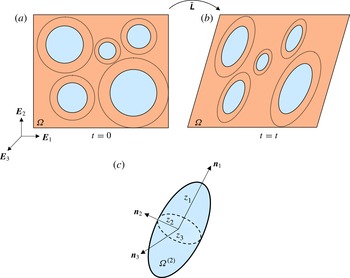
Figure 1(a) provides a schematic representation of the isotropic distribution of spherical particles in the suspension at $t=0$ . The spheres with solid and dotted lines represent cross-sections of the particles and the distributional spheres, respectively. The triad $\{\boldsymbol{E}_{i}\}$ ( $i=1,2,3$ ) is used to characterize the fixed laboratory coordinates. Figure 1(b) depicts a snapshot of the suitably idealized microstructure in the suspension at a future time instant $t$ (recall that the particles and distributional ellipsoids are assumed to have the same shape and orientation at any moment). Moreover, figure 1(c) provides a schematic representation of the relevant microstructural variables at time $t$ . The three orthonormal vectors $\boldsymbol{n}_{1}$ , $\boldsymbol{n}_{2}$ and $\boldsymbol{n}_{3}=\boldsymbol{n}_{1}\times \boldsymbol{n}_{2}$ are used to characterize the principal axes of the particle. In this principal coordinate system, the shape tensor $\unicode[STIX]{x1D655}$ has the matrix representation $\unicode[STIX]{x1D655}=\text{diag}(z_{1},z_{2},z_{3})$ , with $z_{1}$ , $z_{2}$ , $z_{3}$ being the three principal semi-axes of the ellipsoid. For future reference, it is convenient to define two aspect ratios

(2.14a,b ) $$\begin{eqnarray}w_{1}=z_{2}/z_{1}\quad \text{and}\quad w_{2}=z_{3}/z_{1},\end{eqnarray}$$

which fully characterize the shape of the particle.

Figure 1.

Schematic illustration of the microstructure in the suspension, identifying the various microstructural variables. The particle shapes and orientations evolve with the deformation and are depicted as grey ellipses, while their two-point probability functions are depicted as larger dotted ellipses surrounding the particles. (a) At $t=0$ , the particles are spherical and distributed randomly with statistical isotropy in the Newtonian fluid. (b) At a later time $t$ , after application of the macroscopic velocity gradient $\bar{\unicode[STIX]{x1D647}}$ , the particles have become ellipsoidal and are distributed with ellipsoidal symmetry (with the same shape and orientation). (c) The particles are described by a ‘representative ellipsoid’ with aspect ratios $w_{1}=z_{2}/z_{1}$ and $w_{2}=z_{3}/z_{1}$ , and with principal axes defined by the unit vectors $\boldsymbol{n}_{1}$ , $\boldsymbol{n}_{2}$ and $\boldsymbol{n}_{3}=\boldsymbol{n}_{1}\times \boldsymbol{n}_{2}$ (which rotate relative to the laboratory axes $\{\boldsymbol{E}_{i}\},i=1,2,3$ ).

Consistent with the above-described microstructural model, we choose the following set of variables to characterize the state of the ellipsoidal microstructure:

(2.15) $$\begin{eqnarray}\mathscr{S}=\{w_{1},w_{2},\boldsymbol{n}_{1},\boldsymbol{n}_{2},\boldsymbol{n}_{3}=\boldsymbol{n}_{1}\times \boldsymbol{n}_{2}\}.\end{eqnarray}$$

3.1. Homogenization estimates for the instantaneous response

We consider a representative volume element (RVE) of the suspension, which occupies a volume ${\it\Omega}$ with boundary $\partial {\it\Omega}$ . The fluid and particle phases are in turn assumed to occupy volumes ${\it\Omega}^{(1)}$ and ${\it\Omega}^{(2)}$ respectively, such that ${\it\Omega}={\it\Omega}^{(1)}+{\it\Omega}^{(2)}$ . It is assumed that the RVE satisfies the separation of length scales hypothesis, implying that the typical size of the neutrally buoyant particles is much smaller than the size of the RVE, as well as the Stokes condition in the fluid phase, such that

(3.1) $$\begin{eqnarray}\mathit{Re}=\frac{{\it\rho}^{(1)}\,\dot{{\it\gamma}}\,d_{p}^{2}}{{\it\eta}^{(1)}}\rightarrow 0,\end{eqnarray}$$

where ${\it\rho}^{(1)}$ is the density of the fluid, $\dot{{\it\gamma}}$ is a measure of the macroscopic strain rate and $d_{p}$ is a measure of the particle diameter. Noting that the microstructure of the RVE is statistically uniform, a uniform macroscopic stress field will be generated in the RVE when an affine velocity boundary condition is applied on the boundary of the RVE ( $\partial {\it\Omega}$ ). Thus, the suspension is subjected to the boundary condition

(3.2) $$\begin{eqnarray}\boldsymbol{v}(\boldsymbol{x})=\bar{\unicode[STIX]{x1D647}}\,\boldsymbol{x},\quad \text{on }\partial {\it\Omega},\end{eqnarray}$$

where $\bar{\unicode[STIX]{x1D647}}~(\text{tr}\,\bar{\unicode[STIX]{x1D647}}=0)$ is the macroscopic, or average, velocity gradient, defined by

(3.3) $$\begin{eqnarray}\bar{\unicode[STIX]{x1D647}}=\frac{1}{\text{Vol}({\it\Omega})}\int _{{\it\Omega}}\unicode[STIX]{x1D647}\,\text{d}V.\end{eqnarray}$$

(This follows from the mean value theorem for the strain rate, e.g. Ponte Castañeda & Suquet, Reference Ponte Castañeda and Suquet1998, which states that the volume average of the local strain-rate tensor $\unicode[STIX]{x1D647}$ over the RVE under the affine velocity boundary condition (3.2) is precisely $\bar{\unicode[STIX]{x1D647}}$ .) Similarly, the average or macroscopic Cauchy stress is defined as

(3.4) $$\begin{eqnarray}\bar{{\bf\sigma}}=\frac{1}{\text{Vol}({\it\Omega})}\int _{{\it\Omega}}{\bf\sigma}\text{d}V,\end{eqnarray}$$

and the instantaneous macroscopic constitutive response is determined by the relation between $\bar{{\bf\sigma}}$ and $\bar{\unicode[STIX]{x1D647}}$ .

For future reference, we also define the phase averages of the strain-rate field over phase $r~(r=1,2)$ via

(3.5) $$\begin{eqnarray}\bar{\unicode[STIX]{x1D63F}}^{(r)}=\frac{1}{\text{Vol}({\it\Omega}^{(r)})}\int _{{\it\Omega}^{(r)}}\,\unicode[STIX]{x1D63F}\,\text{d}V,\end{eqnarray}$$

such that

(3.6) $$\begin{eqnarray}\bar{\unicode[STIX]{x1D63F}}=c^{(1)}\bar{\unicode[STIX]{x1D63F}}^{(1)}+c^{(2)}\,\bar{\unicode[STIX]{x1D63F}}^{(2)},\end{eqnarray}$$

with the $c^{(1)}$ and $c^{(2)}$ denoting the volume fractions of the fluid and particle phases respectively. Similarly, defining $\bar{{\bf\tau}}^{(1)}$ and $\bar{{\bf\tau}}^{(2)}$ as the averages of the extra stress in the fluid and particle phases respectively, the macroscopic stress, as defined by (3.4), can be rewritten (on account of the incompressibility of the phases) as

(3.7) $$\begin{eqnarray}\bar{{\bf\sigma}}=-\bar{p}_{0}\,\unicode[STIX]{x1D644}+c^{(1)}\,\bar{{\bf\tau}}^{(1)}+c^{(2)}\,\bar{{\bf\tau}}^{(2)},\end{eqnarray}$$

where $\bar{p}_{0}$ is an indeterminate hydrostatic pressure associated with the overall incompressibility of the suspension. It should be noted that the effect of the compressibility of the bulk fluid has been considered by Brady, Khair & Swaroop (Reference Brady, Khair and Swaroop2006) in the context of suspensions of rigid spherical particles.

Now, taking advantage of the special form of the constitutive relations for the fluid matrix and solid particle phases, as described in § 2.1, pseudo-dissipation potentials are introduced:

(3.8a,b ) $$\begin{eqnarray}W^{(r)}(\unicode[STIX]{x1D63F})={\it\eta}^{(r)}\unicode[STIX]{x1D63F}\boldsymbol{\cdot }\unicode[STIX]{x1D63F}+{\bf\tau}_{e}\boldsymbol{\cdot }\unicode[STIX]{x1D63F},\quad \text{tr}(\unicode[STIX]{x1D63F})=0,\end{eqnarray}$$

such that the local constitutive relation of the phases can be written as

(3.9a,b ) $$\begin{eqnarray}{\bf\sigma}=-p_{0}\,\unicode[STIX]{x1D644}+{\bf\tau},\quad \text{where }{\bf\tau}=\frac{\partial W^{(r)}}{\partial \unicode[STIX]{x1D63F}}=2\,{\it\eta}^{(r)}\unicode[STIX]{x1D63F}+{\bf\tau}_{e}.\end{eqnarray}$$

Here, $p_{0}$ is an indeterminate hydrostatic pressure. It should also be emphasized that the elastic strains ${\bf\tau}_{e}$ are considered to be fixed in taking the derivative with respect to $\unicode[STIX]{x1D63F}$ . Thus, it can be seen that the addition of the linear term in the strain-rate tensor $\unicode[STIX]{x1D63F}$ to the dissipation function ${\it\phi}$ , defined by (2.10), allows the inclusion of the elastic stress ${\bf\tau}_{e}$ , assuming that it is known at the given instant. More specifically, labelling the quantities associated with the matrix and particle phases by the superscripts (1) and (2) respectively, the local constitutive relation (3.9) can be used to recover the constitutive relations for the elastic particles and fluid matrix phases, as given by (2.1)–(2.12), provided that we let ${\it\eta}^{(1)}$ and ${\it\eta}^{(2)}$ be the viscosities of the fluid and elastic particles respectively, and that we let ${\bf\tau}_{e}=0$ in the fluid phase and ${\bf\tau}_{e}={\bf\tau}_{e}^{(2)}$ , as characterized by the evolution equation (2.8), in the particle phase. In addition, in this last expression, we use ${\it\mu}$ and $J_{m}$ to describe the ground shear modulus and strain-locking parameter of the elastic particles, the superscript (2) having been dropped from ${\it\mu}$ and $J_{m}$ for convenience (since only the particle phase has elastic properties, thus eliminating the risk of confusion).

We define next, for compactness, the local pseudo-dissipation potential

(3.10) $$\begin{eqnarray}W(\boldsymbol{x},\unicode[STIX]{x1D63F})={\it\chi}^{(1)}(\boldsymbol{x})W^{(1)}(\unicode[STIX]{x1D63F})+{\it\chi}^{(2)}(\boldsymbol{x})W^{(2)}(\unicode[STIX]{x1D63F}),\end{eqnarray}$$

where the ${\it\chi}^{(r)}(\boldsymbol{x})~(r=1,2)$ are the characteristic functions of the two phases, such that they are equal to one if the position vector $\boldsymbol{x}$ is in phase $r$ (i.e.  $\boldsymbol{x}\in {\it\Omega}^{(r)}$ ) and zero otherwise. Then, we can state the principle of minimum dissipation (see Keller et al. Reference Keller, Rubenfeld and Molyneux1967) via

(3.11) $$\begin{eqnarray}\min _{\unicode[STIX]{x1D63F}\in K}\int _{{\it\Omega}}W(\boldsymbol{x},\unicode[STIX]{x1D63F})\text{d}V,\end{eqnarray}$$

where $K$ denotes the set of kinematically admissible strain rates:

(3.12) $$\begin{eqnarray}K=\{\unicode[STIX]{x1D63F}\mid \text{there is }\boldsymbol{v}\text{ such that }\unicode[STIX]{x1D63F}=(\boldsymbol{{\rm\nabla}}\boldsymbol{v}+(\boldsymbol{{\rm\nabla}}\boldsymbol{v})^{\text{T}})/2,\text{div}\,\boldsymbol{v}=0\text{ in }{\it\Omega},\text{and }\boldsymbol{v}=\bar{\unicode[STIX]{x1D647}}\boldsymbol{x}\text{ on }\partial {\it\Omega}\}.\end{eqnarray}$$

It is noted (see Ekeland & Témam Reference Ekeland and Témam1999, for the purely viscous problem) that the Euler–Lagrange equations of this variational principle are precisely the Stokes equations for the fluid phase,

(3.13a,b ) $$\begin{eqnarray}2\,{\it\eta}^{(1)}{\rm\nabla}^{2}\boldsymbol{v}-\boldsymbol{{\rm\nabla}}p=\mathbf{0},\quad \boldsymbol{{\rm\nabla}}\boldsymbol{\cdot }\boldsymbol{v}=0,\end{eqnarray}$$

together with the equilibrium equations for the solid particles, which in Eulerian form become

(3.14a,b ) $$\begin{eqnarray}2\,{\it\eta}^{(2)}{\rm\nabla}^{2}\boldsymbol{v}-\boldsymbol{{\rm\nabla}}p_{0}+\boldsymbol{{\rm\nabla}}\boldsymbol{\cdot }{\bf\tau}_{e}^{(2)}=\mathbf{0},\quad \boldsymbol{{\rm\nabla}}\boldsymbol{\cdot }\boldsymbol{v}=0,\end{eqnarray}$$

where once again the elastic extra stress ${\bf\tau}_{e}^{(2)}$ in the particles is assumed to be known at the present instant. It should be mentioned that the variational principle also ensures continuity of the velocity $\boldsymbol{v}$ and traction components of the total stress ${\bf\sigma}$ across the particle–fluid boundaries, as well as satisfaction of the affine boundary condition (3.2).

Finally, it is noted that the dissipation functional in (3.11), evaluated at the minimum, defines a function of the macroscopic strain rate $\bar{\unicode[STIX]{x1D63F}}$ , as given by the symmetric part of the average velocity gradient $\bar{\unicode[STIX]{x1D647}}$ . When normalized by the volume of the RVE ${\it\Omega}$ , it can be shown (see, for example, Ponte Castañeda & Suquet Reference Ponte Castañeda and Suquet1998) that it provides a pseudo-dissipation potential for the macroscopic constitutive relation, in the sense that

(3.15) $$\begin{eqnarray}\bar{{\bf\sigma}}=-\bar{p}_{0}\,\unicode[STIX]{x1D644}+\bar{{\bf\tau}},\quad \text{where }\bar{{\bf\tau}}=\frac{\partial \widetilde{W}}{\partial \bar{\unicode[STIX]{x1D63F}}},\end{eqnarray}$$

and where $\bar{p}_{0}$ is the Lagrange multiplier associated with the macroscopic incompressibility constraint and

(3.16) $$\begin{eqnarray}\widetilde{W}(\bar{\unicode[STIX]{x1D63F}})=\min _{\unicode[STIX]{x1D63F}\in K}\,\frac{1}{\text{Vol}({\it\Omega})}\,\int _{{\it\Omega}}W(\boldsymbol{x},\unicode[STIX]{x1D63F})\text{d}V.\end{eqnarray}$$

The homogenization problem defined by (3.15) and (3.16) for the instantaneous response of the viscoelastic composite characterized by (3.8)–(3.10) is mathematically analogous to the corresponding problem for an incompressible thermoelastic composite with ‘elastic moduli’ ${\it\eta}^{(r)}$ and ‘thermal stresses’ ${\bf\tau}_{e}$ (provided that the strain-rate and velocity fields are identified with the ‘strain’ and ‘displacement’ fields, respectively). For the specific problem of interest here, the viscosities (moduli) ${\it\eta}^{(r)}$ are uniform-per-phase, and while the elastic stress (thermal stress) in the matrix phase is zero, the corresponding elastic stress (thermal stress) in the particle phase is not only non-vanishing, but in fact also non-uniform. More general situations, including the case of non-uniform thermal stresses in the matrix phase, have been considered recently by Lahellec, Ponte Castañeda & Suquet (Reference Lahellec, Ponte Castañeda and Suquet2011).

To estimate the effective dissipation function $\widetilde{W}(\bar{\unicode[STIX]{x1D63F}})$ , we make use of the HSW variational method, which was originally developed for isotropic linear-elastic composites by Hashin & Shtrikman (Reference Hashin and Shtrikman1963), and extended later for generally anisotropic linear-elastic composites by Willis (Reference Willis1977, Reference Willis1981). For the particulate material systems of interest in this work consisting of random distributions of ellipsoidal inclusions in a given matrix, more explicit estimates have been given by Ponte Castañeda & Willis (Reference Ponte Castañeda and Willis1995) still making use of the HSW variational method. When applied to the above-described viscous systems, the key feature of this method is the use of a ‘polarization field’ relative to a homogeneous ‘comparison fluid’ (with viscosity ${\it\eta}^{0}$ ). By means of this subterfuge, it is possible to make use of simple constant-per-phase trial fields for the stress polarization to obtain bounds and estimates for the effective response of the composite system, which only depend on the appropriate first- and second-order statistics of the microstructure (i.e. the volume fraction and average shape and orientation of the particles, as well as the ‘shape’ and ‘orientation’ of the two-point statistics for the particle centres). The application of the method of Ponte Castañeda and Willis (PCW) to the class of suspensions of ‘thermoelastic’ particles of interest in this work was given by Ponte Castañeda (Reference Ponte Castañeda2005). For completeness, the adaptation of these results to the above-defined problem for suspensions of viscoelastic particles is given in appendix A. In this section, we will only provide the final results for the macroscopic response, as well as for the average strain-rate and vorticity fields in the particle phase.

Thus, the resulting variational estimate for the effective dissipation function $\widetilde{W}(\bar{\unicode[STIX]{x1D63F}})$ can be expressed as

(3.17) $$\begin{eqnarray}\widetilde{W}(\bar{\unicode[STIX]{x1D63F}})={\it\eta}^{(1)}\bar{\unicode[STIX]{x1D63F}}\boldsymbol{\cdot }\bar{\unicode[STIX]{x1D63F}}+c\left({\it\eta}^{(2)}-{\it\eta}^{(1)}\right)\bar{\unicode[STIX]{x1D63F}}^{(2)}\boldsymbol{\cdot }\bar{\unicode[STIX]{x1D63F}}+\frac{c}{2}\,\bar{{\bf\tau}}_{e}^{(2)}\boldsymbol{\cdot }(\bar{\unicode[STIX]{x1D63F}}^{(2)}+\bar{\unicode[STIX]{x1D63F}}),\end{eqnarray}$$

where

(3.18) $$\begin{eqnarray}\bar{\unicode[STIX]{x1D63F}}^{(2)}=\left\{\unicode[STIX]{x1D644}-2\,(1-c)\left({\it\eta}^{(1)}-{\it\eta}^{(2)}\right)\unicode[STIX]{x1D64B}\right\}^{-1}\left\{\bar{\unicode[STIX]{x1D63F}}-(1-c)\,\unicode[STIX]{x1D64B}\,\bar{{\bf\tau}}_{e}^{(2)}\right\}\end{eqnarray}$$

is the corresponding estimate for the average strain rate over the particles. In these expressions, it is recalled from appendix A that $c=c^{(2)}$ is the volume fraction of the particle phase, $\bar{{\bf\tau}}_{e}^{(2)}$ is the average elastic stress in the particles and $\unicode[STIX]{x1D64B}$ is a microstructural (Eshelby-type) tensor given by (A 11a ).

For later reference, we note that the procedure also provides an estimate for the average vorticity tensor in the particle phase (see appendix A), which is given by

(3.19) $$\begin{eqnarray}\bar{\unicode[STIX]{x1D652}}^{(2)}=\bar{\unicode[STIX]{x1D652}}+(1-c)\,\unicode[STIX]{x1D64D}\left[2\left({\it\eta}^{(1)}-{\it\eta}^{(2)}\right)\bar{\unicode[STIX]{x1D63F}}^{(2)}-\bar{{\bf\tau}}_{e}^{(2)}\right]\!,\end{eqnarray}$$

where $\unicode[STIX]{x1D64D}$ is the microstructural tensor defined by (A 11b ).

Finally, the instantaneous macroscopic constitutive relation for the suspension of viscoelastic particles can be obtained from the estimate (3.17) for $\widetilde{W}(\bar{\unicode[STIX]{x1D63F}})$ by means of (3.15). However, given $\bar{\unicode[STIX]{x1D63F}}^{(2)}$ and $\bar{{\bf\tau}}_{e}^{(2)}$ , it is simpler to make use of (3.6) to write the average extra stress in the matrix phase as

(3.20) $$\begin{eqnarray}\bar{{\bf\tau}}^{(1)}=2\,{\it\eta}^{(1)}\bar{\unicode[STIX]{x1D63F}}^{(1)}=2\,{\it\eta}^{(1)}\,(1-c)^{-1}(\bar{\unicode[STIX]{x1D63F}}-c\,\bar{\unicode[STIX]{x1D63F}}^{(2)}).\end{eqnarray}$$

Then, substituting this expression into expression (3.7) for the macroscopic stress, we arrive at

(3.21) $$\begin{eqnarray}\bar{{\bf\sigma}}=-\bar{p}\,\unicode[STIX]{x1D644}+2\,{\it\eta}^{(1)}\bar{\unicode[STIX]{x1D63F}}+c(\bar{{\bf\tau}}^{(2)}-2\,{\it\eta}^{(1)}\bar{\unicode[STIX]{x1D63F}}^{(2)}),\end{eqnarray}$$

which, using (3.9b ) to express the average extra stress over the inclusion phase in terms of the extra elastic stress over the particles, finally leads to

(3.22) $$\begin{eqnarray}\bar{{\bf\sigma}}=-\bar{p}_{0}\,\unicode[STIX]{x1D644}+2\,{\it\eta}^{(1)}\bar{\unicode[STIX]{x1D63F}}+2\,c\left({\it\eta}^{(2)}-{\it\eta}^{(1)}\right)\bar{\unicode[STIX]{x1D63F}}^{(2)}+c\,\bar{{\bf\tau}}_{e}^{(2)}.\end{eqnarray}$$

Thus, it can be seen that for given macroscopic strain rate $\bar{\unicode[STIX]{x1D63F}}$ , particle volume fraction $c$ and viscosities ${\it\eta}^{(1)}$ and ${\it\eta}^{(2)}$ , the macroscopic Cauchy stress tensor $\bar{{\bf\sigma}}$ may be determined from expression (3.22), by means of expression (3.18) for $\bar{\unicode[STIX]{x1D63F}}^{(2)}$ in terms of the current value of the average of the extra stress tensor over the particle $\bar{{\bf\tau}}_{e}^{(2)}$ , together with the current values of the average aspect ratios and orientation angles of the particles, as defined by expression (2.15). It should be emphasized that the above results reduce to the corresponding exact results of Gao et al. (Reference Gao, Hu and Ponte Castañeda2011) for dilute concentrations ( $c\ll 1$ ) and vanishing viscosity ( ${\it\eta}^{(2)}=0$ ) of the particles. (However, the results can also be shown to be exact for dilute concentrations of KV and other more general types of viscoelastic particles.) In the next subsection, we address the characterization of these variables by means of appropriate evolution equations, starting from an appropriate initial state where the particles are initially spherical and unstressed.

3.2. Evolution equations for the microstructural variables and particle elastic stress

So far, we have made use of Eulerian kinematics to describe the incremental behaviour of the host fluid and particle phases, and accordingly generated estimates for the instantaneous response of the suspension for a given state of the microstructure. However, when subjected to simple flows, the microstructure in the suspension generally evolves in time as the applied deformation progresses. Therefore, in order to predict the effective time-dependent behaviour of suspensions from a given initial state of the microstructure, it is crucial to first characterize the evolution of relevant microstructural variables. In addition, given that the instantaneous response depends on the current values of elastic stresses acting on the particles, which are determined by incremental constitutive equations of the type (2.8), it is also necessary to develop evolution laws for the average elastic stresses in the particles. As already anticipated in § 2.2, the initially spherical particles will deform – on average – through a sequence of ellipsoidal shapes throughout the deformation process. The average shape and orientation of the particles will be determined by standard kinematic arguments from expressions (3.18) and (3.19) for the instantaneous values of the average strain rate and vorticity in the inclusion phase. In this connection, it is important to emphasize that the above expressions for the instantaneous average strain rate and vorticity inside particles will continue to apply at each increment of time, except that at each step the current values of the microstructural variables and elastic stresses in the particles will need to be used. It is also recalled from § 2.2 that, for simplicity, the ‘shape’ and ‘orientation’ of the angular dependence of the two-point correlation functions for the distribution of the particle centres will be assumed in this first work to be identical to the average shape and orientation of the particles themselves. As already mentioned, this reduces the number of microstructural variables required, and results in considerable simplification of the constitutive model.

First, recalling that the fluid and particle phases have been assumed to be incompressible, it follows that the volume fraction of the particles will remain constant throughout any deformation process, i.e.

(3.23) $$\begin{eqnarray}c=\text{const}.\end{eqnarray}$$

On the other hand, the evolutions of the particle aspect ratios $w_{1}$ and $w_{2}$ , as defined by (2.14), are obtained by identifying the rate of change of the stretch of the particle along its principal axes with the appropriate normal components of the average strain-rate tensor in the particles, such that (see, for example, Bilby & Kolbuszewski Reference Bilby and Kolbuszewski1977)

(3.24a,b ) $$\begin{eqnarray}{\dot{w}}_{1}=w_{1}(\bar{\unicode[STIX]{x1D60B}}_{22}^{(2)}-\bar{\unicode[STIX]{x1D60B}}_{11}^{(2)}),\quad {\dot{w}}_{2}=w_{2}(\bar{\unicode[STIX]{x1D60B}}_{33}^{(2)}-\bar{\unicode[STIX]{x1D60B}}_{11}^{(2)}),\end{eqnarray}$$

where it is noted that the overdot here denotes simple time derivatives (since $w_{1}$ and $w_{2}$ depend only on time). It is also remarked in this context that the components of the tensorial variables associated with the particle phase, here and elsewhere, are referred to the principal axes of the ellipsoidal particle in their current state, as given by the triad $\{\boldsymbol{n}_{1},\boldsymbol{n}_{2},\boldsymbol{n}_{3}\}$ .

Next, the evolutions of the orthonormal vectors $\boldsymbol{n}_{1}$ , $\boldsymbol{n}_{2}$ and $\boldsymbol{n}_{3}$ , serving to characterize the orientation of particles, are determined by means of the kinematical relations

(3.25) $$\begin{eqnarray}\dot{\boldsymbol{n}}_{i}={\it\bf\Omega}\,\boldsymbol{n}_{i},\quad i=1,2,3,\end{eqnarray}$$

where ${\it\bf\Omega}$ is the (antisymmetric) spin tensor of the particle, whose components in the principal coordinate system $\{\boldsymbol{n}_{1},\boldsymbol{n}_{2},\boldsymbol{n}_{3}\}$ are determined in terms of the average strain rate and vorticity in the particles by means of the following relations (Kailasam & Ponte Castañeda Reference Kailasam and Ponte Castañeda1998; Aravas & Ponte Castañeda Reference Aravas and Ponte Castañeda2004):

(3.26) $$\begin{eqnarray}{\it\Omega}_{ij}=\bar{\unicode[STIX]{x1D61E}}_{ij}^{(2)}-\frac{\left(w_{i-1}\right)^{2}+(w_{j-1})^{2}}{\left(w_{i-1}\right)^{2}-(w_{j-1})^{2}}\,\bar{\unicode[STIX]{x1D60B}}_{ij}^{(2)},\quad i\neq j.\end{eqnarray}$$

In this notation, when $i$ or $j$ is equal to 1, we define $w_{1-1}=w_{0}=1$ . It should also be noted that alternative expressions for the evolution of the microstructure can be derived directly in terms of the particle shape tensors $\unicode[STIX]{x1D655}$ , as shown by Goddard & Miller (Reference Goddard and Miller1967).

As can be seen from relations (3.22), together with (3.18), the calculation of the instantaneous macroscopic stress in the suspension requires knowledge of the average elastic extra stress in the particle phase. As discussed in appendix A, due to the choice of constant-per-phase polarization fields, together with the choice of ${\it\eta}^{0}={\it\eta}^{(1)}$ , the PCW homogenization theory results in uniform stress and strain fields in the particle phase. As a consequence of this result, the constitutive relations for the average elastic stress fields in the particle phase take the same form as the corresponding relations for the local fields. Therefore, for the case of KV particles with a Gent-type elastic stress (characterized by relations (2.7) and (2.8)), the evolution equation for the average elastic extra stress in the particles is given by

(3.27) $$\begin{eqnarray}\displaystyle \stackrel{{\rm\nabla}}{\bar{{\bf\tau}}}\text{}_{e}^{(2)} & = & \displaystyle \dot{\bar{{\bf\tau}}}_{e}^{(2)}-\bar{\unicode[STIX]{x1D647}}^{(2)}\bar{{\bf\tau}}_{e}^{(2)}-\bar{{\bf\tau}}_{e}^{(2)}(\bar{\unicode[STIX]{x1D647}}^{(2)})^{\text{T}}\nonumber\\ \displaystyle & = & \displaystyle 2{\it\mu}\bar{\unicode[STIX]{x1D63F}}^{(2)}+\frac{2}{{\it\mu}\,J_{m}}\text{tr}\left[\bar{\unicode[STIX]{x1D63F}}^{(2)}\left(\bar{{\bf\tau}}_{e}^{(2)}+{\it\mu}\unicode[STIX]{x1D644}\right)\right]\left(\bar{{\bf\tau}}_{e}^{(2)}+{\it\mu}\unicode[STIX]{x1D644}\right)\!,\end{eqnarray}$$

where the material time derivative $\dot{\bar{{\bf\tau}}}_{e}^{(2)}$ appearing in the above expression is a simple time derivative, due to the fact that the stress field inside the particle is uniform (as already mentioned) and the convective terms hence vanish. It should be noted that the corresponding ‘integral’ form of the constitutive equation is given by

(3.28a,b ) $$\begin{eqnarray}\bar{{\bf\tau}}_{e}^{(2)}={\it\mu}\left[\left(1-\frac{\bar{I}^{(2)}-3}{J_{m}}\right)^{-1}\bar{\unicode[STIX]{x1D63D}}^{(2)}-\unicode[STIX]{x1D644}\right]\!,\quad \bar{{\bf\tau}}_{v}^{(2)}=2\,{\it\eta}^{(2)}\,\bar{\unicode[STIX]{x1D63F}}^{(2)},\end{eqnarray}$$

where $\bar{I}^{(2)}=\text{tr}(\bar{\unicode[STIX]{x1D63D}}^{(2)})$ , $\bar{\unicode[STIX]{x1D63D}}^{(2)}=\bar{\unicode[STIX]{x1D641}}^{(2)}(\bar{\unicode[STIX]{x1D641}}^{(2)})^{\text{T}}$ and $\bar{\unicode[STIX]{x1D641}}^{(2)}$ is the average deformation gradient in the particles.

It should also be noted that, in the limit as $J_{m}\rightarrow \infty$ (corresponding to KV particles with a neo-Hookean elastic part), the above evolution equation simplifies to

(3.29) $$\begin{eqnarray}\stackrel{{\rm\nabla}}{\bar{{\bf\tau}}}\text{}_{e}^{(2)}=2{\it\mu}\bar{\unicode[STIX]{x1D63F}}^{(2)}.\end{eqnarray}$$

In summary, for a given macroscopic velocity gradient $\bar{\unicode[STIX]{x1D647}}=\bar{\unicode[STIX]{x1D63F}}+\bar{\unicode[STIX]{x1D652}}$ , the macroscopic stress $\bar{{\bf\sigma}}$ in the suspension is given by (3.22), where $\bar{\unicode[STIX]{x1D63F}}^{(2)}$ is given by (3.18). These quantities depend on the particle volume fraction $c$ and on the current values of the microstructural variables $\mathscr{S}$ , as defined by (2.15), and determined by the evolution equations (3.24) and (3.25) from some known initial state, as well as on the current value of the average extra elastic stress $\bar{{\bf\tau}}_{e}^{(2)}$ in the particles, as determined by (3.27). It should be noted that the evolution equation for the particle axes (3.25) involves the average vorticity tensor in the particles, which is given in terms of other ‘known’ variables at the given time instant by (3.19). Due to the complex dependence of the microstructural tensors $\unicode[STIX]{x1D64B}$ and $\unicode[STIX]{x1D64D}$ on the microstructural variables $\mathscr{S}$ , it is not, in general, possible to simplify these expressions further.

In the context of the above-developed rheological model for dispersions of viscoelastic solid particles, it is important to emphasize that although the exact solution for the fields in the particles is not uniform in general, the uniform-field approximation in the inclusion phase is exact for dilute concentrations of particles ( $c\ll 1$ ), as originally argued by Roscoe (Reference Roscoe1967) for the SS solutions (when available) and shown by Gao et al. (Reference Gao, Hu and Ponte Castañeda2011) for more general time-dependent motions of dilute suspensions of purely elastic particles ( ${\it\eta}^{(2)}=0$ ). (The work of Gao et al. (Reference Gao, Hu and Ponte Castañeda2011) can be easily generalized to consider more general types of viscoelastic behaviour for the particles, including the KV model used in this work.) For non-dilute concentrations of particles, it is expected that the approximation of uniform fields in the particles will lead to fairly accurate results for low to moderate concentrations. However, as already mentioned, although serving to provide bounds for both poly- and monodisperse microstructures, the PCW-type estimates on which the model is based are more appropriate for polydisperse microstructures. For these reasons, it would be expected that the domain of application of the above-developed model for suspensions of elastic particles would be larger for polydisperse suspensions than for monodisperse suspensions. For related reasons, the homogenization model cannot handle strong interaction effects among the particles, such as the formation of clusters, which would be expected for monodisperse systems at sufficiently high concentrations. Finally, it should be remarked that in the limit as the shear modulus of the particles ${\it\mu}$ tends to zero, the constitutive model developed in the present work formally reduces to corresponding models developed by Kailasam & Ponte Castañeda (Reference Kailasam and Ponte Castañeda1998) for non-dilute dispersions of viscous particles (and, therefore, also to the results of Wetzel & Tucker Reference Wetzel and Tucker2001, for dilute dispersions of such particles). However, in spite of their theoretical interest, such models do not account for the effects of surface tension at the droplet–matrix interfaces, and as such cannot be used in practice as constitutive models for emulsions. In fact, the main objective of the work of Kailasam & Ponte Castañeda (Reference Kailasam and Ponte Castañeda1998) was to develop nonlinear constitutive models for the high-temperature creep (or high-strain-rate flow) of two-phase metals or rocks, where the viscous response of the phases can be described by nonlinear (power-law) constitutive laws, and interfacial tension can be neglected.

4.1. Steady-state solution for KV particles

In this subsection, we consider SS solutions in non-dilute suspensions of KV particles, characterized by the constitutive equations (3.28). Making use of (4.3) in (3.28a ), we find that the shear components of the elastic extra stress tensor (relative to the particle axes) are zero at the SS solution:

(4.7) $$\begin{eqnarray}(\bar{{\it\tau}}_{e}^{(2)})_{12}=(\bar{{\it\tau}}_{e}^{(2)})_{13}=(\bar{{\it\tau}}_{e}^{(2)})_{23}=0.\end{eqnarray}$$

Similarly, we find the three remaining (normal) components of the elastic extra stress tensor by making use of (4.6) in the constitutive relation (3.28a ). The final results read as

(4.8) $$\begin{eqnarray}\left.\begin{array}{@{}l@{}}(\bar{{\it\tau}}_{e}^{(2)})_{11}={\it\mu}\,d_{w}\!\left\{J_{m}\,(w_{2})^{1/3}\left[1-\left(w_{1}\,w_{2}\right)^{2/3}\right]+c_{w}\right\}\!,\\ (\bar{{\it\tau}}_{e}^{(2)})_{22}={\it\mu}\,d_{w}\!\left\{J_{m}\,(w_{2})^{1/3}\left[(w_{1})^{2}-\left(w_{1}\,w_{2}\right)^{2/3}\right]+c_{w}\right\}\!,\\ (\bar{{\it\tau}}_{e}^{(2)})_{33}={\it\mu}\,d_{w}\!\left\{J_{m}\,(w_{2})^{1/3}\left[(w_{2})^{2}-\left(w_{1}\,w_{2}\right)^{2/3}\right]+c_{w}\right\}\!,\end{array}\right\}\end{eqnarray}$$

where $c_{w}=(w_{2})^{1/3}[(w_{1})^{2}+(w_{2})^{2}+1]-3\,(w_{1})^{2/3}\,w_{2}$ and $d_{w}=[J_{m}\,(w_{1})^{2/3}\,w_{2}-c_{w}]^{-1}$ . In the limit as $J_{m}\rightarrow \infty$ (corresponding to KV particles with neo-Hookean elastic behaviour), the relations (4.8) simplify to

(4.9) $$\begin{eqnarray}\left.\begin{array}{@{}c@{}}(\bar{{\it\tau}}_{e}^{(2)})_{11}={\it\mu}\!\left[\left(w_{1}\,w_{2}\right)^{-2/3}-1\right]\!,\quad (\bar{{\it\tau}}_{e}^{(2)})_{22}={\it\mu}\!\left[\left(w_{1}\right)^{4/3}\left(w_{2}\right)^{-2/3}-1\right]\!,\\ (\bar{{\it\tau}}_{e}^{(2)})_{33}={\it\mu}\!\left[\left(w_{1}\right)^{-2/3}\left(w_{2}\right)^{4/3}-1\right]\!.\end{array}\right\}\end{eqnarray}$$

Now, making use of (4.7) in (3.18) and (3.19), the non-zero components of the particle strain rate $\bar{\unicode[STIX]{x1D63F}}^{(2)}$ and vorticity $\bar{\unicode[STIX]{x1D652}}^{(2)}$ at the steady state can be written as

(4.10a,b ) $$\begin{eqnarray}\bar{\unicode[STIX]{x1D60B}}_{ij}^{(2)}=\frac{\bar{\unicode[STIX]{x1D60B}}_{ij}}{1-{\it\alpha}\,\unicode[STIX]{x1D617}_{ijij}},\quad \bar{\unicode[STIX]{x1D61E}}_{ij}^{(2)}=\bar{\unicode[STIX]{x1D61E}}_{ij}+\frac{{\it\alpha}\,\unicode[STIX]{x1D619}_{ijij}\,\bar{\unicode[STIX]{x1D60B}}_{ij}}{1-{\it\alpha}\,\unicode[STIX]{x1D617}_{ijij}},\quad i,j=1,2,3~(\text{no sum},~i\neq j),\end{eqnarray}$$

where ${\it\alpha}=4\,(1-c)\,({\it\eta}^{(1)}-{\it\eta}^{(2)})$ and all components are given relative to the particle axes.

Next, relations (4.1) together with the constitutive equation (3.28b ) imply that, at the steady state, the normal components of the viscous part of the extra stress tensor (relative to the particle axes) in the KV particles must all vanish:

(4.11) $$\begin{eqnarray}(\bar{{\it\tau}}_{v}^{(2)})_{11}=(\bar{{\it\tau}}_{v}^{(2)})_{22}=(\bar{{\it\tau}}_{v}^{(2)})_{33}=0.\end{eqnarray}$$

Moreover, substituting the shear components of $\bar{\unicode[STIX]{x1D63F}}^{(2)}$ from (4.10a ) into (3.28b ), we find the shear components of $\bar{{\bf\tau}}_{v}^{(2)}$ as follows:

(4.12) $$\begin{eqnarray}(\bar{{\it\tau}}_{v}^{(2)})_{ij}=\frac{2\,{\it\eta}^{(2)}\,\bar{\unicode[STIX]{x1D60B}}_{ij}}{1-4\,(1-c)\,({\it\eta}^{(1)}-{\it\eta}^{(2)})\,\unicode[STIX]{x1D617}_{ijij}},\quad i,j=1,2,3~(i\neq j).\end{eqnarray}$$

Finally, the components of the total extra stress tensor in the KV particles at the steady state can be obtained in terms of the above estimates for the viscous and elastic extra stresses in the particles by means of the relation

(4.13) $$\begin{eqnarray}\bar{{\it\tau}}_{ij}^{(2)}=(\bar{{\it\tau}}_{e}^{(2)})_{ij}+(\bar{{\it\tau}}_{v}^{(2)})_{ij}.\end{eqnarray}$$

At this stage, all non-zero components of the particle stress $\bar{{\bf\tau}}^{(2)}$ , strain rate $\bar{\unicode[STIX]{x1D63F}}^{(2)}$ and vorticity $\bar{\unicode[STIX]{x1D652}}^{(2)}$ are written in terms of steady-state values of the aspect ratios, $w_{1}$ and $w_{2}$ , and the three orientational angles defined by the particle axes, $\boldsymbol{n}_{1}$ , $\boldsymbol{n}_{2}$ and $\boldsymbol{n}_{3}$ . Making use of (4.8) in (3.18), together with the three equations obtained by substituting relations (4.10) into (4.2), and expression (4.1), we obtain a system of algebraic equations for the unknowns $w_{1},w_{2},\boldsymbol{n}_{1},\boldsymbol{n}_{2},\boldsymbol{n}_{3}$ .

In conclusion, it is important to remark that the SS solutions provided in this section generalize the work of Roscoe (Reference Roscoe1967) in two ways: (i) they extend the results of Roscoe to the finite concentration regime, (ii) they apply for KV particles with more general elastic response (Gent behaviour), which allows these results to incorporate the dependence on the extensibility of the particles (through the parameter $J_{m}$ ). Indeed, in the limiting case of $c\ll 1$ and $J_{m}\rightarrow \infty$ , the aforementioned system of equations, when applied for the cases of simple shear flow and extensional flow, will recover, respectively, the system of equations (78)–(80) and equation (98) in Roscoe (Reference Roscoe1967), given for a dilute suspension of KV particles with neo-Hookean elastic response. (We emphasize, in this connection, that there is a typo in the right-hand side of equation (79) in Roscoe’s paper: the plus sign should be replaced by a minus sign. This error can be verified by performing the pertinent algebra mentioned before equation (78) in that paper.)

We remark that the SS solutions for suspensions of KV particles reduce to those for suspensions of elastic particles by setting $(\bar{{\it\tau}}_{e}^{(2)})_{ij}=\bar{{\it\tau}}_{ij}^{(2)}$ and $(\bar{{\it\tau}}_{v}^{(2)})_{ij}=0~(i,j=1,2,3)$ in (4.7)–(4.13). For the special case of neo-Hookean particles, relations (4.9) agree exactly with the corresponding SS relations provided in Gao et al. (Reference Gao, Hu and Ponte Castañeda2011) for the normal components of the extra stress tensor (see relations (4.9) in Gao et al. (Reference Gao, Hu and Ponte Castañeda2011)). In addition, in the limit as $c\rightarrow 0$ , the above expressions reproduce exactly the corresponding exact estimates of Gao et al. (Reference Gao, Hu and Ponte Castañeda2011) for the particle aspect ratios and orientation angles for dilute concentrations of particles.

5.1. Suspensions of initially spherical particles in an extensional flow

First, we consider suspensions of initially spherical particles in an extensional flow with

(5.2) $$\begin{eqnarray}\bar{\unicode[STIX]{x1D647}}=\bar{\unicode[STIX]{x1D63F}}=\dot{{\it\gamma}}\,\boldsymbol{E}_{1}\otimes \boldsymbol{E}_{1}-{\textstyle \frac{1}{2}}\dot{{\it\gamma}}\left(\boldsymbol{E}_{2}\otimes \boldsymbol{E}_{2}+\boldsymbol{E}_{3}\otimes \boldsymbol{E}_{3}\right)\!,\end{eqnarray}$$

where the $\{\boldsymbol{E}_{i}\}$ refer to the fixed laboratory coordinate system and $\dot{{\it\gamma}}>0$ is the macroscopic strain rate. Because of the symmetry of the flow, as well as the incompressibility of the particles in the suspension, the particles do not rotate and the only microstructural parameter that evolves under the flow is the aspect ratio of the (axisymmetric) particles, $w=w_{1}=w_{2}$ . In this case the microstructural tensor $\unicode[STIX]{x1D64B}$ is explicit and we can derive correspondingly explicit expressions for the evolution of the aspect ratio $w$ and the extra elastic stresses $\bar{{\bf\tau}}_{e}^{(2)}$ in the particles, as determined by (3.24) and (3.27) respectively. To maintain continuity, these equations are provided in appendix B. Then, given the current values of the elastic stresses $\bar{{\bf\tau}}_{e}^{(2)}$ and the aspect ratio $w$ of the particles, the macroscopic stress $\bar{{\bf\sigma}}$ can be derived by means of (3.22), together with (3.18).

For the purpose of efficiently describing the macroscopic response of the suspension in an extensional flow, it is useful to introduce the effective extensional viscosity of the suspension via

(5.3) $$\begin{eqnarray}\tilde{{\it\eta}}_{E}=\frac{3\,(\bar{{\it\sigma}}_{11}-\bar{{\it\sigma}}_{22})}{2\,(\bar{\unicode[STIX]{x1D60B}}_{11}-\bar{\unicode[STIX]{x1D60B}}_{22})}=\frac{1}{\dot{{\it\gamma}}}(\bar{{\it\sigma}}_{11}-\bar{{\it\sigma}}_{22}),\end{eqnarray}$$

where the components of the relevant tensors are relative to the fixed laboratory axes and use has been made of $\bar{{\it\sigma}}_{33}=\bar{{\it\sigma}}_{22}$ (which follows from the flow symmetry). Moreover, the corresponding intrinsic viscosity of the suspension is defined by

(5.4) $$\begin{eqnarray}\tilde{{\it\eta}}_{E}^{\prime }=\frac{1}{c}\left(\frac{\tilde{{\it\eta}}_{E}}{3\,{\it\eta}^{(1)}}-1\right)\!.\end{eqnarray}$$

Figure 2.

Results for the time-dependent response of suspensions of initially spherical neo-Hookean and Gent particles with $G=0.3$ in an extensional flow. (a,b) Average aspect ratio of the particles. (c,d) Average extra stresses in the particles. (e, f) Intrinsic viscosity of the suspension.

To obtain the initial viscosity of the suspension, we make use of the (initial) condition $\bar{{\bf\tau}}_{e}^{(2)}|_{t=0}=\mathbf{0}$ , which implies that, at $t=0$ , the suspension of KV particles behaves like a suspension of spherical viscous drops with viscosity ratio $K={\it\eta}^{(2)}/{\it\eta}^{(1)}$ . Therefore, making use of the corresponding estimates of Kailasam & Ponte Castañeda (Reference Kailasam and Ponte Castañeda1998) for suspensions of viscous drops (which ignore surface tension effects), the initial relative viscosity can be written as

(5.5) $$\begin{eqnarray}\left.\frac{\tilde{{\it\eta}}_{E}}{3{\it\eta}^{(1)}}\right|_{t=0}=\frac{3\,(1-c)+(2+3c)\,K}{3+2\,c+2\,(1-c)\,K}.\end{eqnarray}$$

However, for the special case of purely elastic particles, the initial response of the suspension is like that of a suspension of incompressible voids $(K=0)$ . Hence, in this case, the relative viscosity at $t=0$ is given by

(5.6) $$\begin{eqnarray}\left.\frac{\tilde{{\it\eta}}_{E}}{3{\it\eta}^{(1)}}\right|_{t=0}=\frac{3\,(1-c)}{3+2\,c}.\end{eqnarray}$$

Figure 2 presents results for the time-dependent behaviour of a suspension of purely elastic particles with $G=0.3$ in extensional flow. Thus, figures 2(a) and 2(b) show respectively the results for the evolution of $w$ for suspensions of neo-Hookean (NH) particles at several values of the particle volume fraction and for suspensions of Gent particles at the fixed volume fraction $c=0.2$ and different values of the strain-locking parameter. We observe from figure 2(a) that the particle volume fraction has a critical effect on the transient elongation of the NH particles. In particular, we observe that, for higher values of $c~(c=0.15,0.2)$ , the time-dependent deformation of NH particles never reaches a steady state, and instead the NH particles keep elongating. In contrast, we observe from figure 2(b) that the time-dependent deformation of Gent particles with $c=0.2$ reaches a steady state, except for the case of $J_{m}\rightarrow \infty$ which corresponds to NH particles. This is because the inextensibility constraint of the Gent particles with a finite value of $J_{m}$ prevents the particles from deforming indefinitely under the applied flow. Although results are shown only for $c=0.2$ for the Gent particles, as we will see later, the response of the Gent particles – unlike that of the NH particles – is qualitatively the same for all values of $c$ . Next, figures 2(c) and 2(d) show corresponding results for the non-zero components of $\bar{{\bf\tau}}^{(2)}$ , for the cases of NH and Gent particles respectively. We observe from figure 2(c) that the continuous elongation of the NH particles for higher values of $c$ leads to very high – eventually becoming unbounded – stresses in these particles along the extensional direction (i.e.  $\boldsymbol{E}_{1}$ -direction). On the other hand, as observed from figure 2(d) for the Gent particles with $c=0.2$ , all the stresses reach finite values (including for $J_{m}=500$ , although for stresses higher than shown in the figure). This is because the Gent particles – differently from the NH particles – cannot continue to stretch indefinitely and therefore can no longer completely ‘block’ the overall flow. Finally, figures 2(e) and 2( f) show corresponding results for the intrinsic viscosities $\tilde{{\it\eta}}_{E}^{\prime }$ of the suspensions, for the cases of NH and Gent particles respectively. For the case of NH particles (figure 2 e), we see that the effective viscosity blows up for the higher values of $c$ , which is a consequence of the unbounded stresses that develop in the NH particles. On the other hand, we observe from figure 2( f) that for the case of Gent particles (including those with $J_{m}=500$ , although not apparent from the plot), the effective viscosity always reaches finite SS values, such that the smaller the value of $J_{m}$ , the smaller the SS value of the effective viscosity.

Figure 3 provides estimates of the time-dependent response of the suspensions of KV particles (with an NH elastic response) in an extensional flow. Results are shown for a fixed volume fraction ( $c=0.2$ ) and various values of the viscosity ratio $K$ . Figure 3(a,b) show results for the evolution of $w$ calculated at $G=0.2$ and $G=0.3$ respectively. In the same way, figures 3(c,d) and (e, f) show results for the non-zero components of $\bar{{\bf\tau}}^{(2)}$ and the viscosity $\tilde{{\it\eta}}_{E}$ respectively. It is recalled that the extreme limits $K=0$ and $K\rightarrow \infty$ in these figures correspond to the cases of purely elastic and rigid particles respectively. An important observation from figure 3(a,c,e) is that the suspensions of KV particles reach the same steady state as in suspensions of NH particles, despite the evident differences in their respective time-dependent responses (this point will be explained in more detail shortly). In particular, we can see from figure 3(a) that the KV particles, before reaching the steady state, exhibit decreasing deformability as $K$ increases. This produces smaller stresses in the particles (see figure 3 c), which results in smaller extensional viscosities in the suspension (see figure 3 e). Figure 3(b,d, f) present corresponding results for a higher value of $G\;(=0.3)$ . For this larger value of $G$ , the KV particles keep deforming as long as the applied stresses are large enough, and the suspension cannot reach a steady state, similarly to the case of purely elastic NH particles ( $K=0$ ) discussed in the context of figure 2(a,c,e).

Figure 3.

Results for the time-dependent response of suspensions of initially spherical KV particles (with NH elastic response) for $c=0.2$ in an extensional flow. (a,b) Average aspect ratio of the particles. (c,d) Average extra stresses in the particles. (e, f) Relative viscosity of the suspension.

Next, we consider the SS response of the suspensions of initially spherical particles in the extensional flow (5.2). It follows from the symmetry of the problem that the shear components of the stress and strain rate are zero in the particle phase. Hence, for the case of KV particles, the SS stress in the particle phase is purely elastic, i.e. $\bar{{\it\tau}}_{ij}^{(2)}=(\bar{{\it\tau}}_{e}^{(2)})_{ij}$ (this can be verified from (4.12) and (4.13) by noting that $\bar{\unicode[STIX]{x1D60B}}_{ij}=0,~i\neq j$ ). This implies that the SS values for the particle shape, stress and strain rate, in the suspensions of KV particles subjected to an extensional flow, are independent of the parameter $K$ and, therefore, are equal to those corresponding to the elastic limit of the particles, characterized by $K=0$ . However, it should be noted that the case of $K\rightarrow \infty$ corresponds to rigid particles for which the particles do not deform. In this context, it is worthwhile to provide an expression for the SS value of the particle aspect ratio, denoted by $w_{s}$ , in extensional flow. Thus, $w_{s}$ is obtained as the acceptable root of the nonlinear equation

(5.7) $$\begin{eqnarray}4\,G\,{\it\omega}_{1s}^{5}-(1-c)\,w_{s}^{2}\left[(w_{s}^{2}+2){\it\omega}_{2s}-6\,{\it\omega}_{1s}\right]{\it\Delta}_{s}=0,\end{eqnarray}$$

where the variables ${\it\omega}_{1s}=\sqrt{1-w_{s}^{2}}$ and ${\it\omega}_{2s}=2\,\ln ({\it\omega}_{1s}+1)-2\,\ln (w_{s})$ are introduced for conciseness, and

(5.8) $$\begin{eqnarray}{\it\Delta}_{s}=\left\{\begin{array}{@{}l@{}}J_{m}\,(1-w_{s}^{2})/\!\left[(J_{m}+3)\,w_{s}^{(4/3)}-(2\,w_{s}^{2}+1)\right]\!,\quad \text{for Gent particles},\quad \\ w_{s}^{-4/3}\,(1-w_{s}^{2}),\quad \text{for NH particles.}\quad \end{array}\right.\end{eqnarray}$$

The SS value of the effective viscosity (5.3) can also be obtained as

(5.9) $$\begin{eqnarray}\tilde{{\it\eta}}_{E}=3{\it\eta}^{(1)}\left(1-c\,D_{s}+\frac{1}{3\,G}\,c{\it\Delta}_{s}\right)\!,\end{eqnarray}$$

where the variable $D_{s}$ is given by

(5.10) $$\begin{eqnarray}D_{s}=\frac{w_{s}^{2}\,(1-c)\!\left[(w_{s}^{2}+2){\it\omega}_{2s}-6\,{\it\omega}_{1s}\right]\!{\it\Delta}_{s}-4\,G\,{\it\omega}_{1s}^{5}}{G\left\{3\,(1-c)\,w_{s}^{2}\,(w_{s}^{2}+2)\,{\it\omega}_{2s}-2\,{\it\omega}_{1s}\left[2\,{\it\omega}_{1s}^{4}+9\,(1-c)\,w_{s}^{2}\right]\!\right\}},\end{eqnarray}$$

with $w_{s}$ being the SS aspect ratio.

Figure 4 shows estimates of the SS value of the (extensional) effective viscosity for suspensions of (initially spherical) elastic particles. Figures 4(a) and 4(b) show plots as a function of $G$ for neo-Hookean and Gent particles respectively, while figures 4(c) and 4(d) show plots as a function of the volume fraction for neo-Hookean and Gent particles respectively. We observe from figure 4(a–c) that $\tilde{{\it\eta}}_{E}$ grows monotonically as $G$ increases, indicating a shear-thickening effect in suspensions of NH and Gent particles. This growth is stronger at higher values of the particle volume fraction. Moreover, for the case of NH particles, there is a critical value for $G$ (marked with $\times$ ) beyond which the response of the suspension cannot reach a steady state (refer to figure 2(e), and for which the time-dependent effective viscosity of the suspension tends to infinity). However, as shown in figure 4(b,d), this unrealistic feature disappears for suspensions of Gent particles with a finite $J_{m}$ , in which case the time-dependent response reaches a steady state with a finite value for $\tilde{{\it\eta}}^{E}$ . As discussed in the context of figure 2, this is because the Gent model provides a more realistic constitutive description of the elastomeric particles by capturing the experimentally observed finite extensibility of such materials.

Figure 4.

Results for the SS relative viscosities of suspensions of initially spherical, neo-Hookean and Gent particles in extensional flow.

5.2. Suspensions of initially spherical particles in a shear flow

Next, we consider suspensions of initially spherical particles in a simple shear flow, characterized by

(5.11a−c ) $$\begin{eqnarray}\bar{\unicode[STIX]{x1D647}}=\dot{{\it\gamma}}\,\boldsymbol{E}_{1}\otimes \boldsymbol{E}_{2},\quad \bar{\unicode[STIX]{x1D63F}}={\textstyle \frac{1}{2}}\dot{{\it\gamma}}\,(\boldsymbol{E}_{1}\otimes \boldsymbol{E}_{2}+\boldsymbol{E}_{2}\otimes \boldsymbol{E}_{1}),\quad \bar{\unicode[STIX]{x1D652}}={\textstyle \frac{1}{2}}\dot{{\it\gamma}}\,(\boldsymbol{E}_{1}\otimes \boldsymbol{E}_{2}-\boldsymbol{E}_{2}\otimes \boldsymbol{E}_{1}),\end{eqnarray}$$

where the $\{\boldsymbol{E}_{i}\}$ refer to the fixed laboratory coordinates and $\dot{{\it\gamma}}>0$ is the shear-strain rate. In this case, the initially spherical particles deform into ellipsoids of general shape characterized by the two aspect ratios $w_{1}$ and $w_{2}$ , which in turn rotate remaining in the $\boldsymbol{E}_{1}{-}\boldsymbol{E}_{2}$ plane in such a way that their current orientation may be described in terms of a single angle ${\it\theta}$ (measured positive in the counterclockwise direction from the $\boldsymbol{E}_{1}$ direction). Then, the evolution equations (3.24)–(3.29) can be shown to specialize to equations (C 1) in appendix C. This system of equations, together with (3.18) and (3.19), can be integrated numerically for the time-dependent solution. For completeness, the components of the shape tensors $\unicode[STIX]{x1D64B}$ and $\unicode[STIX]{x1D64D}$ , required for this integration, are provided in appendix D. Finally, given the current values of the elastic stresses $\bar{{\bf\tau}}_{e}^{(2)}$ , aspect ratios $w_{1}$ and $w_{2}$ and orientation ${\it\theta}$ of the particles, the macroscopic stress $\bar{{\bf\sigma}}$ can be derived by means of (3.22), together with (3.18).

To conveniently describe the macroscopic response of the suspension in shear flow, we introduce the effective shear viscosity, as well as the first and second normal stress differences of the suspensions, defined by

(5.12) $$\begin{eqnarray}\tilde{{\it\eta}}_{S}=\frac{1}{2\,\bar{\unicode[STIX]{x1D60B}}_{12}}\bar{{\it\sigma}}_{12}=\frac{1}{\dot{{\it\gamma}}}\,\bar{{\it\sigma}}_{12}\end{eqnarray}$$

and

(5.13a,b ) $$\begin{eqnarray}{\it\Pi}_{1}=\bar{{\it\sigma}}_{11}-\bar{{\it\sigma}}_{22},\quad {\it\Pi}_{2}=\bar{{\it\sigma}}_{22}-\bar{{\it\sigma}}_{33}\end{eqnarray}$$

respectively, where the components are relative to the fixed laboratory axes. Moreover, the corresponding intrinsic viscosity of the suspension is defined by

(5.14) $$\begin{eqnarray}\tilde{{\it\eta}}_{S}^{\prime }=\frac{1}{c}\left(\tilde{{\it\eta}}_{S}/{\it\eta}^{(1)}-1\right)\!,\end{eqnarray}$$

and similarly for the intrinsic normal stress differences ${\it\Pi}_{1}^{\prime }$ and ${\it\Pi}_{2}^{\prime }$ .

As was the case for extensional flow, we make use of the initial condition $\bar{{\bf\tau}}_{e}^{(2)}|_{t=0}=\mathbf{0}$ to obtain the initial viscosity of the suspension. As already mentioned, at $t=0$ , the suspensions of KV particles behave like suspensions of spherical drops with viscosity ratio $K$ . The initial relative viscosity ( $\tilde{{\it\eta}}_{S}/{\it\eta}^{(1)}$ ) for this suspension is then given by

(5.15) $$\begin{eqnarray}\left.\frac{\tilde{{\it\eta}}_{S}}{{\it\eta}^{(1)}}\right|_{t=0}=\frac{(3c+2)\,K+3\,(1-c)}{2\,(1-c)\,K+2\,c+3}.\end{eqnarray}$$

For the case of elastic particles ( $K=0$ ), the above relation reduces to

(5.16) $$\begin{eqnarray}\left.\frac{\tilde{{\it\eta}}_{S}}{{\it\eta}^{(1)}}\right|_{t=0}=\frac{1-c}{1+2\,c/3}.\end{eqnarray}$$

Before proceeding with detailed examples, it is emphasized that the components of the stress and strain-rate tensors in the particle phase are shown below relative to the instantaneous principal axes of the particle.

Figure 5.

Results for the time-dependent response of suspensions of initially spherical neo-Hookean particles with $G=0.2$ and various values of $c$ in a shear flow. (a) In-plane ( $w_{1}$ ) and out-of-plane ( $w_{2}$ ) average aspect ratios of the particles. (b) Average (in-plane) inclination angle of the particles. (c) Average strain rates in the particles (relative to the principal axes of the particle). (d) Average extra stresses in the particles (relative to the principal axes of the particle). (e) Intrinsic viscosity of the suspension. ( f) Corresponding ‘intrinsic’ values of the normal stress differences in the suspension (relative to the laboratory coordinates).

Figure 5 shows estimates of the time-dependent response of dilute and non-dilute suspensions of initially spherical NH particles in a shear flow. The results are given for $G=0.2$ and various values of the particle volume fraction. Figures 5(a) and 5(b) depict the evolutions of the aspect ratios $w_{1}$ and $w_{2}$ and the particle orientation angle ${\it\theta}$ respectively. It is helpful to recall that $w_{1}$ and $w_{2}$ correspond to the aspect ratios of the particle in the plane of the flow and in the plane perpendicular to the short in-plane axis of the particles respectively. The evolutions of $w_{1}$ , $w_{2}$ and ${\it\theta}$ in figures 5(a) and 5(b) indicate that the particles in suspensions with a higher volume fraction become more elongated and their major axis becomes more aligned with the shear direction, before reaching a steady state. We emphasize that while the particle shape and orientation do not change in the steady state, material points in the particle undergo a periodic tank-treading motion. This motion has been frequently reported in suspensions of RBCs (see, e.g., Keller & Skalak Reference Keller and Skalak1982) and capsules (Clausen & Aidun Reference Clausen and Aidun2010; Clausen et al. Reference Clausen, Reasor and Aidun2011), in which the enclosing membrane continues to rotate around the interior fluid in a tank-treading motion. As can be seen from figure 5(c,d), the normal components of the strain rate (relative to the instantaneous axes of the particle) decay to zero with the deformation, while the shear component of the strain rate and the normal components of the extra elastic stress in the particles build up from zero until they reach their SS values. Moreover, we observe from figure 5(d) that the normal components of the average stress in the particles exhibit a progressive increase (in magnitude) as the volume fraction of the particles increases, which, correspondingly, leads to higher intrinsic viscosity and normal stress differences, as can be seen in figure 5(e, f).

Figures 6(a–c) depict estimates for the time-dependent behaviour of the particle shape and orientation in suspensions of NH particles with $c=0.2$ in shear flows with varying values of $G$ . The results suggest that the NH particles exhibit larger stretches, which increase monotonically with increasing values of $G$ . For the largest value of $G$ (i.e.  $G=1.5$ for this figure), we have also included the corresponding results for Gent particles with $J_{m}=5$ . For this case, we observe a significant reduction in the level of deformation resulting from the inextensibility constraint. On the other hand, figure 6(d, f) show the corresponding time-dependent results for the effective viscosity and normal stress differences. We observe from figure 6(d) that the initial value of the effective shear viscosity is independent of the value of $G$ and is approximately equal to 0.7 (this matches the value calculated from (5.16) for $c=0.2$ ). We further observe that the time-dependent behaviour of the effective viscosity and the first normal stress shows a more pronounced ‘overshoot’ with increasing values of $G$ . As explained by Gao et al. (Reference Gao, Hu and Ponte Castañeda2011), the overshoot and the subsequent decay observed in these figures are due to the fact that the particle rotation continues even after the particles have stopped elongating in the plane of shear (see figure 6 a,c). Consistently, we notice from figure 6(a,c) that the time interval between the arrest of the particle elongations in the plane of shear and the corresponding arrest of the particle rotations becomes progressively larger as $G$ increases. Finally, we observe from figure 6(d) that the SS value of the effective viscosity drops as the value of $G$ increases, which suggests a shear-thinning effect.

Figure 6.

Results for the time-dependent response of suspensions of initially spherical neo-Hookean and Gent particles with $c=0.2$ and various values of the dimensionless parameter $G$ in a shear flow. Higher values of $G$ correspond to softer particles or to larger shear-strain rates. (a) In-plane and (b) out-of-plane average aspect ratios of the particles. (c) Average (in-plane) inclination angle of the particles. (d) Relative viscosity of the suspension. (e, f) Normal stress differences in the suspension (relative to the laboratory coordinates).

Figure 7 shows estimates of the time-dependent rheological behaviour of suspensions of KV particles in shear flow. In particular, we investigate the influence of the viscosity of the particles, characterized by the parameter $K={\it\eta}^{(2)}/{\it\eta}^{(1)}$ , on the time-dependent behaviour, calculated at fixed values $G=0.2$ and $c=0.2$ . We recall that the extreme cases $K=0$ and $K\rightarrow \infty$ correspond to suspensions of purely elastic and rigid particles respectively. We observe from figure 7(a,b) that, for low values of $K$ , the motion of the particles follows the same general trends as those of the purely elastic particles. However, for higher values of $K$ , the particles undergo a damped oscillatory motion of decreasing amplitude before reaching the steady state. This motion is similar to that observed for capsules under similar flow conditions, as reported by Clausen et al. (Reference Clausen, Reasor and Aidun2011). In the limit of rigid particles ( $K\rightarrow \infty$ ), the rotation of particles is entirely given by the rigid-body rotation of the imposed shear flow, i.e. ${\it\theta}={\rm\pi}/4-\dot{{\it\gamma}}\,t/2$ . Figure 7(c) shows the components of the extra stress tensor in the particle ( $\bar{{\bf\tau}}^{(2)}$ ) relative to the principal axes of the particles. It is interesting to note that, for the case of KV particles ( $K\neq 0$ ), the shear component $\bar{{\it\tau}}_{12}^{(2)}$ has a non-zero value, which has no contribution from the elastic part of the stress, i.e. $\bar{{\it\tau}}_{12}^{(2)}=(\bar{{\it\tau}}_{v}^{(2)})_{12}=2\,{\it\eta}^{(2)}\,\bar{\unicode[STIX]{x1D60B}}_{12}^{(2)}$ . Next, figure 7(d,e, f) show the corresponding effective viscosity, and first and second normal stress differences of the suspensions respectively. As expected, it can be seen from figure 7(d) that the values of the effective viscosity at $t=0$ match the corresponding values calculated from (5.15). Moreover, we observe from figure 7( f) that, at higher values of $K$ , the second normal stress difference has an initial overshoot with positive values, similar to the results for the case of suspensions of concentrated capsules, as reported by Clausen et al. (Reference Clausen, Reasor and Aidun2011).

Figure 7.

Results for the time-dependent response of suspensions of initially spherical KV particles (with NH elastic part) with $G=0.2$ and various values of $K$ in a shear flow. (a) In-plane ( $w_{1}$ ) and out-of-plane ( $w_{2}$ ) average aspect ratios of the particles. (b) Average inclination angle of the particles. (c) Average extra stresses in the particles (relative to the principal axes of the particles). (d) Relative viscosity of the suspension. (e, f) Normal stress differences in the suspension (relative to the laboratory coordinates).

Next, we investigate the SS response of the suspensions of neo-Hookean particles under the shear-flow conditions (5.11). Figure 8(a,b) show estimates of the SS values of the aspect ratios and orientations of the particles respectively, as a function of $G$ , for several values of the particle volume fraction. These figures indicate that, as $G$ increases, the NH particles reach larger elongations, as well as closer alignments with the shear direction at the steady state. This behaviour of the particles is seen to be weakly affected by the value of $c$ . Next, figure 8(c,d) show the corresponding estimates of the effective viscosity and normal stresses respectively. We observe from figure 8(c) that the effective viscosity $\tilde{{\it\eta}}_{S}$ decreases as $G$ increases, thus showing a shear-thinning response. Moreover, when $G\rightarrow 0$ , which corresponds to suspensions of rigid spherical particles, we recover the Saito (Reference Saito1950) formula (also the Hashin–Shtrikman lower bound), as given by

(5.17) $$\begin{eqnarray}\left.\frac{\tilde{{\it\eta}}_{S}}{{\it\eta}^{(1)}}\right|_{G\rightarrow 0}=\frac{1+3\,c/2}{1-c}.\end{eqnarray}$$

Another interesting observation from figure 8(c) is that, at approximately $G=0.88$ , the relative viscosity becomes unity. This implies that, at this value of $G$ , the suspended elastic particles do not change the effective viscosity of the host liquid. Particles having this property have been found in other physical phenomena (Milton Reference Milton2002) and are known in the literature as ‘neutral’ particles. We observe from figure 8(c) that the value of $G$ at which the NH particles become neutral, $G_{N}$ say, has a weak dependence on the volume fraction of the particles ( $G_{N}$ is slightly smaller than 0.88 for $c>0.3$ ). For $G>G_{N}$ , the effective viscosity of the suspension is actually less than unity, similar to the case of suspensions of viscous droplets in a more viscous liquid.

Figure 8.

Results for the SS response of suspensions of initially spherical neo-Hookean particles for various values of $c$ in a shear flow. (a) In-plane and out-of-plane average aspect ratios of the particles. (b) Average inclination angle of the particles. (c) Relative viscosity of the suspension. (d) Normal stress differences in the suspension (relative to the laboratory coordinates).

Figure 9 presents estimates of the SS behaviour of the particles, as well as of the associated macroscopic rheological properties, of suspensions of KV particles (with NH elastic behaviour) subjected to shear-flow conditions. Figure 8(a,b) show results for the aspect ratios and orientations of the particles respectively, at several values of $K$ , for a fixed value of $c=0.2$ . As expected, we observe from these figures that, for a fixed value of $G$ , but for increasing values of $K$ , the particles behave more like stiff particles by deforming less and rotating more, recovering the case of rigid particles in the limit of $K\rightarrow \infty$ . Figure 9(c,d) show results for the corresponding effective viscosity and normal stress differences respectively. We observe from these figures that the viscosity of the particles (controlled by the parameter $K$ ) has a more significant effect on the SS behaviour of the suspension at higher values of $G$ . In addition, we observe from figure 9(a) that the value of $G_{N}$ , at which the particles become neutral ( $\tilde{{\it\eta}}_{S}={\it\eta}^{(1)}$ ), increases with $K$ up to a certain value of $K$ , beyond which the particles may never become neutral.

Figure 9.

Results for the SS response of suspensions of initially spherical KV particles (with NH elastic behaviour) for $c=0.2$ and various values of $K$ in a shear flow. (a) In-plane and out-of-plane average aspect ratios of the particles. (b) Average inclination angle of the particles. (c) Relative viscosity of the suspension. (d) Normal stress differences in the suspension (relative to the laboratory coordinates).

Figure 10.

Results for the SS relative viscosity and normal stress differences of suspensions of initially spherical (a,b) neo-Hookean, (c,d) Gent and (e, f) KV particles (with NH elastic part) in a shear flow.

Next, in figure 10, we investigate the influence of the particle volume fractions on the SS values of the effective viscosity and normal stress differences of suspensions with different types of particles. Thus, figure 10(a,b), (c,d) and (e, f) show plots as functions of $c$ for neo-Hookean, Gent and KV (with NH elastic behaviour) particles respectively. Consistent with earlier comments in the context of figure 8, we observe from figure 10(a) that, for suspensions of NH particles with $G<0.88$ , the relative viscosity ( $\tilde{{\it\eta}}_{S}/{\it\eta}^{(1)}$ ) is greater than unity and increases with increasing particle concentration $c$ , while for for suspensions with $G>0.88$ , the relative viscosity is less than one and decreases with increasing values of $c$ . For $G\approx 0.88$ , the relative viscosity is close to one and is fairly insensitive to the particle concentration. On the other hand, we see from figure 10(c) that, even at a high value of $G(=2)$ , the relative viscosity of suspensions of Gent particles with a small enough value of $J_{m}$ can still be greater than unity and exhibits monotonic growth in $c$ . Furthermore, we note from figure 10(e) that the viscosity of KV particles with $G=0.2$ has a weak effect on the relative viscosity of the suspension up to moderate levels of concentration ( $c<0.3$ ). In addition, it is observed from figure 10(b,d, f) that the magnitude of the normal stresses always increases with the particle concentration $c$ , but is fairly insensitive to the values of $G$ and $J_{m}$ , although a little more sensitive to the viscosity ratio $K$ .

Finally, comparisons are shown in figure 11 of the model’s predictions with numerical simulation results for suspensions of capsules, as well as with experimental data for suspensions of RBCs under shear-flow conditions. While our model has been developed to describe the effective response of suspensions of ‘homogeneous’ viscoelastic particles, we have not been able to find a sufficiently complete set of experimental results (including the constitutive properties of the particles) to make the appropriate comparisons. In particular for this reason, but also because it is interesting to explore possible connections with ‘inhomogeneous’ particles, we will make here ‘qualitative’ comparisons with experimental results for suspensions of capsules and cells, by making appropriate choices for the properties of the KV particles, Thus, figure 11(a–d) show comparisons between our model results for dilute suspensions of KV particles and the corresponding simulation results of Ramanujan & Pozrikidis (Reference Ramanujan and Pozrikidis1998) for dilute suspensions of spherical capsules in a shear flow. The initially spherical capsules are composed of a fluid-filled interior (with radius $a$ ) enclosed by an NH elastic membrane (with shear modulus ${\it\mu}_{m}$ ), where the viscosity of the internal fluid is equal to that of the external suspending fluid. The dimensionless parameter $G_{m}={\it\eta}^{(1)}\dot{{\it\gamma}}\,a/{\it\mu}_{m}$ for the capsules is the counterpart of the parameter $G$ for the KV particles. Then, a plausible choice for the properties of the KV particles (with an NH elastic response) in our model would be $G=G_{m}$ and $K=1$ . Figure 11(a,b) show the comparisons for the time-dependent behaviour of the Taylor deformation parameter $D=(1-w_{1})/(1+w_{1})$ and the particle orientation respectively, while figure 11(c,d) show the comparisons for the time-dependent behaviour of the excess (or intrinsic) viscosity and the normal stress differences respectively. Surprisingly, the comparisons are actually quite good, at least for these dilute concentrations. Although the KV particles correspond to an extremely simple microstructural element consisting of a linear dashpot connected in parallel with an NH spring, the model seems to be able to capture – at least in qualitative terms – the macroscopic features of the suspensions of capsules, which correspond to a much more complex microstructural element consisting of a linearly viscous drop enclosed by an NH membrane.

Figure 11.

Comparisons of the predictions of our model with numerical simulation results for suspensions of initially spherical capsules, as well as with experimental data for suspensions of RBCs under shear-flow conditions. Comparisons of the time-dependent (a) Taylor deformation parameter, (b) average inclination angle, (c) intrinsic viscosity and (d) intrinsic normal stress differences for dilute suspensions of KV particles with the simulation results of Ramanujan & Pozrikidis (Reference Ramanujan and Pozrikidis1998) for the corresponding response of dilute suspensions of capsules. (e) Comparisons of the SS response of suspensions of KV particles with the simulation results of Clausen et al. (Reference Clausen, Reasor and Aidun2011) for the SS behaviour of non-dilute suspensions of capsules. ( f) Comparisons of the SS behaviour of suspensions of KV particles with the experimental data of Brooks, Goodwin & Seaman (Reference Brooks, Goodwin and Seaman1970) for the effective viscosity of suspensions of normal human RBCs, as a function of the shear rate $\dot{{\it\gamma}}$ , for different values of the RBC volume fraction.

Next, in figure 11(e), comparisons are given between results for the SS response of non-dilute suspensions of KV particles and the simulation results of Clausen et al. (Reference Clausen, Reasor and Aidun2011) for suspensions of NH capsules in a shear flow. Results are shown for the effective viscosity and the normal stress differences for $c=0.2$ , as functions of $G\,\tilde{{\it\eta}}_{S}/{\it\eta}^{(1)}$ . We observe from this figure that our model results are still in quite good agreement with the simulation results for the capsules, although the agreement becomes less good as the particle volume fraction increases (results not shown). In addition, it should be recalled that the model developed in this work is not expected to provide accurate predictions for rigid particles, corresponding to a zero value for $G$ in the figure, as a consequence of the fact that the shape of (the angular dependence of ) the two-point correlation function has been assumed (for simplicity) to be identical to that of the particles. Since for rigid particles the particle shape cannot change, this would mean that the two-point correlation function remains isotropic, which is not expected to be the case for the non-Brownian suspensions considered in this work. As already stated, for deformable particles ( $G>0$ ), the changes in shape and orientation of the particles are expected to dominate the higher-order effect (in $c$ ) of the corresponding changes in the particle distribution, and the model is expected to be more accurate in these cases.

Lastly, figure 11( f) shows comparisons between the predictions of our model and the experimental data of Brooks et al. (Reference Brooks, Goodwin and Seaman1970) for the effective viscosity of suspensions of normal human RBCs in a shear flow, as a function of the shear rate $\dot{{\it\gamma}}$ , for different values of the RBC volume fraction. The RBCs consist of a thin elastic membrane with shear modulus ${\sim}4\times 10^{-6}~\text{N}~\text{m}^{-1}$ and average radius $4~{\rm\mu}\text{m}$ , filled with a nearly Newtonian fluid with viscosity 6–7 mPa s. Moreover, the suspending fluid is a protein-free saline with viscosity 1–1.2 mPa s. Similarly to the case of capsules, we can use our model to estimate the rheological properties of suspensions of RBCs by appropriately choosing $K$ and ${\it\eta}^{(1)}/{\it\mu}$ . Consistent with the above-mentioned RBC properties, we choose ${\it\eta}^{(1)}/{\it\mu}=1~\text{ms}$ and $K=6$ . The predictions of our model in figure 11( f) show quite good agreement with the experimental data for small volume fractions ( $c<20\,\%$ ). For higher volume fractions, our results can still capture the shear-thinning behaviour exhibited by the suspensions of RBCs at higher shear rates. However, the magnitude of the effect is underpredicted by our model, which is probably due to the fact that variational estimates of the PCW type tend to underpredict the strong interaction effects that develop among the particles at higher particle concentrations ( $c>20\,\%$ ) for monodisperse systems.