1. Introduction
Over the past three decades the world has witnessed economic growth accompanied by the widening of income inequalities. According to the World of Work Report 2008 (ILO, 2008), between 1990 and 2005, more than two-thirds of the 85 countries for which data are available experienced an increase in income inequality, as measured by changes in the Gini index. The gains from the expansionary period which ended in 2007 benefited high-income groups more than their medium- and low-income counterparts. Similar trends are observed when looking at other dimensions of income inequality such as labor income vis-à-vis profits or top wages vis-àvis wages of low-paid workers. Likewise, during the same period, the income gap between the top and bottom 10 per cent of wage earners increased in 70 per cent of the countries.
It then becomes imperative to ask what happens to the quality of various products in the market when economies experience economic growth accompanied by rising income inequalities. This paper aims to investigate the effects of economic growth on market provision of product (environmental) quality in an economy where consumers have a preference for environmentally superior goods. It uses a standard vertically differentiated duopoly model where consumer preferences for environmental quality translate into a higher willingness to pay for superior goods, creating a market for clean goods, and thus inducing firms to clean up and differentiate their products in equilibrium.
A growing body of environmental economics literature has been devoted to the analysis of such consumer preferences. The literature describes consumers that are willing to pay more for environmentally friendlier products as ‘green consumers’, ‘environmentally aware consumers’, etc. Green consumers appear to accept individual responsibility for the provision of public goods (Nyborg et al., Reference Nyborg, Howarth and Brekke2006). A firm's response to green consumers has been termed strategic corporate social responsibility (Baron, Reference Baron2001).
Various papers have examined the implications of standard government policies such as standards, taxes and subsidies on environmental quality and welfare (Cremer and Thisse, Reference Cremer and Thisse1994; Lutz et al., Reference Lutz, Lyon and Maxwell2000; Bansal and Gangopadhyay, Reference Bansal and Gangopadhyay2003; Lombardini Riipinen, Reference Lombardini-Riipinen2005; Bansal, Reference Bansal2008). Kotchen (Reference Kotchen2005) interprets green products as impure public goods with the joint product of a private characteristic and an environmental public characteristic. He argues that the corporate sector has an advantage over government in the provision of public goods when the public good is naturally bundled with the production of a private good.
Papers have also examined the effect of level of competition in a market on the amount of environmental corporate social responsibility firms undertake. Bagnoli and Watts (Reference Bagnoli and Watts2003) show that if the market for ‘brown’ (less environment-friendly) products is highly competitive, then the price of these goods will be low, and fewer consumers will wish to buy ‘green’ products. Considering an economy that consists of green and brown consumers, and assuming the environmental quality choice of firms to be given, Rodrigues-Ibeas (Reference Rodriguez-Ibeas2007) examines the effects of an increase in the proportion of green consumers on the environment and welfare through changes in the output of green and brown products. He finds that pollution may rise with an increase in the proportion of green consumers until a critical mass of green consumers has been reached. An increase beyond the critical mass would reduce total pollution. Nyborg et al. (Reference Nyborg, Howarth and Brekke2006) explore the influence of moral motivation in explaining the green consumer phenomenon. The analysis in these papers assumes the distribution of consumers' valuation for environmental attributes to be given.
Changes in the distribution of consumers' valuation for green attributes may affect the structure of a vertically differentiated industry. The effect of income disparities on a vertically differentiated industry was first analyzed by Gabszewicz and Thisse (Reference Gabszewicz and Thisse1979). The paper characterizes market structure and equilibrium prices as a function of income distribution and product qualities. The authors show that a sufficient degree of income differentiation is required for the market to sustain product differentiation. Another seminal paper addressing the issue of entry in vertically differentiated markets is Shaked and Sutton (Reference Shaked and Sutton1982). Assuming costless production and uniform distribution of income, they show that when there is a small entry cost, there is an upper bound on the number of firms with positive market share at the equilibrium price, independent of the choice of qualities. This property is called the finiteness property. The number of firms with positive market share depends on the shape and range of the income distribution. Shaked and Sutton (Reference Shaked and Sutton1983, Reference Shaked and Sutton1983) further investigate the issue of entry in vertically differentiated markets. These authors demonstrate that the interplay of the industry cost structure and demand conditions, which are the outcome of the underlying income distribution, determines the degree of concentration and the maximum number of firms. Lahmandi-Ayed (Reference Lahmandi-Ayed2000) examines the possible structure a vertically differentiated industry might take with different cost structures.
More recently, Benassi et al. (Reference Benassi, Church and Colombo2006); Yurko Reference Yurko2011 and Chatterjee and Raychaudhuri (Reference Chatterjee and Raychaudhuri2004) have examined the effect of changes in income distribution on firms' choice of product quality. Benassi et al. (Reference Benassi, Church and Colombo2006) analytically analyze the effects of income concentration on the behavior of a duopoly with vertical product differentiation assuming a trapezoid distribution of income, costless quality and uncovered market. The paper shows that more concentrated income distributions imply stronger product differentiation as the presence of a large share of middle-income consumers stimulates a price competition whose effects are dampened through an enlargement of the quality spread. Assuming a lognormal income distribution function, Yurko (Reference Yurko2011) numerically examines how income inequality affects market outcomes in a vertically differentiated product market through changes in the structure of the industry. It demonstrates that income inequality determines the number of firms that can co-exist with positive market shares: greater inequality in consumer incomes leads to the entry of more firms and results in more intense quality competition among the entrants. It analyzes the case of costless quality as well as the case where costs of quality improvement are fixed. The aim of both papers, Benassi et al. (Reference Benassi, Church and Colombo2006) and Yurko (Reference Yurko2011), is to capture purely redistributive effects of changes in income inequality on firms' decisions; accordingly, they consider mean preserving spreads to model changes in income distribution. Furthermore both papers derive major results under the assumption of costless quality improvement. A limitation of assuming costless quality is that product differentiation is an outcome of purely demand-driven strategic behavior.
Chatterjee and Raychaudhuri (Reference Chatterjee and Raychaudhuri2004) aim to analyze the effect of different income inequality reduction measures on quality level served by the firms in the context of underdeveloped countries. Assuming, positively skewed distribution of income and uncovered market, the paper analyzes the effects of a change in distribution of income on firms' quality choices under two market structures, monopoly and duopoly. It finds any redistribution of income will induce firms to improve their quality levels if redistribution makes consumers better off. On the other hand, quality levels will deteriorate if poverty is distributed more equally among consumers. While the analysis in most of the papers in this area is done under the ex ante assumption on markets being either covered or uncovered, Wauthy (Reference Wauthy1996) shows covered and uncovered markets to be endogenous outcomes of the quality game in a vertically differentiated duopoly. Again the analysis is done assuming quality to be costless.
The present paper contributes to the literature examining the impact of changes in consumers' income distribution on the quality choices of firms. It attempts to model economic growth with changing income inequality assuming covered markets and uniform distribution of income. The cost of improving quality is assumed to be increasing in quality as well as quantity.
In an empirical investigation, Grossman and Krueger (Reference Grossman and Krueger1995) find that economic growth brings an initial phase of deterioration in environmental quality followed by a subsequent phase of improvement. The authors suggest that the improvement in environmental quality in the latter phase could be due to an increased demand for environmental protection at higher levels of income. We advance the research question of Grossman and Krueger (Reference Grossman and Krueger1995) by investigating the effects of different forms of economic growth on not only the average environmental quality but also the environmental quality consumed by different income groups. Does economic growth necessarily lead to improvement in quality of products for all income groups even when consumers care for the environmental quality of the products they buy?
Economic growth results in an increase in aggregate income. The distribution of benefits of economic growth may take different forms. We find that when the increase in income is equal across consumers, the quality of all variants of the product improves. However, when the increase in income differs across consumers, the quality of some variants may improve and the quality of the others may worsen. When the income of all the consumers rises by the same amount, their willingness to pay for improved quality also rises uniformly. Firms respond to this by improving the quality as well as increasing the price of both variants of the good.
When the growth in income takes the form of raising the upper end of the (uniform) income distribution, the high-end consumers are willing to pay more. The firm supplying superior quality responds by improving the quality supplied, and increases its profit by charging a higher price. But what happens to the quality choice of the firm supplying a low-quality product? It faces a situation where its competitor has differentiated away from it but the willingness to pay of the lower end consumers has not increased. It can lower its quality, and extract greater surplus from the marginal consumers at the upper end. By doing so, it will not lose demand as these consumers cannot move to the cleaner firm. This is because it is more expensive now and their willingness to pay has not increased proportionately. In this way the firm is able to retain its demand even by lowering its quality. The price and quality pairs adjust in such a manner that both firms enjoy a higher profit.
This form of income growth that deteriorates the lower quality may have serious implications for the poor (the consumers at the lower end of the income distribution), especially if the product has a direct health or safety hazard for the user. For instance, as economies become prosperous, the richer sections of the society move towards packaged and organic foods that are considerably more expensive; food quality consumed by poorer sections of the society, on the other hand, may deteriorate due to adulteration, chemical and pesticide residues, etc. Another example relates to the quality of health services. If there is an increase in hospital-acquired infections for the poor due to a deterioration in the quality of medical services, it will be a matter of great concern for any society.
The analysis in this paper considers a duopoly. To check the generalizability of our results, we also analyze market equilibrium with free entry. We demonstrate analytically that if the gap between the consumer with the highest income and the one with the lowest income is not too large, and the costs of improving quality are not rising too sharply, then at most two firms operate with positive market shares. Thus our results hold even under free entry. We then relax these conditions and numerically compute the number of firms with positive market shares as the economy experiences economic growth. We find that the number of firms with positive market share continues to be two as long as the inequality in income distribution is not very large. For a sufficiently large increase in income inequality, however, more firms may be induced to enter the market, altering our results on equilibrium qualities. This last result is consistent with the literature on entry in vertically differentiated product models.
In the paper we refer to the quality attribute as environmental friendliness of products. Our results are equally valid for other quality attributes as well, such as food safety, bio-safety of transgenic food crops, nutritional quality, quality of education, safety of electrical appliances, safety norms at the workplace, quality of health services. Thus the results obtained in this paper can be used for designing appropriate policy instruments when the objective is social rather than environmental.
The rest of the paper is planned as follows. Section 2 describes the model that closely follows Bansal (Reference Bansal2008), and characterizes economic growth and the associated inequality in income distribution in our setup. The effect of economic growth on product quality is analyzed in section 3. Section 4 provides results for a specific cost function and section 5 investigates market structure. Finally section 6 contains the concluding remarks.
2. Model
Two firms produce a single variant of a potentially quality-differentiated product. The product quality is measured by environment friendliness, i.e., the impact of consuming or producing the product on the environment. An environmentally friendlier product is considered as being of higher quality. Let s 1 and s 2 be the qualities produced by firm 1 and 2, respectively. Without loss of generality, we assume s 1 ≤ s 2. We will refer to s i as the cleanup level of firm i.
Total costs of quality provision are increasing in the output produced and the unit cost is increasing and convex in the quality chosen. The marginal production costs are normalized to zero. The cost function is the same for both firms and is given as follows
-
A.1: C(s,q) = qc(s), c(0) ≥ 0, c ′(0) = 0, c ′(s) ≥ 0, c ′′(s) > 0
where q denotes quantity produced.
Lemma l
Given Assumption1, for s 2 > s 1,
 $$c^{\prime}\lpar s_{2}\rpar \gt h \gt c^{\prime }\lpar s_{1}\rpar \quad where \quad h=\displaystyle{{c\lpar s_{2}\rpar -c\lpar s_{1}\rpar } \over {\lpar s_{2}-s_{1}\rpar }}.$$
Proof: Follows immediately from using mean value theorem and convexity of the cost function.□
As in a standard vertically differentiated product model, the firms play a two-stage game, choosing quality in the first stage of the game and competing in prices in the second.
The economy is inhabited by a continuum of consumers that are heterogeneous in income (Gabszewicz and Thisse, Reference Gabszewicz and Thisse1979). Each consumer has income, y, that is distributed uniformly with support
 $[ \underline{y}\comma \; \, \overline{y}] $
.
-
A.2 y is distributed uniformly over
 $[ \underline{y}\comma \; \overline{y}] \comma \; $
and the distribution function of y is denoted T(y).

Let population density be 1. The consumers care for the environmental attribute of the product they buy and are willing to pay more for environmentally friendlier products. They, however, differ in their marginal valuation of the green features of the product. Consumer heterogeneity is captured by the utility function U. The utility is given by Mussa and Rosen (Reference Mussa and Rosen1978):
 $$U=y+v+ \theta \lpar y\rpar s_{i}-p_{i}\comma \;$$
where y is the money endowment or income of the consumer; v is the utility derived from one unit of the physical quality of the product; θ(y) represents marginal willingness to pay for the environmental quality of the variant that she buys; and p
i
is the price charged for the quality s
i
, i = 1, 2. We assume θ is a monotonically increasing function of income; people are willing to pay more for environmental quality if they have higher incomes (Tirole, Reference Tirole1988, section 2.1.1). We further assume that θ(y) is uniformly distributed on [a, b]. Given A.2, this implies that θ is a linear function of y. Here
 $a\equiv \theta \lpar \underline{y}\rpar $
and
 $b\equiv \theta \lpar \overline{y}\rpar $
. From here on we characterize consumers by θ rather than y, a higher θ implying a consumer with greater money endowment. Henceforth we suppress the argument y from θ (y). We also assume v to be large enough for all consumers to buy in equilibrium (Cremer and Thisse, Reference Cremer and Thisse1999). That is, each consumer buys one unit of the good and the market is fully covered.
-
A.3: The parameter θ is distributed uniformly with support [a, b], and the distribution function of θ is denoted F(θ).
-
A,4: The market is fully covered, i.e., each consumer buys one unit of the good.
In our setup the consumers' decisions to buy products with particular environmental characteristics are a function of the net surplus resulting from buying that product; a consumer will buy from the firm that gives her a higher net surplus. The net surplus enjoyed by the consumer when she buys one unit of the product of quality s at price p is u = v + θs − p. The marginal consumer indifferent between buying qualities 1 and 2 is given by
 $\lpar p_{2}-p_{1}\rpar /\lpar s_{2}-s_{1}\rpar \equiv \hat{\theta}$
.Footnote
1
It follows that all consumers with a
 $\theta \geq \hat{\theta}$
would prefer to buy from firm 2 and the remainder from firm 1. This division of consumers between the two firms determines demand for them.
We follow backward induction to solve the game. We, therefore, first solve for the equilibrium prices in the second stage of the game, then substituting them in the firms' profit functions, we determine equilibrium qualities in the first stage.
Let π i be the second-stage profit of firm i.
 $$\pi _{i}\lpar s\comma \; p\rpar =\lpar p_{i}-c\lpar s_{i}\rpar \rpar q_{i}\lpar s\comma \; p\rpar \comma \; \quad i=1\comma \; 2$$
The demand functions are given by
 $$\eqalign{q_{2}\lpar s\comma \; p\rpar & = \int_{\hat{\theta}}^{b}dF\lpar \theta\rpar =\displaystyle{{1} \over {\lpar b-a\rpar }}\lpar b-\hat{\theta}\rpar \cr & =\displaystyle{{1} \over {\lpar b-a\rpar \lpar s_{2}-s_{1}\rpar }}\lpar b\lpar s_{2}-s_{1}\rpar -p_{2}+p_{1}\rpar }$$
 $$\eqalign{q_{1}\lpar s\comma \; p\rpar &= \int_{a}^{\hat{\theta}}dF\lpar \theta \rpar =\displaystyle{{1} \over {\lpar b-a\rpar }} \lpar \hat{\theta}-a\rpar \cr & =\displaystyle{{1} \over {\lpar b-a\rpar \lpar s_{2}-s_{1}\rpar }}\lpar p_{2}-p_{1}-a\lpar s_{2}-s_{1}\rpar \rpar .}$$
Maximizing the second-stage profits with respect to prices, the second-stage equilibrium prices are given by
 $$\eqalign{& p_{2} =\displaystyle{{\lpar s_{2}-s_{1}\rpar \lpar 2b-a\rpar +2c\lpar s_{2}\rpar +c\lpar s_{1}\rpar } \over {3}} \cr & p_{1} = \displaystyle{{c\lpar s_{2}\rpar +2c\lpar s_{1}\rpar -\lpar s_{2}-s_{1}\rpar \lpar 2a-b\rpar } \over {3}}.}$$
Inserting the second-stage equilibrium prices in the profit expressions, we obtain the first-stage profit expressions as
 $$\Pi _{i}\lpar s\rpar =\pi _{i}\lpar s\comma \; p\lpar s\rpar \rpar =q_{i}\lpar s\rpar [p_{i}\lpar s\rpar -c\lpar s_{i}\rpar ] \comma \; i=1\comma \; 2$$
which can be written as
 $$\Pi _{2} =\displaystyle{{\lpar s_{2}-s_{1}\rpar } \over {9\lpar b-a\rpar }}[ \lpar 2b-a\rpar -h] ^{2}$$
 $$\Pi _{1} =\displaystyle{{\lpar s_{2}-s_{1}\rpar } \over {9\lpar b-a\rpar }}[ h-\lpar 2a-b\rpar ] ^{2}$$
where
 $$h\lpar s_{1}\comma \; s_{2}\rpar = \displaystyle{{c\lpar s_{2}\rpar -c\lpar s_{1}\rpar } \over {\lpar s_{2}-s_{1}\rpar }}.$$
Assuming interior solution, the first-order necessary conditions for profit maximization are
 $$\lpar 2b-a\rpar -2c^{\prime }\lpar s_{2}\rpar +h = 0$$
 $$\lpar 2a-b\rpar -2c^{\prime }\lpar s_{1}\rpar +h = 0$$
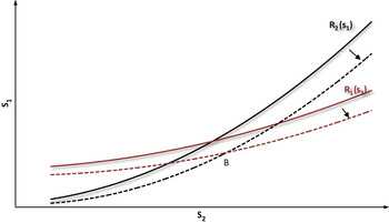
In the appendix we show that the conditions c ′′(s 1) > (∂h/s 1) and c ′′(s 2) > (∂h/s 2) ensure that the second-order conditions for profit maximization hold and the equilibrium is stable. It can also be checked from (5) and (6), and using Lemma 1 that the two reaction functions in cleanup levels are positively sloped, i.e., the first-stage marginal profit of each firm is increasing in the cleanup level of the other firm. Thus the cleanup levels chosen by the firms are strategic complements. Also the reaction function of firm 2 is steeper than that of firm 1. This gives us a unique equilibrium. The reaction functions and their point of intersection are shown in figure 1. R 1(s 2) and R 2(s 1) represent the reaction functions of firms 1 and 2, respectively.
Shift in firms' reaction functions in cleanup levels. With an increase in b, both reaction functions shift to the right moving the equilibrium in cleanup levels from A to B. As compared to A, at B the cleanup level of the cleaner firm, s 2, is higher and that of the inferior firm, s 1, is lower.

Using A.3, the aggregate consumer surplus can be obtained as follows
 $$CS =\int_{a}^{\hat{\theta}}\lpar v+\theta s_{1}-p_{1}\rpar d\!F\lpar \theta \rpar +\int_{\hat{ \theta}}^{b}\lpar v+\theta s_{2}-p_{2}\rpar d\!F\lpar \theta \rpar $$
 $$=\displaystyle{{\lpar \hat{\theta}-a\rpar } \over {\lpar b-a\rpar }}\Bigg[v+\displaystyle{{s_{1}} \over {2}}\lpar \hat{\theta} +a\rpar -p_{1}\Bigg]+\displaystyle{{\lpar b-\hat{\theta}\rpar } \over {\lpar b-a\rpar }}\bigg[v+\displaystyle{{s_{2}} \over {2}}\lpar \hat{ \theta}+b\rpar -p_{2}\bigg]$$
While the first term on the right-hand side of (8) represents consumer surplus enjoyed by the consumers of the lower quality product, the second term represents consumer surplus enjoyed by the consumers of the higher quality product.
We will now characterize economic growth and inequality in income distribution in our setup. Using A.2, the aggregate income in the economy is given by
 $$\eqalign{Y & =\int_{\underline{y}}^{\overline{y}}yt\lpar y\rpar dy \cr & =\displaystyle{{\lpar \underline{y}+\overline{y}\rpar } \over {2}}.}$$
It is evident from the above equation that, for a given size of the population, economic growth can take place via an increase in net
 $\lpar \underline{y}+\overline{y}\rpar $
, that is, with an increase in either y or
 $\overline{y}$
or both, or changes in support of the distribution such that the rise in one is larger than the fall in the other. For modeling economic growth, we are restricting to distributional changes such that the new distribution continues to be uniform and only its support changes.Footnote
2
For simplification, we focus on changes in income distribution such that the new distribution dominates the original distribution in the sense of first-order stochastic dominance. In other words, we allow for y and
 $ \overline{y}$
to rise but not decline.
Variance of the income distribution is
 $$V\lpar y\rpar =\displaystyle{{1} \over {12}}\lpar \overline{y}-\underline{y}\rpar ^{2}.$$
It can trivially be noted that the variance increases with an increase in
 $\overline{y}$
and decreases with an increase in y.
One of the principal inequality measures used widely in economics is the Gini coefficient. It is a number between 0 and 1, with higher values corresponding to greater income inequality. For a continuous income distribution, T(y), the Gini coefficient can be calculated as
 $$G=1-\displaystyle{{1} \over {\mu }}\int_{0}^{\infty }\lpar 1-T\lpar y\rpar \rpar ^{2}dy$$
where μ is the mean of the income distribution (Dorfman, Reference Dorfman1979).
Lemma 2.
Assume distributional changes such that the income distribution remains uniform, and only its support changes. Income inequality (as measured by the Gini coefficient) increases with an increase in
 $\overline{y}$
keeping
y
constant, and decreases with an increase in
y
with
 $\overline{y}$
constant.
Proof: See the appendix.□
It can also be checked that with an increase in
 $\overline{y}$
, the curvature of the Lorenz curve increases, and it decreases with an increase in y. So with a rise in y (with
 $\overline{y}$
fixed), the Lorenz curve for the new distribution would lie wholly above the initial Lorenz curve indicating a decrease in income inequality.
In the next section we study how economic growth changes equilibrium qualities.
3. Comparative statics
In our setup, economic growth takes place via an increase in either
 $\overline{y}$
or y or both. From Lemma 2, the inequality in income distribution increases when
 $\overline{y}$
increases, and decreases when y increases. Given the monotonic relationship between y and θ, a change in the distribution of y changes the distribution of θ.
To gain insights into how changes in the support of the distribution of θ change optimal qualities chosen by the firms, we first examine the effects of changes in a or b on the reaction functions of the two firms.
Lemma 3.
(i) With an increase in b, the reaction functions of both firms shift to the right.
(ii) With an increase in a, the reaction functions of both firms shift to the left.
Proof: See the appendix.□
The shift in the reaction functions due to an increase in b is illustrated in figure 1. With an increase in b the marginal benefit of cleanup increases for firm 2. This induces firm 2 to choose a higher cleanup level for each cleanup level chosen by firm 1. Hence, the reaction function of firm 2, R 2(s 1), shifts to the right. Since the marginal benefit of cleanup for firm 1 decreases, it is induced to choose a lower cleanup level for each given level of cleanup chosen by firm 2, and hence, the reaction function of firm 1, R 1(s 2) also shifts to the right. The point of intersection moves from A to B. At the new intersection point, the cleanup level of firm 2 is unambiguously higher, while that of firm 1 is lower. Similar effects work when a increases; the reaction functions of both firms shift to the left.
We can now investigate the effect of economic growth on the quality choices of two firms.
Proposition 1.
Assume interior solutions and A.1–A.4. An increase in income at the upper end of the income distribution,
 $\overline{y}$
(keeping the lower end constant).
-
(i) unambiguously increases the quality chosen by the environmentally superior firm;
-
(ii) has an ambiguous impact on the quality of the environmentally inferior firm;
-
(iii) lowers the environmental quality of the environmentally inferior firm for 2c ′′(s 2) > 3(∂h/∂s 2).
Proof: See the appendix.□
Since the willingness to pay at the upper end of the income distribution has increased, the cleaner firm improves the quality supplied, and increases its profit by charging a higher price. Its lower end consumers now enjoy a lower surplus than before as the increase in their willingness to pay is less than that of the upper end consumers. The lower quality firm faces a situation where its competitor has differentiated away from it but the willingness to pay of the lower end consumers has not increased. It can lower its quality, and extract greater surplus from the marginal consumers at the upper end. By doing so, it will not lose demand as these consumers cannot move to the cleaner firm. This is because it is more expensive now and their willingness to pay has not increased proportionately. This way the firm is able to retain its demand even by lowering its quality.
Proposition 1 shows that economic growth may not improve quality provision for all the consumers. When economic growth is coupled with increased income inequality, the quality of the variant consumed by high-end consumers improves but the quality consumed by the low-income consumers may deteriorate. Trivially, the gap between the two qualities would rise. Assuming a cost function that is quadratic in quality and linear in quantity, Cremer and Thisse (Reference Cremer and Thisse1994) show that in a duopolistic market equilibrium, firms differentiate their products more than the socially optimal level.Footnote 3 An increase in income inequality would further increase the quality gap between two products, which could have an adverse effect on the welfare of the poor consumers. The condition 2c ′′(s i ) > 3(∂h/∂s i ), i = 1,2 holds for quadratic cost functions and also for more convex cost functions. Thus the result that an increase in income inequality deteriorates the quality choice of the inferior firm holds for a large class of cost functions that are sufficiently convex.
The deterioration in the lower quality product may have serious implications for the consumers at the lower end of the income distribution, especially if the product has a direct health or safety hazard for the user. Despite being aware of these hazards, the consumers at the lower end of the income distribution are forced to consume these products for two reasons. First, the good under consideration is an essential good, and therefore, consumers cannot do without it. Second, the better variant of the product has become more expensive (due to improvement in its quality) and poor consumers cannot afford it at that price.
Proposition 2.
Assume interior solutions and A.1–A.4. An increase in income at the lower end of the income distribution, y (keeping the upper end constant).
-
(i) unambiguously increases the quality chosen by the environmentally inferior firm;
-
(ii) has an ambiguous impact on the quality of the environmentally superior firm;
-
(iii) reduces the environmental quality of the environmentally superior firm for 2c ′′(s 1) > 3(∂h/∂s 1).
Proof: See the appendix.□
Proposition 2 shows that, if economic growth is accompanied by a reduction in income inequality, the quality consumed by the lower end consumers improves, while that consumed by the upper end consumers may fall. Thereby, the gap between the two qualities would also reduce, having a welfare-improving effect. Again the result holds for a large class of sufficiently convex cost functions.
Often developing countries are not applauded for the improved quality of the better products but are blamed for the existence of fringes of heavily polluted products. Rapidly industrializing countries in South-East Asia and Latin America are experiencing pollution ills. Our results suggest that such a situation could be an outcome of increased disparities in income distribution.
The result of deterioration in the cleanup level of lower quality products may cause concern for the planner. The question then arises of whether a government can prevent deterioration in the quality of the inferior product and save its population from such hazardous exposure.
Since the cleanup levels are strategic complements, imposing a cleanup standard exceeding the lowest cleanup level produced in the economy improves the environmental quality of both variants of the product. Consider an economy which is in the process of economic growth. We will restrict ourselves to the economies that are characterized by undercleaning in the absence of market intervention. Let the government impose a standard
 $\hat{s} =s_{1}^{\ast }$
, where superscript * denotes the equilibrium value of the variable in the economy before it experiences economic growth. Observe that as of now, this standard is not binding as it does not affect the equilibrium choice of cleanup levels. The imposed standard assumes significance when the economy experiences economic growth, which increases the willingness to pay for the cleaner product. In the initial period, i.e., the intermediate phase, the growth is likely to be accompanied by increased inequality in income distribution. Proposition 1(iii) tells us that the lower quality firm has an incentive to reduce the cleanup level. The standard now becomes binding for it and prevents the firm from lowering the adopted cleanup level. In the intermediate phase, the standard
 $\lpar \hat{s}\geq s_{1}^{\ast }\rpar $
on cleanup levels prevents the lower quality firm from reducing its quality; at the same time, the higher quality firm improves its quality. As will be shown later in Proposition 3, the standard would again become ineffective, when the growth in income percolates down to the consumer with the least income. An interesting application of our results is in the formulation of bio-safety laws for transgenic crops. Our results support strict bio-safety standards before the approval of transgenic crops for commercial cultivation.
Assuming costless quality, and a trapezoid distribution of income, Benassi et al. (Reference Benassi, Church and Colombo2006) find that a more concentrated income distribution implies stronger product differentiation as the presence of a large share of middle-income consumers stimulates a price competition whose effects are dampened through an enlargement of the quality spread. Yurko (Reference Yurko2011) studies the effects of changes in the consumers' income distribution on the firms' entry decisions and the optimal choices of product attributes and prices assuming a lognormal income distribution, and reaches a similar conclusion. The paper analyzes the case of costless quality and also the case where cost of quality improvement is a fixed cost and finds that a low degree of heterogeneity in consumer incomes intensifies price competition. In order to soften it, firms differentiate their products more when income inequality is lower.
In contrast to the above two papers, we find that an increase in income inequality results in greater product differentiation. Intuitively, the difference in the results can be explained as follows. The cleanup costs in our model are variable costs increasing in the volume of output. When improving quality is costless, product differentiation is an outcome of purely demand-driven strategic behavior. Technology does not act as a constraint in the choice of quality. In a fixed-cost model, quality determines prices only indirectly through shifts in demand. Variable costs, therefore, do not rise ‘too quickly’ with quality. When the cost of cleaning is increasing in both quality and quantity, the quality determines prices directly through cost as well as through shifts in demand. Prices, therefore, rise or fall faster with a change in quality. Variable costs act as technological constraint on the firms' incentives to soften price competition through product differentiation. Further, we have analyzed a duopoly, whereas Yurko (Reference Yurko2011) examines change in qualities through a change in market structure. In section 5, we examine the generalizability of our results when entry is allowed.
4. Specific cost function
In this section we show additional results assuming that the cost function takes a quadratic functional form. We also introduce some new notations that will be used in the remaining sections. To take care of economies with varying distributions of income, we index the economy by the support of the distribution of θ. The distribution of θ changes with a change in the underlying distribution of income. Consider the ordered pair (m,n),m,n ≥ 0. We define an economy E(m, n) as one where the distribution of the willingness to pay, θ, has the support [a + m, b + n]. Observe that, if m = n = 0, we have the original economy before the growth in income. We will compare the E(0, 0) economy with two particular types of E(m, n) economy. The economy characterized by m ≠ n,m,n ≥ 0 can be distinguished from the E(0, 0) economy as one in which the amount of increase in income differs across consumers. In the economy with m = n > 0, each consumer's income is higher than the income of the corresponding consumer in the E(0, 0) economy by the same amount. We state the modified assumptions below. A.5 specifies the functional form of the cost function, A.6 assumes that the new distribution is uniform, and A.7 ensures that both firms enjoy a positive market share in the E(m, n) economy.
-
A.5: C(s,q) = qc(s), where c(s) = ks 2/2, k > 0.
-
A.6: θ is distributed uniformly over [a + m, b + n].
-
A.7: 5(a + m) ≥ (b + n)
Plugging the above-specified functional form into equations (5) and (6), we can obtain closed-form expression of various variables in equilibrium in the E(m, n) economy.
-
(a) The cleanup levels are given by
(9)
$$s_{2} =\displaystyle{{\lpar 5b-a\rpar } \over {4k}}+ \displaystyle{{\lpar 5n-m\rpar } \over {4k}}$$
(10)
$$s_{1} =\displaystyle{{\lpar 5a-b\rpar } \over {4k}} +\displaystyle{{\lpar 5m-n\rpar } \over {4k}}.$$
-
(b) The degree of differentiation, given by the gap between the two variants, is
$$s_{2}-s_{1}=\displaystyle{{3\lpar b-a\rpar } \over {2k}} +\displaystyle {{3\lpar n-m\rpar } \over {2k}}.$$
-
(c) Recall that
$\hat{\theta}$
segregates the consumers between two qualities.
The demand faced by each firm
$$\hat{\theta}=\displaystyle{{\lpar b+a\rpar } \over {2}}+\displaystyle{{\lpar m+n\rpar } \over {2}}$$
$$q_{1}=q_{2}=1/2$$
-
(d) Prices charged by the two firms are
$$\eqalign{& p_{2} =\displaystyle{{1} \over {32k}}[ 49\lpar b+n\rpar ^{2}+25\lpar a+m\rpar ^{2}-58\lpar b+n\rpar \lpar a+m\rpar ] \cr & p_{1} =\displaystyle{{1} \over {32k}}[ 25\lpar b+n\rpar ^{2}+49\lpar a+m\rpar ^{2}-58\lpar b+n\rpar \lpar a+m\rpar ] .}$$
-
(e) Using the demand, price and cost expressions, the profits obtained by the two firms are
(11)
$$\Pi _{1}=\Pi _{2}=\displaystyle{{3} \over {8k}}\lpar b-a+n-m\rpar ^{2}.$$
-
(f) Again using the demand and price expressions in (8), the consumer surplus is given by
(12)
$$\eqalign{CS &=\displaystyle{{1} \over {64k}}[ 62\lpar a+m\rpar \lpar b+n\rpar -19\lpar a+m\rpar ^{2}-27\lpar b+n\rpar ^{2}] \cr & \quad + \displaystyle {{1} \over {64k}}[ 62\lpar a+m\rpar \lpar b+n\rpar -27\lpar a+m\rpar ^{2}-19\lpar b+n\rpar ^{2}] }$$
(13)Proposition 3 compares the E(0, 0) economy with an E(m, n) economy where m = n = r > 0. For each level of θ in E(0, 0), the corresponding person in E(r, r) has a higher income and a higher utility of θ + r per unit of environmental quality.
$$\quad \quad =\displaystyle{{1} \over {32k}}[ 62\lpar a+m\rpar \lpar b+n\rpar -23\lpar a+m\rpar ^{2}-23\lpar b+n\rpar ^{2}] .$$


Proposition 3.
Assume A.4 - A.7, m = n = r > 0, and interior solutions. Compared to the E(0, 0) economy, in E(r, r).
-
(i) both firms have higher cleanup efforts and, hence, total pollution is less;
-
(ii) the gap between the two qualities, measured by the difference s 2 − s 1, is the same;
-
(iii) the proportion of consumers served by each firm is the same;
-
(iv) the profits of both firms are the same;
-
(v) the aggregate consumer surplus as well as consumer surplus enjoyed by each of the groups, low-quality consumers and high-quality consumers, is higher.
Proof: See the appendix.□
When each consumer's income rises uniformly, firms respond to this by improving the quality as well as increasing the price of both variants of the good. The price–quality pairs alter in such a manner that both firms obtain the same profit as before. Proposition 3 tells us that the E(r, r) economy will be more environment friendly than the E(0, 0) economy. It also tells us that firms are equally well off in both economies (Proposition 3(iv)). The consumer surplus enjoyed by both the consumer groups, consumers of the high-quality product as well as consumers of the low-quality product, increases, resulting in an increase in aggregate consumer surplus.
Proposition 4 compares the E(0, 0) economy with an E(m, n) economy where m = 0 < n = r. The growth in income is accompanied by increased inequality in income distribution.
Proposition 4.
Assume A.4–A.7, m = 0 < n = r, and interior solutions. Compared to the E(0, 0) economy, in E(0, r).
-
(i) the cleanup effort of the better quality firm is higher and that of the worse quality firm is lower; however, total pollution is lower;
-
(ii) the gap between the two qualities is higher;
-
(iii) the proportion of consumers served by each firm is the same;
-
(iv) the profit of both firms is higher;
-
(v) the consumer surplus enjoyed by the consumers of cleaner product may go up, and the consumer surplus enjoyed by lower quality product may go down;
-
(vi) the aggregate consumer surplus may be lower.
Proof: See the appendix.□
When economic growth takes a form where income levels of the consumers at the upper end of the income distribution are higher than before, the price and quality pairs adjust in such a manner that both firms enjoy a higher profit. Further, the consumer surplus enjoyed by the high-quality consumers rises and that of the low-quality consumers may fall.
Finally we can analyze the effect of income growth that is accompanied by reduced disparities in income. More specifically, we consider an increase in income such that 0 < n < m. From (9)–(11) we know that such a rise in income may reduce cleanup of the high-quality firm, improves the cleanup of the low-quality firm, improves overall environmental quality, and reduces the degree of differentiation between the two variants of the products. It is easy to see that with a growth in income of (n < m) type, profits of both firms are reduced.
5. Market structure
Assuming a uniform income distribution, costless quality and imposing the condition b < 4a, where [a, b] are the supports of the income distribution, Shaked and Sutton (Reference Shaked and Sutton1982) show that there is an upper bound on the number of firms with positive market shares. We now generalize the finiteness property of Shaked and Sutton to the case where costs of production are positive, and the utility function is quasilinear.
Suppose that there are n potential firms each producing a distinct variant. Let p i and s i , respectively, be the price and the quality of variant i, (i = 1, …, n). Also let products be labeled in increasing order of quality s 1 < s 2 < s 3… < s n . We show that the finiteness property holds if costs of production are not rising too fast in quality, more specifically, if the equilibrium quantities and prices are such that
 $$p_{i-1}^{\ast }-c\lpar s_{i}^{\ast }\rpar \geq 0 \quad for \, \, all \quad i.$$
Proposition 5.
Let b < 4a. Assume A.1–A.3 and equilibrium prices and qualities are such that p i−1* − c(s i *) ≥ 0 for all i. Then for any Nash equilibrium involving the distinct goods, at most two firms can have positive market share at equilibrium.
Proof: See the appendix.□
Proposition 5 shows that the results obtained in the paper would hold even when entry is allowed as long as the gap between the consumer with the highest income and the one with the lowest income is not too large and the costs of improving quality are not rising too sharply.
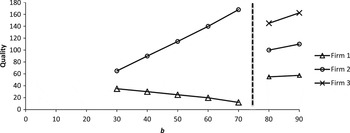
We now relax the above restrictions, and check the number of firms with positive market share when entry is allowed. Following Yurko (Reference Yurko2011), we numerically compute the equilibrium number of firms, the qualities and prices in a market outcome. Consider a three-stage model, where firms decide whether or not to enter in the first stage, choose qualities in the second stage and compete in prices in the third stage. Assume A.4–A.6, and k = 1. The outputs of the model are number of firms, product qualities and product price, and the major input is the support of the distribution of the willingness to pay parameter, θ. Observe that an entry stage has been added to the model developed in section 2. The model is solved using R software. The code is available in an online Appendix available at http://journals.cambridge.org/EDE.Footnote 4 We find that only two firms exist with positive market share as the support of the distribution of θ changes from [20, 30] to [20, 70]; however, as the upper end of the support, b, increases beyond 80, the number of firms with positive market share increases to three. Figure 2 graphically illustrates the equilibrium qualities of firms as a function of b. The lower end, a, has been kept at 20. It can be seen that for 30 ≤ b < 80, the number of firms with positive market share is two, and clearly the quality gap between the two firms is increasing with an increase in income inequality. However, for 80 ≤ b < 100, the number of firms with positive market share becomes three and we cannot say the same for the trend in the quality gap.
Equilibrium qualities as a function of the upper end of the support of the distribution of marginal willingness to pay parameter, b, where a has been fixed at 20. The number of firms with positive market share is two for 30 ≤ b < 80, and is three for 80 ≤ b < 100.

6. Conclusion
In this paper, we examine the effect of economic growth on the cleanup activity of firms in an economy where consumers are environmentally aware and are willing to pay a price premium for environmentally superior qualities. The growth in income may take different forms. When income of all the consumers increases by the same amount, cleanup levels rise for both firms, resulting in improved environmental quality. When the increase in income differs across consumers, both qualities may not improve. In particular, if the increase in income is coupled with an increase in the disparities in the income distribution, the quality of the inferior product is adversely affected. This has serious implications for poor consumers. They are now forced to buy a quality which is even lower than the one they were buying before. This causes concern for the government. It is indeed often observed that growth concerns in developing countries center almost exclusively on the upper socio-economic echelon of society. These economies are characterized by the presence of elite premium quality products accessible to the high-end consumers co-existing with very low qualities for the lower end consumers.
One of the ways to prevent deterioration in quality is to impose a cleanup standard equal to the quality of the inferior product. Such a standard is ineffective at the current levels of income. If there is growth in income without any change in inequality in income distribution, this standard continues to be ineffective. However, if the growth in income takes a form where the inferior quality firm has an incentive to reduce the quality further, the imposed standard prevents it from doing so.
An alternative way of changing the distribution of marginal willingness to pay for environmental quality is through changing consumer awareness. The government and non-governmental organizations through information and peer pressure are making efforts to raise the awareness of the harmful effects of pollution. The decision of consumers regarding the quality of the product is determined also by their knowledge of the environmental bad. If a poor household is aware of the health hazard to children of smoke-filled homes, it will be more inclined to move towards cleaner fuels (to kerosene from firewood) even if it cannot afford the cleanest fuel (cooking gas or electricity). The effects of an increase in the degree of environmental awareness among consumers are similar to the effects of increased incomes. Our results suggest that these awareness campaigns should be carefully designed. If they target only the richer sections of the society, they could lead to deterioration in the quality consumed by the poorer consumers. It may be a better policy to first target poorer households for the awareness campaigns.
The analysis in the paper has assumed a duopoly competition with no entry or exit. For checking robustness of the results we also examine how allowing free entry and exit affects our results. We find that, as long as the inequality in income distribution is not very large, our results hold even under free entry and exit. However, when the inequality in income distribution becomes sufficiently large, more firms may be induced to enter, altering our results.
Appendix
Second-order sufficient conditions for profit maximization and stability of the equilibrium
Using the definition of h (from Lemma 1) in (5) and (6) and assuming c ′′(s i ) > (∂h/s i ), i = 1,2, it can be checked that
 $$\displaystyle{{\partial ^{2}\pi _{1}} \over {\partial s_{1}^{2}}} = \displaystyle{{\partial h} \over { \partial s_{1}}}-2c^{\prime \prime }\lpar s_{1}\rpar \lt 0$$
 $$\displaystyle{{\partial ^{2}\pi _{2}} \over {\partial s_{2}^{2}}} = \displaystyle{{\partial h} \over { \partial s_{2}}}-2c^{\prime \prime }\lpar s_{2}\rpar \lt 0.$$
Thus the second-order sufficient conditions for profit maximization are satisfied. It can also be checked that the equilibrium is stable.
 $$\eqalign{\displaystyle{{\partial ^{2}\pi _{1}} \over {\partial s_{1}^{2}}} \displaystyle{{\partial ^{2}\pi _{2}} \over {\partial s_{2}^{2}}}-\displaystyle{{\partial \pi _{1}^{2}} \over {\partial s_{1}\partial s_{2} }} \displaystyle{{\partial \pi _{2}^{2}} \over {\partial s_{1}\partial s_{2}}} & =c^{\prime \prime }\lpar s_{1}\rpar \left[c^{\prime \prime }\lpar s_{2}\rpar -\displaystyle{{\partial h} \over{\partial s_{2}}}\right]\cr & +c^{\prime \prime }\lpar s_{2}\rpar \left[c^{\prime \prime }\lpar s_{1}\rpar -\displaystyle{{\partial h} \over { \partial s_{1}}}\right]\geq 0}$$
Proof of Lemma 2
Using A.2, the Gini coefficient for the uniform distribution considered in the paper is
 $$\eqalign{G &= 1-\displaystyle{{1} \over {\mu }}\bigg[\int_{0}^{\underline{y}}\lpar 1-H\lpar y\rpar \rpar ^{2}dy+\int_{ \underline{y}}^{\overline{y}}\lpar 1-H\lpar y\rpar \rpar ^{2}dy+\int_{\overline{y}}^{\infty }\lpar 1-H\lpar y\rpar \rpar ^{2}dy\bigg]\cr &= 1-\displaystyle{{2} \over {\lpar \underline{y}+\overline{y}\rpar }}\bigg[\underline{y}+\int_{ \underline{y}}^{\overline{y}}\lpar \displaystyle{{\overline{y}-y} \over {\overline{y}-\underline{y }}}\rpar ^{2}dy+0\bigg]\cr &= 1-\displaystyle{{2} \over {\lpar \underline{y}+\overline{y}\rpar }}[ \underline{y}+\displaystyle{{\overline{y}- \underline{y}} \over {3}}] \cr &= \displaystyle{{\lpar \overline{y}-\underline{y}\rpar } \over {3\lpar \overline{y}+\underline{y}\rpar }}.}$$
It can be checked that
 $\partial G/\partial \overline{y}>0$
, and
 $\partial G/\partial \underline{y}<0$
.
Proof of Lemma 3
Taking a partial derivative of equation (5) with respect to b taking a and s 1 as given,
 $$\displaystyle{{\partial s_{2}} \over {\partial b}}=\displaystyle{{2} \over {2c^{\prime \prime }\lpar s_{2}\rpar -\displaystyle{{ \partial h} \over {\partial s_{2}}}}} \gt 0 \quad \quad for\, \, all \quad s_{1}.$$
Again taking a partial derivative of (6) with respect to b taking a and s 2 as given,
 $$\displaystyle{{\partial s_{1}} \over {\partial b}}=\displaystyle{{-1} \over {2c^{\prime \prime }\lpar s_{1}\rpar -\displaystyle{{ \partial h} \over {\partial s_{1}}}}} \lt 0 \quad \quad for\, \, all \quad s_{2}.$$
Since the denominators are positive from the second-order conditions, the sign of the derivative is determined by the sign of the numerator. (∂s 2/∂b) > 0 for all s 1 implies that the reaction function of firm 2 shifts to the right with a rise in b. And (∂s 1/∂b) < 0 for all s 2 implies that the reaction function of firm 1 also shifts to the right with a rise in b.
Similarly partially differentiating equations (5) and (6) with respect to a, it can be checked that
 $$\displaystyle{{\partial s_{2}} \over {\partial a}} = \displaystyle{{-1} \over {2c^{\prime \prime }\lpar s_{2}\rpar -\displaystyle{{ \partial h} \over {\partial s_{2}}}}} \lt 0 \quad \quad for\, \, all \quad s_{1}$$
 $$\displaystyle{{\partial s_{1}} \over {\partial a}}=\displaystyle{{2} \over {2c^{\prime \prime }\lpar s_{1}\rpar -\displaystyle{{ \partial h} \over {\partial s_{1}}}}} \gt 0 \quad \quad for\, \, all \quad s_{2}.$$
The direction of the shift of the reaction functions follows.
Proof of Proposition 1
Totally differentiating equations (5) and (6), we obtain the following matrix
 $$\left({\matrix{ {2c^{\prime \prime}\lpar {s_2}\rpar - \displaystyle{{\partial h} \over {\partial {s_2}}}} & { - \displaystyle{{\partial h} \over {\partial {s_1}}}} \cr { - \displaystyle{{\partial h} \over {\partial {s_2}}}} & {2c^{\prime \prime}\lpar {s_1}\rpar - \displaystyle{{\partial h} \over {\partial {s_1}}}} \cr } } \right)\left({\matrix{ {d{s_2}} \cr {d{s_1}} \cr } } \right)= \left({\matrix{ 2 & { - 1} \cr { - 1} & 2 \cr } } \right)\left({\matrix{ {db} \cr {da} \cr } } \right).$$
It can be checked that
 $$sign \displaystyle{{ds_{2}} \over {d\overline{y}}}= sign \displaystyle{{ds_{2}} \over {db}} = sign \left[4c^{\prime \prime }\lpar s_{1}\rpar -3 \displaystyle{{\partial h} \over {\partial s_{1}}}\right] \gt 0.$$
The first equality follows from the monotonic relationship between θ and y, the second equality follows from equation (15), and the inequality follows from the second-order conditions. Similarly
 $$\eqalign{sign \displaystyle{{ds_{1}} \over {d\overline{y}}} &= sign \displaystyle{{ds_{1}} \over {db}} = sign \left[-2c^{\prime \prime }\lpar s_{2}\rpar +3\displaystyle{{\partial h} \over {\partial s_{2}}}\right] \lt 0 \cr & \quad for \quad 2c^{\prime \prime }\lpar s_{2}\rpar \gt 3 \displaystyle{{\partial h} \over {\partial s_{2}}}.}$$
Proof of Proposition 2
Again from (15), it can be checked that
 $$sign \displaystyle{{ds_{1}} \over {d\underline{y}}} = sign \displaystyle{{ds_{1}} \over {da}} = sign \left[4c^{\prime \prime }\lpar s_{2}\rpar -3\displaystyle{{\partial h} \over {\partial s_{2}}}\right] \gt 0 $$
 $$\eqalign{sign \displaystyle{{ds_{2}} \over {d\underline{y}}} & = sign \displaystyle{{ds_{2}} \over {da}} = sign \left[-2c^{\prime \prime }\lpar s_{1}\rpar +3 \displaystyle{{\partial h} \over {\partial s_{1}}}\right] \lt 0 \cr & \quad for \quad 2c^{\prime \prime }\lpar s_{1}\rpar \gt 3\displaystyle{{\partial h} \over {\partial s_{1}}}.}$$
Proof of Proposition 3
Let superscripts * and~ denote the equilibrium value of the variables for the E(0, 0) and E(r, r) economy, respectively. Plugging m = n = r > 0 into (a)–(f) in section 4, it is straightforward to see
-
(i) The cleanup levels
$$\eqalign{& \tilde{s_1} = s_1^{\ast} +\displaystyle{{r} \over {k}} \cr & \tilde{s_2} = s_2^{\ast} + \displaystyle{{r} \over {k}}}$$
-
(ii) The degree of differentiation
$$\tilde{s_2}-\tilde{s_1}= s_2^{\ast}-s_1^{\ast}$$
-
(iii) The demand faced by each firm
$$\tilde{q_1}=\tilde{q_2}=q_i^{\ast}\comma \; i=1\comma \; 2$$
The prices charged by the two firms are
$$\eqalign{& \tilde{p_{2}} = p_{2}^{\ast }+\displaystyle{{r^{2}} \over {2k}}+\displaystyle{{r\lpar 5b-a\rpar } \over {4k}} \cr & \tilde{p_{1}} = p_{1}^{\ast }+\displaystyle{{r} \over {2k}}+\displaystyle{{r\lpar 5a-b\rpar } \over {4k}}}$$
-
(iv) The profit obtained by the two firms are
$$\tilde{\Pi_1}=\tilde{\Pi_2}=\displaystyle{{3\lpar b-a\rpar ^2} \over {8k}}=\Pi^{\ast}_i\comma \; i=1\comma \; 2$$
and
-
(v) The consumer surplus enjoyed by consumers
(19)
$$\eqalign{\tilde{CS} &= \displaystyle{{1} \over {64k}}[ 62\lpar a+r\rpar \lpar b+r\rpar -19\lpar a+r\rpar ^{2}-27\lpar b+r\rpar ^{2}] \cr & + \displaystyle{{1} \over {64k}}[ 62\lpar a+r\rpar \lpar b+r\rpar -27\lpar a+r\rpar ^{2}-19\lpar b+r\rpar ^{2}] }$$
(20)
$$\quad = \displaystyle{{1} \over {32k}} [62\lpar a+r\rpar \lpar b+r\rpar -23\lpar a+r\rpar ^{2}-23\lpar b+r\rpar ^{2}] .$$
While the first term in the right hand side of (19) is the consumer surplus enjoyed by the consumers of the lower quality product (C~S 1), the second term is the consumer surplus enjoyed by the consumers of the higher quality (C~S 2).
$$\displaystyle{{\partial \tilde{CS_{1}}} \over {\partial r}} =\displaystyle{{1} \over {8}} [3\lpar a+r\rpar +\lpar b+r\rpar ] \gt 0$$
$$\displaystyle{{\partial \tilde{CS_{2}}} \over {\partial r}} = \displaystyle{{1} \over {8}}[ \lpar a+r\rpar +3\lpar b+r\rpar ] \gt 0$$
$$\displaystyle{{\partial \tilde{CS}} \over {\partial r}} =\displaystyle{{1} \over {2}} \lpar a+b+2r\rpar \gt 0$$


Proof of Proposition 4
The proof follows from plugging m = 0, n = r > 0 into (a)–(f) in section 4. Let a superscript ′ denote the value of the variables in equilibrium in E(0, r) economy.
-
(i) The cleanup levels
$$\eqalign{& s^{\prime }_2 =s^{\ast}_2 + \displaystyle{{5r} \over {4k}} \cr & s^{\prime }_1 = s_1^{\ast}-\displaystyle{{r} \over {4k}}}$$
-
(ii) The degree of differentiation
$$s^{\prime }_2 -s^{\prime }_1= s_2^{\ast}-s_1^{\ast}+\displaystyle{{3r} \over {2k}}$$
-
(iii) The demand faced by each firm
$$q^{\prime }_1=q^{\prime }_2=1/2$$
Prices charged by the two firms are
$$\eqalign{& p^{\prime }_2 = p_1^{\ast} + \displaystyle{{49r^2} \over {32k}} + \displaystyle{{r\lpar 49b-29a\rpar } \over {16k}} \gt p_2^{\ast} \cr & p^{\prime }_1 = p_2^{\ast}+ \displaystyle{{25r^2} \over {32k}} +\displaystyle{{r\lpar 25b-29a\rpar } \over {16k}} \cr & \displaystyle{{\partial p^{\prime }_1} \over {\partial r}}= \displaystyle{{1} \over {32k}}\lpar 50 \lpar b+r\rpar -58a\rpar {\geqq \over \lt} 0 \quad as \quad [25\lpar b+r\rpar /29] {\geqq \over \lt} a}$$
-
(iv) The profit obtained by each firm
$$\Pi_{1}^{\prime }=\Pi_{2}^{\prime }=\displaystyle{{3} \over {8k}} \lpar b+r-a\rpar ^2 \gt \Pi_i^{\ast}\comma \; i=1\comma \; 2$$
-
(v) Consumer surplus enjoyed by consumers of each quality
$$\eqalign{& \displaystyle{{\partial CS^{\prime }_2} \over {\partial r}} =\displaystyle{{1} \over {32k}}\lpar 31a-19\lpar b+r\rpar >0 \quad for \quad a > \lpar 19/31\rpar \lpar b+r\rpar \cr & \displaystyle{{\partial CS^{\prime }_1} \over {\partial r}} = \displaystyle{{1} \over {32k}} [31a-27\lpar b+r\rpar ] \lt 0 \quad for \quad a<\lpar {27}/{31}\rpar \lpar b+r\rpar }$$
-
(vi) Finally the aggregate consumer surplus may fall
$$\displaystyle{{\partial CS^{\prime }} \over {\partial r}} = \displaystyle{{1} \over {16k}} [31a - 23\lpar b+r\rpar ] \lt 0 \quad for \quad a \lt \lpar 23/31\rpar \lpar b+r\rpar$$


Proof of Proposition 5
The steps of the proof follow Shaked and Sutton (Reference Shaked and Sutton1982). The second-stage profit function of the ith firm is
 $$\pi_i \lpar s\comma \; p\rpar =\lpar p_i-c\lpar s_i\rpar \rpar q_i \lpar s\comma \; p\rpar \comma \; i=1\comma \; 2\comma \; \ldots n$$
 $$\eqalign{\pi_1 & = \lpar p_1-c\lpar s_1\rpar \rpar \displaystyle{{\lpar \theta_2-a\rpar } \over {b-a}}\comma \; \theta_1 \leq a \cr & = \lpar p_1-c\lpar s_1\rpar \rpar \displaystyle{{\lpar \theta_2-\theta_1\rpar } \over {b-a}}\comma \; \theta_1 \geq a \cr & \pi_i = \lpar p_i- c\lpar s_i\rpar \rpar \displaystyle{{\lpar \theta_{i+1}-\theta_i\rpar } \over {b-a}}\comma \; 1 \lt i \lt n \cr & \pi_n = \lpar p_n-c\lpar s_n\rpar \rpar \displaystyle{{\lpar b-\theta_n\rpar } \over {b-a}}}$$
where
 $$\theta_i=\displaystyle{{p_i-p_{i-1}} \over {s_{i}-s_{i-1}}}\comma \; i=2\comma \; ...n\comma \; \theta_1 = \displaystyle{{p_1} \over {s_1}}$$
Let δ i = [1/(s i − s i−1)], i = 2…n Maximizing the second-stage profits with respect to prices, the first-order conditions take the form
 $$\eqalign{& \theta_{i+1} - \theta_i -\lpar p_i-c\lpar s_i\rpar \rpar \lpar \delta_{i+1} + \delta_i\rpar = 0\comma \; \quad i=2\comma \; \ldots n-1 \cr & \quad \quad \quad \quad b-\theta_n-\delta_n\lpar p_n-c\lpar s_n\rpar \rpar = 0}$$
Rewriting the first-order conditions and using the definition of θ i ,
 $$\eqalign{& \theta_{i+1}-2\theta_i -\delta_{i+1}\lpar p_i-c\lpar s_i\rpar \rpar -\delta_i\lpar p_{i-1}-c\lpar s_i\rpar \rpar =0\comma \; i=2\comma \; \ldots\comma \; n-1 \cr & \quad \quad \quad \quad b-2\theta_n-\delta_n\lpar p_{n-1}-c\lpar s_n\rpar \rpar = 0}$$
Since δ i is positive for all i, it follows
 $$\theta_{i+1} - 2\theta_i \geq 0 \quad for \quad p_{i-1} \geq c\lpar s_i\rpar \comma \; i=2\comma \; \ldots\comma \; n-1 $$
 $$b-2\theta_n \geq 0\comma \; \quad for \quad p_{n-1} \gt c\lpar s_n\rpar $$
 $$4\theta_{n-1} \lt b$$
Given the assumption b < 4a, θ n−1 < a; that is, the top two firms cover the market. For the case of costless quality improvement and quasi-linear utility function, the result follows trivially.