2. Evolution equations and numerical simulations

Consider the flow of a dilute polymer solution whose kinematic viscosity has contributions of $\nu$ from the solvent and $\nu _p$ from the polymer. The latter is proportional to the concentration of the polymer, which is characterized by its relaxation time to equilibrium, $\tau _p$, and the squared ratio of its contour length to the equilibrium length, i.e. the extensibility parameter $b$. The dynamics of the solution is then described in terms of the velocity field $\boldsymbol {u}(\boldsymbol {x},t)$ and the polymer conformation tensor $\boldsymbol{\mathsf{C}}(\boldsymbol {x},t)$, here scaled by the mean squared extension at equilibrium. Adopting either the Oldroyd-B or the FENE-P model, and considering the limit of negligible fluid inertia, we obtain the following coupled equations for $\boldsymbol{\mathsf{C}}(\boldsymbol {x},t)$ and $\boldsymbol {u}(\boldsymbol {x},t)$:

(2.1a)$$\begin{gather} \partial_t \boldsymbol{\mathsf{C}} + \boldsymbol{u}\boldsymbol{\cdot}\boldsymbol{\nabla}\boldsymbol{\mathsf{C}} = \boldsymbol{\mathsf{C}}\boldsymbol{\cdot}\boldsymbol{\nabla}\boldsymbol{u} + (\boldsymbol{\nabla}\boldsymbol{u})^{\rm T} \boldsymbol{\cdot}\boldsymbol{\mathsf{C}} -\boldsymbol{\mathsf{T}}_p, \end{gather}$$

(2.1b)$$\begin{gather}\boldsymbol{\nabla} p = \nu\,\Delta\boldsymbol{u} + \nu_p\,\boldsymbol{\nabla}\boldsymbol{\cdot} \boldsymbol{\mathsf{T}}_p + \boldsymbol{F}, \end{gather}$$

(2.1c)$$\begin{gather}\boldsymbol{\nabla}\boldsymbol{\cdot}\boldsymbol{u}=0, \end{gather}$$

where $p$ is the ratio of pressure to the constant density of the solution, $(\boldsymbol {\nabla }\boldsymbol {u})_{ij}=\partial _i u_j$, and $\boldsymbol {F}$ is a body forcing. The polymer contribution to the stress tensor, $\boldsymbol{\mathsf{T}}_p$, takes the form

(2.2)\begin{equation} \boldsymbol{\mathsf{T}}_p=\frac{1}{\tau_p}\,[\,f(r)\,\boldsymbol{\mathsf{C}}-\boldsymbol{\mathsf{I}}], \end{equation}

where $f(r)=1$ for the Oldroyd-B model, and $f(r)=(b-d)/(b-r^2)$ for the FENE-P model. Here, $d$ is the space dimension, $r=\sqrt {\operatorname {tr}\boldsymbol{\mathsf{C}}}$, and $\boldsymbol{\mathsf{I}}$ is the identity matrix.

We have considered the Stokes limit for ease of computation, since we are interested in flows at low Reynolds number ($Re$) for which the chaotic dynamics is driven solely by elastic instabilities. The same approach was taken, for instance, in Thomases & Shelley (Reference Thomases and Shelley2009), Balci et al. (Reference Balci, Thomases, Renardy and Doering2011) and Gutierrez-Castillo et al. (Reference Gutierrez-Castillo, Kagel and Thomases2020). In any case, the difficulties encountered in numerical simulations arise from the advection of the polymer conformation tensor and would be the same if the Navier–Stokes equations (with $Re \lesssim 1$) were used to evolve the flow. In fact, we have repeated some of our key calculations with the Navier–Stokes equations and found that our conclusions remain unchanged (see the supplementary material available at https://doi.org/10.1017/jfm.2024.858).

2.1. Lower bound on the determinant of $\boldsymbol{\mathsf{C}}$

The polymer conformation tensor is positive-definite by construction, hence its determinant must be positive. This property is preserved by (2.1) (Constantin & Kliegl Reference Constantin and Kliegl2012). However, for the Oldroyd-B model, (2.1a) and (2.1c) have stronger implications on the determinant of $\boldsymbol{\mathsf{C}}$: Hu & Lelièvre (Reference Hu and Lelièvre2007) proved that at long times, the determinant of $\boldsymbol{\mathsf{C}}$ must satisfy the bound

(2.3)\begin{equation} \det\boldsymbol{\mathsf{C}}\geq 1 \end{equation}

everywhere in the domain. More precisely, let us denote the value of the conformation tensor along a given Lagrangian trajectory $\boldsymbol {x}_p(t)$ as $\boldsymbol{\mathsf{C}}(t)=\boldsymbol{\mathsf{C}}(\boldsymbol {x}_p(t),t)$. If there exists a time $t_\star$ such that $\det \boldsymbol{\mathsf{C}}(t_\star )\geq 1$, then $\det \boldsymbol{\mathsf{C}}(t)\geq 1$ for all $t > t_\star$. If in contrast $\det \boldsymbol{\mathsf{C}}(t_\star )< 1$, then $\det \boldsymbol{\mathsf{C}}(t)$ keeps growing as long as $\det \boldsymbol{\mathsf{C}}(t)< 1$. When applied to all trajectories, this result implies that, asymptotically in time, (2.3) must hold everywhere in space. Obviously, if at time $t=0$ the determinant of $\boldsymbol{\mathsf{C}}$ is greater than or equal to unity, as is the case in most simulations and certainly in all those presented here, then it must remain so throughout the subsequent evolution.

It is important to note that (2.3) has been proved only for the Oldroyd-B model (Hu & Lelièvre Reference Hu and Lelièvre2007), and a similar result that is local in space and time and uniform in $\boldsymbol {\nabla }\boldsymbol {u}$ is not available, to our knowledge, for the FENE-P model. A bound analogous to (2.3) has been derived, though, for the Giesekus model (Masmoudi Reference Masmoudi2011).

When (2.3) is combined with the inequality $\operatorname {tr}\boldsymbol{\mathsf{C}}\geq d(\det \boldsymbol{\mathsf{C}})^{1/d}$, which holds for any symmetric positive-definite $d\times d$ matrix, we obtain

(2.4)\begin{equation} \operatorname{tr}\boldsymbol{\mathsf{C}}\geq d. \end{equation}

This bound on the trace of $\boldsymbol{\mathsf{C}}$, which was also derived by Musacchio (Reference Musacchio2002) using dynamical systems theory, has a natural physical interpretation. Recall that $\operatorname {tr}\boldsymbol{\mathsf{C}}$ is the squared extension of the polymer, ensemble-averaged over thermal noise, and that $\operatorname {tr}\boldsymbol{\mathsf{C}} = d$ when the polymer solution is at equilibrium (for which $\boldsymbol{\mathsf{C}}=\boldsymbol{\mathsf{I}}$ since $\boldsymbol{\mathsf{C}}$ has been scaled by the mean square polymer extension at equilibrium). Hence (2.4) implies that an incompressible flow cannot squeeze a polymer below its mean equilibrium extension.

We will show below that (2.3) is a useful criterion for testing the accuracy of numerical simulations.

3. Matrix decompositions and erroneous large-scale dynamics

We begin by comparing the results obtained using different decompositions of $\boldsymbol{\mathsf{C}}$. The simulations in this section are devoid of polymer-stress diffusion, i.e. $Pe=\infty$, and use the Oldroyd-B model, which makes the bound (2.3) available for testing the accuracy of the results.

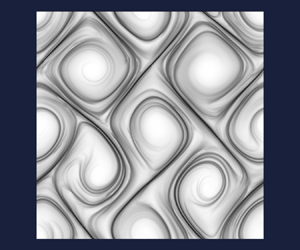
Figures 1(a) and 1(b) compare two representative snapshots of $\operatorname {tr}\boldsymbol{\mathsf{C}}$ (the squared extension of the polymer) for the Cholesky-log and the SSR decompositions (corresponding animations are available in supplementary movie 1). The cellular forcing produces several large vortical cells, wherein the polymer is coiled and $\operatorname {tr}\boldsymbol{\mathsf{C}}$ is small, separated by straining zones that give rise to thin filamentary regions, wherein the polymer is strongly stretched and $\operatorname {tr}\boldsymbol{\mathsf{C}}$ is large. While the vortical cells are perturbed by the chaotic flow, in both simulations, it is clear that the symmetry of the forcing structure is much more closely preserved in the case of the Cholesky-log simulation, as compared to the SSR simulation. The former exhibits a well-ordered lattice of vortical cells, all of which maintain nearly the same orientation and shape throughout the simulation (figure 1a). In contrast, the vortical cells of the SSR simulation constantly change their orientation, shape and size, as from time to time some cells expand while others shrink (figure 1b).

Figure 1.

Representative snapshots (instantaneous) of the logarithm of $\operatorname {tr}\boldsymbol{\mathsf{C}}$ for (a) the Cholesky-log decomposition and (b) the SSR decomposition. For the corresponding animations, see supplementary movie 1. Both simulations use the Oldroyd-B model.

These differences in the large-scale structures of the field of $\operatorname {tr}\boldsymbol{\mathsf{C}}$ are not merely momentary but persist over time, as evidenced by the time-averaged fields presented in figure 2. The plots for the two decompositions are strikingly dissimilar. The time-averaged field for the Cholesky-log simulation closely resembles the corresponding instantaneous field (compare figures 2(a) and 1(a)). The straining zones experience small chaotic oscillations and so are slightly smeared out in the time-averaged plot. In the SSR simulation, the time-averaged field looks very different from its instantaneous snapshot (figures 2(b) and 1(b)); the jostling of the vortical cells produces a time-averaged picture of smeared cells with a high degree of symmetry unseen at any instant of time. Note that this contrast between the large scales of the two simulations also appears in their vorticity fields (as illustrated in the supplementary material), since the variations of vorticity are well correlated with those of $\operatorname {tr}\boldsymbol{\mathsf{C}}$.

Figure 2.

Time-averaged fields of the logarithm of $\operatorname {tr}\boldsymbol{\mathsf{C}}$ for (a) the Cholesky-log decomposition and (b) the SSR decomposition. Both simulations use the Oldroyd-B model.

As a simple measure of the extent to which the cellular structure is perturbed during the evolution, we introduce the diagnostic

(3.1)\begin{equation} \varDelta(t)=\left\lvert\dfrac{\ln[\operatorname{tr}\boldsymbol{\mathsf{C}}((0,0),t)]-\ln[\operatorname{tr}\boldsymbol{\mathsf{C}}(({\rm \pi},0),t)]}{\ln[\operatorname{tr}\boldsymbol{\mathsf{C}}((0,0),t)]+\ln[\operatorname{tr}\boldsymbol{\mathsf{C}}(({\rm \pi},0),t)]}\right\rvert. \end{equation}

This quantity will be zero if the $\operatorname {tr}\boldsymbol{\mathsf{C}}$ field perfectly preserves the cellular structure of the periodic forcing, which has wavenumber $K = 2$. Therefore, $\varDelta$ is indicative of the extent of distortion of the cellular structure, albeit at a single point. The time series of $\varDelta (t)$ is plotted in figure 3(a). Clearly, the fluctuations of $\varDelta (t)$ are significantly stronger for the SSR decomposition than for the Cholesky-log decomposition.

Figure 3.

(a) Time series of $\varDelta$ (defined in (3.1)). (b) Time series of the space averages of $\operatorname {tr}\boldsymbol{\mathsf{C}}$ (main graph) and the kinetic energy $e(t)$ scaled by its Newtonian value $e_0=\frac {1}{2}U^2$ (inset). All plots refer to simulations of the Oldroyd-B model.

The space-averaged statistics of the two simulations are presented in figure 3(b). The main graph compares the mean polymer stretching, given by the spatial average of the trace of the conformation tensor $\langle \operatorname {tr}\boldsymbol{\mathsf{C}} \rangle _{V} = (2{\rm \pi} )^{-2}\int _V \operatorname {tr}\boldsymbol{\mathsf{C}} \, \mathrm {d}\kern0.06em \boldsymbol {x}$, and shows that it is higher for the SSR simulation. This is consistent with the the SSR simulation having a lower mean kinetic energy $e(t)=\frac {1}{2}\langle \boldsymbol {u}\boldsymbol {\cdot }\boldsymbol {u}\rangle _{V}$, as shown in the inset, because higher stretching in the straining zones endows the solution with a higher extensional viscosity (Larson Reference Larson1999). The differences in these mean statistics are rather small in comparison with the differences in the structure and dynamics of the vortical cells, evident from the full fields (figures 1 and 2).

It is important to note that the differences in the predictions of the two decompositions are independent of resolution. We have found that increasing the resolution from $256^2$ to $1024^2$ produces sharper stretching zones in both simulations but no qualitative change in the large-scale dynamics; all the differences discussed above persist.

So which of the two simulations is correct? This question is difficult to address in the present context because, as discussed in the Introduction, elastic turbulence depends on the specific setting and hence lacks universal laws against which numerical predictions may be tested. In the case of the Oldroyd-B model, though, the lower bound $\det \boldsymbol{\mathsf{C}} \geq 1$ presented in § 2.1 comes to our aid. The time series of the minimum of $\det \boldsymbol{\mathsf{C}}$ over the domain is presented in figure 4. We see that the lower bound is respected throughout the Cholesky-log simulation (figure 4a), whereas it is frequently violated in the SSR simulation (figure 4b). While such violations are found to occur over a small fraction of the domain (approximately 0.1 %), they are very frequent in time and very strong – we see many instances where $\det \boldsymbol{\mathsf{C}}$ approaches zero. This leads us to conclude that the SSR simulation is erroneous, and its distinguishing features, including the distortion of the cellular structure, are a consequence of inaccuracies in evolving the polymer stresses.

Figure 4.

Time series of the minimum of $\det \boldsymbol{\mathsf{C}}$ over the domain for (a) the Cholesky-log decomposition, and (b) the SSR decomposition. The bound $\det \boldsymbol{\mathsf{C}} \geq 1$ (see (2.3)) is satisfied by the former simulation but is repeatedly and strongly violated by the latter. The insets show the corresponding time series of $\operatorname {tr}\boldsymbol{\mathsf{C}}$, which as a consequence of (2.3) must remain greater than 2. All plots refer to simulations of the Oldroyd-B model.

In § 2.1, we recalled that the lower bound on $\det \boldsymbol{\mathsf{C}}$ implies a lower bound on the squared extension, $\operatorname {tr}\boldsymbol{\mathsf{C}} \geq 2$. Thus a simulation that respects the bound on $\det \boldsymbol{\mathsf{C}}$ must necessarily respect the bound on $\operatorname {tr}\boldsymbol{\mathsf{C}}$ as well. This is seen in the inset of figure 4(a), which presents the time series of the minimum of $\operatorname {tr}\boldsymbol{\mathsf{C}}$ for the Cholesky-log simulation. In contrast, the SSR simulation violates both bounds (figure 4b), though the instances of $\operatorname {tr}\boldsymbol{\mathsf{C}}$ falling below 2 are much fewer than those of $\det \boldsymbol{\mathsf{C}}$ falling below 1. So while $\operatorname {tr}\boldsymbol{\mathsf{C}}$ has a simple physical interpretation and is easier to compute than $\det \boldsymbol{\mathsf{C}}$, we must verify the bound on the latter when ascertaining the accuracy of a simulation.

The next question is: Why does the SSR simulation suffer from inaccuracies and produce predictions that are different from the accurate Cholesky-log simulation? While the two matrix decompositions are similar in spirit, they do differ on one important point – the use of a logarithmic transformation. Recall that evolving $\ln {\mathsf {L}}_{ii}$ and recovering ${\mathsf {L}}_{ii}$ through exponentiation is a strategy to enforce the positivity of the diagonal elements of $\boldsymbol{\mathsf{L}}$, in order to ensure the uniqueness of the Cholesky decomposition. From a mathematical point of view, however, this step is not needed if the diagonal elements stay positive under direct evolution. To assess the role of the logarithmic transformation, we have thus performed simulations of the Cholesky decomposition without the logarithmic transformation, i.e. we have evolved (A1) directly. Figure 5(a) shows that the diagonal elements of $\boldsymbol{\mathsf{L}}$ stay positive, nevertheless, hence the decomposition remains unique throughout the simulation. So we can now compare the results of the Cholesky decomposition with and without the logarithmic transformation.

Figure 5.

Results for the Cholesky decomposition without the logarithmic transformation. (a) Time series of the minima of ${\mathsf {L}}_{11}$ and ${\mathsf {L}}_{22}$ (inset) over the domain. (b) Representative snapshot (instantaneous) of the logarithm of $\operatorname {tr}\boldsymbol{\mathsf{C}}$ (the corresponding animation is in supplementary movie 2). (c) Time-averaged field of the logarithm of $\operatorname {tr}\boldsymbol{\mathsf{C}}$. (d) Time series of $\varDelta$. (e) Time series of the space averages of $\operatorname {tr}\boldsymbol{\mathsf{C}}$ (main graph) and the kinetic energy scaled by its Newtonian value $e(t)/e_0$ (inset). (f) Time series of the minimum of $\det \boldsymbol{\mathsf{C}}$ over the domain, with the corresponding time series of $\operatorname {tr}\boldsymbol{\mathsf{C}}$ in the inset. In (d,e), data for the Cholesky-log and SSR decompositions are reproduced from figure 3 for ease of comparison. All plots refer to simulations of the Oldroyd-B model.

Remarkably, we find that when the logarithmic transformation is not used, the results of the Cholesky simulation are analogous to those obtained with the SSR decomposition. This is apparent for all the observables that we have examined in this section, i.e. the instantaneous and time-averaged snapshots of the logarithm of $\operatorname {tr}\boldsymbol{\mathsf{C}}$ (figures 5(b) and 5(c), respectively) as well as the time series of $\varDelta$, $\operatorname {tr}\boldsymbol{\mathsf{C}}$ and the kinetic energy (figures 5d,e). Moreover, if the logarithmic transformation is removed, then $\det \boldsymbol{\mathsf{C}}$ frequently drops well below unity in the Cholesky simulations as well (figure 5f). Clearly, the higher accuracy of the Cholesky-log decomposition compared to the SSR decomposition is due to the fact that the former evolves the logarithm of the diagonal elements of the Cholesky factor. This analysis therefore supports the use of a logarithmic transformation of the polymer conformation tensor for high-$\textit {Wi}$ simulations of elastic turbulence, which are characterized by large polymer-stress gradients. This conclusion is consistent with a previous comparative study on laminar flows, by Afonso et al. (Reference Afonso, Pinho and Alves2012), which found that simulations using the log-conformation approach remained stable up to higher values of $\textit {Wi}$ compared to the SSR decomposition.

Strictly speaking, the diagnosis carried out in this section applies only to the Oldroyd-B model, because it is based on the bound (2.3). Nonetheless, the reason for the greater accuracy of the Cholesky-log decomposition, namely its superior ability to resolve large gradients in the fields of polymer extension and stress, is sufficiently general to expect our conclusions to hold for other models, including FENE-P. Indeed, numerical simulations of the FENE-P model with the SSR and Cholesky-log decompositions exhibit the same differences as the simulations of the Oldroyd-B model (see Appendix B).

4. Artefacts of local diffusion of polymer stress

The centres of mass of dissolved polymers undergo Brownian motion, which produces a diffusion of polymeric stress (El-Kareh & Leal Reference El-Kareh and Leal1989). However, this diffusion is much weaker than advection and hence becomes significant only at extremely small scales – often well below the resolution of practical simulations. For a flow characterized by a large-scale velocity $U$ and length $\ell$, the computational grid size $\delta _x$ must be small enough for diffusion to balance advection at the grid scale: $\kappa /\delta _x^2 \sim U/\delta _x$. Thus the number of grid points along any dimension, required to accurately resolve true polymer diffusion, scales with the Péclet number, i.e. $\ell /\delta _x \sim U \ell /\kappa = Pe$. Note that the Péclet number is the product of the Reynolds number ($Re = U \ell /\nu$) and Schmidt number ($\textit {Sc} = \nu /\kappa$): $Pe = Re\,\textit {Sc}$.

Using order of magnitude estimates for a high Reynolds number flow ($Re \sim 10^3$) of a dilute aqueous polymer solution (dynamic viscosity $\mu \sim 10^{-3}$, density $\rho \sim 10{^3}$, and diffusivity $\kappa \sim 10^{-12}$, all in SI units), one obtains $\textit {Sc} \sim 10^6$ and hence $Pe \sim 10^9$ (El-Kareh & Leal Reference El-Kareh and Leal1989). This is much too large for a realistic simulation; indeed, numerical studies of high-$Re$ viscoelastic turbulence that have included diffusion typically take $\textit {Sc} \sim 1$ and thus $Pe \sim 10^3$ (Sureshkumar & Beris Reference Sureshkumar and Beris1995; Sureshkumar, Beris & Handler Reference Sureshkumar, Beris and Handler1997; Dubief et al. Reference Dubief, Terrapon, White, Shaqfeh, Moin and Lele2005), or at most $\textit {Sc} \sim 10^2$ (Sid et al. Reference Sid, Terrapon and Dubief2018).

Now consider elastic turbulence, which has been observed experimentally in small channels and with high-viscosity solvents. While these conditions suppress inertia, as intended, and yield small values of the Reynolds number, $10^{-4} \lesssim Re \lesssim 1$, they also produce very large values of the Schmidt number, $10^9 \lesssim \textit {Sc} \lesssim 10^{10}$ (recall that the diffusivity varies inversely with the solvent viscosity). Thus, once again, we obtain very large values of the Péclet number, $10^{5} \lesssim Pe \lesssim 10^{10}$. Three representative examples, from the extensive experiments of Steinberg and coworkers, are given in table 1. The upper range of these $Pe$ values is too large for simulations, though the lowest value, $Pe = 10^5$, has recently been attained (Morozov Reference Morozov2022; Lellep et al. Reference Lellep, Linkmann and Morozov2024). Most simulations of elastic turbulence that include polymer stress diffusion have, however, been limited to $Pe$ not exceeding $10^3$, thereby artificially enhancing diffusion by several orders of magnitude (Thomases & Shelley Reference Thomases and Shelley2009; Liu & Khomami Reference Liu and Khomami2013). Recently, a linear stability analysis by Beneitez, Page & Kerswell (Reference Beneitez, Page and Kerswell2023) has considered $Pe$ as large as $10^6$ and shown that polymer-stress diffusion induces a novel instability, which appears to persist in the limit $Pe \to \infty$. Their nonlinear simulations, which show the transition to elastic turbulence, were limited to $Pe = 10^3$.

Table 1.

Order of magnitude of the Péclet number and other key parameters in some experiments of elastic turbulence. These experiments share a geometric length scale $\ell \sim 10^{-3}\ {\rm m}$, and use a similar water–sucrose solvent with density $\rho \sim 10^{3}\ {\rm kg}\ {\rm m}^{-3}$ and dynamic viscosity $\mu \sim 10^{-1}\ {\rm Pa}\ {\rm s}$ (a hundred times more viscous than water). The third row refers to the rotating plate geometry in Groisman & Steinberg (Reference Groisman and Steinberg2004).

Artificially enhancing polymer diffusivity, as a means of numerical stabilization, is now well known to produce excessive smearing of the polymeric stress (Sid et al. Reference Sid, Terrapon and Dubief2018) and to qualitatively modify the large-scale dynamics in elastic turbulence (Gupta & Vincenzi Reference Gupta and Vincenzi2019). We now examine whether these artefacts are ameliorated by localizing diffusion to regions where the gradients of $\boldsymbol{\mathsf{C}}$ are large. The motivation for trying to retain some form of diffusion is that one can then potentially avoid complex advection schemes, and instead use pseudo-spectral methods that are the workhorse of Newtonian turbulence simulations. Moreover, diffusion also aids in keeping $\boldsymbol{\mathsf{C}}$ positive-definite (Vaithianathan et al. Reference Vaithianathan, Robert, Brasseur and Collins2006), possibly allowing higher values of $\textit {Wi}$ to be attained with moderate spatial resolution. However, these potential benefits are immaterial if localized diffusion ends up modifying the dynamics of elastic turbulence.

We test the effects of local polymer-stress diffusion using the variable diffusivity proposed by Dzanic et al. (Reference Dzanic, From and Sauret2022b) (see § 2.3), which smooths the $\boldsymbol{\mathsf{C}}$ field only at locations where its derivatives are large. In particular, we examine whether local diffusion modifies the large-scale structure of the polymer conformation field, by comparing simulations of the Cholesky-log decomposition with and without local polymer-stress diffusion. We have ensured that the only difference between the two simulations is the addition of a local diffusion term to (2.1a), so that any discrepancy in the dynamics must be due to local diffusion. To facilitate a comparison with the results of Dzanic et al. (Reference Dzanic, From and Sauret2022b), we use the same viscoelastic model (FENE-P) and the same peak diffusivity, which corresponds to $Pe=10^3$.

Figure 6 compares snapshots of $\operatorname {tr}\boldsymbol{\mathsf{C}}$ that, along with the associated animations in supplementary movie 3, show that local diffusion produces misshapen vortical cells and a strong deviation from the forcing pattern. This observation is corroborated by the temporal evolution of $\varDelta (t)$ (see (3.1)) in the stationary state, depicted by figure 7(a); we see significantly larger fluctuations for $Pe=10^3$ than for $Pe=\infty$. This spurious behaviour of the vortical cells in the presence of local stress diffusion is similar to that found by Dzanic et al. (Reference Dzanic, From and Sauret2022b).

Figure 6.

Representative snapshots of the logarithm of $\operatorname {tr}\boldsymbol{\mathsf{C}}$ for the Cholesky-log reformulation of the FENE-P model with (a) $Pe=\infty$ and (b) $Pe=10^3$. For the corresponding animations, see supplementary movie 3.

Figure 7.

(a) Time series of $\varDelta (t)$. (b) Time series of the space averages of $\operatorname {tr}\boldsymbol{\mathsf{C}}$ (main graph) and kinetic energy scaled by its Newtonian value $e(t)/e_0$ (inset). (c) Power spectra of the kinetic energy fluctuations (the inset shows a semi-log plot of the normalized spectra). Each plot compares the results for the Cholesky-log reformulation of the FENE-P model with $Pe=\infty$ and $Pe=10^3$.

Noticeable differences are also found in the space-averaged dynamics of polymer stretching, presented in figure 7(b). For $Pe=\infty$, the chaotic regime begins soon after the polymers are stretched out. In contrast, for $Pe=10^3$, the average extension of polymers is higher, and chaotic fluctuations develop only after a long interval of time during which the solution is in a quiescent state. Moreover, once the stationary state is eventually attained, the fluctuations are larger and slower for $Pe=10^3$. These differences are naturally reflected in the dynamics of the flow (inset of figure 7b), which for $Pe=10^3$ has a lower average kinetic energy (due to stronger polymer stretching and feedback) that fluctuates with larger and slower oscillations. This contrast in temporal fluctuations is evidenced by the power spectra of the space-averaged kinetic energy, presented in figure 7(c). Local diffusion causes the temporal dynamics to be dominated by a few low-frequency modes, while a much wider set of modes is active in the absence of diffusion (compare the normalized spectra in the inset of figure 7c).

We note that the spurious initial transient seen in figure 7(b) for $Pe = 10^3$ is not the same as the transient observed in the simulations of Dzanic et al. (Reference Dzanic, From and Sauret2022b) (also with $Pe = 10^3$). Rather, their supplemental movie, for the case of cellular forcing, shows that the stationary chaotic regime is preceded by an initial period of about $250T$, during which the cellular structure ‘shakes’ without significant distortion. These differences in initial transients are not unexpected given that some parameter values in our simulations differ from those in Dzanic et al. (Reference Dzanic, From and Sauret2022b). The relevant observation is that local diffusion introduces a prolonged spurious transient in addition to producing significant differences in the stationary dynamics.

In the supplementary material, we show that these artefacts of local diffusion persist even when the size of the periodic computational domain is increased, relative to the large scales of the flow. In the context of global artificial diffusion and a four-roll mill flow, Dzanic, From & Sauret (Reference Dzanic, From and Sauret2022a) showed that the associated artefacts can be reduced by increasing the size of the periodic domain (which is equivalent to increasing the wavenumber of the forcing while keeping the domain size fixed, as is done in our supplementary material). In their study, the most egregious spurious feature – the dominance of the flow by a single vortex – was eliminated by increasing the domain size. Such an ameliorating influence is not obtained in the case of local artificial diffusion, as demonstrated in the supplementary material. This is reasonable since the effects of localized artificial diffusion cannot extend across the large scales of the flow (thereby introducing a spurious coupling between vortices via the periodic boundary conditions) in the way the effects of global artificial diffusion can.

Thanks to this localization, the spurious effects of local artificial diffusion were found to be relatively mild compared with global diffusion (Dzanic et al. Reference Dzanic, From and Sauret2022b). However, the above comparison with a non-diffusive simulation shows that local diffusion still distorts the dynamics significantly. Indeed, the differences between $Pe=\infty$ and $Pe=10^3$, described above, parallel those that have been observed for global diffusion (Gupta & Vincenzi Reference Gupta and Vincenzi2019). This qualitative similarity may be understood by recognizing that the two forms of diffusion – local and global – act similarly in regions of the flow where the polymer stress is large and localized, regions that in fact are subject to strong polymer feedback and therefore drive elastic instabilities and dominate the chaotic dynamics.

In conclusion, artificially enhanced polymer-stress diffusion introduces spurious effects in the large-scale dynamics of elastic turbulence, even when the diffusion is local. Of course, the extent of spurious effects could be reduced, presumably, by decreasing the value of the diffusion coefficient (increasing $Pe$). However, this would demand an increase in the spatial resolution, which defeats the purpose of using local artificial stress diffusion as a means of stabilizing moderate-resolution simulations of the hyperbolic constitutive equations. Hence we have restricted our study to $Pe = 10^3$, which is the value used by Dzanic et al. (Reference Dzanic, From and Sauret2022b) to obtain numerically stable simulations of elastic turbulence at a relatively low resolution of $256^2$. At this same resolution, the non-diffusive Kurganov–Tadmor-based simulation preserves the large-scale structures and does not exhibit the qualitative errors and artefacts of the diffusive simulation. If we were to increase $Pe$ in order to reduce diffusive artefacts, then we would have to use a higher spatial resolution for the artificial diffusion simulation than that used for the Kurganov–Tadmor simulation; there would then be no benefit from using local artificial diffusion.

The preceding assessment is, of course, specific to the cellular flow problem under consideration and to the form of localized diffusion proposed by Dzanic et al. (Reference Dzanic, From and Sauret2022b). It is possible that a different functional dependence of the localized diffusion coefficient on the gradients of $\boldsymbol{\mathsf{C}}$ could result in smaller artefacts. However, given the non-universal nature of elastic turbulence, we do not expect the optimal form of diffusion, which has been tuned to minimize artefacts for a particular flow problem, to extend to other flows. The same is true of the threshold value of $Pe$ above which artefacts are deemed satisfactorily small. So each new problem would require a fresh comparison between the local diffusion simulation and a non-diffusive one. It is therefore preferable, in our opinion, to avoid using artificial diffusion of any form and instead achieve numerical stability by a specialized and accurate treatment (such as Kurganov–Tadmor) of the advection term in the hyperbolic constitutive equation. If, however, one must use artificial diffusion, then it is necessary to carefully compare with a non-diffusive simulation (of the specific flow of interest) in order to determine the threshold value of $Pe$ for which spurious artefacts are sufficiently small.

The discussion above assumes that the true physical value of $Pe$ is too large to be resolved. If, however, the flow of interest (assuming typical polymer properties for which $\textit {Sc} \sim 10^{10}$) has an extremely small $Re$, such that the corresponding $Pe =Re\,\textit {Sc}$ is small enough to be resolved, then the best option is to include the true physical (global) diffusion of the conformation tensor. The first entry in table 1 corresponds to an experiment with $Pe \sim 10^5$, and a comparable value has been used in the recent spectral simulations of Morozov (Reference Morozov2022) and Lellep et al. (Reference Lellep, Linkmann and Morozov2024), which use global diffusion. As computational power continues to increase, experimental scenarios with relatively small $Pe$ should be simulated by including and resolving true physical stress diffusion; such an approach will be consistent with polymer physics while allowing for the use of standard numerical methods for parabolic equations. However, other situations with much larger $Pe$, up to $10^{10}$, are common (for example, entries two and three of table 1); here, when it is not possible to resolve true diffusion, our results suggest that one should refrain from artificially enhancing diffusion as a means of stabilizing the simulation or reducing the computational cost.

5. Implications for predicting mixing

Most applications of elastic turbulence are based on its enhanced mixing. We now show that this important property is substantially modified by the erroneous large-scale dynamics that results from using matrix decompositions without a logarithmic transformation (§ 3) or as a consequence of local polymer-stress diffusion (§ 4).

Consider the transport of a scalar blob that is passively dispersed by the flow. The scalar concentration $\theta (\boldsymbol {x},t)$ satisfies the advection–diffusion equation

(5.1)\begin{equation} \partial_t \theta +\boldsymbol{u}\boldsymbol{\cdot}\boldsymbol{\nabla}\theta = \kappa_\theta \Delta\theta, \end{equation}

where the scalar diffusivity $\kappa _\theta =10^{-5}$ is associated with a scalar Péclet number $Pe_\theta = 5\times 10^3$. Equation (5.1) is solved using the same finite-difference scheme as that used for the constitutive equation; thanks to its diffusion, though, no special treatment is needed to keep $\theta$ positive. In what follows, we begin the evolution of the scalar field only after the flow has attained stationarity.

A distinguishing feature of the accurate large-scale dynamics is that the cellular structure of the forcing is well preserved, unlike the erroneous simulations that have distorted vortical cells that constantly change their shape and size (see figure 1). Now, if a scalar blob is placed within one of the vortical cells, then its dispersion is bound to be impacted by the robustness of the cellular structure or the lack thereof. We therefore choose an initial configuration in which the scalar is concentrated over a disc of centre $({\rm \pi},{\rm \pi} )$ and radius $r=0.4$, i.e. a blob is initially placed inside the central vortical cell.

Snapshots of the scalar field, after it has evolved for $100T$, are presented in figure 8, for simulations of the FENE-P model using (a) the Cholesky-log decomposition and (b) the SSR decomposition, both without stress diffusion (i.e. with $Pe=\infty$), as well as (c) the Cholesky-log decomposition with local artificial diffusion ($Pe=10^3$). The associated animations are available in supplementary movie 4. Clearly, the initially circular blob of the scalar is dispersed more rapidly in case of the SSR decomposition than the Cholesky-log decomposition (compare figures 8a,b). The use of local polymer-stress diffusion (figure 8c) does not produce as big a difference in the scalar dispersion, but supplementary movie 4 does show that the long-time dispersion of the scalar is faster with artificial diffusion than without.

Figure 8.

Snapshots of the logarithm of the scalar concentration $\theta (\boldsymbol {x},t)$ at time $t=100T$ for (a) the Cholesky-log decomposition with $Pe=\infty$, (b) the SSR decomposition with $Pe=\infty$, and (c) the Cholesky-log decomposition with $Pe=10^3$. For the corresponding animations, see supplementary movie 4. The snapshots have been zoomed over the region $[{\rm \pi} /4,7{\rm \pi} /4]^2$ to emphasize the central cell; the movie shows the entire domain $V$. (d) The mixing diagnostic $\beta (t)$. (e) The variance of the scalar $\sigma (t)$ for the three simulations. All simulations are based on the FENE-P model.

To quantify the dispersion of the scalar blob, we consider the quantity $\beta (t)=\langle \theta (t)\rangle _D - \langle \theta (0)\rangle _V$, where $\langle \,\cdot\, \rangle _V=(2{\rm \pi} )^{-2}\int _V \cdot \,\mathrm {d}\kern0.06em \boldsymbol {x}$ is the average over the entire domain, and $\langle \,\cdot\, \rangle _D=(4{\rm \pi} r^2)^{-1}\int _D \cdot \,\mathrm {d}\kern0.06em \boldsymbol {x}$ is the average over a disc $D=\{(x,y) \in V: (x-{\rm \pi} )^2+(y-{\rm \pi} )^2 \leq 2r\}$, which has twice the radius of the initial blob. When the scalar is completely mixed, the average over the disc $D$ will equal the average over the entire domain, which – being preserved by (5.1) – will remain at its initial value of $\langle \theta (0)\rangle _V$. Thus $\beta (t)$ will ultimately tend to zero as the scalar field becomes uniform at long times. Of course, $\beta (t)$ need not decrease monotonically because the scalar can be transported in and out of the disc $D$. In fact, we have chosen such a diagnostic in order to reveal differences in the way the scalar leaks out of the initial blob. We also use a second diagnostic, the variance across the entire domain $\sigma (t) = \langle (\theta -\langle \theta \rangle _V)^2\rangle _V$, which will decay monotonically as the scalar is mixed.

Figures 8(d) and 8(e) compare the time traces of $\beta (t)$ and $\sigma (t)$, respectively, for the three simulations, and confirm that the scalar takes the longest time to mix in the case of the Cholesky-log decomposition without local stress diffusion. The time traces of $\beta$ (figure 8d) are characterized by sudden drops, which correspond to instances when a significant fraction of the scalar leaks out of the central cell. Such instances are few and far between in the Cholesky-log simulation ($Pe = \infty$), wherein the cells are just mildly perturbed, but more frequent in the other two simulations. These differences are due to the spurious distortion of the vortical cells that arises because of either numerical inaccuracies in the SSR simulation or artificial spreading of polymeric stress in the presence of local stress diffusion.

When the scalar leaves the central vortical cell, it is transported along the narrow straining regions in the form of thin, rapidly diffusing filaments (see supplementary movie 4). Thus more frequent leakage from the central cell translates to more rapid overall mixing; this is particularly clear in the case of the SSR simulation, for which a couple of leakage events at $t\approx 50T$ and $t\approx 100T$ (see $\beta (t)$ for SSR in figure 8d) lead to a dramatic decrease of the variance during this time interval (figure 8e). The second leakage event, at $t\approx 100T$, is captured by the snapshot in figure 8(b).

These results demonstrate that even though the different solution methods all give rise to a chaotic flow, the discrepancies in their detailed dynamics, uncovered in this study, have a significant impact on the mixing properties of the flow.

6. Effect of spatial resolution

We have seen in § 3 that the $\boldsymbol{\mathsf{C}}$ field develops extremely large gradients and contains thin filamentary zones of large polymer stretching (see figure 1a). Under these high-$\textit {Wi}$ conditions, shock-capturing advection schemes, such as the Kurganov–Tadmor method used here, are essential for maintaining numerical stability because they prevent the gradients from steepening indefinitely. The width of the shock-like large stretching zones is cut off at the grid scale and not allowed to decrease further. Importantly, the Kurganov–Tadmor method advects the stretching zones accurately, and unlike artificial diffusion, limits the large gradients without spreading the polymeric stress.

While the width of the stretching zones will keep decreasing with increasing spatial resolution, the key dynamical features of the flow should converge. We check if this is true by comparing Cholesky-log simulations of the FENE-P model at spatial resolutions $256^2$, $512^2$, $1024^2$ and $2048^2$. Snapshots of $\operatorname {tr}\boldsymbol{\mathsf{C}}$ from $512^2$ and $2048^2$ simulations are presented in figures 9(a) and 9(b), respectively (the $256^2$ version is shown in figure 6a). We see that the large-scale cellular structures are very similar at all resolutions, though the stretching zones in the $2048^2$ simulation are much thinner and more refined.

Figure 9.

Representative snapshots of the logarithm of $\operatorname {tr}\boldsymbol{\mathsf{C}}$ for resolutions (a) $512^2$ and (b) $2048^2$ (the $256^2$ version is shown in figure 6a). (c) Energy spectra $E(K)$ and the spectra of $\operatorname {tr}\boldsymbol{\mathsf{C}}$ (inset) for different resolutions (the solid line depicts a scaling of $k^{-2.6}$). (d) Time series of the space average of kinetic energy scaled by its Newtonian value $e/e_0$ (main graph) and $\operatorname {tr}\boldsymbol{\mathsf{C}}$ (inset) for different resolutions. All simulations have been performed using the Cholesky-log reformulation of the FENE-P model with $Pe=\infty$.

The sharpening of stretching zones with increasing resolution is reflected in the spatial spectrum of $\operatorname {tr}\boldsymbol{\mathsf{C}}$ (inset of figure 9c), which preserves its form but extends to larger wavenumbers. The same is true of the kinetic energy spectrum $E(k)$ (main graph of figure 9c), which approximates a power law up to a cutoff wavenumber, beyond which the spectrum decays rapidly (see Appendix C for a plot of the compensated spectra and a discussion of the power-law exponent). This cutoff wavenumber scales with the inverse of the width of the shock-like stretching zones and extends to higher wavenumbers as the resolution is increased.

If one focuses on a single high wavenumber, then a large difference in the corresponding energy will be seen; but this does not imply that new small eddies are being generated. Rather, the flow continues to be dominated by the same large vortical cells, as the resolution is increased, and only the straining zones in between the vortical cells become more refined.

The mean polymer stretching (inset of figure 9d) increases when the resolution is first doubled from $256^2$ to $512^2$, but shows no further increase despite a subsequent fourfold increase in the resolution. The mean kinetic energy (main graph of figure 9d) does not change appreciably with resolution.

On the whole, the considerable thinning of the stretching zones, accompanying the increase of the resolution from $256^2$ to $2048^2$, does not alter the qualitative dynamics of the flow; certainly, the distortion of the flow structures produced by an absence of a logarithmic transformation (§ 3), or the presence of artificial diffusion (§ 4), does not occur on increasing the resolution. There are, however, some subtle differences in the $2048^2$ simulation: the spectral energy content in the $k=1$ mode is higher in both spectra (figure 9c), and the kinetic energy exhibits slightly larger fluctuations (figure 9d). A systematic investigation of these variations would require simulations at even higher resolutions, which are beyond the scope of this work. Nonetheless, it is clear that apart from minor quantitative changes, the use of the Kurganov–Tadmor scheme along with the Cholesky-log decomposition enables the key features of the flow to be captured even at a relatively low resolution.

7. Summary and conclusions

The simulation of elastic turbulence presents difficulties associated with the advection of the polymer stress. The very small diffusivity of high-molecular-weight polymers, in tandem with their ability to undergo large extensions, leads to the formation of strong gradients in the polymer conformation tensor. If these are not resolved and advected accurately, then the mathematical properties of the conformation tensor may be violated, and ultimately the entire dynamics of the polymer solution may be misrepresented.

In the literature, a variety of strategies have been proposed to overcome the aforementioned numerical difficulties. The aim of this study was to identify the combination of numerical methods that are most suitable for the simulation of elastic turbulence. Our conclusion is that preference should be given to those methods that involve a logarithmic reformulation of the constitutive equation. In addition, if the true, physical stress diffusion, arising from the Brownian diffusion of polymers, is too small to be resolved, then one should refrain from artificially enhancing diffusion – even a local enhancement can produce artefacts. Instead, a non-diffusive shock-capturing scheme should be used for the advection of the conformation tensor. However, if the non-enhanced, true stress diffusion is large enough to be resolved (which could be the case for flows with very small Reynolds numbers), then it should be included; the resulting parabolic equation for the conformation tensor can then be discretized with standard techniques such as the pseudo-spectral method.

In high-strain regions, the use of a logarithmic reformulation is known to reduce the numerical errors associated with exponential stretching. We have shown that in elastic turbulence simulations, this is important to preserve the properties of the polymer conformation tensor and reproduce the large-scale dynamics faithfully. Although we have focused on the Cholesky-log decomposition, we expect similar conclusions to apply to the log-conformation representation, since the basic principles behind the two approaches are analogous. A point in favour of using the log-conformation method is that it would facilitate the calculation of a recently introduced diagnostic, the log Euclidean mean conformation tensor (Hameduddin & Zaki Reference Hameduddin and Zaki2019), that can aid in understanding and modelling viscoelastic turbulence.

Prior to this work, it was known that applying artificial polymer-stress diffusion locally, rather than uniformly in space and time, attenuates the artefacts that arise due to excessive smoothing of the polymer-stress field. It was unclear, however, whether the effects of localized stress diffusion are truly negligible or can still modify the large-scale dynamics, and if so, to what extent. We have shown here that since local diffusion intervenes at locations where the polymer stress is large and localized – i.e. precisely where the polymer feedback is strong – it ends up having a significant effect on the dynamics of the flow. Indeed, the redistribution of the largest stresses destabilizes the large flow structures in a similar way, if not to the same extent, as global artificial diffusion. The use of artificial polymer-stress diffusion, of any form, in elastic turbulence simulations should therefore be discouraged. (We have also tried using global and local hyperdiffusion with a fourth-order Laplacian, only to find once again that the large-scale dynamics changes substantially). This result leads to a preference for finite-difference methods over pseudo-spectral methods. Indeed, while the latter generally require some form of small-scale dissipation for stability, the former can more easily incorporate shock-capturing schemes to resolve the discontinuities that form in the polymer conformation field.

Our study also explains some observations of Balci et al. (Reference Balci, Thomases, Renardy and Doering2011), who used the SSR decomposition to simulate two-dimensional elastic turbulence, driven by a four-roll mill forcing. Their simulations displayed a strong destabilization of the cellular symmetry of the forcing – a characteristic artefact of global diffusion (Gupta & Vincenzi Reference Gupta and Vincenzi2019; Dzanic et al. Reference Dzanic, From and Sauret2022b) – even though they had abstained from adding stress diffusion to the constitutive equation. This loss of symmetry can now be explained as a consequence of using the SSR decomposition, which, as we have shown, gives rise to numerical inaccuracies that modify the large-scale dynamics in a manner similar to global or local artificial diffusion. Furthermore, Balci et al. (Reference Balci, Thomases, Renardy and Doering2011) do not use a shock-capturing advection scheme, but instead use a pseudo-spectral method. And though they implement a smooth filter to damp high-wavenumber modes (an operation that is similar in spirit to using local hyperdiffusivity), their simulations suffer from spurious spatial oscillations in the vicinity of sharp gradients in the conformation tensor.

The recommended combination of a logarithm-based reformulation of the conformation tensor along with a non-diffusive shock-capturing advection scheme allows us to predict the large-scale chaotic dynamics of the flow rather inexpensively. Indeed, the results of our simulations, using the Cholesky-log and Kurganov–Tadmor scheme, remain qualitatively unchanged with regard to the large scales and their spatial structure from resolution $256^2$ to $2048^2$, though the quasi-discontinuous stretching zones become ever sharper and more refined with increasing resolution. At the same time, the erroneous large-scale dynamics, obtained when using the decomposition without a logarithmic transformation or when using local artificial diffusion, is not cured by increasing the resolution. Thus a high resolution, while preferable, is not as important a factor for elastic turbulence simulations as a log-based reformulation of the conformation tensor, the absence of artificial diffusion, and an accurate advection scheme.

Our analysis has also emphasized a mathematical lower bound on the determinant of the conformation tensor that has apparently been disregarded in numerical simulations of viscoelastic flows. In the Oldroyd-B model, the determinant of the conformation tensor must not only be positive, as required by the positive-definite nature of the tensor, but also remain greater than unity at all times (after an initial transient, in case it starts out below unity). Thus ensuring positive-definiteness is not sufficient for numerical accuracy. As we have seen, even when the determinant of the conformation tensor stays positive, thanks to a suitable matrix decomposition, its value can fall below unity, which in the case of the Oldroyd-B model signifies numerical errors that are significant enough to modify the large-scale dynamics of the polymer solution. Since the bound on the determinant of the conformation tensor applies only to the Oldroyd-B model, we recommend testing new numerical schemes or simulation codes first with the Oldroyd-B model, to ensure that the bound is satisfied, before applying them to other viscoelastic models.

While we have focused on elastic turbulence and the corresponding low-$Re$ limit, the bound on the determinant of the conformation tensor is valid for high-$Re$ flows as well. Preliminary simulations of high-$Re$ viscoelastic turbulent flows have shown that, just as for the low-$Re$ limit, simulations using the Cholesky-log decomposition preserve the bound, whereas those using the SSR decomposition violate it (Yerasi Reference Yerasi2023). However, the impact of the numerical errors on the dynamics of elasto-inertial turbulence at moderate $Re$ and drag-reduction at high $Re$ remain to be investigated. Nonetheless, it is clear that a logarithmic reformulation of the conformation tensor remains preferable even when $Re$ is not small.

Through the study of the dispersion of a scalar blob, we have shown that errors in computing the large-scale structures of the flow translate into erroneous predictions of mixing. Therefore, an accurate numerical method that resolves the advection of polymer stresses is important for studying not only details of the chaotic dynamics but also applications of elastic turbulence, such as mixing enhancement. A detailed analysis of mixing in elastic turbulence is an interesting avenue for future work. The smoothness of the flow field suggests that the mixing will be similar to that in the Batchelor regime, i.e. in the viscous sub-Kolmogorov scales of inertial turbulence. Techniques that have been used to study chaotic mixing in time-dependent laminar flows (Wiggins & Ottino Reference Wiggins and Ottino2004; Aref et al. Reference Aref2017) may be helpful in understanding the relationship between mixing and the dynamics of the large-scale coherent flow structures that dominate elastic turbulence.