1 Introduction
The vibration of an isolated elastically mounted circular cylinder in a free-stream flow, constrained to oscillate in the cross-stream direction, is a canonical problem in fluid–structure interaction and a large volume of literature exists on the problem (Thompson, Hourigan & Sheridan Reference Thompson, Hourigan and Sheridan1996; Williamson & Govardhan Reference Williamson and Govardhan2004; Singh & Mittal Reference Singh and Mittal2005; Leontini, Thompson & Hourigan Reference Leontini, Thompson and Hourigan2006). When the vortex shedding frequency from the cylinder is in the vicinity of the natural structural frequency of the cylinder, ‘lock-in’ or nonlinear synchronisation can occur, where the shedding frequency and the body oscillation frequency shift to exactly coincide. Large-amplitude oscillations occur during lock-in. This lock-in regime occurs over a range of natural frequencies for the elastic cylinder mounting (Williamson & Roshko Reference Williamson and Roshko1988), and is the classic large-amplitude response that characterises the phenomenon of vortex-induced vibration.
An isolated, completely circular cylinder is a highly idealised case, and one that is rarely encountered in engineering or natural applications that involve the flow past approximately cylindrical members. One flow complexity to be considered is the presence of another, or several, cylinders in the vicinity of the single isolated cylinder. When two stationary cylinders in cross-flow are placed close enough together, their wakes begin to interfere. When one, or both, cylinders are mounted elastically, a number of unique phenomena can occur, such as wake-induced galloping and wake-induced vibration (Tsui Reference Tsui1986; Assi, Bearman & Meneghini Reference Assi, Bearman and Meneghini2010).
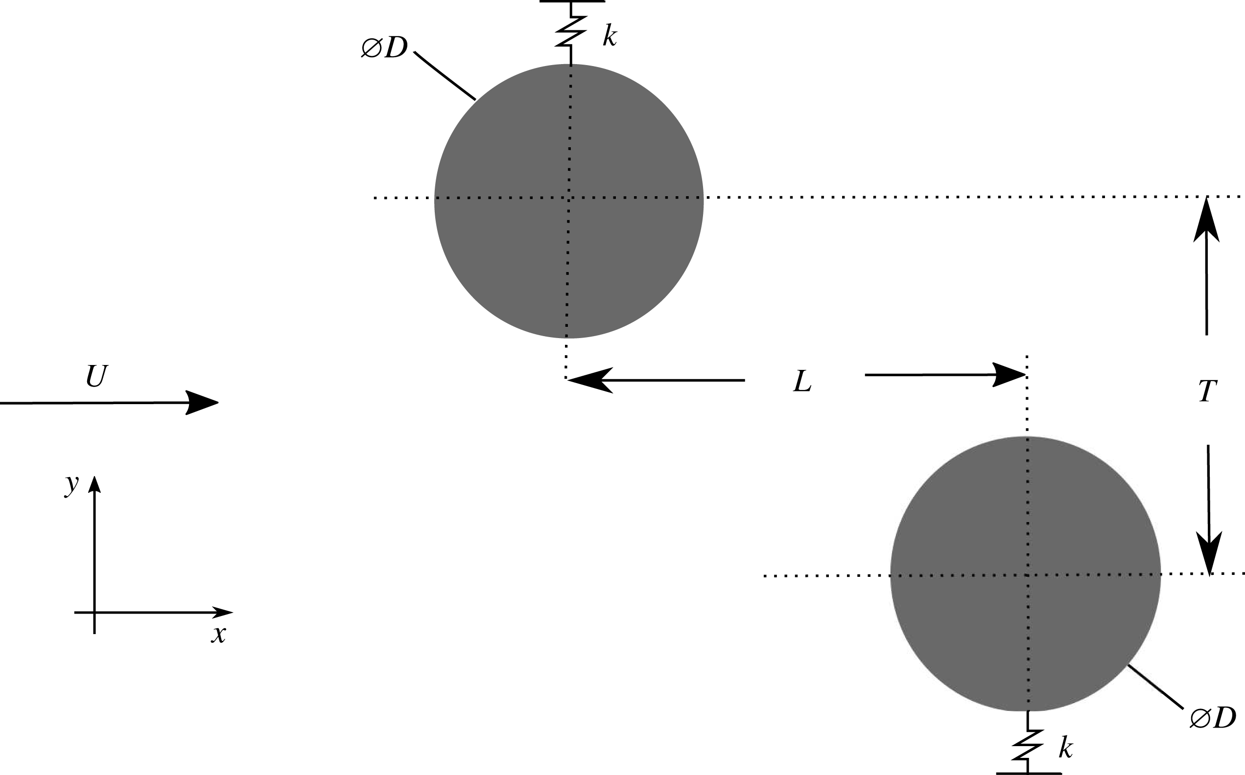
Figure 1 depicts the basic problem set-up of two cylinders in close proximity used for the current study. The streamwise distance between the cylinders of diameter
 $D$
is defined as
 $L$
and the cross-stream distance as
 $T$
. For two cylinders, arrangements are typically classed in three categories: tandem, side-by-side and staggered. Tandem cylinders are arranged inline to the flow (
 $L\geqslant D$
,
 $T=0.0$
). Side-by-side cylinders are side-by-side with respect to the oncoming flow (
 $L=0.0$
,
 $T\geqslant D$
). For staggered cylinders, there is both a streamwise and cross-stream offset (
 $L>0.0$
,
 $T>0.0$
,
 $\sqrt{L^{2}+T^{2}}>D$
). Staggered cylinders arrangements are also often defined in terms of a pitch ratio,
 $P/D$
, where
 $P$
is the distance between the cylinders, and an incidence angle,
 $\unicode[STIX]{x1D6FC}$
.
A schematic of the set-up studied.

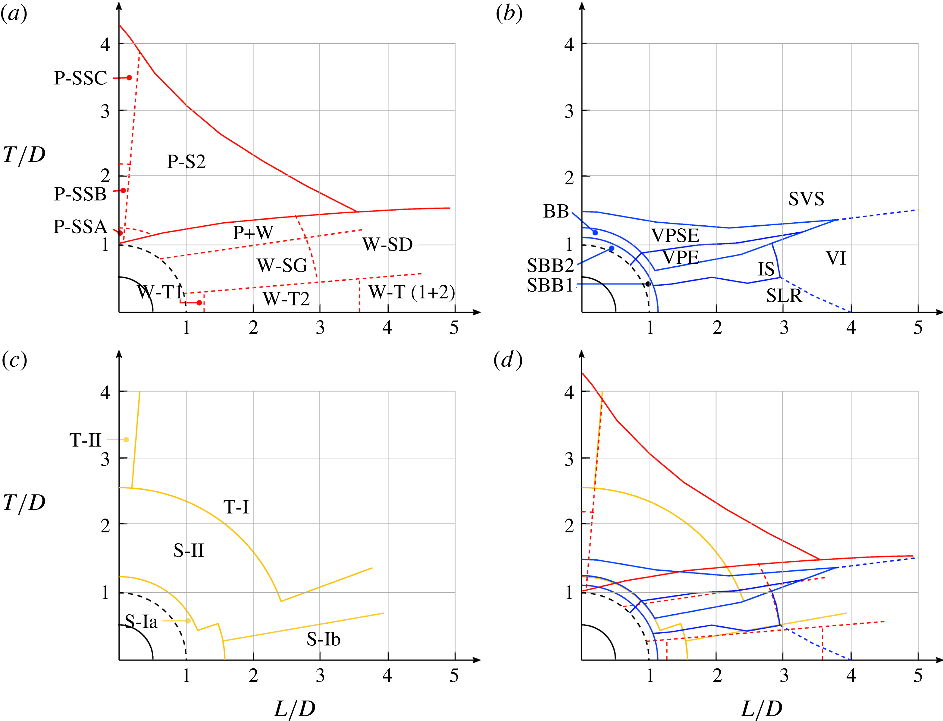
A comparison of the various classification schemes for two fixed cylinders. All distances are centre-to-centre, so that the dashed line at a radius of 1 indicates the centre location of the rearward cylinder where the cylinders’ surfaces touch. Schemes are from (a) Zdravkovich (Reference Zdravkovich1987), (b) Sumner, Price & Paidoussis (Reference Sumner, Price and Paidoussis2000), (c) Hu & Zhou (Reference Hu and Zhou2008) and (d) all three studies combined. Note that the notation used to label the various regimes is taken from the original papers. In spite of the different schemes used, all studies show some correspondence in a series of regimes occurring at a fixed
 $L/D\simeq 2.0$
with increasing cylinder offset
 $T/D$
.

The flow past static cylinders serves as a limiting case and a starting point for examining the vibrating cylinders case. Zhou & Alam (Reference Zhou and Alam2016) provides a recent review of the subject. Here, three previous studies are highlighted that have separately attempted to provide a regime map showing the various flow states that occur as the position of the rearward cylinder is changed relative to the forward cylinder. These regime maps, replotted on common axes at the same scale, are shown in figure 2.
Figure 2(a) shows the map from Zdravkovich (Reference Zdravkovich1987). The Reynolds number is not explicitly stated in that paper. It appears that the data are compiled from a series of studies for subcritical flows (
 $Re<10^{5}$
). The solid lines on the plot are those plotted by Zdravkovich (Reference Zdravkovich1987), the dashed lines indicate approximate boundaries that in the original paper were only described in the text or by approximate hashed regions on the plot. The regimes comprise two main categories: ‘P’ regimes where the flows around each cylinder are modified due to the proximity of the other; ‘W’ regimes where the rearward cylinder is immersed in the wake of the forward cylinder. These main categories are then further decomposed depending on the cylinders’ relative position: tandem (T), staggered (S) and side-by-side (SS). These categories are then decomposed again by a defining flow feature and given either an extra number or letter designation – the reader is referred to the original paper (Zdravkovich Reference Zdravkovich1987) for fuller descriptions of each of the modes delineated in figure 2(a). Distinctions between modes were made based on a combination of scalar measurements such as lift force and frequency, and flow visualisation. It is clear that a rich collection of regimes occurs, with subsequent changes in the shear layers, vortices and other flow features, and temporal behaviour as the flow transits between them. One particular feature to note is the high number of regimes that occur as a function of lateral spacing
 $T/D$
for a longitudinal spacing
 $1.5<T/D<2.5$
.
Figure 2(b) shows the map from Sumner et al. (Reference Sumner, Price and Paidoussis2000). This map was produced using experiments where
 $850<Re<1900$
, and using flow visualisation as the primary identification method. The authors produced an independent, alternative classification scheme to Zdravkovich (Reference Zdravkovich1987) and reclassified the flows into nine regimes: flow where the two bodies acted as a single bluff body with no flow between them (SBB1 and SBB2); flows where the jet formed between the bodies acted as base bleed (BB); flows where the forward cylinder shear layers reattached to the rearward cylinder (SLR); flows where the flow through the gap between the cylinders induced separation of the shear layer from the rearward cylinder (IS); flows where the vortices formed and shed from the front cylinder pair with and envelope the vortices from the rear cylinder (VPE); flows where the front cylinder vortices pair with, envelope and split the vortices from the rear cylinder (VPSE); flows where a clear vortex street is formed from both cylinders individually (SVS); and finally flows where the formed vortices from the forward cylinder impinge on the rearward cylinder (VI). Similar to the scheme from Zdravkovich (Reference Zdravkovich1987), the features chosen to delineate each mode were those that were most distinguishable in the given region of the parameter space. Also of note is the range of modes identified for a longitudinal spacing centred around
 $L/D=2$
.
Figure 2(c) shows the map produced by Hu & Zhou (Reference Hu and Zhou2008). This map was produced using experiments at
 $Re=7000$
, and using particle image velocimetry (PIV) as the primary identification method, guided by flow visualisation of experiments at
 $Re=300$
. Instead of investigating the flow around the two cylinders or the near wake, Hu & Zhou (Reference Hu and Zhou2008) classify flows based on the ‘intermediate’ wake, looking at vortex configurations at a downstream distance
 $x/D=6$
. These regimes comprise two main categories: flows where there is a single wake from both bodies (S) and flows where there are two identifiable, but interacting, wakes, one from each cylinder (T). Each of these categories is further delineated into subcategories: S-I, a single wake with approximately ‘antisymmetric’ vortex shedding (S-Ia has strong vortices with the bodies behaving as one, S-Ib has weaker vortices as the shear layers from the forward body reattach to the rearward body and vortices are effectively shed from the rear body only); S-II, where a vortex street is initially shed from both bodies, but of unequal strength and width, the weaker and narrower shed from the forward cylinder being amalgamated into the wake from the rearward cylinder; T-I, where each body sheds a vortex street, generally at different frequencies, and these streets strongly interact; and T-II, where the two vortex streets occur at the same frequency and form a symmetric pattern.
Figure 2(d) plots all of these maps on the same axes. While there is not a perfect correspondence between the regime boundaries, there is a striking resemblance between them, particularly considering the range of
 $Re$
of the contributing experiments. In particular, when the rearward body is placed in the near wake of the forward body (
 $L/D\simeq 2$
), there is a very close correspondence between all three studies. Note the following, in particular:
-
(i) For
 $T/D\leqslant 0.4$
. Zdravkovich (Reference Zdravkovich1987) labels this regime W-T2: wake interference in an essentially tandem configuration, with the separated shear layers from the forward cylinder reattaching to the rearward cylinder and therefore producing no ‘gap flow’ between the cylinders, and vortices being shed only from the rear cylinder. This description is almost identical to that from Hu & Zhou (Reference Hu and Zhou2008) for their corresponding S-Ib regime. Similarly, the shear layer reattachment (SLR) regime from Sumner et al. (Reference Sumner, Price and Paidoussis2000) is characterised by this same feature.
-
(ii) For
$0.4\leqslant T/D\leqslant 1.0$
. Zdravkovich (Reference Zdravkovich1987) labels this regime W-SG: wake interference in a staggered configuration, with a strong ‘gap flow’, i.e. a significant flow passes through the gap between the cylinders. Sumner et al. (Reference Sumner, Price and Paidoussis2000) identify two regimes in this range with increasing
$T/D$
: first regime IS, where the gap flow is strong enough to induce separation of the boundary layer from the rearward cylinder on the gap side, and then regime VPE, where vortices are shed from the rearward cylinder on the gap side which are paired and enveloped by the vortices from the forward cylinder. Hu & Zhou (Reference Hu and Zhou2008) identify a regime S-II, characterised by unequal-strength vortex streets from both bodies that eventually amalgamate into one wake – a description very reminiscent of the VPE regime from Sumner et al. (Reference Sumner, Price and Paidoussis2000).Taken together these descriptions highlight the importance of the flow between the cylinders in this regime. The fact that there is flow through the gap delineates this regime from the regime at lower
$T/D$
. The effect of the increasing strength of this flow – first inducing separation from the rearward cylinder, and then instigating vortex shedding – is the feature used by Sumner et al. (Reference Sumner, Price and Paidoussis2000) to differentiate the IS and VPE regimes. -
(iii) For
$1.0\leqslant T/D\leqslant 1.3$
. Zdravkovich (Reference Zdravkovich1987) labels this regime P
$+$
W: a combination of proximity interference caused by the interaction of two clearly formed wakes, one from each body, and wake interference, where the rearward body is immersed in the wake of the forward body. Sumner et al. (Reference Sumner, Price and Paidoussis2000) label this region VPSE, with complex vortex pairing, splitting and enveloping occurring between the vortices shed from the forward and rearward bodies on the gap side. Hu & Zhou (Reference Hu and Zhou2008) keep the same designation as the lower
$T/D$
range, i.e. S-II, focusing on the fact that the overall wake eventually amalgamates further downstream. While not explicit in their descriptions, all of these studies hint that this region is temporally complex, with complicated vortex dynamics generated by the fact that the rearward body is almost completely, or completely, exposed to the oncoming flow. This allows almost unfettered shear layer detachment and vortex formation on the outer sides, but ensures a strong interaction between the forming shear layers of opposite-sign vorticity from the two bodies in the gap. -
(iv) For
$T/D>1.3$
. Zdravkovich (Reference Zdravkovich1987) labels this regime P-S2: proximity interference caused by the interaction of two clearly formed wakes, one from each body, in a staggered arrangement with the reference body upstream. Sumner et al. (Reference Sumner, Price and Paidoussis2000) describe this region in a similar fashion, indicating that there are separate vortex streets from each body and labelling the regime SVS. The description from Hu & Zhou (Reference Hu and Zhou2008) initially seems not to match, with two regimes S-II and T-I described with increasing
$T/D$
. However, it should be recalled that Hu & Zhou (Reference Hu and Zhou2008) make their designation based on the vortex configuration at a downstream distance
$x/D\geqslant 6$
. The S-II regime (unequal-strength vortex streets that amalgamate) and the T-I regime (a clear vortex street from each body at different frequency) can both describe the initial formation of two vortex streets that then strongly interact, which is in line with the description of the other studies.




So, it appears that, for moderate downstream separation distances
 $L/D\simeq 2$
, there are three major ‘modes’:
-
(i)
$0\leqslant T/D\leqslant 0.4$
, where there is no net flow through the gap between the cylinders, and vortices are shed only from the rearward cylinder. -
(ii)
$0.4\leqslant T/D\leqslant 1.3$
, where there is a gap flow of increasing strength with increasing
$T/D$
, and the shear layers from the ‘inner’ sides of both bodies interact more strongly with each other than with the corresponding ‘outer’ shear layer from the same body. The formation of a gap jet, or paired and/or amalgamated vortices from the roll-up of the inner shear layers into ‘gap pairs’, is an intrinsic aspect of the dynamics. -
(iii)
$T/D>1.3$
, where the gap becomes large enough for the inner shear layers to interact with the corresponding outer shear layer from the same body, and the vortices roll up into ‘wake pairs’, in a similar fashion to a single isolated cylinder. These wakes can then interact due to their proximity.


These regimes will be used for a base of comparison with the flow-induced vibration cases investigated in this study.
The flow-induced vibration of the cylinders in tandem and side-by-side arrangement has been considered by a number of authors. The tandem elastically mounted cylinder arrangement investigated by Borazjani & Sotiropoulos (Reference Borazjani and Sotiropoulos2009) consisted of an inline offset of
 $L/D=1.5$
, with no cross-stream offset,
 $T/D=0.0$
. The cylinders were found to oscillate at greater amplitudes than a single isolated cylinder and also to experience greater lift force. Borazjani & Sotiropoulos (Reference Borazjani and Sotiropoulos2009) categorised the flows into two states, with state 1 being the state where the front cylinder oscillated at a greater amplitude than the rear, and state 2 where the rear oscillated more. They found that the transition with reduced velocity (
 $U^{\ast }=U/f_{N}D$
, where
 $U$
is the free-stream velocity,
 $f_{N}=\sqrt{k/m}/(2\unicode[STIX]{x03C0})$
is the natural structural frequency,
 $k$
is the spring stiffness coefficient and
 $m$
is the sprung mass) from state 1 to state 2 occurred near
 $U^{\ast }=5$
, identifying the maximum distance reached between the two cylinders,
 $\unicode[STIX]{x1D6FF}y/D$
, as a defining characteristic, with state 1 exhibiting
 $\unicode[STIX]{x1D6FF}y/D<1.0$
and state 2,
 $\unicode[STIX]{x1D6FF}y/D>1.0$
. They also examined the effect of having two degrees of freedom for the cylinder motion.
Other studies have examined similar problem configurations: with two rigidly coupled cylinders in tandem and side-by-side arrangement (Zhao Reference Zhao2013); with side-by-side cylinders with two degrees of freedom (Huera-Huarte & Gharib Reference Huera-Huarte and Gharib2011); with tandem cylinders with the upstream cylinder stationary and the downstream oscillating (Assi et al.
Reference Assi, Bearman and Meneghini2010; Carmo, Assi & Meneghini Reference Carmo, Assi and Meneghini2013), tandem and staggered cylinders with two degrees of freedom (Assi Reference Assi2014), and tandem cylinders of unequal size (Wang et al.
Reference Wang, Yang, Nguyen and Yu2014); with two tandem cylinders vibrating with two degrees of freedom (Huera-Huarte & Gharib Reference Huera-Huarte and Gharib2011); and with two and three tandem cylinders (
 $L/D=4.0$
) oscillating with two degrees of freedom (Yu et al.
Reference Yu, Étienne, Scolan, Hay, Fontaine and Pelletier2016). There has been no comprehensive study of the flow-induced vibrations of two staggered cylinders.
The current study proposes to build on work in the literature, investigating flows past cylinders with tandem arrangements, and then extending to staggered arrangements by varying the cross-stream offset
 $T$
, for both static and elastic cylinder mountings. Given the large range of parameters to consider in addressing the flow-induced vibration of staggered cylinders (
 $L/D$
,
 $T/D$
, reduced velocity
 $U^{\ast }$
, damping
 $c^{\ast }=cD/(mU)$
, mass ratio
 $m^{\ast }=4m/(\unicode[STIX]{x1D70C}D^{2}l)$
, and the Reynolds number
 $Re=UD/\unicode[STIX]{x1D708}$
, where
 $c$
is the damping coefficient,
 $\unicode[STIX]{x1D70C}$
is the fluid density,
 $l$
is the length of the cylinder and
 $\unicode[STIX]{x1D708}$
is the kinematic viscosity), the current study has restricted its focus. The case investigated in Borazjani & Sotiropoulos (Reference Borazjani and Sotiropoulos2009) (
 $L/D=1.5$
,
 $T/D=0.0$
,
 $c^{\ast }=0$
,
 $m^{\ast }=2.546$
,
 $3\leqslant U^{\ast }\leqslant 14$
,
 $Re=200$
, with the motion constrained to the cross-flow direction) is used as a base case and starting point for the current investigation. Note that in some sense this is a limiting case, where the damping
 $c^{\ast }=0$
, which would be effectively impossible to achieve experimentally. However, such a limiting case is informative of the range of behaviour possible, as the dynamic response of the structure should be maximised. The value of
 $L/D$
selected also puts the cylinders at a distance that traverses the three modes of response identified for static cylinders outlined above as
 $T/D$
is varied.
The paper proceeds as follows. Section 2 defines the problem studied and the specification of the bodies and mounting. Section 3 describes the numerical method and set-up. Section 5 presents the results, with the regimes across the entire parameter space shown in § 5.1, followed by more discussion of the limiting cases at
 $U^{\ast }=0$
and
 $T/D=0.0$
in §§ 5.2 and 5.3, respectively. Section 5.4 describes flows for vibrating cylinders and staggered configurations. The validity of the work and the applicability of the results are discussed in § 6. Concluding remarks follow in § 7.
2 Problem definition
Figure 1 outlines the problem set-up. In the results presented here, the upstream cylinder is positioned at
 $x=-L/(2D)$
,
 $y=T/(2D)$
and the downstream cylinder is at
 $x=L/(2D)$
,
 $y=-T/(2D)$
.
The ratio of the mass of each cylinder to the mass of the equivalent volume of fluid is defined as
 $m^{\ast }=2.546$
, as used in Borazjani & Sotiropoulos (Reference Borazjani and Sotiropoulos2009) in their study of tandem vibrating cylinders. Each cylinder is elastically mounted with identical natural frequencies, and therefore reduced velocity,
 $U^{\ast }$
. There is no damping added to the system,
 $c^{\ast }=0$
. The
 $y$
-position of a cylinder is defined as
 $Y$
and the oscillation of each cylinder is defined by the equation:
 $$\begin{eqnarray}\left.\begin{array}{@{}c@{}}m[\ddot{Y_{1}}+(2\unicode[STIX]{x03C0}f_{N})^{2}(Y_{1}-(T/2))]=F_{y_{1}},\\ m[\ddot{Y_{2}}+(2\unicode[STIX]{x03C0}f_{N})^{2}(Y_{2}+(T/2))]=F_{y_{2}},\end{array}\right\}\end{eqnarray}$$
where
 $\ddot{Y}$
is the acceleration of the cylinder perpendicular to the free stream and
 $F_{y}$
is the lift force on the cylinder. In non-dimensional form, these equations can be expressed as
 $$\begin{eqnarray}\left.\begin{array}{@{}c@{}}\displaystyle \unicode[STIX]{x03C0}m^{\ast }\left[\frac{\ddot{y_{1}}}{2}+\frac{\unicode[STIX]{x03C0}^{2}m^{\ast }}{U^{\ast 2}}\left(y_{1}-\frac{T/D}{2}\right)\right]=C_{L_{1}},\\ \displaystyle \unicode[STIX]{x03C0}m^{\ast }\left[\frac{\ddot{y_{2}}}{2}+\frac{\unicode[STIX]{x03C0}^{2}m^{\ast }}{U^{\ast 2}}\left(y_{2}-\frac{T/D}{2}\right)\right]=C_{L_{2}},\end{array}\right\}\end{eqnarray}$$
where
 $y$
is the non-dimensional cylinder displacement
 $Y/D$
, and
 $C_{L}$
is the transverse (lift) force coefficient per unit length,
 $C_{L}=2F_{y}/(\unicode[STIX]{x1D70C}U^{2}D)$
. Hence, the position of the cylinders can be described as
 $$\begin{eqnarray}\left.\begin{array}{@{}c@{}}\displaystyle y_{1}=\overline{y}_{1}+{y^{\prime }}_{1}+(T/D)/2,\\ \displaystyle y_{2}=\overline{y}_{2}+{y^{\prime }}_{2}-(T/D)/2,\end{array}\right\}\end{eqnarray}$$
where
 $\overline{y}_{n}$
is the non-dimensional mean position of cylinder
 $n$
with respect to the cylinder starting point and
 ${y^{\prime }}_{n}$
is the oscillatory component of the non-dimensional motion of cylinder
 $n$
. The subscripts 1 and 2 denote the front and rear cylinders, respectively. The cylinders are in a uniform free-stream flow and the Reynolds number is 200.
3 Method
Simulations were carried out using a sharp-interface immersed-boundary method, in which the vibrating cylinders are represented by a Lagrangian set of finite elements immersed in an underlying Cartesian grid. The basic method follows closely that outlined in Mittal et al. (Reference Mittal, Dong, Bozkurttas, Najjar, Vargas and von Loebbecke2008), and further details of the implementation used here for fluid–structure interaction problems is provided in (Griffith & Leontini Reference Griffith and Leontini2017). A concise description of the method is provided below.
The flow is simulated by solving the incompressible Navier–Stokes equations
 $$\begin{eqnarray}\left.\begin{array}{@{}c@{}}\displaystyle \frac{\unicode[STIX]{x2202}\boldsymbol{u}}{\unicode[STIX]{x2202}\unicode[STIX]{x1D70F}}=-(\boldsymbol{u}\boldsymbol{\cdot }\unicode[STIX]{x1D735})\boldsymbol{u}-\unicode[STIX]{x1D735}P+\frac{1}{Re}\unicode[STIX]{x1D6FB}^{2}\boldsymbol{u},\\ \displaystyle \unicode[STIX]{x1D735}\boldsymbol{\cdot }\boldsymbol{u}=0,\end{array}\right\}\end{eqnarray}$$
where
 $\unicode[STIX]{x1D70F}=tU/D$
is the time non-dimensionalised by the advective time scale,
 $\boldsymbol{u}$
is the velocity field non-dimensionalised by the free-stream velocity
 $U$
, and
 $P$
is the pressure field non-dimensionalised by
 $\unicode[STIX]{x1D70C}U^{2}$
. These equations were solved by discretising in space using a second-order central finite-difference scheme. To integrate the equations forward in time, a two-way time-splitting scheme in employed.
First, the advection and diffusion terms (the first and third terms in the momentum equation (3.1), respectively) are integrated to an intermediate time between the start and end of the time step, over a first ‘substep’. The numerical scheme employed for the advection term was an explicit second-order Adams–Bashforth scheme, whereas an implicit second-order Crank–Nicolson scheme was employed for the diffusion term. The resulting implicit equation was solved using Gauss–Jacobi iteration.
Second, the pressure term was integrated from this intermediate time to the end of the step, over a second substep. For this to occur, the pressure correction (the amount the pressure field had changed with respect to the previous time step) needed to be first evaluated. This was done by taking the divergence of the pressure substep equation, and enforcing continuity (i.e. that the velocity field is divergence-free), resulting in a Poisson equation for the pressure correction. This Poisson equation was solved using a hand-coded geometric multigrid method.
The velocity and pressure fields were collocated on the same cell-centred mesh. To avoid ‘chequerboarding’, or odd–even decoupling of the pressure field, a process of interpolating from cell-centred values to face-centred values was employed between the two substeps, and the resulting values were used to form the right-hand side of the pressure Poisson equation.
The immersed boundaries of the two cylinders were imposed using an interpolation scheme for values at mesh points that were immediately inside the body (those points that were inside the body, but had an immediate neighbour point outside the body), essentially forming a modified stencil for these points. This interpolation scheme maintained the overall order of accuracy of the differencing scheme. While such an interpolation scheme can lead to spurious oscillations in the pressure field that the distributed-force immersed-boundary scheme does not suffer from, the interpolation has the advantage of maintaining a sharp representation of the boundary, which can be important for multiple bodies in proximity. It should be noted that a recent study has shown that these spurious oscillations pose no problem for fluid–structure problems as long as the resolution of the mesh is adequate (Griffith & Leontini Reference Griffith and Leontini2017).
The vibration of each cylinder is found by solving (2.1) in conjunction with the Navier–Stokes equations (3.1) using a Newmark-
 $\unicode[STIX]{x1D6FD}$
method, employing the standard value of
 $\unicode[STIX]{x1D6FD}=0.25$
(Newmark Reference Newmark1959). A free-stream Dirichlet boundary condition was imposed for the velocity on the upstream and transverse boundaries,
 $\boldsymbol{u}=U$
, and a Neumann condition for the velocity was imposed at the downstream boundary,
 $\unicode[STIX]{x2202}\boldsymbol{u}/\unicode[STIX]{x2202}n=0$
. For the pressure, a Neumann condition was imposed on the upstream and transverse boundaries,
 $\unicode[STIX]{x2202}P/\unicode[STIX]{x2202}n=0$
, and a Dirichlet condition imposed at the downstream outlet,
 $P=0$
. On the immersed-boundary surface, the velocity of the fluid was set to match the velocity of the body, while the normal pressure gradient was set to zero.
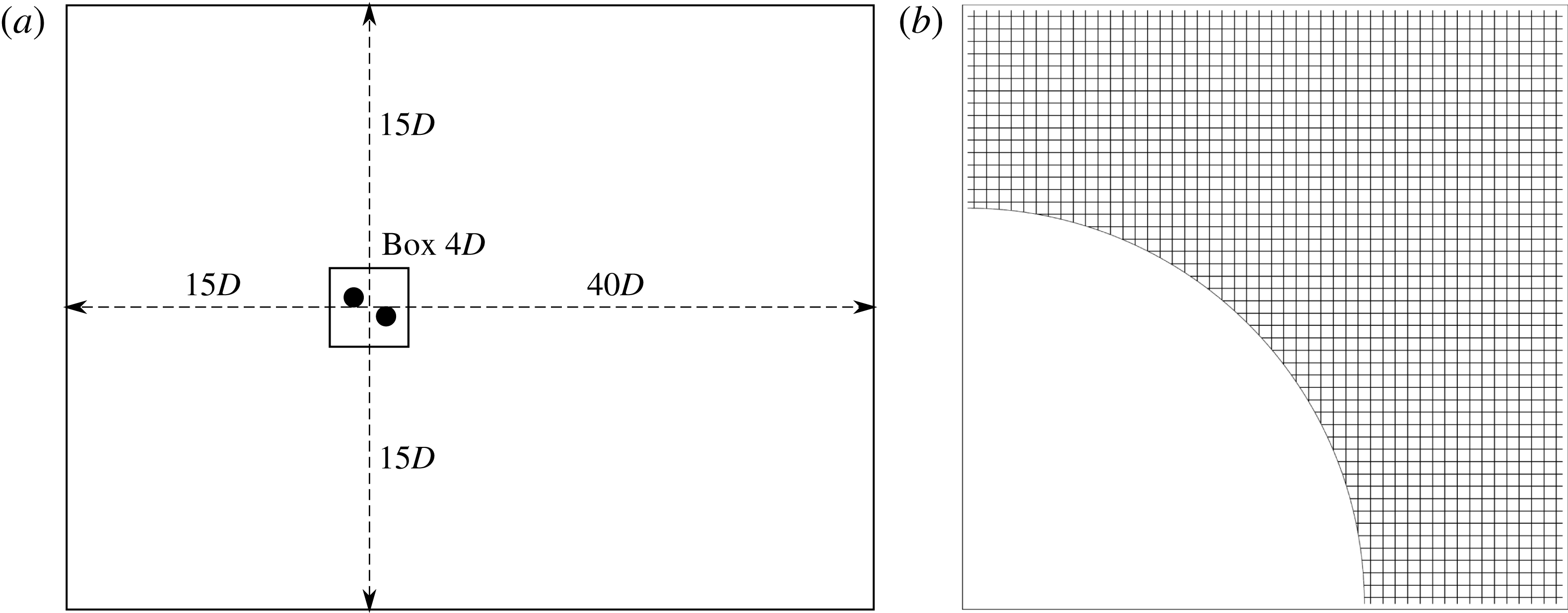
The underlying Cartesian grid was designed with a regular grid spacing around the origin, over a box region measuring
 $4D$
in each direction. Grid spacings were then increased linearly to the domain boundaries. The inlet and lateral domain boundaries were located
 $15D$
from the origin, while the outlet boundary was located
 $40D$
downstream. Twice as many grid points were used in the streamwise direction as in the transverse direction; the number of grid points in each direction is restricted to powers of 2, thereby leading to a grid size of
 $2^{N+1}\times 2^{N}$
, where
 $N$
is a whole number. We denote each grid as
 $MN$
, such that
 $M10$
corresponds to a grid size of
 $2048\times 1024$
nodes.
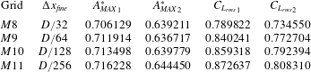
Maximum oscillation amplitudes and r.m.s. lift coefficients for the four immersed-boundary grids tested, for the tandem cylinder arrangement of offset
 $T=0.0$
and with reduced velocity
 $U^{\ast }=5$
. The subscripts 1 and 2 refer to the front and rear cylinders, respectively.
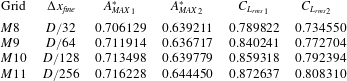
A test of the sensitivity of the results to grid resolution was carried out. For the tandem cylinder arrangement of offset
 $T=0.0$
, results were obtained over the
 $U^{\ast }$
range for grids
 $M8$
,
 $M9$
,
 $M10$
and
 $M11$
. Table 1 presents the results for
 $U^{\ast }=5$
returned for maximum cylinder displacement,
 $A_{MAX}^{\ast }$
, and root-mean-square (r.m.s.) lift coefficient,
 $C_{L_{rms}}$
, for the two cylinders, the front and rear cylinders being denoted by subscripts 1 and 2. For the grid
 $M9$
, the results returned for
 $A_{MAX}^{\ast }$
are within 1 % of the result returned by the higher-resolution
 $M10$
grid, while the r.m.s. value of the lift coefficient is within 2 %. For all the results presented here for
 $T/D\leqslant 3.5$
, grid
 $M9$
was used. For the upper range of cylinder offset,
 $T/D>3.5$
, the box region of regular grid spacing around the origin was increased to
 $8D$
in the
 $y$
-direction to encompass the wider wake width and cylinder vibration that these cylinder arrangements produce. For this grid the number of total grid points in the
 $y$
-direction was doubled for the
 $M9$
grid, maintaining the same transverse domain boundary distance, but using the extra grid points to increase the size of the box region of regular grid spacing. Simulations run for values of
 $T/D<3.5$
using both grids showed negligible differences in oscillation amplitude and mean force coefficient. A schematic of the mesh set-up, along with an image showing the resolution of the utilised
 $M9$
mesh in the vicinity of the cylinders, is shown in figure 3.
(a) A schematic of the regions defined that control the mesh resolution. (b) A close-up of the mesh in the vicinity of the cylinders.

All simulations were run for a minimum of
 $\unicode[STIX]{x1D70F}=1000$
, to ensure reliable statistics and frequency content could be measured.
4 Validation
Here, a brief validation study of the vortex-induced vibration of a single elastically mounted cylinder is presented. A more in-depth treatment of the validation of the code, control of error and details of the implementation can be found in Griffith & Leontini (Reference Griffith and Leontini2017). For this validation study, the mass ratio is set to
 $m^{\ast }=1$
, which is lower than the mass ratio used for the two-cylinder problem (
 $m^{\ast }=2.546$
) that is the focus of the current study. Lower body mass typically leads to larger accelerations, and therefore provide a more difficult test of a numerical scheme.
The response of a single elastically mounted cylinder for
 $Re=200$
and
 $m^{\ast }=1$
. (a) The maximum amplitude of oscillation obtained at any time,
 $A_{MAX}^{\ast }$
. (b) The maximum lift coefficient obtained at any time,
 $C_{L_{MAX}}$
. (c) The primary frequency of oscillation. Results obtained using a spectral-element method (Thompson et al.
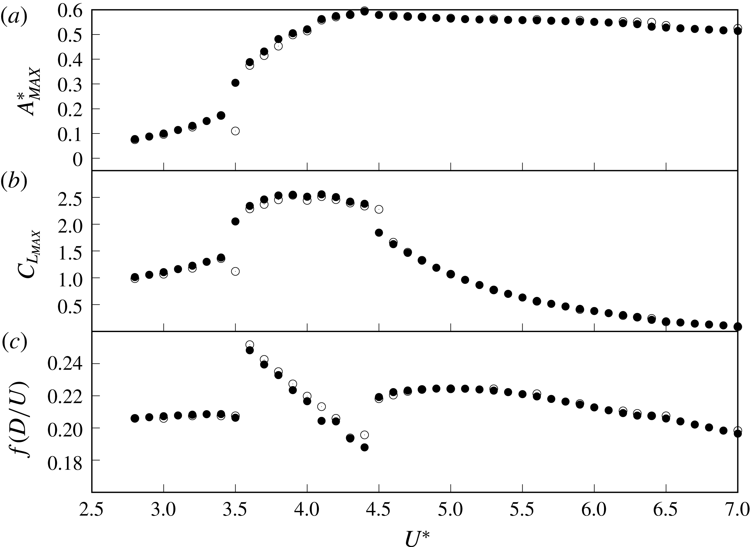
Reference Thompson, Hourigan and Sheridan1996) (●) and the current immersed-boundary scheme using the M9 mesh (○). The results from both codes are very similar across the entire parameter space.

Figure 4 presents the response of the single cylinder in terms of the maximum amplitude of oscillation
 $A_{MAX}^{\ast }$
, the maximum lift coefficient
 $C_{L_{MAX}}$
and the primary frequency of oscillation as functions of the reduced velocity
 $U^{\ast }$
. The results of the immersed-boundary code are plotted along with results from a well-validated spectral-element code (see Thompson et al. (Reference Thompson, Hourigan and Sheridan1996) and Leontini et al. (Reference Leontini, Thompson and Hourigan2006) for an explanation of the method and a relevant validation case).
It is clear that the two codes, based on two completely different schemes, produce very similar results. This provides confidence in the ability of the immersed-boundary code to accurately capture the dynamics of the fluid–structure system. Further comparison with published data from Borazjani & Sotiropoulos (Reference Borazjani and Sotiropoulos2009) is made in § 5.3, providing more evidence that the dynamics are accurately captured.
It should also be noted that the upper limit of the maximum amplitude for both codes,
 $A_{MAX}^{\ast }\simeq 0.6$
, compares very well to the upper limit for laminar vortex-induced vibration deduced from the data compiled in Williamson & Govardhan (Reference Williamson and Govardhan2004).
5 Results
5.1 Regimes mapped across the parameter space of
$U^{\ast }$
,
$T/D$


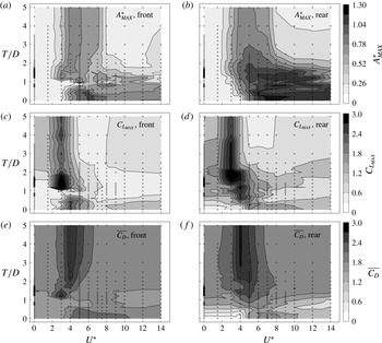
We first present data maps for the entire reduced velocity–cross-stream offset parameter space, before examining particular cases. Figure 5 plots contours of maximum oscillation amplitude,
 $A_{MAX}^{\ast }$
, maximum coefficient of lift,
 $C_{L_{MAX}}$
, and mean coefficient of drag,
 $\overline{C_{D}}$
, over the range of reduced velocity,
 $0.0\leqslant U^{\ast }\leqslant 14.0$
, and cross-stream offset,
 $0.0\leqslant T/D\leqslant 5.0$
. The left-hand panels show data for the upstream cylinder and the right-hand panels data for the downstream cylinder. Value
 $T/D=0.0$
indicates the cylinder arrangement where the upstream and downstream cylinders have their origins at
 $\{x_{0},y_{0}\}=\{-0.75,0.0\}$
and
 $\{0.75,0.0\}$
; that is, the tandem case. The maximum value of cylinder offset,
 $T/D=5.0$
, indicates an arrangement where the cylinders are free to oscillate in the cross-stream direction around
 $\{x_{0},y_{0}\}=\{-0.75,2.5\}$
and
 $\{0.75,-2.5\}$
. For the reduced velocity, low values of
 $U^{\ast }$
mean stiff elastic mountings, with
 $U^{\ast }=0.0$
implying entirely static non-vibrating cylinders. As reduced velocity,
 $U^{\ast }$
, increases, the elastic mounting becomes slacker.
Over the
 $U^{\ast },T/D$
parameter space, (a,b) contours of maximum amplitude of oscillation,
 $A_{MAX}^{\ast }$
, (c,d) contours of maximum coefficient of lift,
 $C_{L_{MAX}}$
, and (e,f) contours of mean coefficient of drag,
 $\overline{C_{D}}$
. Maxima are calculated as an average of the greatest 10 % of peaks. Panels on the left are for the upstream cylinder and on the right for the downstream.

The two contour maps for maximum oscillation amplitude,
 $A_{MAX}^{\ast }$
, show those arrangements that result in the largest displacements for the front and rear cylinders. For the front cylinder, the largest excitation occurs at low and zero cross-stream offset,
 $T/D$
, and in the range
 $5.0\leqslant U^{\ast }\leqslant 8.0$
. When the offset is increased further, the maximum amplitude decreases before converging towards the result for a single isolated cylinder, which is evident from the increasingly vertical contour lines, with
 $T/D$
. For the higher reduced velocities, the maximum amplitude oscillation occurs around
 $T/D=0.0$
and is greater than the result of the single isolated cylinder.
As evident from the darker contours, the rear cylinder oscillates at a greater amplitude than the front cylinder for large parts of the parameter space. The greatest amplitude occurs for low values of
 $T/D$
and in the reduced velocity range
 $6.0\leqslant U^{\ast }\leqslant 11.0$
.
The contours of maximum coefficient of lift,
 $C_{L_{MAX}}$
, show the highest values for
 $U^{\ast }=3.0$
and
 $4.0$
, and intermediate transverse
 $T/D\simeq 1$
. It is proposed that this is due to the strong influence of the flow and subsequent vortex formation through the gap between the cylinders, similar to the mechanism of excitation for wake-induced vibration proposed by Assi et al. (Reference Assi, Bearman and Meneghini2010); this point is further expanded on in § 5.4.
For the mean coefficient of drag,
 $\overline{C_{D}}$
, the two cylinders give similar contour maps, except for those cases where the downstream cylinder lies mostly, or entirely, in the wake of the upstream cylinders, thereby hiding it from the oncoming free-stream flow. The cases producing the lowest mean drag on the rear cylinder are the tandem cases at low and zero reduced velocity; for these cases, the amplitude of oscillation is very small, meaning the rear cylinder never, or hardly, comes out from behind the upstream cylinder. Drag increases on the downstream cylinder as the offset,
 $T/D$
, increases, resulting in the downstream cylinder meeting more of the free-stream flow, and as the reduced velocity increases. As the reduced velocity increases, the amplitude of oscillation increases, with the increased drag on the downstream cylinder indicative of a phase difference between the two cylinder oscillations, which is discussed more later in the study (see § 5.3).
There are two broad regimes in the parameter space which can be differentiated by the orientation of the contours in figure 5. For higher values of reduced velocity,
 $U^{\ast }>8.0$
, that is, less spring stiffness, the contours are mostly aligned horizontally. This indicates a stronger dependence of behaviour on cylinder cross-stream offset,
 $T/D$
, than on reduced velocity,
 $U^{\ast }$
, or spring stiffness. For reduced velocity,
 $U^{\ast }<8.0$
, stiffer springs, the dependence is less on offset,
 $T/D$
, and more on
 $U^{\ast }$
. The exception to both these categorisations is the section of parameter space around
 $T/D=1.0$
. Here, there is strong variation with offset, around for example
 $U^{\ast }=5.0$
, and some variation with reduced velocity, around for example
 $U^{\ast }\approx 10.0$
.
Across the parameter space, there are a number of frequencies present in the dynamics of the system, the effects of which vary throughout. Firstly, for an isolated, single cylinder at Reynolds number
 $Re=200$
, the vortex shedding frequency, or Strouhal frequency, is
 $St=0.198$
. For rigid cylinders, with increasing cross-stream offset, the frequency of the lift force on both cylinders is expected to approach this value. When the cylinders are close to each other, the vortex formations will be affected, so the frequency will likely change. As reduced velocity increases, the natural frequency of the elastic mounting,
 $f_{N}(D/U)=1/U^{\ast }$
, initially becomes more important. As reduced velocity increases further, the forcing of the spring becomes weaker and the cylinders are more free to move in response to the fluid forcing. For
 $U^{\ast }=\infty$
, the cylinders are entirely free to move and effectively have no equilibrium position.
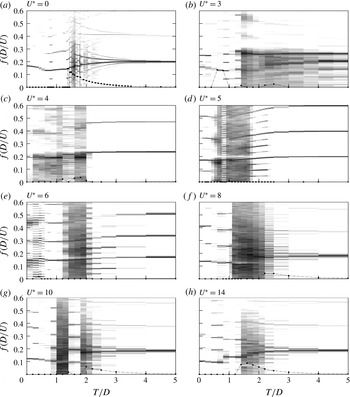
The frequency content of the lift signal on the rear cylinder across the offset,
 $T$
, range and for eight values of reduced velocity,
 $U^{\ast }$
. Each plot is formed by calculating the frequency spectrum for each case of
 $T/D$
, normalising each spectrum by its maximum, and then ‘stacking’ the spectra next to each other. Dark regions represent intensity of a given frequency in the lift signal for a given
 $T/D$
. Contour values vary from white,
 $1\times 10^{-6}$
, to black,
 $1$
. Also shown with dots is the difference in primary frequencies of the two cylinders.

Figure 6 is a compilation of the frequency content of the lift force on the rear cylinder, across the range of
 $T/D$
tested and for eight values of
 $U^{\ast }$
. To construct the plots, the frequency spectra for each case of
 $T/D$
are normalised by their maximum and then stacked next to each other, thereby showing the variation of frequency intensity in the fluid forcing as the offset is changed. Looking first at the plot for reduced velocity,
 $U^{\ast }=0.0$
, for the tandem case,
 $T/D=0.0$
, there is a single dominant frequency,
 $f(D/U)=0.169$
. This is lower than the value for a single isolated cylinder,
 $0.198$
. The single frequency is due to the fact that there is no flow through the gap between the cylinders, and the two cylinders effectively behave as a single body with vortex shedding from the rear cylinder only. As offset increases, this frequency initially decreases, then increases again, until at offset of approximately 1.4 a broadband response is evident, indicating a quasi-periodic or chaotic fluid forcing and flow; the frequency content here will be investigated further in the following section (§ 5.2). As offset increases towards 5.0, the single dominant frequency emerges again, converging to the frequency for a single cylinder.
Note that the term ‘chaos’ here refers to a response that is not periodic, and has a spectrum that contains at least three incommensurate frequencies. Such a response does not appear to repeat over any time scale, and as such this definition is the same as that used in dynamic systems.
For the cases shown where the cylinders are free to vibrate,
 $U^{\ast }=3.0$
, 4.0, 5.0, 6.0, 8.0, 10.0 and 14.0, a range of responses are evident. The dark areas represent broadband response, indicating quasi-periodic or chaotic flows. The two maps most qualitatively similar are the maps for reduced velocities,
 $U^{\ast }=0.0$
and
 $14.0$
. Out of the cases shown, these two cases are effectively the cases where the frequency and forcing of the elastic mounting are the weakest, i.e. where there is effectively no response at the body’s natural frequency. For
 $U^{\ast }=0.0$
, the cylinders do not vibrate at all, while for
 $U^{\ast }=14.0$
, the springs are slack, meaning that, for both, the fluid forcing dominates, thereby giving similar frequency content maps (note that the data for
 $U^{\ast }=0.0$
have higher resolution in
 $T/D$
than the other reduced velocities tested).
An example case where the elastic mounting does play a significant role is reduced velocity
 $U^{\ast }=5.0$
. For the tandem configuration,
 $T/D=0.0$
, the oscillation is periodic, dominated by the primary frequency, which is slightly below the natural frequency of the structure. The other frequency that appears for zero offset is the third harmonic of the primary. Energy in these odd harmonics is indicative of the spatio-temporal symmetry in the forcing on the cylinder. Once an offset is introduced, this symmetry is broken and the second harmonic increases in strength. Periodic vortex shedding persists until the offset,
 $T/D$
, is equal to
 ${\approx}0.6$
. In the cylinder offset range
 $0.6\leqslant T/D\leqslant 1.8$
, the spectra of the lift coefficient signal is not periodic. The more broadband spectrum indicates irregular, perhaps chaotic, vortex shedding. Beyond
 $T/D\approx 1.7$
, the shedding becomes more regular, with the broadband noise decreasing. In the range
 $1.7\leqslant T/D\leqslant 2.4$
, the second and third harmonics are distinct as well as frequencies spaced at one quarter of the primary frequency, indicative of quasi-periodic or period-doubling behaviour. This pattern abruptly ends for
 $T/D=2.4$
and the vortex shedding becomes dominated by a single frequency.
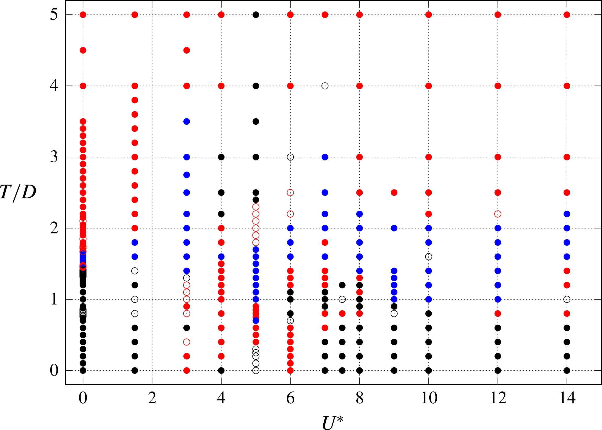
The parameter space, mapped by oscillation frequency content of the coefficient of lift signals of the two cylinders. Symbols are the following: solid black points denote periodic flows, with both cylinders oscillating at the same frequency; hollow black dots denote periodic oscillations, but with period-doubling, or P
 $_{2}$
, oscillations; hollow red dots denote periodic oscillations, with period-multiplying P
 $_{N>2}$
oscillations; solid red dots denote quasi-periodicity; while blue dots represent chaotic oscillations.

Figure 7 provides a summary of the temporal behaviour over the parameter space, where individual cases have been inspected and categorised as being periodic on the period of vortex shedding, periodic over some multiple of the period of vortex shedding, quasi-periodic, or chaotic. Figure 7 gives an overview of the temporal behaviour of the cylinder oscillations over the parameter space; examples of specific cases appear later in the following subsections. Solid black points represent cases where the oscillations are periodic and synchronised. Hollow black points represent cases where the oscillations are still periodic and synchronised, but are period doubling, the flow repeating over two cycles of oscillation. These oscillations are designated as P
 $_{2}$
. The hollow red points present oscillations that are again periodic, but repeat over
 $N$
cycles, where
 $N>2$
. The distinction between P
 $_{2}$
and P
 $_{N>2}$
oscillation has been made to represent the increasing period of the oscillations as
 $N$
increases, which quickly becomes difficult to differentiate from a quasi-periodic response.
The solid red points represent cases where the oscillations of the cylinders are quasi-periodic. This includes quasi-periodicity arising from disordered vortex shedding, but also from small differences in the primary frequency of the oscillation of the two cylinders. For example, the periodic synchronised oscillation for
 $U^{\ast }=5.0$
and
 $T/D>2.5$
is only present for a narrow range of reduced velocity. For the other reduced velocities tested, at
 $T/D=4.0$
and
 $5.0$
, the oscillations are strictly quasi-periodic. However, this is due to each cylinder effectively shedding independently, but with a small difference persisting in the frequency of vortex shedding of the upstream and downstream cylinders. The wakes are interacting in that the presence of one cylinder slightly changes the vortex shedding frequency of the other, but that is the extent of the interaction. In figure 7, we have not attempted to distinguish between weak and strong quasi-periodicity. The frequency content plots of figure 6 give some indication as to the level of complexity of the flow and body oscillations over the parameter space in the quasi-periodic regions.
Also plotted in figure 7 are solid blue points; these represent cases classified as chaotic. The distinction between quasi-periodic and chaotic flows is made chiefly on inspection of Lissajous plots of the cylinder displacements (plots of the displacement of the front cylinder as a function of the displacement of the rear cylinder); where the orbits do not immediately appear simply modulated, we have classified the flow as chaotic. This distinction is subjective; therefore the boundary between solid blue and red points on figure 7 is fuzzy. Nonetheless, it serves as an approximation of regions of the parameter space where the flows are the most disordered.
The parameter space, mapped by oscillation and vortex shedding mode. Shaded grey areas denote regions of the parameter space where cylinder oscillations are periodic and synchronised.

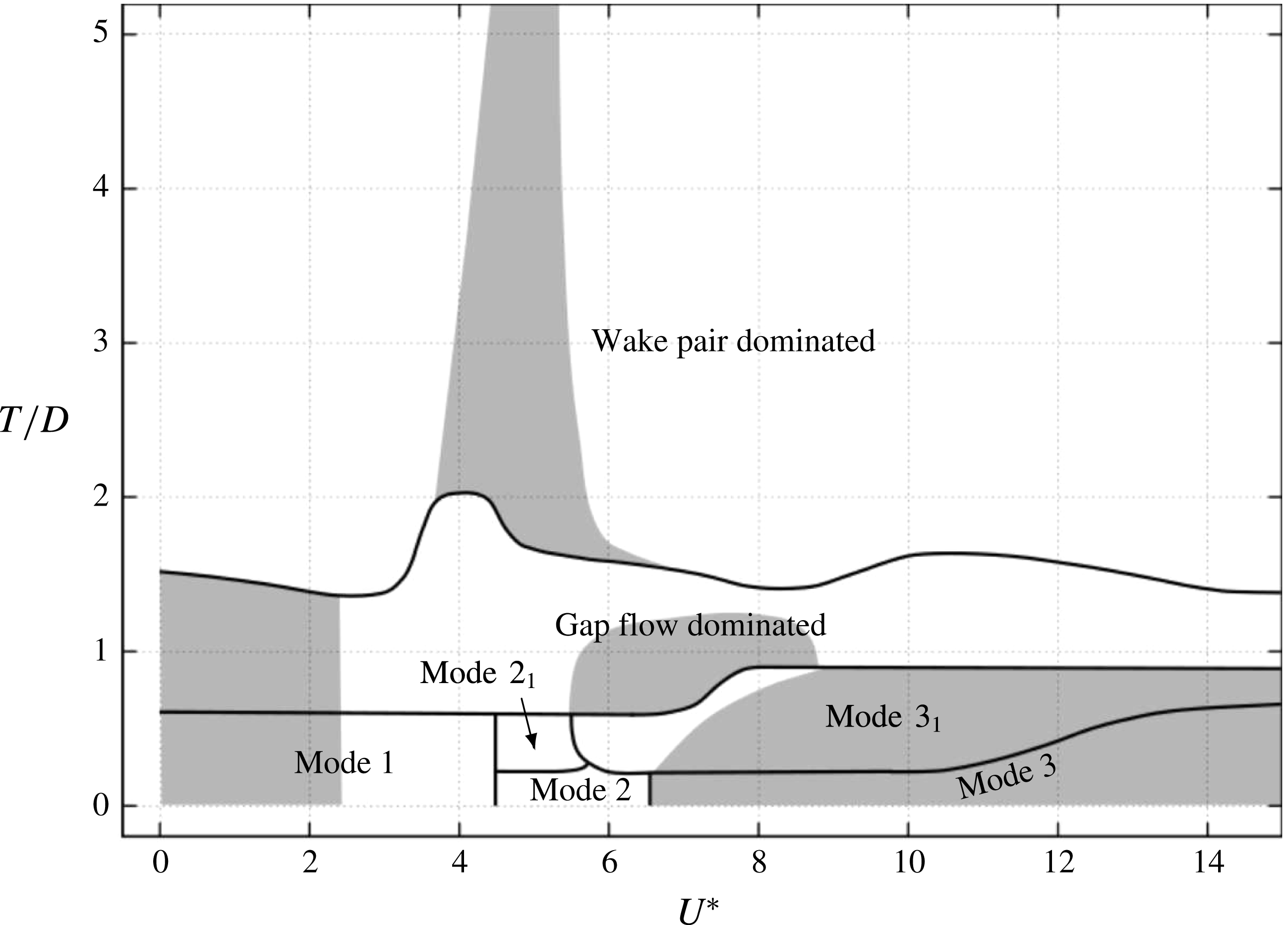
Figure 8 attempts to categorise each case by the type of vortex formation on each cylinder, based on such information as which cylinder sheds or does not shed vortices, whether there is significant flow in the gap between the cylinders and which vortices pair. For the tandem cases we have adopted a similar classification as used by Borazjani & Sotiropoulos (Reference Borazjani and Sotiropoulos2009), describing the low reduced velocity
 $U^{\ast }<5.0$
cases as mode 1. Borazjani & Sotiropoulos (Reference Borazjani and Sotiropoulos2009) denoted
 $U^{\ast }\,\geqslant 7.0$
cases as state 2, and flows in the range
 $5.0\leqslant U^{\ast }\leqslant 6.0$
as a critical state, between states 1 and 2. Instead, we choose to denote their state 2 as mode 3, and the critical state as mode 2. Discussion of these tandem modes will be continued in § 5.3.
The tandem modes only survive a short time for small cross-stream offsets. Modes
 $2_{1}$
and
 $3_{1}$
are one-sided versions of the tandem modes. The region marked as ‘Gap flow dominated’ indicates states where the flow between the cylinders dominates, with the flow characterised by pairing of either shear layers or vortices from the inside side of each cylinder. This region is centred around offset
 $T/D=1.0$
, and is generally characterised by smaller-amplitude and quasi-periodic or chaotic oscillations. At greater cylinder offset, the ‘Wake pair dominated’ region occurs. Instead of gap pairs of vortices and shear layers dominating, the flow is composed of pairs of vortices shed from the same cylinder in a similar manner to the shedding from a single isolated cylinder.
Regions of periodic synchronised oscillation (both cylinders having the same primary frequency) identified in figure 7 are included as greyed regions on figure 8. The cylinders (or lift coefficient in the case of the rigid
 $U^{\ast }=0.0$
cases) oscillate at the same primary frequency when reduced velocity and cross-stream offset are both near zero. Periodicity occurs for high reduced velocity and low offset and tandem cases, and for a narrow band of reduced velocity at offset
 $T/D>2.0$
.
Interestingly, when the cylinders are in close proximity, for
 $T/D<2$
, the oscillation is disordered and not periodic around
 $U^{\ast }=5$
. It is here where the natural structural frequency of the bodies is close to the vortex shedding frequency of a single isolated cylinder. This is in stark contrast to the single isolated cylinder, which will synchronise or undergo lock-in when these two frequencies match, as do the two cylinders for larger offset. This is perhaps not surprising: when the bodies are close, they will each strongly influence the vortex formation and shedding from the other, changing the time scale and therefore the frequency; there are other time scales to consider, such as the advection time across the gap; and there are new physical phenomena at play that do not occur for the single cylinder, especially the complexity introduced by the flow between the cylinders.
To provide further detail of these identified modes and regions, the following subsections treat subregions of the parameter space. First, § 5.2 examines the limiting case of rigid cylinders, or a line along
 $U^{\ast }=0$
in figure 8.
5.2 The
$U^{\ast }=0$
limiting case: stationary cylinders

Stationary cylinders represent a limiting case of (2.1) where the reduced velocity
 $U^{\ast }=0$
, resulting in no flow-induced vibration of the cylinders.
For
 $L=1.5$
, the variation with cross-stream offset,
 $T/D$
, of the mean values of the drag and lift coefficients for the front and rear cylinders, denoted by subscripts 1 and 2, respectively. The horizontal dashed lines mark the average lift coefficient
 $\overline{C_{L}}$
and average drag coefficient
 $\overline{C_{D}}$
for a single isolated cylinder (
 $\overline{C_{L}}=0$
and
 $\overline{C_{D}}=1.384$
, adjusted for equivalent blockage ratio). Vertical dashed lines represent the boundaries between mode 1, gap flow and wake pair dominated regions, as on figure 8.

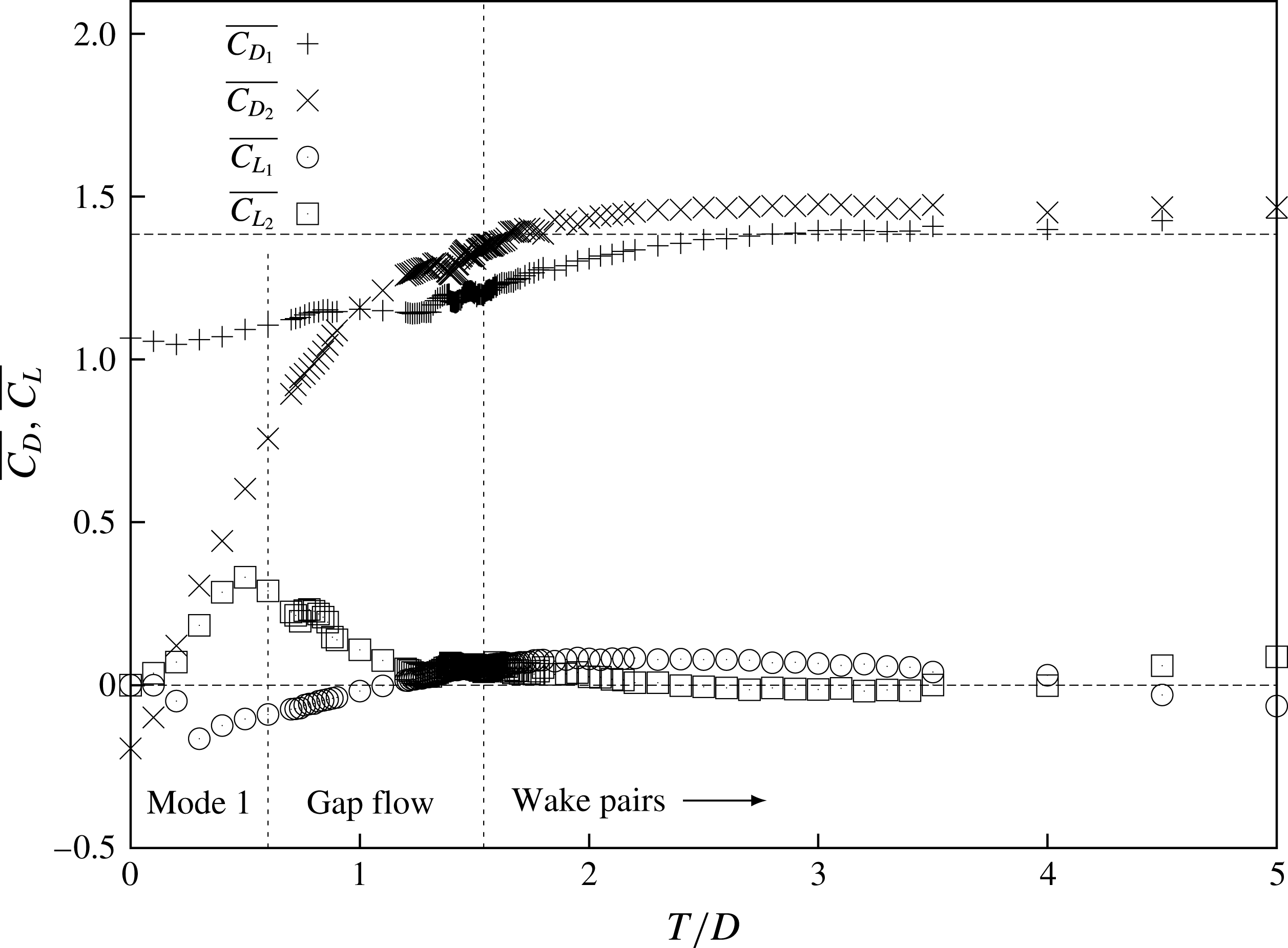
Figure 9 plots the variation with cross-stream offset of the mean values of the lift and drag coefficients for both cylinders. For the tandem cylinders (
 $T=0.0$
), most of the drag is experienced by the front cylinder; the rear cylinder experiences a negative mean drag. The negative mean drag on the rear cylinder only occurs for offsets
 $T/D<0.2$
. The drag on the rear cylinder increases almost linearly up to offset
 $T/D=1.0$
, from which point it exceeds the drag on the front cylinder.
The mean lift force is zero for the tandem
 $T=0.0$
configuration. With increasing offset, the mean lift becomes positive for the rear cylinder and negative for the front, indicating a mean force on the cylinders away from the centreline. Around
 $T/D=1.2$
, the lift on the front cylinder becomes positive again.
Figure 9 only describes the mean forces on the cylinders. Figure 10 plots the variation with offset
 $T/D$
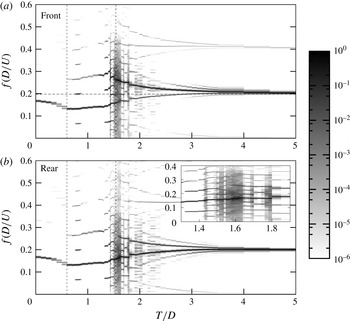
of the intensity across the spectrum frequency in the coefficient of lift signal, for both cylinders, replotting figure 6(a), but including the data for both the upstream (top) and downstream (bottom) cylinders. The primary frequency of the vortex shedding in each case can be identified by the darkest sections of the plot. Immediately apparent is that, for
 $T/D\lesssim 0.6$
(i.e. mode 1 according to figure 8), the vortex shedding frequency from both cylinders is similar, and is less than the vortex shedding (Strouhal) frequency of the single isolated cylinder,
 $St=0.198$
. This corresponds well to the first base ‘mode’ identified from previous literature and described in the introduction (§ 1), for
 $T/D\lesssim 0.4$
, where there is no gap flow between the cylinders.
For
 $L/D=1.5$
and fixed cylinders (
 $U^{\ast }=0$
), the frequency content of the lift force as a function of
 $T/D$
for both cylinders. The plots are formed in the same way as described in figure 6. The horizontal dotted line indicates the Strouhal frequency for a single isolated cylinder. Vertical dashed lines represent the boundaries between mode 1, gap flow and wake pair dominated regions, as in figure 8.

For
 $0.6\leqslant T/D\lesssim 1.5$
, figure 10 shows that the primary frequency of the flow starts to increase with increasing
 $T/D$
, and a stronger component at twice the primary frequency also appears. This corresponds to the second ‘base’ mode described in § 1 identified from the literature for
 $0.4\leqslant T/D\leqslant 1.3$
, and characterised by a flow through the gap between the cylinders that becomes stronger with increasing
 $T/D$
. The presence of a frequency at twice the primary frequency is a direct consequence of the broken symmetry due to the non-zero offset – each vortex shed in the wake has an impact on the gap flow, which induces a force in the same direction regardless of the sign of the vortex, hence the doubling of the frequency.
For
 $T/D\gtrsim 1.5$
, with the transition to a wake pair dominated flow according to figure 8, a more complex behaviour appears. This results from the presence of a difference in primary vortex shedding frequency on each cylinder, and the close proximity of these vortex wakes occurring at different time scales. Again, this is consistent with the third ‘base’ mode described from the literature for
 $T/D>1.3$
in § 1. In these cases, the upstream cylinder is now forming and shedding its own vortex pairs. These vortices have a smaller formation area because of the presence of the downstream cylinder, which results in smaller vortices being shed at a higher frequency than they do from the downstream cylinder. Figure 10 shows that the flow can be highly complex, with a frequency response consisting of a series of well-defined harmonics, or broadband noise in the range
 $1.5<T/D<1.8$
, the focus of the inset of the spectrum plot for the rear cylinder. The difference in primary frequency decreases with increasing
 $T/D$
, until they both converge to the value for a single cylinder at large values of
 $T/D$
. The phenomenon of different Strouhal frequencies has also been noted in Alam & Sakamoto (Reference Alam and Sakamoto2005), in a study of flow past staggered cylinders. For non-tandem and non-side-by-side arrangements, they observed, for a far greater Reynolds number than the current study,
 $Re=5.5\times 10^{4}$
, sometimes intermittently, different Strouhal frequencies for particular cases, describing the flow as bi- or multistable.
This range of cross-stream offset
 $0.0\leqslant T/D\leqslant 5.0$
was also covered numerically in the work of Tong, Cheng & Zhao (Reference Tong, Cheng and Zhao2015) for
 $Re=10^{3}$
, but traversed in terms of angle and pitch ratio between the two cylinders (see their figure 4). The description of the regimes provided here is consistent with their figure 18 along a traverse at
 $L/D=1.5$
.
For stationary cylinders,
 $U^{\ast }=0$
, plots of vorticity contours, time series of the coefficient of lift of each cylinder and the corresponding spectra, red corresponding to the upstream cylinder and green the downstream, for cylinder offsets
 $T/D=0.0$
,
 $1.0$
,
 $2.3$
and
 $3.5$
. Contours vary from blue to red in the range
 $-1\leqslant \unicode[STIX]{x1D714}_{z}D/U\leqslant 1$
.

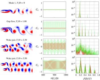
Figure 11 plots details of four cases, picking out the various regimes of behaviour classified in figure 8 and further described in figures 9 and 10. The flows for offset
 $T/D=0.0$
correspond to mode 1 where the front cylinder does not shed vortices and only one vortex street is present. Offset
 $T/D=1.0$
however corresponds to the gap-dominated flow regime and the flow is more complex with stronger contributions from all harmonics of the primary frequency present in the lift coefficient signal of each cylinder. Despite the gap flow, the cylinders still largely shed vortices as one body. In both cases the vortex formation region is larger than for the single isolated cylinder, resulting in a lower vortex shedding frequency. For
 $T/D=2.3$
, the flow is now wake pair dominated. A periodic beating is evident in the time series of the cylinder oscillation, indicative of the difference in primary vortex shedding frequency. For the case of
 $T/D=3.50$
, the frequency difference persists, but is much smaller, resulting in a weaker, longer-period beating in the signal as the interaction between the wakes lessens as the cylinders are moved further apart.
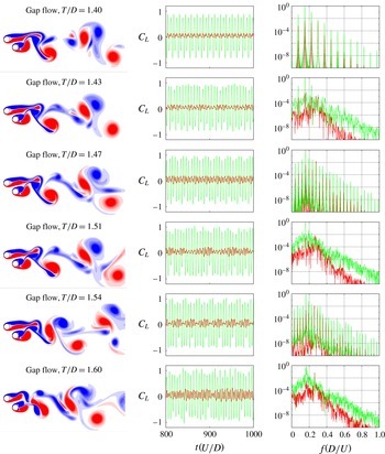
Figure 12 focuses on cases where there is a significant difference between the primary frequencies, spanning the range
 $1.3\leqslant T/D\leqslant 1.9$
, the same range as shown in the inset in figure 10. This range encompasses the transition from gap pair dominated to wake pair dominated flow. The inset shows a frequency content strongly dependent on cross-stream offset. Data have been obtained at a high resolution of
 $T/D$
, and figure 12 presents six example flows in this region. Figure 12 shows the complexity of the wake and the subtle shifts that can occur with small changes in the offset, as the flow generated through the gap between the cylinders is highly sensitive.
For stationary cylinders,
 $U^{\ast }=0$
, plots of vorticity contours, time series of the coefficient of lift of each cylinder and the corresponding spectra, red corresponding to the upstream cylinder and green the downstream, for cylinder offsets
 $T/D=1.40$
,
 $1.43$
,
 $1.47$
,
 $1.51$
,
 $1.54$
and
 $1.60$
. Contours vary from blue to red in the range
 $-1\leqslant \unicode[STIX]{x1D714}_{z}D/U\leqslant 1$
.

The images of the flow are all taken at a similar phase, when the lift force is at a local maximum. The images show that the large-scale features of the wake are not impacted greatly by the small change in offset. However, the associated time series of lift force, and the resulting frequency spectra, show very strong variation driven by the complex flow in the gap. For example, each second case shown (offsets,
 $T/D=1.43,1.51$
and
 $1.60$
) are P
 $_{N}$
-periodic, repeating over
 $N$
vortex shedding cycles (where
 $N=2,4,5$
, respectively). This is indicated by the regular modulation of the time series of the lift force and the ‘comb’ structure of the frequency spectra, with frequencies occurring at increments that are
 $f/N$
, where
 $f$
is the vortex shedding frequency. In fact,
 $N$
can be discerned by counting how many spikes occur in the spectrum before the primary frequency. The shedding locks on to these P
 $_{N}$
oscillations for extremely narrow ranges of cross-stream offset. These periodic cases are interleaved with quasi-periodic or even chaotic responses at offsets
 $T/D=1.40,1.47,1.54$
. In these cases, the modulation in the time series is less regular, and the frequency spectra are more broadband, with an essentially continuous distribution of energy across frequencies. This interleaving of P
 $_{N}$
-periodic with quasi-periodic and chaotic responses leads to an incredibly dense variation of frequency content (see the inset of figure 10). Such a dense variation does not seem to persist for the vibrating cylinders (see figure 6), or for the qualitatively similar
 $U^{\ast }=14.0$
case; in these cases the cylinders are not rigidly held and hence the vortex shedding frequencies are not rigidly tuned to the cross-stream offset.
5.3 The
$T/D=0$
limiting case: tandem cylinders

This section examines the case of vibrating cylinders aligned in a tandem configuration,
 $T/D=0$
; from figure 8 traversing the bottom edge of the parameter space. Borazjani & Sotiropoulos (Reference Borazjani and Sotiropoulos2009) presented results for this
 $T=0.0$
and
 $L/D=1.5$
case, for the reduced velocity range
 $3\leqslant U^{\ast }\leqslant 14$
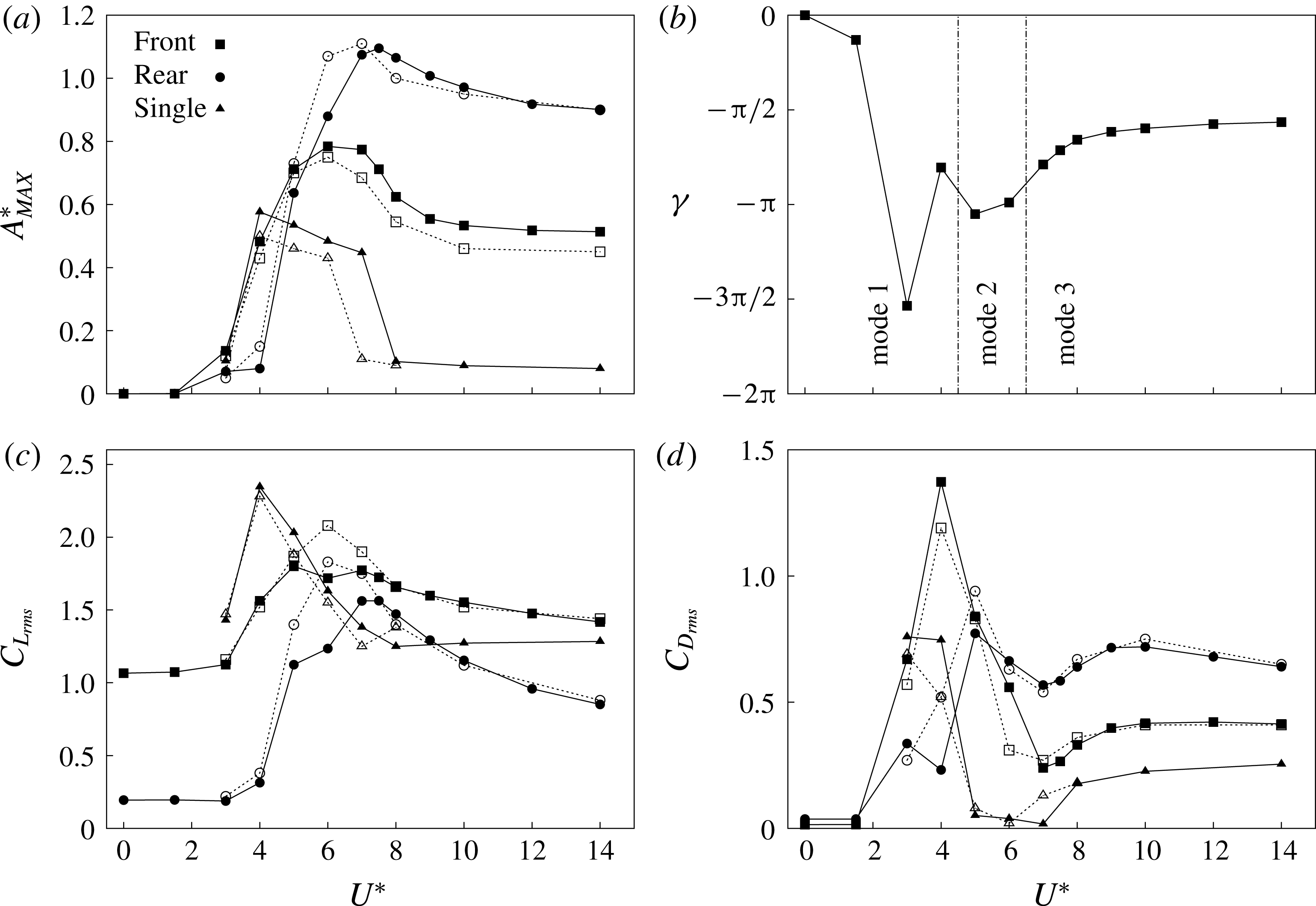
. That work is compared and expanded on in this section. Figure 13 plots a direct comparison of the slice of the parameter space of the current study, at
 $T/D=0.0$
, with the work of Borazjani & Sotiropoulos (Reference Borazjani and Sotiropoulos2009), showing the variation of maximum displacement, and of r.m.s. values of the coefficients of drag and lift for each cylinder. Also shown are comparison data of a single isolated vibrating cylinder from both the current study and Borazjani & Sotiropoulos (Reference Borazjani and Sotiropoulos2009). The
 $A_{MAX}^{\ast }$
value is calculated as the mean of the greatest 10 % of local peaks of
 $Y$
. The general picture given by the current results and those of Borazjani & Sotiropoulos (Reference Borazjani and Sotiropoulos2009) is the same across the three scalars presented in figure 13, providing a level of confidence in the results obtained. However, there are some differences that need to be addressed. For the single isolated cylinder, the values of
 $A_{MAX}^{\ast }$
for the range
 $4\leqslant U^{\ast }\leqslant 7$
, for the current study, are greater than those from Borazjani & Sotiropoulos (Reference Borazjani and Sotiropoulos2009). For the tandem arrangement, the oscillation amplitude of the front cylinder is greater, while that of the rear cylinder is reduced slightly for
 $5\leqslant U^{\ast }\leqslant 7$
. Similarly for the lift and drag, some variation between the present results and those of Borazjani & Sotiropoulos (Reference Borazjani and Sotiropoulos2009) can be seen.
For
 $T/D=0.0$
and
 $L/D=1.5$
, the variation with
 $U^{\ast }$
of the maximum displacement of each cylinder,
 $A_{MAX}^{\ast }$
, the phase difference between the cylinder oscillations,
 $\unicode[STIX]{x1D6FE}$
, and the r.m.s. values of the drag and lift coefficients. Solid symbols represent results from the current study, while hollow ones are from Borazjani & Sotiropoulos (Reference Borazjani and Sotiropoulos2009).

Attempts to eliminate this variation by trying to match the numerical set-up between the two studies were made. Borazjani & Sotiropoulos (Reference Borazjani and Sotiropoulos2009) used an inlet length and lateral clearance of
 $8D$
and an outlet length of
 $24D$
. Therefore, there is a significant difference in blockage ratio between the two studies: for a single cylinder, 6.25 % against 3.33 % for the current study. The code for the current study, run on this restricted domain, produced only marginal differences in the returned results for
 $A_{MAX}^{\ast }$
. There is also a significant difference in time step used between the two studies:
 $\unicode[STIX]{x1D6FF}t=0.02$
in Borazjani & Sotiropoulos (Reference Borazjani and Sotiropoulos2009) and
 $\unicode[STIX]{x1D6FF}t=0.004$
in the current. This difference is mostly due to the higher grid resolution used in the current study. To examine the effect of time step, we have also run both grid domain sizes using time steps of
 $\unicode[STIX]{x1D6FF}t=0.004$
and
 $0.002$
, to examine any sensitivity to temporal resolution. We found no significant effect resulting from this change in time step. We ran further tests at lower grid resolution and larger time step; the results for
 $A_{MAX}^{\ast }$
returned by the
 $M8$
grid for a time step up to
 $\unicode[STIX]{x1D6FF}t=0.0125$
were greater than those returned for the higher-resolution grid. The loose coupling scheme outlined in Borazjani & Sotiropoulos (Reference Borazjani and Sotiropoulos2009) was also implemented in the current code, but had negligible effect on the results. In short, it is not completely clear why this discrepancy exists. We note that the single cylinder results from the current study match very closely with the numerical results from Leontini et al. (Reference Leontini, Thompson and Hourigan2006) (see Griffith et al.
Reference Griffith, Lo Jacono, Sheridan and Leontini2016), which employed a highly accurate spectral-element method.
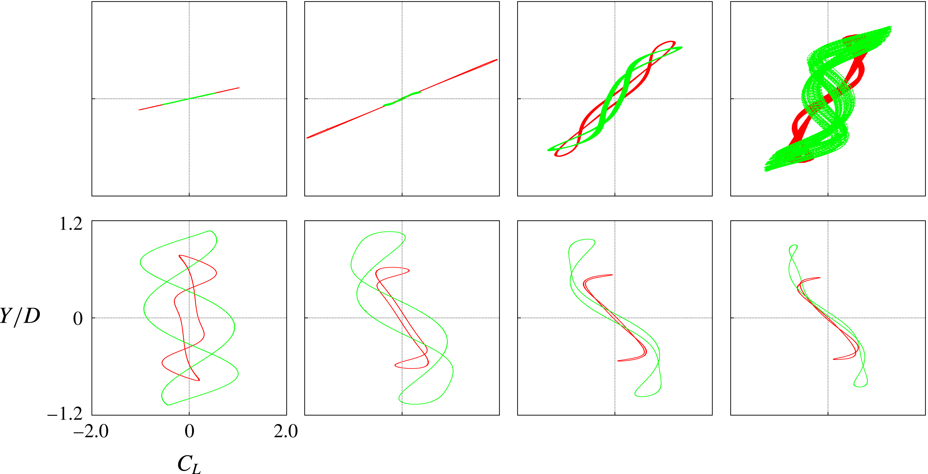
Figure 14 plots Lissajous curves of lift coefficient and displacement across the
 $U^{\ast }$
range. These curves show a strong similarity to those of figure 8 of Borazjani & Sotiropoulos (Reference Borazjani and Sotiropoulos2009). The main differences here are that the orbits are much closer to symmetric around
 $Y=0$
and
 $C_{L}=0$
in the current results (which may account for some of the differences between the two studies) and also the more meandering paths of the cases for
 $U^{\ast }=5$
and
 $6$
, indicative of some quasi-periodicity.
For the tandem arrangement with zero offset
 $T/D=0.0$
, Lissajous curves of lift coefficient and displacement for
 $U^{\ast }=3$
,
 $4$
,
 $5$
,
 $6$
,
 $7$
,
 $8$
,
 $10$
and
 $14$
. Red represents the front cylinder and green the rear cylinder.

It is shown below that these cases,
 $U^{\ast }=5$
and
 $6$
, occur in a distinct shedding regime where vortices formed at the rear of the front cylinder are forced through the gap between the cylinders to one side of the rear cylinder at one point in the oscillation cycle, and then to the other side of the rear cylinder a half-cycle later, as the two cylinders oscillate essentially out of phase. The result of this is that the lift forces on, and the resulting motions of, the two cylinders come from complex vortex–vortex and vortex–structure interactions, similar to the classic wake-induced vibration description provided in Assi et al. (Reference Assi, Bearman and Meneghini2010). Hence, it is probably unsurprising that there is not an exact match between the two studies for these cases.
For zero cross-stream offset,
 $T/D=0.0$
, Borazjani & Sotiropoulos (Reference Borazjani and Sotiropoulos2009) defined two broad flow states: state 1 refers to those cases where the front cylinder oscillates with larger amplitude than the rear, for
 $U^{\ast }\leqslant 4.0$
; state 2, where the rear cylinder oscillates with larger amplitude, for
 $U^{\ast }\geqslant \approx 7.0$
. They classed the cases in between these two ranges as ‘critical’ cases in the transition between the two states. Using the vortex shedding pattern classification of Williamson & Roshko (Reference Williamson and Roshko1988), state 1 consists of a 2S vortex shedding pattern, where a single vortex of each sign is shed from the rear cylinder, with the rear cylinder enveloped by shear layers beginning at the front cylinder. State 2 consists of a 2P vortex shedding pattern, with vortices of each sign shed from both cylinders with complex vortex interaction and merging in the near wake. The ‘critical’ case for
 $U^{\ast }=5.0$
shows similarity to state 2, but does not show a 2P ordering, with complex interactions resulting from fast-moving vortices merging with earlier-shed vortices, producing a less ordered wake.
As outlined in the discussion of figure 8, it is proposed that the two states described by Borazjani & Sotiropoulos (Reference Borazjani and Sotiropoulos2009) are better described as regimes or modes and that the ‘critical’ cases (
 $U^{\ast }=5.0$
and
 $6.0$
) are in fact a distinct mode, rather than a transition case. The distinctions can be observed in the different
 $Y{-}C_{L}$
orbits of figure 14 and the similarities between the orbits within the ranges of
 $U^{\ast }$
just described.
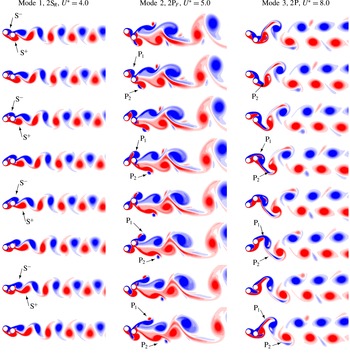
Plots of vorticity contours throughout the oscillation for representative cases of each of the three modes are shown in figure 15. For mode 1 cases, shown for
 $U^{\ast }=4.0$
, the rear cylinder sits in the wake of the front cylinder throughout the oscillation cycle. The oscillation of the rear cylinder is small compared to the front cylinder (see figure 13). Vorticity that forms on the front cylinder merges with vorticity of the same sign on the rear cylinder. Vortices are shed only from the rear cylinder. One vortex of each sign is shed in each cycle, forming a regular vortex street. Given that the vortices are shed from the rear cylinder, we denote the shedding mode as 2S
 $_{R}$
. The mode exists for cases of
 $U^{\ast }=3.0$
and
 $U^{\ast }=4.0$
, with simulations requiring long run times (
 $750U^{\ast }$
) to reach a statistically converged solution.
For the tandem cylinder arrangement (
 $T/D=0.0$
), vorticity contours for three cases,
 $U^{\ast }=4.0$
,
 $5.0$
and
 $8.0$
, describing the three vortex shedding modes, 2S
 $_{R}$
, 2P
 $_{F}$
and 2P. Each series of images depicts an oscillation cycle of the primary frequency, beginning with the front cylinder at its maximum displacement. Contours vary from blue to red in the range
 $-1\leqslant \unicode[STIX]{x1D714}_{z}D/U\leqslant 1$
.

For
 $U^{\ast }=5.0$
and
 $6.0$
, the rear cylinder oscillates more, coming out fully from behind the front cylinder. The cylinders oscillate out of phase,
 $\unicode[STIX]{x1D6FE}=\unicode[STIX]{x03C0}$
(see figure 13). In contrast to mode 1, vortices do not form on the rear cylinder; instead only a small amount of vorticity is deposited in a trail. A vortex pair forms in the (periodically) larger space now available between the cylinders. This larger space is now available due to the elastic mounting of the springs, despite the close proximity of the cylinders (
 $L/D=1.5$
). This large space allows the formation of vortices in the gap, creating a wake-induced vibration on the rear cylinder (Assi et al.
Reference Assi, Bearman and Meneghini2010). As the vortex pair forms, it is cut off by the rear cylinder, its orientation rolling (see P
 $_{1}$
in the second to fourth images of figure 15), before meeting free-stream fluid and convecting at high velocity downstream (P
 $_{1}$
in the fifth to eight images of figure 15). The vortex pairs overtake earlier pairs, merge and form an irregular vortex street. Because of the two vortex pairs formed in each cycle, which mostly form on the front cylinder, we denote this shedding mode 2P
 $_{F}$
. Apparent in the contour fields, plotted over one period of the dominant frequency, there is some quasi-periodicity; tracking down the images from top to bottom, one can see that the topology of the vorticity field is not going to repeat in the next period. For that reason, we denote this case as the period-doubling oscillation case on figure 7.
Mode 3 exists for
 $U^{\ast }\geqslant 7.0$
and is characterised by large oscillation of the rear cylinder, with the oscillation of the rear cylinder lagging the front cylinder by
 $\unicode[STIX]{x1D6FE}\simeq \unicode[STIX]{x03C0}/2$
. Similar to mode 2, the rear cylinder traverses the wake of the front, but, instead of a vortex pair forming in the gap, the rear cylinder effectively cuts through the shear layers of the front cylinder (the third to fifth images of figure 15). In a complex interaction, negative and positive vorticity from the front cylinder is subsumed by the vortex formation on the rear cylinder each half cycle. Each cycle, this vortex mingling creates two pairs of unequal-strength vortices. To account for the complex formation of these vortex pairs, the shedding mode is denoted as a 2P. These three vortex shedding modes cover the
 $T=0.0$
parameter space. The next section will examine the effect of increasing a cross-stream offset, introducing the staggered vibrating cylinder arrangement.
5.4 Variation of cross-stream offset
$T/D$

This section describes example cases from the
 $U^{\ast }$
–
 $T/D$
parameter space not contained along the
 $U^{\ast }=0.0$
and
 $T/D=0.0$
axes. On figure 8, the tandem modes (modes 1, 2 and 3) are marked on and near the
 $T/D=0.0$
axis. As the cross-stream offset increases, mode 1, featuring vortex shedding from the rear cylinder only, persists up until
 $T/D=0.6$
, when gap flow dominated flows appear. For modes 2 and 3, for increasing offset, these first give way to modes
 $2_{1}$
and
 $3_{1}$
, which are essentially one-sided versions of the tandem modes 2 and 3.
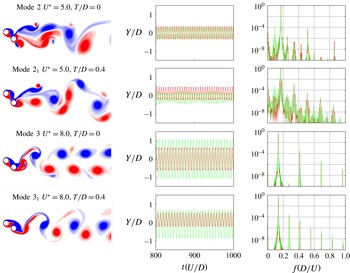
Figure 16 plots four cases, showing examples of the tandem modes 2 and 3 and the one-sided, or asymmetric, versions of these modes. In this figure, the period doubling of modes 2 and
 $2_{1}$
is evident in the presence of energy at a frequency of half the primary frequency. Mode
 $2_{1}$
differs from mode
 $2$
, in that the vortex pairs in the wake (labelled in the bottom panel of the example in figure 15) are only shed from the upstream cylinder; similarly, the rolling of the vortex pair in the gap identified for mode
 $2$
only occurs on one side of the cylinders. The resultant wake mode is a P
 $_{F}$
+S
 $_{R}$
, with a single vortex shed from the downstream cylinder and a pair from the front. Similarly, the shear layer cut-through that occurs for mode
 $3$
only occurs on one side of the cylinders for mode
 $3_{1}$
. This results in a periodic P+S wake for mode
 $3_{1}$
, rather than the periodic 2P wake for mode 3.
For
 $U^{\ast }=5.0$
and
 $8.0$
, and
 $T/D=0.0$
and
 $0.4$
, plots of vorticity contours, time series of the displacement of each cylinder and the corresponding spectra for the displacements; red corresponding to the upstream cylinder and green the downstream. These four cases give examples, top to bottom, of the modes 2,
 $2_{1}$
, 3 and
 $3_{1}$
, as shown on figure 8. Contours vary from blue to red in the range
 $-1\leqslant \unicode[STIX]{x1D714}_{z}D/U\leqslant 1$
.

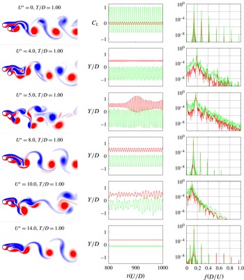
Moving further in the higher offset direction of the parameter space depicted in figure 8, a region labelled ‘Gap flow dominated’ is encountered, centred around a cross-stream offset of
 $T/D=1.0$
. Figure 17 presents six cases in this region, for a cross-stream offset of
 $T/D=1.0$
, for values of
 $U^{\ast }=0.0$
, 4.0, 5.0, 8.0, 10.0 and 14.0. These are cylinder configuration for which the gap flow is the predominant feature of the flow; this implies an interaction of either shear layers or vortices emanating or forming on the inside sides of the cylinders. These are shear layers and vortices formed on different cylinders, having different formation areas and exposure to the oncoming free stream. There are no pairs of alternating vortices being shed from one cylinder at a given frequency; there are several frequencies possible, tied to vortex and vorticity formation on both sides of both cylinders. Therefore, this region features both periodic flows and flows characterised by quasi-periodicity and disordered vortex shedding.
For
 $T/D=1.0$
, plots of vorticity contours, time series of the displacement of each cylinder and the corresponding spectra for the displacements, red corresponding to the upstream cylinder and green the downstream, for reduced velocities,
 $U^{\ast }=0.0$
,
 $4.0$
,
 $5.0$
,
 $8.0$
,
 $10.0$
and
 $14.0$
. These six cases give examples of the gap flow dominated region of figure 8. Contours vary from blue to red in the range
 $-1\leqslant \unicode[STIX]{x1D714}_{z}D/U\leqslant 1$
.

From figure 17, the common feature of the cases shown is the gap flow. In all cases, the positive vorticity generated from the upstream cylinder completely or substantially passes through the gap between the two cylinders. Following on from this is an interaction or pairing of the shear layers and vortices on the inside sides of the two cylinders; together with the elastic mountings of the cylinders, the combination of several unrelated frequencies results in the quasi-periodic flows seen for the reduced velocity cases
 $U^{\ast }=4.0$
,
 $5.0$
and
 $10.0$
from figure 17. The case shown for
 $U^{\ast }=5.0$
exhibits a strong intermittency indicative of a chaotic flow.
A distinction needs to be drawn between these gap flow dominated cases and the tandem modes 2 and 3. The tandem modes also feature strong gap flow, but the gap is present due to the elasticity of the cylinder mountings (
 $U^{\ast }$
) – and can therefore change sides – rather than the initial position of the cylinders (
 $T/D$
). Therefore, the ‘Gap flow dominated’ region can extend over the entire range of
 $U^{\ast }$
.
Increasing the cross-stream offset, the region marked ‘Wake pair dominated’ on figure 8 covers the parameter space entirely for
 $T/D>2.0$
. In this region, instead of being determined by the interaction of vorticity in the gap, the flow is dominated by pairing of vortices shed from one cylinder. Figure 18 presents flows for the same reduced velocities as in figure 17, but for a cross-stream offset of
 $T/D=3.0$
. All of the flows are in the ‘Wake pair dominated’ region. Although mixing of vortex streets can occur in the far wake (see the vorticity snapshots for
 $U^{\ast }=4.0$
and
 $5.0$
), the cylinder oscillations are determined by the pairing and interaction of the vortices formed on each cylinder. This distinguishes the categorisation from the T-I and T-II regimes described by Hu & Zhou (Reference Hu and Zhou2008) and used by Tong et al. (Reference Tong, Cheng and Zhao2015), which delineate the flow according to vortex interactions at six cylinder diameters downstream. The ‘Wake flow dominated’ categorisation refers to the forcing on the cylinder and hence on the near wake. In the cases shown in figure 18, the vorticity topology in the near wake is clearly defined by the wake pairs shed from each single cylinder.
For
 $T/D=3.0$
, plots of vorticity contours, time series of the displacement of each cylinder and the corresponding spectra for the displacements, red corresponding to the upstream cylinder and green the downstream, for reduced velocities,
 $U^{\ast }=0.0$
,
 $4.0$
,
 $5.0$
,
 $8.0$
,
 $10.0$
and
 $14.0$
. These six cases give examples of the wake pair dominated region of figure 8. Contours vary from blue to red in the range
 $-\!1\!\leqslant \unicode[STIX]{x1D714}_{z}D/U\leqslant 1$
.

For all six cases, the vortices appear organised. However, only the cases for reduced velocity
 $U^{\ast }=4.0$
and
 $5.0$
are classified as periodic, as shown on figure 7. For these two cases, the cylinders oscillate at the same primary frequency, with significant amplitude. For reduced velocities
 $U^{\ast }=0.0$
,
 $8.0$
,
 $10.0$
and
 $14.0$
, the cylinders either strictly do not, or only barely, vibrate, maintaining transverse separation between the cylinders. In each case, the cylinder oscillations are not synchronised, with small differences between the primary frequencies of the two cylinders resulting from the weak, but still present and noticeable, effect of the cylinders on each other; these cases are therefore classed as quasi-periodic. The small difference in frequency can be discerned in the time series of the lift coefficient shown for the
 $U^{\ast }=0.0$
case, producing a corresponding long period (approximately
 $50$
time units) beating. At this point the separation between the cylinders is such that they are approaching the state of a single isolated cylinder, which for these reduced velocities results in quasi-periodic oscillation, due to the non-matching Strouhal frequency and structural frequency.
The distribution across the parameter space of the cases featuring periodic oscillations with the same primary frequency is interesting. For the cases where the structural frequency is close to the Strouhal frequency (reduced velocity
 $U^{\ast }=5.0$
), single-harmonic periodic oscillation occurs only for high cross-stream offset, as it does for the single isolated cylinder. In contrast, for the tandem cases, the flow is characterised by period multiplying and quasi-periodicity for the reduced velocity range
 $4.0\leqslant U^{\ast }\leqslant 6.0$
. It is only outside of this range (which gives quasi-periodicity for the single cylinder vibration) that periodic flow occurs for the tandem, or almost tandem, configuration.
6 Validity of the current work
The direct numerical simulations of this study are all two-dimensional, and at
 $Re=200$
. There is strong evidence to suggest that these flows will be essentially two-dimensional at this
 $Re$
. The transition to three-dimensional flow for a single rigidly mounted cylinder occurs at
 $Re\simeq 190$
(Williamson Reference Williamson1988; Barkley & Henderson Reference Barkley and Henderson1996). However, it has been shown that transverse oscillation can delay this transition to
 $Re\simeq 280$
(Leontini, Thompson & Hourigan Reference Leontini, Thompson and Hourigan2007). Also, the transition to three-dimensional flow occurs at higher
 $Re$
for two rigidly mounted tandem cylinders, becoming higher as the cylinder spacing becomes shorter. At a spacing of
 $L/D=3.5$
, this transition is delayed to
 $Re=250$
(Deng et al.
Reference Deng, Ren, Zou and Shao2006). However, without further stability analysis, three-dimensional simulation, or experiments, it cannot be absolutely ruled out that some of these flows may be three-dimensional.
How much impact the development of three-dimensional structure has at
 $Re=200$
, or as the Reynolds number is further increased, is not clear. For the related problem of two tandem, rigidly mounted cylinders, the Reynolds number seems to have little impact on critical spacings for the development of vortex shedding regimes, and the frequency of this vortex shedding. However, the magnitudes of the induced forces are certain to be
 $Re$
-dependent, which will impact the dynamic response. For a single elastically mounted cylinder, the Reynolds number has a strong influence on the amplitude of vibration and the character of the vibration (Raghavan & Bernitsas Reference Raghavan and Bernitsas2011), and it seems likely that this will also be the case in the multi-cylinder problem. Assessing this impact is left to future work.
7 Conclusions
This study has detailed the dynamic response of two identical elastically mounted cylinders placed in tandem and staggered arrangements in a free-stream flow at Reynolds number 200. The streamwise separation of the cylinders was held constant at
 $L/D=1.5$
. The parameter space investigated spanned: the range of cross-stream offset
 $0.0\leqslant T/D\leqslant 5.0$
, from tandem arrangement, through staggered, to nearly isolated; and reduced velocity
 $0.0\leqslant U^{\ast }\leqslant 14.0$
, from rigid, stationary cylinders through to cylinders mounted on slack springs.
It is shown that the main distinguishing feature between different modes of response is the existence and influence of a significant flow through the gap between the cylinders. For the elastically mounted cylinders, this gap flow can be dynamic, as the direction of the flow through the gap switches as the relative position of the cylinders changes as they oscillate. A map of regimes was provided, detailing major vortex shedding modes. The temporal quality for the flow was also classified. These temporal classifications were then used to further decompose the major modes into periodic and non-periodic modes. It is shown that, unlike a single cylinder, matching the natural frequency of the two cylinders to the vortex shedding frequency of a single cylinder does not result in synchronised oscillations, but instead generates quasi-periodicity and chaos.
For rigid cylinders (
 $U^{\ast }=0.0$
), three base modes were identified from the literature and confirmed via simulations, corresponding to no gap flow, gap pair dominated and wake pair dominated flows with increasing offset. However, for offsets close to the gap pair/wake pair transition (around
 $T/D=1.5$
), complicated P
 $_{N}$
-periodic, quasi-periodic and chaotic flows are generated.
On the other axis of the parameter space,
 $T/D=0.0$
, a new description of the oscillations was presented, describing three modes differentiated by oscillation amplitudes, oscillation phase difference and gap flow vortex dynamics. Mode 1, for
 $0.0\leqslant U^{\ast }<4.5$
, involves small, or no, oscillation and vortices shed from the rear cylinder only. Mode 2, for
 $4.5\leqslant U^{\ast }<6.5$
, produces greater-amplitude out-of-phase oscillation, producing a periodically larger gap between the cylinders. Vortex pairs from the front cylinder travel and roll through the gap, producing a period-multiplying 2P
 $_{F}$
wake. Mode 3, for
 $U^{\ast }\geqslant 6.5$
, produces the largest oscillation. It involves the rear cylinder ‘chasing’ the front, lagging by a quarter of a period. Vorticity from the front cylinder combines with vorticity from the rear to shed vortices from the rear cylinder only, producing a 2P wake. Modes 2 and 3 feature significant periodic gap flow, with the gap resulting from the elastic cylinder mountings.
Moving away from the tandem configuration, modes
 $2_{1}$
and
 $3_{1}$
occur, essentially one-sided versions of the tandem modes 2 and 3. Around
 $T/D=1.0$
, the flow is dominated by the gap flow, with the gap between the cylinders determined principally by the initial cross-stream offset. Here, the gap flow results in shear layers and vortices shed from the inside sides of the cylinders. This leads to smaller-amplitude, quasi-periodic and chaotic oscillation. Beyond
 $T/D=2.0$
, the flow is dominated by vortex pairs shed from each cylinder, converging towards the behaviours of a single isolated cylinder for the given reduced velocity.
Acknowledgements
This work was financially supported by the Australian Research Council (ARC) Discovery Project scheme through grant number DP150103177, and the Centre National de la Recherche Scientifique (CNRS) PICS grant CLEAN-FIV. Computations were conducted using the facilities of the National Computational Infrastructure (NCI) through competitive grant IZ4, and the facilities of the Swinburne University Centre for Astrophysics and Supercomputing.