1 Introduction
Oceanographic observations show that islands might be surrounded by closed flows. Near-shore circulation was found around the Hawaiian islands (Patzert & Wyrtki Reference Patzert and Wyrtki1974), as well as around Iceland, Taiwan, the islands of Kuril Chain (Shtokman Reference Shtokman1966) and the Pribilof islands (Kowalik & Stabeno Reference Kowalik and Stabeno1999). Longuet-Higgins (Reference Longuet-Higgins1967, Reference Longuet-Higgins1969, Reference Longuet-Higgins1970) suggested that closed mass-transporting currents around islands might be induced by inertial and subinertial oscillations and probably reinforced by waves trapped by the sloping topography (see also Brink (Reference Brink1999) and Dyke (Reference Dyke2005)). He noted that the current near the island of Bermuda (Stommel Reference Stommel1954) can be attributed to this effect. Shtokman (Reference Shtokman1966) suggested that the currents around islands may be generated by wind fields in the islands’ vicinity (see also Patzert & Wyrtki Reference Patzert and Wyrtki1974). In this paper we study the conditions for barotropic instability of such flows in an idealized model, with the emphasis on the bottom-topography effect.
Pingree & Maddock (Reference Pingree and Maddock1980, Reference Pingree and Maddock1985) demonstrated numerically the possibility for existence of closed flows around islands. They found that nonlinear effects of advection and stretching of an oscillating vorticity field around a circular island give rise to a residual (after tides) circular flow. They used the rotating shallow-water model with frictional drag from the bottom, and the condition of zero vorticity at the coastal boundary (to ensure no vorticity generation there). The residual flow was calculated numerically; its azimuthal velocity profile was found to reach a maximum at the distance from the origin, which is approximately twice the island’s radius; at the rigid boundary the velocity was nearly zero. Accordingly, the vorticity changed sign, so the flow could be viewed as composed of (at least) two vorticity rings.
The investigation of instability of inviscid two-dimensional horizontal parallel flows may be dated back to Rayleigh (Reference Rayleigh1880), who showed that a necessary condition for instability is the existence of an inflection point in the velocity profile (i.e. the existence, in a
 $y$
-dependent velocity profile
 $U$
, of a point where
 $\text{d}^{2}U/\text{d}y^{2}=0$
). Lin (Reference Lin1944) showed that the Rayleigh criterion is not a sufficient condition for instability in general, and later Fjørtoft (Reference Fjørtoft1950) showed that a necessary condition for instability of a flow with a monotonic velocity profile having one inflection point is
 $(U-U_{0})\,\text{d}^{2}U/\text{d}y^{2}\leqslant 0$
for all points in the flow, with
 $U_{0}$
being the velocity in the inflection point. Eigenvalue solutions of a large set of problems, which are related to the Rayleigh problem (comprising different basic-flow profiles and different boundary conditions), were reviewed by Drazin & Howard (Reference Drazin and Howard1966).
In the rotating shallow-water model, which is quite a general framework for the consideration of flows on a rotating planet, the potential vorticity (PV), defined as
 $(\unicode[STIX]{x1D701}+f)/h$
, is conserved; here
 $h$
is the thickness of the layer in which the flow occurs,
 $\unicode[STIX]{x1D701}$
is the vertical component of the flow velocity curl and
 $f$
is the Coriolis parameter. Under certain conditions, the PV of a barotropic flow may be represented as just a sum of the relative vorticity, which can vary in time, and a time-independent background vorticity. In the presence of a gradient of the background vorticity, Rossby waves may exist. There are three main sources for the emergence of a background vorticity gradient in barotropic geophysical flows. The first is the south–north gradient
 $\unicode[STIX]{x1D6FD}$
in the Coriolis parameter. In this case, assuming
 $h=\text{const.}$
and
 $\unicode[STIX]{x1D6FD}=\text{const.}$
, the PV may be redefined as
 $\unicode[STIX]{x1D701}+\unicode[STIX]{x1D6FD}y$
, where
 $y$
is the northward coordinate. This is the planetary beta-plane approximation conventionally used for qualitative description of meso- and large-scale oceanic and atmospheric flows. Because the planetary
 $\unicode[STIX]{x1D6FD}$
is positive everywhere except the planet’s poles, there must be a westward component in the phase velocity of propagation of planetary Rossby waves; this is one of the facets of the planetary beta effect. The second source is the spatial gradient in the fluid-layer thickness, i.e. a sloping bottom topography. In the case of
 $f=\text{const.}$
and a weak constant bottom slope in some
 $y$
-direction (this time, it is not necessarily northward), again the PV is equal approximately to
 $\unicode[STIX]{x1D701}+\unicode[STIX]{x1D6FD}y$
, where
 $\unicode[STIX]{x1D6FD}$
can be positive or negative and is proportional to the steepness of the slope. In such a case, one may talk of a topographic beta effect. The third source is the non-uniform shear in the main, basic flow, in the situation where the development of weak perturbations imposed on the time-independent main flow is considered. The vorticity of the basic flow then acts as the background vorticity, while the vorticity of the perturbation flow plays the role of the relative vorticity. A non-uniform shear of the basic flow induces, therefore, a shear beta effect. The direction in which the Rossby waves propagate in the case of a topographic or a shear beta effect depends on the sign of the gradient of the corresponding background vorticity. Of course, superposition of the three kinds of beta effect is possible (e.g. Kizner et al.
Reference Kizner, Shteinbuch-Fridman, Makarov and Rabinovich2017).
In the presence of the beta effect, an analogue to the Rayleigh necessary condition for instability was found by Kuo (Reference Kuo1949, Reference Kuo1973). The condition for a zonal flow on the beta plane is the existence of a point, in which the derivative of the PV across the flow vanishes, i.e. where
 $\unicode[STIX]{x1D6FD}-\text{d}^{2}U/\text{d}^{2}y=0$
. It was found that the stable modes have a phase velocity which is never greater than the maximal velocity of the flow, yet can be smaller than its minimal value. In case of instability, the mode’s phase velocity is equal to the flow velocity in the extremal point. A westward jet (on a planetary beta plane) was found numerically to be more unstable than an eastward one.
Charney & Stern (Reference Charney and Stern1962) considered parallel flows with two zones of constant PV gradients. They found that, for the normal-mode instability to occur, the two values of the gradient must be opposite in sign. Bretherton (Reference Bretherton1966) showed that the instability in such flows occurs due to the interaction of two distinct Rossby waves, which develop in the two zones and propagate (relative to the flow) in opposite directions. Based on this counter-propagating Rossby-wave concept, Heifetz, Bishop & Alpert (Reference Heifetz, Bishop and Alpert1999) gave an interpretation of Rayleigh’s normal-mode analysis of the shear instability.
The effect of exponential bottom topography on the stability of a flow in a non-periodic channel was investigated by Li & McClimans (Reference Li and McClimans2000), who used the rotating shallow-water model with the rigid-lid condition. More precisely, the gradient of the layer thickness was taken to vary exponentially across the channel, and the flow velocity profile to be a cosine. Obviously, the along-channel topographic Rossby waves in such a channel propagate so that the deeper flank of the channel lies to the left of the propagation direction. Accordingly, the stability properties of a flow going in this direction, a prograde flow, might be expected to differ from those of an oppositely directed, retrograde flow. In fact, by performing linear stability analysis for along-channel modes, Li & McClimans showed that the retrograde flow is stable in a larger range of wavenumbers than the prograde flow. Poulin & Flierl (Reference Poulin and Flierl2005) dealt with a periodic channel in the rotating shallow-water model, but by applying the free-surface condition and using hyperbolic-tangent bottom topography; as the basic flow, they used the Bickley jet, which has a squared hyperbolic-secant velocity profile. Discussing the effect of bottom topography versus the flat-bottom case, they arrived at a conclusion that the chosen bottom topography stabilizes retrograde flows and, if the slope is beyond some critical value, it stabilizes retrograde flows too; a weak slope, however, has a destabilizing effect on prograde flows. As will be seen below, our findings are consistent with these results.
Axially symmetric flows that are the subject of our paper have a substantial similarity to parallel flows. Rayleigh (Reference Rayleigh1892) showed that a necessary condition for shear instability of a circular flow is similar to the criterion for parallel flows, i.e. that
 $\text{d}\unicode[STIX]{x1D701}/\text{d}r$
should change sign; here
 $\unicode[STIX]{x1D701}=1/r\,\text{d}(rV)/\text{d}r$
is the vorticity,
 $V$
is the azimuthal velocity and
 $r$
, the polar radius. Since that time a great number of publications have appeared, being devoted mostly to the stability of flows of this kind in the presence of viscosity and differential rotation (see e.g. Drazin & Reid Reference Drazin and Reid2004; Chossat & Iooss Reference Chossat and Iooss2012; Deguchi Reference Deguchi2017, and the references therein).
The problem of stability of non-viscous circular flows around a rigid boundary has features in common with that of stability of circular vortices, as indicated by Kizner et al. (Reference Kizner, Makarov, Kamp and van Heijst2013). The stability of circular barotropic isolated vortices was first considered by Michalke & Timme (Reference Michalke and Timme1967), who found that the Rayleigh criterion applied to the radial profile of velocity works also for a vortex given as a single-sign vorticity patch. The conditions for instability of vortices with stepwise vorticity profiles were established analytically by Flierl (Reference Flierl1988), and numerically by Kozlov & Makarov (Reference Kozlov and Makarov1985) and Helfrich & Send (Reference Helfrich and Send1988), who used the contour-dynamics approach suggested by Zabusky, Hughes & Roberts (Reference Zabusky, Hughes and Roberts1979). Vortex configurations, which include three contours, were investigated for stability by Carton (Reference Carton1992) and Makarov (Reference Makarov1996).
The instabilities of flows around a circular wall over a flat bottom, i.e. on the
 $f$
-plane, were investigated by Kizner et al. (Reference Kizner, Makarov, Kamp and van Heijst2013). The basic state was chosen to consist of two concentric uniform-vorticity rings, and the instability conditions were established in the parameter space spanned by the rings’ radii. Here we follow this path, but extend the research by incorporating the effect of weak conical bottom slope on the stability of a flow around an island. With the account of the conical topographic beta effect, for a basic state, we consider an axially symmetric flow with two uniform-PV rings next to an upright rigid cylinder, and with zero velocity outside the rings. The eigenvalue equation for the complex frequency of an azimuthal-mode perturbation is derived analytically. However, as distinct from the flat-bottom case, due to the conical beta effect, the equation becomes transcendental and, therefore, is solved numerically for varying parameters of the flow. The case of an infinitesimally small slope is considered analytically.
As a first major novelty relative to the flat-bottom case, we show analytically that even weak topographic slope may generate instability in the circumstances where a flat-bottom flow is stable. Then the stability diagrams and growth rates for steeper slopes are presented and discussed. We show how the beta effect leads to a bifurcation from stability to instability even for weak slopes under certain conditions on the initial flow. For example, mode 1 in the flat-bottom case is known to be always stable (Kizner et al. Reference Kizner, Makarov, Kamp and van Heijst2013). Now we prove that the conical beta effect gives rise to the mode-1 instability; the instability takes place, however, only in clockwise flows. We discuss the bifurcation of mode 1 from stability to instability in terms of Rossby waves running at the contours of discontinuity of the basic PV and outside of the uniform-PV rings.
2 Topographic beta cone: governing equations
We consider a barotropic quasigeostrophic flow around a cylindrical island, assuming the bottom topography to be, generally, non-flat and the planetary beta effect negligible. The quasigeostrophic approximation requires for its applicability that (i) the fluid rotation be fast relative to the flow considered in a co-rotating frame of reference, and (ii) the variation in the fluid-layer thickness be much smaller than the mean thickness (see e.g. Pedlosky Reference Pedlosky2013a
; Vallis Reference Vallis2017). Under these conditions, the flow is effectively two-dimensional. Thus, in the polar coordinates
 $r$
and
 $\unicode[STIX]{x1D703}$
, which we use below, the radial and azimuthal components of velocity,
 $u$
and
 $v$
, can be expressed in terms of a streamfunction
 $\unicode[STIX]{x1D6F9}$
as
 $$\begin{eqnarray}u=-\frac{1}{r}\frac{\unicode[STIX]{x2202}\unicode[STIX]{x1D6F9}}{\unicode[STIX]{x2202}\unicode[STIX]{x1D703}},\quad v=\frac{\unicode[STIX]{x2202}\unicode[STIX]{x1D6F9}}{\unicode[STIX]{x2202}r}.\end{eqnarray}$$
Geometry of the beta-cone model.
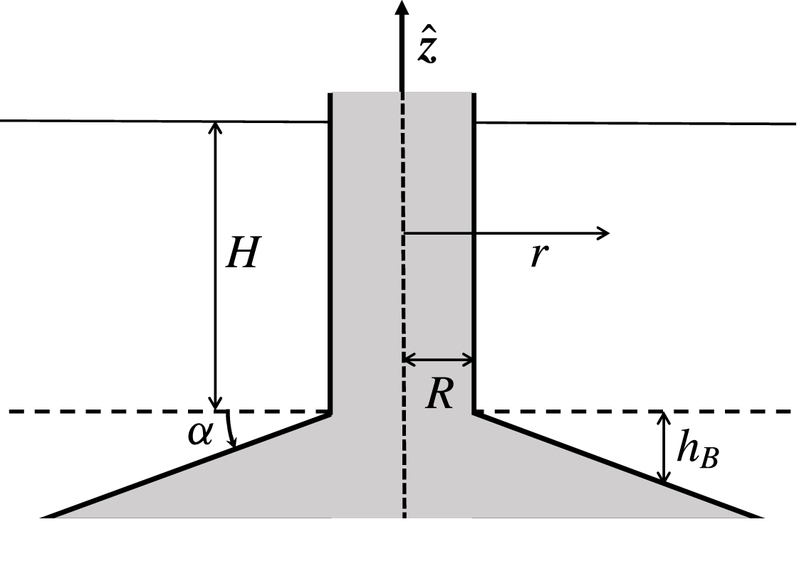
We treat the flow in a simplified geometry by regarding the island to be a circular cylinder, and the sea bottom to be a conical surface encircling the cylinder and making an angle
 $\unicode[STIX]{x1D6FC}$
with the horizontal plane. At the free surface, the rigid-lid condition is applied, so the distance
 $H$
of this boundary to the level of the cylinder–cone intersection is constant,
 $h_{B}$
denotes the deviation of the fluid-layer thickness from
 $H$
, and
 $R$
is the cylinder radius (figure 1). To guarantee the validity of the quasigeostrophic approximation, the bottom slope is assumed to be weak enough, so that
 $$\begin{eqnarray}h_{B}=(r-R)\tan (\unicode[STIX]{x1D6FC})\ll H\end{eqnarray}$$
for reasonable
 $r$
. According to condition (i) of quasigeostrophy, the relative vorticity, defined by
 $$\begin{eqnarray}\unicode[STIX]{x1D701}=\frac{1}{r}\left(\frac{\unicode[STIX]{x2202}(rv)}{\unicode[STIX]{x2202}r}-\frac{\unicode[STIX]{x2202}u}{\unicode[STIX]{x2202}\unicode[STIX]{x1D703}}\right)=\unicode[STIX]{x1D6FB}^{2}\unicode[STIX]{x1D6F9},\end{eqnarray}$$
satisfies the inequality
 $\unicode[STIX]{x1D701}\ll f$
, where
 $f=\text{const.}$
is the Coriolis parameter. Thus, the potential vorticity
 $Q$
becomes
 $$\begin{eqnarray}Q=\frac{\unicode[STIX]{x1D701}+f}{H+h_{B}}\approx \frac{1}{H}\left[\unicode[STIX]{x1D701}-\frac{f\tan (\unicode[STIX]{x1D6FC})}{H}(r-R)+f\right]=\frac{1}{H}[(\unicode[STIX]{x1D701}+\unicode[STIX]{x1D6FD}r)+(f-\unicode[STIX]{x1D6FD}R)],\end{eqnarray}$$
where
 $\unicode[STIX]{x1D6FD}=-f\tan (\unicode[STIX]{x1D6FC})/H$
is the topographic beta parameter arising from the conical bottom slope;
 $\unicode[STIX]{x1D6FD}$
is negative for a usual offshore slope in the northern hemisphere, so from now on we always take
 $\unicode[STIX]{x1D6FD}$
to be negative. Disregarding the constant term
 $f-\unicode[STIX]{x1D6FD}R$
and the factor
 $1/H$
in (2.4), we redefine the PV as
 $$\begin{eqnarray}Q=\unicode[STIX]{x1D701}+\unicode[STIX]{x1D6FD}r,\end{eqnarray}$$
i.e. the radial bottom slope induces a beta-cone effect, the background vorticity which is linear in
 $r$
. The flow is governed by the PV conservation equation:
 $$\begin{eqnarray}\frac{\unicode[STIX]{x2202}Q}{\unicode[STIX]{x2202}t}+\frac{1}{r}\left(\frac{\unicode[STIX]{x2202}\unicode[STIX]{x1D6F9}}{\unicode[STIX]{x2202}r}\frac{\unicode[STIX]{x2202}Q}{\unicode[STIX]{x2202}\unicode[STIX]{x1D703}}-\frac{\unicode[STIX]{x2202}\unicode[STIX]{x1D6F9}}{\unicode[STIX]{x2202}\unicode[STIX]{x1D703}}\frac{\unicode[STIX]{x2202}Q}{\unicode[STIX]{x2202}r}\right)=0.\end{eqnarray}$$
Strictly speaking, condition (2.2), which along with the condition
 $\unicode[STIX]{x1D701}\ll f$
underlies the quasigeostrophic approximation (2.5), breaks down at large
 $r$
. Nevertheless, in what follows, at some stages of our derivations we shall consider the limit of
 $r\rightarrow \infty$
. This is a customary practice when dealing with idealized models, such as the
 $f$
- and beta-plane approximations. In fact, when the structure and behaviour of small- and meso-scale geophysical vortices and/or Rossby waves on the unbounded
 $f$
- and/or beta plane are discussed, conditions at infinity are widely applied, despite that at infinity, the formal restrictions on which these approximations are based are not fulfilled. Experience of the use of these models shows that true limits of their applicability are often wider than the formally prescribed ones.
3 The basic flow
As noted in the Introduction, this study is an extension of the work by Kizner et al. (Reference Kizner, Makarov, Kamp and van Heijst2013), which was inspired by laboratory observations, and where the case of
 $\unicode[STIX]{x1D6FD}=0$
was explored. In laboratory conditions, whatever the reasons for the formation of a closed flow around a motionless cylinder are, molecular viscosity will cause the existence of a boundary layer, in which the velocity drops to zero at the rigid boundary. There are grounds to believe that in a two-dimensional flow, turbulent viscosity in the vicinity of a vertical cylindrical wall may play a similar role (Pedlosky Reference Pedlosky2013b
, chap. 2). Assume that the cylinder and the flow are circular and the fluid is unbounded from the outside. In a flow with the simplest structure, the velocity magnitude increases from zero at the rigid boundary to some maximum near the outer edge of the boundary layer, and then decreases to zero with increasing distance from the cylinder. Over time, in the absence of external forcing, the boundary layer expands, while the maximum velocity decreases. This process, however, is slow compared to the typical growth rate of instability, and in this sense the flow can be considered stationary.
Physically meaningful flows are flows with finite total energy, i.e. those whose velocity decreases at infinity faster than
 $1/r$
, so that the total circulation of the flow is zero. Provided that at a certain distance the velocity vanishes and remains zero up to infinity, the vorticity of the flow can be viewed as two neighbouring opposite-signed rings of finite width, with the inner ring touching the cylinder. Consider now, as an approximation, a circular flow with uniform vorticity in the rings. In a viscous fluid, a steady-state flow with such a vorticity distribution can be obtained by long-lasting rotation of a cylinder located in between two motionless cylinders co-axial with the rotating one (e.g. Landau & Lifshitz Reference Landau and Lifshitz1987, chap. II, cf. also Trieling, van Heijst & Kizner Reference Trieling, van Heijst and Kizner2010). For such a flow, the viscous terms in the Navier–Stokes equations are identically zero; therefore, the flow can be treated as a flow in an ideal fluid. The above discussion explains why, in considering a flow with a stepwise-constant vorticity profile, the condition of vanishing azimuthal velocity at the rigid boundary is only natural.
Following this path, in the presence of the beta-cone effect, for a basic state in the subsequent stability analysis we take a circularly symmetric flow with stepwise-constant PV profile around a rigid circular wall. More specifically, the wall is represented by a rigid contour
 $r=R$
, while the flow is given by two uniform-PV rings. The inner ring is bounded by the rigid contour
 $r=R$
and the liquid contour
 $r=R_{1}$
, and the outer ring is bounded by the liquid contours
 $r=R_{1}$
and
 $r=R_{2}$
, where
 $R<R_{1}<R_{2}$
. Outside the outer ring, the relative vorticity is assumed to be zero. This implies that the PV outside the outer ring is equal to
 $\unicode[STIX]{x1D6FD}r$
. Denoting the PV of the basic flow by
 $\bar{Q}$
, and the PV in the inner and outer rings by
 $\unicode[STIX]{x1D6E4}_{1}$
and
 $\unicode[STIX]{x1D6E4}_{2}$
, respectively, we write
 $$\begin{eqnarray}\bar{Q}(r)=\left\{\begin{array}{@{}ll@{}}\unicode[STIX]{x1D6E4}_{1},\quad & R\leqslant r<R_{1}\\ \unicode[STIX]{x1D6E4}_{2},\quad & R_{1}\leqslant r<R_{2}\\ \unicode[STIX]{x1D6FD}r,\quad & r\geqslant R_{2}.\end{array}\right.\end{eqnarray}$$
Thus, the gradient of the basic PV profile is
 $$\begin{eqnarray}\frac{\text{d}\bar{Q}}{\text{d}r}=(\unicode[STIX]{x1D6E4}_{2}-\unicode[STIX]{x1D6E4}_{1})\unicode[STIX]{x1D6FF}(r-R_{1})+(\unicode[STIX]{x1D6FD}R_{2}-\unicode[STIX]{x1D6E4}_{2})\unicode[STIX]{x1D6FF}(r-R_{2})+\unicode[STIX]{x1D6FD}{\mathcal{H}}(r-R_{2}),\end{eqnarray}$$
where
 $\unicode[STIX]{x1D6FF}(\cdot )$
is the Dirac delta function and
 ${\mathcal{H}}(\cdot )$
is the Heaviside function.
From this point on, we regard all the variables and constants to be non-dimensional, thus normalized, while keeping the designations unchanged. In this normalization, the radius of the rigid contour is taken as the length scale; the absolute value of PV in the inner ring, as the scale for the potential and relative vorticity, and its inverse, as the time scale. So,
 $R=1$
in non-dimensional units, but below, wherever the question of the dimensional form of the equations (especially, of the algebraic expressions in them) might arise, we shall retain the symbol
 $R$
. The non-dimensional
 $\unicode[STIX]{x1D6E4}_{1}$
can be either
 $+1$
or
 $-1$
.
According to (3.1), the PV profile (and not that of the relative vorticity) is taken stepwise constant. Nevertheless, the focus of our research is mainly on the effect of infinitesimal and small
 $\unicode[STIX]{x1D6FD}$
on the flow instability (in § 6, the case
 $\unicode[STIX]{x1D6FD}=-1$
is considered just for completeness of the presentation). Thus here, as in the flat-bottom case, the conditions of vanishing of the velocity at
 $r=R$
and
 $r\geqslant R_{2}$
are natural. Under these conditions, the velocity
 $\bar{V}(r)$
of the basic flow is calculated directly from (2.3), (2.5) and (3.1):
 $$\begin{eqnarray}\bar{V}(r)=\left\{\begin{array}{@{}ll@{}}-{\displaystyle \frac{1}{3}}\unicode[STIX]{x1D6FD}r^{2}+{\displaystyle \frac{1}{2}}\unicode[STIX]{x1D6E4}_{1}r+{\displaystyle \frac{1}{3}}{\displaystyle \frac{\unicode[STIX]{x1D6FD}R^{3}}{r}}-{\displaystyle \frac{1}{2}}{\displaystyle \frac{\unicode[STIX]{x1D6E4}_{1}R^{2}}{r}},\quad & R\leqslant r<R_{1}\\ -{\displaystyle \frac{1}{3}}\unicode[STIX]{x1D6FD}r^{2}+{\displaystyle \frac{1}{2}}\unicode[STIX]{x1D6E4}_{2}r+{\displaystyle \frac{1}{3}}{\displaystyle \frac{\unicode[STIX]{x1D6FD}R_{2}^{3}}{r}}-{\displaystyle \frac{1}{2}}{\displaystyle \frac{\unicode[STIX]{x1D6E4}_{2}R_{2}^{2}}{r}},\quad & R_{1}\leqslant r<R_{2}\\ 0,\quad & r\geqslant R_{2}.\end{array}\right.\end{eqnarray}$$
The continuity of the velocity at
 $r=R_{1}$
imposes a relation between
 $\unicode[STIX]{x1D6E4}_{1}$
and
 $\unicode[STIX]{x1D6E4}_{2}$
,
 $$\begin{eqnarray}\unicode[STIX]{x1D6E4}_{2}=-\frac{\unicode[STIX]{x1D6E4}_{1}(R_{1}^{2}-R^{2})-{\textstyle \frac{2}{3}}\unicode[STIX]{x1D6FD}(R_{2}^{3}-R^{3})}{R_{2}^{2}-R_{1}^{2}},\end{eqnarray}$$
which is equivalent to the condition of vanishing the total relative vorticity.
When
 $\unicode[STIX]{x1D6FD}=0$
, the direction of the basic flow is determined by the sign of
 $\unicode[STIX]{x1D6E4}_{1}$
; namely, the flow is counterclockwise if
 $\unicode[STIX]{x1D6E4}_{1}>0$
and clockwise if
 $\unicode[STIX]{x1D6E4}_{1}<0$
. When
 $\unicode[STIX]{x1D6FD}$
is negative but sufficiently small, the direction of the flow is still determined by the sign of
 $\unicode[STIX]{x1D6E4}_{1}$
, because according to (3.3),
 $\text{d}\bar{V}/\text{d}r|_{r=R}=\unicode[STIX]{x1D6E4}_{1}-\unicode[STIX]{x1D6FD}R$
, or what is the same,
 $\text{d}\bar{V}/\text{d}r|_{r=1}=\unicode[STIX]{x1D6E4}_{1}-\unicode[STIX]{x1D6FD}$
(once we substitute
 $R=1$
). This rule might be broken at large magnitudes of
 $\unicode[STIX]{x1D6FD}$
. In order to be able to always identify the flow direction near the cylinder by the sign of
 $\unicode[STIX]{x1D6E4}_{1}$
, in what follows we shall restrict ourselves to
 $-1\leqslant \unicode[STIX]{x1D6FD}\leqslant 0$
. This will allow us to call loosely a flow with
 $\unicode[STIX]{x1D6E4}_{1}=+1$
a counterclockwise flow, and that with
 $\unicode[STIX]{x1D6E4}_{1}=-1$
, a clockwise flow. The PV profiles defined by (3.1) may take any of the three distinct qualitative shapes shown in figure 2(a–c) along with the corresponding velocity profiles defined by (3.3).
Examples of radial profiles of the basic-flow potential vorticity
 $\bar{Q}$
(dashed, blue online) and the azimuthal velocity
 $\bar{V}$
(solid, red online) for (a)
 $\unicode[STIX]{x1D6E4}_{1}=1$
,
 $\unicode[STIX]{x1D6FD}=-0.1,R_{1}=2.5,R_{2}=4$
, (b)
 $\unicode[STIX]{x1D6E4}_{1}=-1,\unicode[STIX]{x1D6FD}=-0.1,R_{1}=2.5,R_{2}=4$
and (c)
 $\unicode[STIX]{x1D6E4}_{1}=1$
,
 $\unicode[STIX]{x1D6FD}=-0.2,R_{1}=2,R_{2}=6$
.

4 Linear stability scheme
Our aim is to identify the flows unstable to small perturbations. To do so, we represent the potential vorticity
 $Q$
and the streamfunction
 $\unicode[STIX]{x1D6F9}$
of the flow as sums of the basic-state values (indicated by bar) and small perturbations
 $q$
and
 $\unicode[STIX]{x1D713}$
:
 $$\begin{eqnarray}Q=\bar{Q}(r)+q(r,\unicode[STIX]{x1D703},t),\quad \unicode[STIX]{x1D6F9}=\bar{\unicode[STIX]{x1D6F9}}(r)+\unicode[STIX]{x1D713}(r,\unicode[STIX]{x1D703},t).\end{eqnarray}$$
Linearization of the PV conservation equation (2.6) about the basic state yields
 $$\begin{eqnarray}\frac{\unicode[STIX]{x2202}q}{\unicode[STIX]{x2202}t}+\frac{\bar{V}}{r}\frac{\unicode[STIX]{x2202}q}{\unicode[STIX]{x2202}\unicode[STIX]{x1D703}}-\frac{1}{r}\frac{\text{d}\bar{Q}}{\text{d}r}\frac{\unicode[STIX]{x2202}\unicode[STIX]{x1D713}}{\unicode[STIX]{x2202}\unicode[STIX]{x1D703}}=0.\end{eqnarray}$$
The perturbations are thought of as associated with an azimuthal integer mode number
 $m$
and a (generally complex) frequency
 $\unicode[STIX]{x1D714}$
,
 $$\begin{eqnarray}\{q(r,\unicode[STIX]{x1D703},t),\unicode[STIX]{x1D713}(r,\unicode[STIX]{x1D703},t)\}=\{{\mathcal{Q}}(r),\unicode[STIX]{x1D6F7}(r)\}\text{e}^{\text{i}m(\unicode[STIX]{x1D703}-\unicode[STIX]{x1D714}t)}.\end{eqnarray}$$
The real part of
 $\unicode[STIX]{x1D714}$
is the angular velocity of the perturbation pattern, while
 $m|\text{Im}(\unicode[STIX]{x1D714})|$
is the growth rate of the mode. Note that the perturbation affects the relative vorticity, whereas the background component of the PV remains unchanged. Therefore,
 $q=\unicode[STIX]{x1D6FB}^{2}\unicode[STIX]{x1D713}$
, so the functions
 ${\mathcal{Q}}(r)$
and
 $\unicode[STIX]{x1D6F7}(r)$
defined by (4.3) are related via the equation
 $$\begin{eqnarray}\frac{1}{r}\frac{\text{d}}{\text{d}r}\left(r\frac{\text{d}}{\text{d}r}\unicode[STIX]{x1D6F7}(r)\right)-\frac{m^{2}}{r^{2}}\unicode[STIX]{x1D6F7}(r)={\mathcal{Q}}(r).\end{eqnarray}$$
By inserting (4.3) into (4.2), we arrive at the Rayleigh equation,
 $$\begin{eqnarray}\left(\frac{\bar{V}(r)}{r}-\unicode[STIX]{x1D714}\right){\mathcal{Q}}(r)-\frac{1}{r}\unicode[STIX]{x1D6F7}(r)\frac{\text{d}\bar{Q}}{\text{d}r}=0.\end{eqnarray}$$
By virtue of (3.2) and (4.4), equation (4.5) takes the form
 $$\begin{eqnarray}\displaystyle & & \displaystyle \left(\frac{\bar{V}(r)}{r}-\unicode[STIX]{x1D714}\right)\left[\frac{1}{r}\frac{\text{d}}{\text{d}r}\left(r\frac{\text{d}}{\text{d}r}\unicode[STIX]{x1D6F7}(r)\right)-\frac{m^{2}}{r^{2}}\unicode[STIX]{x1D6F7}(r)\right]\nonumber\\ \displaystyle & & \displaystyle \quad =\frac{1}{r}\unicode[STIX]{x1D6F7}(r)[(\unicode[STIX]{x1D6E4}_{2}-\unicode[STIX]{x1D6E4}_{1})\unicode[STIX]{x1D6FF}(r-R_{1})+(\unicode[STIX]{x1D6FD}R_{2}-\unicode[STIX]{x1D6E4}_{2})\unicode[STIX]{x1D6FF}(r-R_{2})+\unicode[STIX]{x1D6FD}{\mathcal{H}}(r-R_{2})].\end{eqnarray}$$
Therefore, everywhere except at the circles
 $r=R_{1}$
and
 $r=R_{2}$
,
 $$\begin{eqnarray}{\mathcal{Q}}(r)=\frac{1}{r}\frac{\text{d}}{\text{d}r}\left(r\frac{\text{d}}{\text{d}r}\unicode[STIX]{x1D6F7}(r)\right)-\frac{m^{2}}{r^{2}}\unicode[STIX]{x1D6F7}(r)=\left\{\begin{array}{@{}ll@{}}0,\quad & R<r<R_{1}\\ 0,\quad & R_{1}<r<R_{2}\\ -{\displaystyle \frac{\unicode[STIX]{x1D6FD}\unicode[STIX]{x1D6F7}(r)}{\unicode[STIX]{x1D714}r}},\quad & r>R_{2}.\end{array}\right.\end{eqnarray}$$
As seen from (2.1) and (4.3), the conditions for vanishing of the radial velocity at
 $r=R$
and at infinity are
 $\unicode[STIX]{x1D6F7}=0$
at
 $r=R$
and at
 $r\rightarrow \infty$
. Introduction of the variable
 $\sqrt{r}$
reduces (4.7) in the outer region to the modified Bessel equation. Therefore, at
 $r>R_{2}$
, the general solution to (4.7), which drops to zero as
 $r\rightarrow \infty$
, is
 $\unicode[STIX]{x1D6F7}(r)=C\text{K}_{2m}(2\sqrt{-\unicode[STIX]{x1D6FD}r/\unicode[STIX]{x1D714}})$
, where
 $\text{K}_{2m}$
is the
 $2m$
-order modified Bessel function. Thus, the appropriate solution to (4.7) is
 $$\begin{eqnarray}\unicode[STIX]{x1D6F7}(r)=\left\{\begin{array}{@{}ll@{}}{\displaystyle \frac{\unicode[STIX]{x1D6F7}(R_{1})}{R_{1}^{m}R^{-m}-R^{m}R_{1}^{-m}}}(R^{-m}r^{m}-R^{m}r^{-m}),\quad & R\leqslant r<R_{1}\\ {\displaystyle \frac{(R_{2}^{-m}r^{m}-R_{2}^{m}r^{-m})\unicode[STIX]{x1D6F7}(R_{1})+(R_{1}^{m}r^{-m}-R_{1}^{-m}r^{m})\unicode[STIX]{x1D6F7}(R_{2})}{R_{1}^{m}R_{2}^{-m}-R_{2}^{m}R_{1}^{-m}}},\quad & R_{1}\leqslant r<R_{2}\\ {\displaystyle \frac{\unicode[STIX]{x1D6F7}(R_{2})}{\text{K}_{2m}(2\sqrt{-\unicode[STIX]{x1D6FD}R_{2}/\unicode[STIX]{x1D714}})}}\text{K}_{2m}(2\sqrt{-\unicode[STIX]{x1D6FD}r/\unicode[STIX]{x1D714}}),\quad & r\geqslant R_{2}.\end{array}\right.\end{eqnarray}$$
The first two matching conditions between the three regimes of
 $\unicode[STIX]{x1D6F7}$
require the continuity of the streamfunction at
 $r=R_{1}$
and
 $r=R_{2}$
,
 $$\begin{eqnarray}\unicode[STIX]{x1D6F7}(R_{1}^{+})=\unicode[STIX]{x1D6F7}(R_{1}^{-})\equiv \unicode[STIX]{x1D6F7}(R_{1}),\quad \unicode[STIX]{x1D6F7}(R_{2}^{+})=\unicode[STIX]{x1D6F7}(R_{2}^{-})\equiv \unicode[STIX]{x1D6F7}(R_{2}).\end{eqnarray}$$
Two more matching conditions can be obtained by integration of (4.6) in the neighbourhoods of the singularities. This procedure yields
 $$\begin{eqnarray}\displaystyle & \displaystyle \left(\frac{\bar{V}(R_{1})}{R_{1}}-\unicode[STIX]{x1D714}\right)(\unicode[STIX]{x1D6F7}^{\prime }(R_{1}^{+})-\unicode[STIX]{x1D6F7}^{\prime }(R_{1}^{-}))=\frac{\unicode[STIX]{x1D6F7}(R_{1})}{R_{1}}(\unicode[STIX]{x1D6E4}_{2}-\unicode[STIX]{x1D6E4}_{1}), & \displaystyle\end{eqnarray}$$
 $$\begin{eqnarray}\displaystyle & \displaystyle -\unicode[STIX]{x1D714}(\unicode[STIX]{x1D6F7}^{\prime }(R_{2}^{+})-\unicode[STIX]{x1D6F7}^{\prime }(R_{2}^{-}))=\frac{\unicode[STIX]{x1D6F7}(R_{2})}{R_{2}}(\unicode[STIX]{x1D6FD}R_{2}-\unicode[STIX]{x1D6E4}_{2}). & \displaystyle\end{eqnarray}$$
By imposing conditions (4.9)–(4.11) on (4.8), a linear homogeneous system of equations for the values taken by the streamfunction perturbations at the contours
 $r=R_{1}$
and
 $r=R_{2}$
, i.e.
 $\unicode[STIX]{x1D6F7}(R_{1})$
and
 $\unicode[STIX]{x1D6F7}(R_{2})$
, is obtained,
 $$\begin{eqnarray}\left[\begin{array}{@{}cc@{}}\unicode[STIX]{x1D614}_{11} & \unicode[STIX]{x1D614}_{12}\\ \unicode[STIX]{x1D614}_{21} & \unicode[STIX]{x1D614}_{22}\end{array}\right]\left[\begin{array}{@{}c@{}}\unicode[STIX]{x1D6F7}(R_{1})\\ \unicode[STIX]{x1D6F7}(R_{2})\end{array}\right]=\left[\begin{array}{@{}c@{}}0\\ 0\end{array}\right];\end{eqnarray}$$
the expressions for the elements
 $\unicode[STIX]{x1D614}_{11},\unicode[STIX]{x1D614}_{12},\unicode[STIX]{x1D614}_{21}$
and
 $\unicode[STIX]{x1D614}_{22}$
of the matrix in (4.12) appear in appendix A. A non-trivial solution to this homogeneous system exists if and only if
 $$\begin{eqnarray}Det\left[\begin{array}{@{}cc@{}}\unicode[STIX]{x1D614}_{11} & \unicode[STIX]{x1D614}_{12}\\ \unicode[STIX]{x1D614}_{21} & \unicode[STIX]{x1D614}_{22}\end{array}\right]=0.\end{eqnarray}$$
Equation (4.13) is a transcendental equation in
 $\unicode[STIX]{x1D714}$
,
 $$\begin{eqnarray}A(\unicode[STIX]{x1D714})\unicode[STIX]{x1D714}^{2}+B(\unicode[STIX]{x1D714})\unicode[STIX]{x1D714}+C(\unicode[STIX]{x1D714})=0,\end{eqnarray}$$
where the coefficients
 $A(\unicode[STIX]{x1D714}),B(\unicode[STIX]{x1D714}),C(\unicode[STIX]{x1D714})$
are explicit functions of
 $m,R,R_{1},R_{2},\unicode[STIX]{x1D6FD}$
,
 $\unicode[STIX]{x1D6E4}_{1}$
and
 $\unicode[STIX]{x1D714}$
(appendix A). Instability occurs if
 $\text{Im}(\unicode[STIX]{x1D714})\neq 0$
. When
 $\unicode[STIX]{x1D6FD}=0$
, these coefficients are
 $\unicode[STIX]{x1D714}$
-independent, and the resulting equation is quadratic in
 $\unicode[STIX]{x1D714}$
(Kizner et al.
Reference Kizner, Makarov, Kamp and van Heijst2013). In the general case of
 $\unicode[STIX]{x1D6FD}\neq 0$
equation (4.14) should be solved numerically. In the next section we investigate analytically the properties of (4.14) in the limit of
 $\unicode[STIX]{x1D6FD}\rightarrow 0$
. Full account of the beta effect will be taken in § 6.
In conclusion of this section, we shall touch on the contour-dynamics nature of the problem under consideration. As seen from (4.7), in the presence of small perturbations, the PV inside the rings remains unchanged. So the perturbation in the PV can be thought of as caused by small deformations imposed on the liquid boundaries of the uniform-PV rings, located originally at
 $r=R_{1}$
and
 $r=R_{2}$
. Thus, from the very beginning, we might work in the contour-dynamics framework defining the perturbed contours as
 $r=R_{1}+d_{1}\text{e}^{\text{i}m(\unicode[STIX]{x1D703}-\unicode[STIX]{x1D714}t)}$
and
 $r=R_{2}+d_{2}\text{e}^{\text{i}m(\unicode[STIX]{x1D703}-\unicode[STIX]{x1D714}t)}$
, where
 $d_{1}$
and
 $d_{2}$
are the amplitudes of the contour perturbations; these may be complex, in which case their modulus represents the amplitude, and their argument, the initial phase of the perturbation. In so doing in the linear approximation, the singular part of the radial profile of the PV perturbation,
 ${\mathcal{Q}}_{S}$
, can be written as
 $$\begin{eqnarray}{\mathcal{Q}}_{S}(r)=-d_{1}(\unicode[STIX]{x1D6E4}_{2}-\unicode[STIX]{x1D6E4}_{1})\unicode[STIX]{x1D6FF}(r-R_{1})-d_{2}(\unicode[STIX]{x1D6FD}R_{2}-\unicode[STIX]{x1D6E4}_{2})\unicode[STIX]{x1D6FF}(r-R_{2}).\end{eqnarray}$$
Note that, on each of the contours
 $r=R_{1}$
and
 $r=R_{2}$
, the PV perturbation differs from the radial gradient of the basic PV (see (3.2)) just by the presence of the factor
 $d_{1}$
or
 $d_{2}$
at the corresponding singular term in (4.15). The expression in the third row on the right-hand side of (4.7) represents the outer-region regular PV perturbation caused by the perturbation of the outer liquid boundary; the regular part of the PV perturbation is non-zero only if
 $\unicode[STIX]{x1D6FD}\neq 0$
. This direct contour-dynamics approach leads to a system of homogeneous linear equations in
 $d_{1}$
and
 $d_{2}$
; it is this approach that was employed by Kizner et al. (Reference Kizner, Makarov, Kamp and van Heijst2013), who explored the flat-bottom case, and earlier by Flierl (Reference Flierl1988), who studied the stability of two-contour vortices. The homogeneous equations (when they are solvable) determine the ratio between
 $d_{1}$
and
 $d_{2}$
, which will be considered below in § 7 for the case of
 $\unicode[STIX]{x1D6FD}=0$
.
5 Instabilities induced by a weak slope: first-order correction to the flat-bottom eigenvalue equation as
 $\unicode[STIX]{x1D6FD}\rightarrow 0$

5.1 Overview
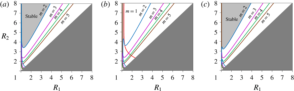
In figure 3, the instability regions on the
 $(R_{1},R_{2})$
-plane are plotted for
 $\unicode[STIX]{x1D6FD}=0$
and
 $\unicode[STIX]{x1D6FD}=-0.01$
. The lines of critical stability (the edges of the regions where
 $\text{Im}(\unicode[STIX]{x1D714})=0$
) of the modes
 $m=1$
, 2, 3, 4 and 5 are plotted in the physically meaningful domain
 $1<R_{1}<R_{2}$
, and the region in which all modes are stable is light-grey shaded. The case of
 $\unicode[STIX]{x1D6FD}=0$
was studied by Kizner et al. (Reference Kizner, Makarov, Kamp and van Heijst2013), and is shown here (figure 3
a) as a reference to see the changes made by the beta effect. Clearly, at
 $\unicode[STIX]{x1D6FD}=0$
the result is independent of the sign of
 $\unicode[STIX]{x1D6E4}_{1}$
, i.e. on the flow direction. But at
 $\unicode[STIX]{x1D6FD}=-0.01$
, a noticeable change is seen: while for
 $\unicode[STIX]{x1D6E4}_{1}=+1$
mode 2 broadens its stability region, for
 $\unicode[STIX]{x1D6E4}_{1}=-1$
, mode 2 becomes less stable, and, moreover, mode 1 develops instability as well on a vast part of the plane (figure 3
b,c). In the next subsection, this asymmetry between the two directions of the basic flow is elucidated.
5.2 Symmetry breaking for modes
$m\geqslant 2$

Stability and instability regions on the
 $(R_{1},R_{2})$
-plane for (a)
 $\unicode[STIX]{x1D6E4}_{1}=\pm 1,\unicode[STIX]{x1D6FD}=0$
, (b)
 $\unicode[STIX]{x1D6E4}_{1}=-1,\unicode[STIX]{x1D6FD}=-0.01$
and (c)
 $\unicode[STIX]{x1D6E4}_{1}=1,\unicode[STIX]{x1D6FD}=-0.01$
. Dark grey tone marks the physically irrelevant area; light grey, the stability region; curved lines (given in colour online) mark the boundaries of the instability regions (white area) of modes 1 to 5, and mode numbers appear next to these lines.

At sufficiently small
 $|\unicode[STIX]{x1D6FD}|$
and
 $\unicode[STIX]{x1D714}\neq 0$
, the expression
 $\unicode[STIX]{x1D6FD}r/\unicode[STIX]{x1D714}$
appearing in the argument of the modified Bessel function
 $\text{K}_{2m}$
in (4.8), is much smaller in absolute value than 1. We therefore may use the Laurent-series expansion of this function around zero for the case
 $m\geqslant 2$
, keeping, besides the multiplier, the terms up to the second power in
 $\unicode[STIX]{x1D6FD}r/\unicode[STIX]{x1D714}$
:
 $$\begin{eqnarray}\text{K}_{2m}\left(2\sqrt{-\frac{\unicode[STIX]{x1D6FD}r}{\unicode[STIX]{x1D714}}}\right)\approx \frac{1}{2}\left(-\frac{\unicode[STIX]{x1D714}}{\unicode[STIX]{x1D6FD}r}\right)^{m}\left((2m-1)!+(2m-2)!\left(\frac{\unicode[STIX]{x1D6FD}r}{\unicode[STIX]{x1D714}}\right)+\frac{(2m-3)!}{2}\left(\frac{\unicode[STIX]{x1D6FD}r}{\unicode[STIX]{x1D714}}\right)^{2}\right)\end{eqnarray}$$
(Abramowitz & Stegun Reference Abramowitz and Stegun1964). Equation (5.1) provides, in fact, the small-beta correction to the outer-region zero-
 $\unicode[STIX]{x1D6FD}$
streamfunction, which is proportional to
 $r^{-m}$
. Therefore, to the first order in
 $\unicode[STIX]{x1D6FD}$
, the coefficients of the eigenvalue equation (4.14) defined in appendix A (after dividing the equation by a constant to make
 $A=1$
) become
 $$\begin{eqnarray}A(\unicode[STIX]{x1D714})=1,\quad B(\unicode[STIX]{x1D714})=B_{0}\unicode[STIX]{x1D6E4}_{1}+B_{1}\unicode[STIX]{x1D6FD},\quad C(\unicode[STIX]{x1D714})=C_{0}\unicode[STIX]{x1D6E4}_{1}^{2}+C_{1}\unicode[STIX]{x1D6E4}_{1}\unicode[STIX]{x1D6FD},\end{eqnarray}$$
where the coefficients
 $B_{0},B_{1},C_{0}$
and
 $C_{1}$
are independent of
 $\unicode[STIX]{x1D6FD}$
,
 $\unicode[STIX]{x1D6E4}_{1}$
and
 $\unicode[STIX]{x1D714}$
, and are rational polynomials in
 $R,R_{1},R_{2}$
. The expressions for these coefficients for
 $m=2$
and 3 are given in appendix B. Since
 $\unicode[STIX]{x1D6E4}_{1}=\pm 1$
we substitute
 $\unicode[STIX]{x1D6E4}_{1}^{2}=1$
in (5.2), and get the quadratic equation in
 $\unicode[STIX]{x1D714}$
,
 $$\begin{eqnarray}\unicode[STIX]{x1D714}^{2}+(B_{0}\unicode[STIX]{x1D6E4}_{1}+B_{1}\unicode[STIX]{x1D6FD})\unicode[STIX]{x1D714}+(C_{0}+C_{1}\unicode[STIX]{x1D6E4}_{1}\unicode[STIX]{x1D6FD})=0,\end{eqnarray}$$
which is the first-order correction in
 $\unicode[STIX]{x1D6FD}$
to the quadratic equation obtained by Kizner et al. (Reference Kizner, Makarov, Kamp and van Heijst2013) in the case of
 $\unicode[STIX]{x1D6FD}=0$
; the zero-subscripted coefficients are equal to the ones found there.
As noted in § 4, the condition for instability is the existence of a non-real root to (5.3), which means that the discriminant
 $\unicode[STIX]{x1D6E5}$
of the quadratic equation is negative. This discriminant can be written as
 $$\begin{eqnarray}\unicode[STIX]{x1D6E5}=\unicode[STIX]{x1D6E5}_{0}+\unicode[STIX]{x1D6FD}\unicode[STIX]{x1D6E4}_{1}\unicode[STIX]{x1D6E5}_{1},\end{eqnarray}$$
where
 $$\begin{eqnarray}\unicode[STIX]{x1D6E5}_{0}=B_{0}^{2}-4C_{0}\end{eqnarray}$$
and
 $$\begin{eqnarray}\unicode[STIX]{x1D6E5}_{1}=2B_{0}B_{1}-4C_{1}\end{eqnarray}$$
are, respectively, the zero-
 $\unicode[STIX]{x1D6FD}$
discriminant of the equation, and its first correction term, which is coupled with
 $\unicode[STIX]{x1D6FD}\unicode[STIX]{x1D6E4}_{1}$
. The equation
 $\unicode[STIX]{x1D6E5}_{0}=0$
determines the stability bound in the
 $(R_{1},R_{2})$
-plane for the flat-bottom case. It is directly verified, that, on this bound,
 $\unicode[STIX]{x1D6E5}_{1}<0$
, hence
 $\unicode[STIX]{x1D6E5}>0$
(
 $\unicode[STIX]{x1D6E5}<0$
) at
 $\unicode[STIX]{x1D6FD}\unicode[STIX]{x1D6E4}_{1}<0$
(
 $\unicode[STIX]{x1D6FD}\unicode[STIX]{x1D6E4}_{1}>0$
). Thus, the region of stability
 $\unicode[STIX]{x1D6E5}\geqslant 0$
expands relative to the flat-bottom case if
 $\unicode[STIX]{x1D6E4}_{1}=1$
. When
 $\unicode[STIX]{x1D6E4}_{1}=-1$
, the beta effect is in an opposite trend destabilizing the flow. This can be seen from the comparison of figures 3(a) and 3(b), particularly for mode 2. For modes
 $m\geqslant 3$
the beta effect at
 $\unicode[STIX]{x1D6FD}=-0.01$
has a minor impact, which cannot be seen by the naked eye.
5.3 Onset of the mode-1 instability
The instability regions of mode 1 for
 $\unicode[STIX]{x1D6E4}_{1}=-1$
, for
 $\unicode[STIX]{x1D6FD}=10^{-5}$
,
 $\unicode[STIX]{x1D6FD}=10^{-4}$
and
 $\unicode[STIX]{x1D6FD}=10^{-3}$
. For each of these values of
 $\unicode[STIX]{x1D6FD}$
, the instability region is located on the right of the curved line labelled by this beta.

As can be seen from the comparison of figures 3(a) and 3(b), a dramatic change in the stability diagram occurs to mode 1. While at
 $\unicode[STIX]{x1D6FD}=0$
, mode 1 is entirely stable, even a small beta makes this mode unstable in a large region of the
 $(R_{1},R_{2})$
-plane.
To understand why this happens, we review the calculations done above in the presence of small
 $\unicode[STIX]{x1D6FD}$
, this time for mode
 $m=1$
. The first-order approximation of the modified Bessel function
 $\text{K}_{2}$
(appearing in (4.8)) at small
 $\unicode[STIX]{x1D6FD}$
is
 $$\begin{eqnarray}\text{K}_{2}\left(2\sqrt{-\frac{\unicode[STIX]{x1D6FD}r}{\unicode[STIX]{x1D714}}}\right)\approx -\frac{1}{2}\left(\frac{\unicode[STIX]{x1D714}}{\unicode[STIX]{x1D6FD}r}\right)\left(1+\frac{\unicode[STIX]{x1D6FD}r}{\unicode[STIX]{x1D714}}-\frac{1}{4}\left(2\ln \left(-\frac{\unicode[STIX]{x1D6FD}r}{\unicode[STIX]{x1D714}}\right)+4\unicode[STIX]{x1D6FE}-3\right)\left(\frac{\unicode[STIX]{x1D6FD}r}{\unicode[STIX]{x1D714}}\right)^{2}\right)\end{eqnarray}$$
(Abramowitz & Stegun Reference Abramowitz and Stegun1964). Equation (5.2) remains valid in this case, with the coefficients
 $B_{0},B_{1},C_{0}$
and
 $C_{1}$
for
 $m=1$
being given in appendix B; in particular,
 $C_{0}$
is zero. Substitution of (5.2) into (4.14) results in a quadratic equation,
 $$\begin{eqnarray}\unicode[STIX]{x1D714}^{2}+(B_{0}\unicode[STIX]{x1D6E4}_{1}+B_{1}\unicode[STIX]{x1D6FD})\unicode[STIX]{x1D714}+C_{1}\unicode[STIX]{x1D6E4}_{1}\unicode[STIX]{x1D6FD}=0.\end{eqnarray}$$
The condition for the existence of non-real roots,
 $\unicode[STIX]{x1D6E5}<0$
, is now
 $$\begin{eqnarray}\unicode[STIX]{x1D6E5}=\frac{R^{4}(R^{2}-R_{1}^{2})^{2}}{4R_{1}^{4}R_{2}^{4}}-P(R,R_{1},R_{2})\unicode[STIX]{x1D6E4}_{1}\unicode[STIX]{x1D6FD}<0,\end{eqnarray}$$
where
 $P(R,R_{1},R_{2})$
is a polynomial in
 $R$
,
 $R_{1}$
and
 $R_{2}$
, given in appendix B. Inequality (5.9) is never satisfied if
 $\unicode[STIX]{x1D6FD}=0$
, so in the case of
 $\unicode[STIX]{x1D6FD}=0$
, mode 1 is stable in the entire
 $(R_{1},R_{2})$
-plane, as shown formerly by Kizner et al. (Reference Kizner, Makarov, Kamp and van Heijst2013). Also, when
 $\unicode[STIX]{x1D6E4}_{1}=1$
, at sufficiently small
 $|\unicode[STIX]{x1D6FD}|$
, again, inequality (5.9) is not satisfied. However, for
 $\unicode[STIX]{x1D6E4}_{1}=-1$
, there is always a region in the
 $(R_{1},R_{2})$
-plane in which this inequality is satisfied and, therefore, instability takes place. The regions of the mode-1 instability on the
 $(R_{1},R_{2})$
-plane for the cases of
 $\unicode[STIX]{x1D6FD}=-10^{-5}$
,
 $-10^{-4}$
and
 $-10^{-3}$
are shown in figure 4. As
 $\unicode[STIX]{x1D6FD}$
gets larger in magnitude (but remains small enough to ensure the validity of approximation (5.7)), the instability regions expand, covering larger parts of the plane. Hence, in terms of the mode-1 instability too, the beta effect breaks the symmetry between the two alternative directions of the basic flow.
6 Stability diagrams and growth rates in the general case
Stability regions on the
 $(R_{1},R_{2})$
-plane for modes 1 to 5. (a)
 $\unicode[STIX]{x1D6E4}_{1}=1$
and
 $\unicode[STIX]{x1D6FD}=-0.1$
, (b)
 $\unicode[STIX]{x1D6E4}_{1}=-1$
and
 $\unicode[STIX]{x1D6FD}=-0.1$
, (c)
 $\unicode[STIX]{x1D6E4}_{1}=1$
and
 $\unicode[STIX]{x1D6FD}=-1$
, (d)
 $\unicode[STIX]{x1D6E4}_{1}=-1$
and
 $\unicode[STIX]{x1D6FD}=-1$
. Mode numbers (and colours online) as in figure 3.

Growth rates
 $m\text{Im}(\unicode[STIX]{x1D714})$
as functions of
 $R_{2}$
at
 $R_{1}=2.5$
, for (a)
 $\unicode[STIX]{x1D6E4}_{1}=1$
and
 $\unicode[STIX]{x1D6FD}=-0.1$
, (b)
 $\unicode[STIX]{x1D6E4}_{1}=-1$
and
 $\unicode[STIX]{x1D6FD}=-0.1$
, (c)
 $\unicode[STIX]{x1D6E4}_{1}=1$
and
 $\unicode[STIX]{x1D6FD}=-1$
, (d)
 $\unicode[STIX]{x1D6E4}_{1}=-1$
and
 $\unicode[STIX]{x1D6FD}=-1$
. Insets in the upper-right corners represent the growth rates in a unified scale. Mode numbers (and colours online) as in figure 3.

We proceed now to the general case of any negative
 $\unicode[STIX]{x1D6FD}$
(not necessarily
 $|\unicode[STIX]{x1D6FD}|\ll 1$
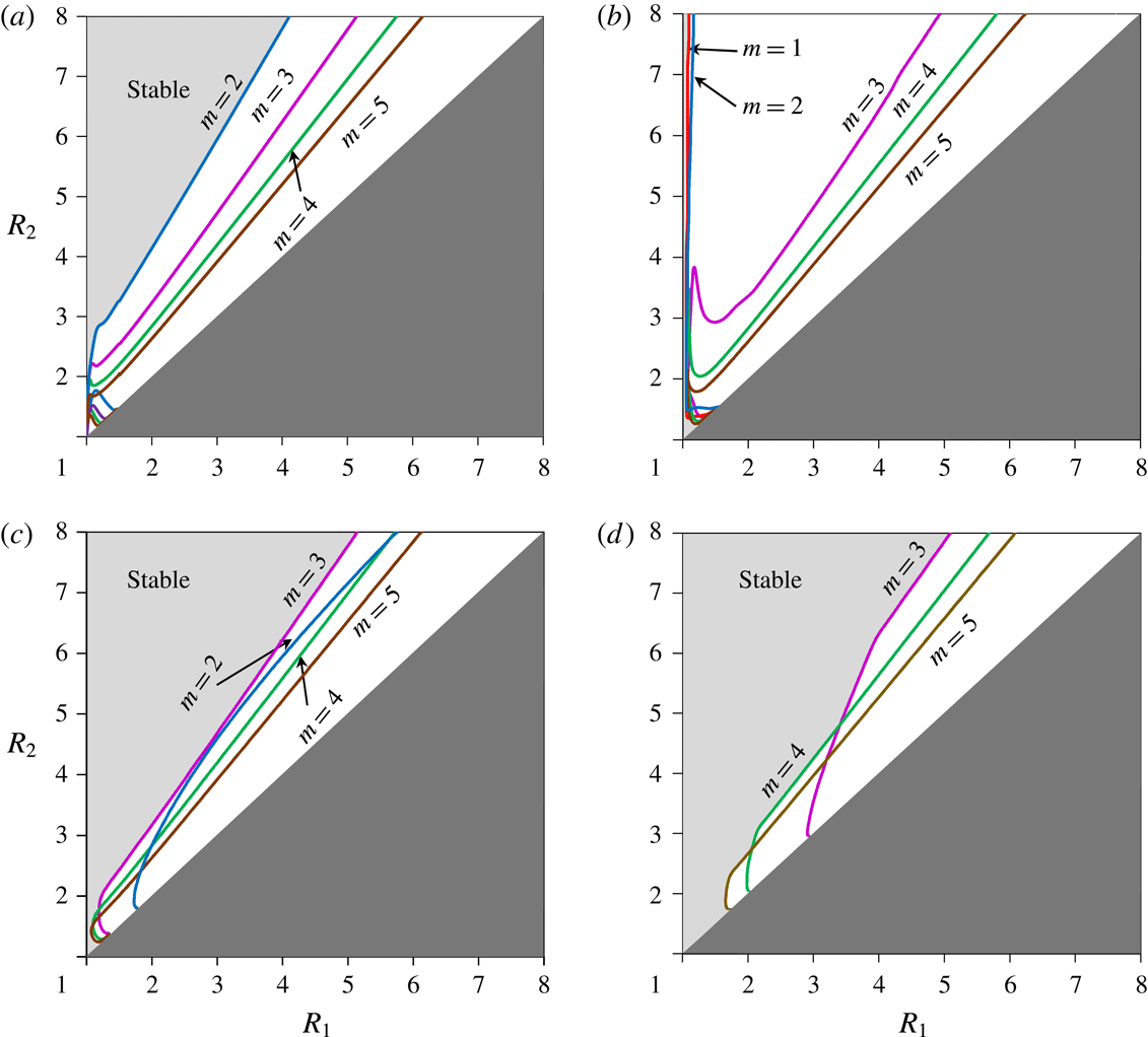
), in which the eigenvalue equation (4.14) is solved numerically. Figure 5 shows the stability regions for two specific values of beta,
 $\unicode[STIX]{x1D6FD}=-0.1$
and
 $\unicode[STIX]{x1D6FD}=-1$
, for the two alternatives,
 $\unicode[STIX]{x1D6E4}_{1}=+1$
and
 $\unicode[STIX]{x1D6E4}_{1}=-1$
.
In the case of
 $\unicode[STIX]{x1D6FD}=-0.1$
(figure 5
a,b), again a clear-cut distinction between the cases of
 $\unicode[STIX]{x1D6E4}_{1}=+1$
and
 $\unicode[STIX]{x1D6E4}_{1}=-1$
is seen. When
 $\unicode[STIX]{x1D6E4}_{1}=-1$
, the instability of mode 1 is observed in almost the entire
 $(R_{1},R_{2})$
-plane, excluding a thin strip very close to the line
 $R_{1}=R$
. The region of the mode-2 instability expands and becomes nearly as large as that of the mode-1 instability. Modes 3, 4 and 5 demonstrate little change in their instability regimes. On the other hand, at
 $\unicode[STIX]{x1D6E4}_{1}=+1$
the beta effect causes the stability regions to slightly enlarge in all modes.
The case of a strong beta effect is shown in figure 5(c,d). When
 $\unicode[STIX]{x1D6FD}=-1$
and
 $\unicode[STIX]{x1D6E4}_{1}=-1$
(figure 5
d), mode 1 is stable. The stabilization due to the beta effect is so strong that mode
 $m=2$
becomes stable in the entire
 $(R_{1},R_{2})$
-plane, and the first unstable mode is
 $m=3$
(figure 5
d). Also a significant shrinking of the instability regions is seen in the higher modes; the instability begins at higher values of
 $R_{1}$
compared to the low-beta regime. The fact that a clockwise flow is destabilized by weak slopes, while is stable at steeper slopes, is in accordance with the results by Poulin & Flierl (Reference Poulin and Flierl2005) mentioned in the Introduction. In fact, a clockwise flow is a prograde one, because it goes in the direction in which topographic Rossby waves propagate.
When
 $\unicode[STIX]{x1D6E4}_{1}=1$
(figure 5
c), mode 1 is still stable in the entire
 $(R_{1},R_{2})$
-plane, while mode 2 is more stable than mode 3. The fact that the bottom slope has a stabilizing effect on counterclockwise flows at all values of
 $\unicode[STIX]{x1D6FD}$
(compared to the flat-bottom case) is in accordance with the results by Li & McClimans (Reference Li and McClimans2000) and Poulin & Flierl (Reference Poulin and Flierl2005), who found that retrograde flow is always stabilized by the bottom topography. The curves of critical stability of modes 3, 4 and 5 are almost the same as in figure 5(a,b) (except the region where
 $R_{1}$
is close to 1). This is an indication that the dependence on
 $\unicode[STIX]{x1D6FD}$
is weak in these modes.
In figure 6, the growth rates of the first five modes are shown as functions of
 $R_{2}$
for the case of
 $R_{1}=2.5$
. The growth rates at
 $\unicode[STIX]{x1D6FD}=-0.1$
(figure 6
a,b) indicate, as discussed above, the difference between the counterclockwise and clockwise flows. The growth rates of modes
 $m\geqslant 2$
are, generally, slightly higher in the case of
 $\unicode[STIX]{x1D6E4}_{1}=1$
; yet the main difference is seen in mode 1. While at
 $\unicode[STIX]{x1D6E4}_{1}=-1$
, the mode-1 instability occurs in a large range of values of
 $R_{2}$
, it is totally absent in the case of
 $\unicode[STIX]{x1D6E4}_{1}=1$
. In figure 6(c,d) the growth rates are shown for
 $\unicode[STIX]{x1D6E4}_{1}=+1$
and
 $-1$
at
 $\unicode[STIX]{x1D6FD}=-1$
. When
 $\unicode[STIX]{x1D6E4}_{1}=+1$
the growth rates are higher relative to the flow with
 $\unicode[STIX]{x1D6FD}=-0.1$
, while at
 $\unicode[STIX]{x1D6E4}_{1}=-1$
, the growth rates are lower, and modes 2 and 3 exhibit no instability at all at this value of
 $R_{1}$
.
Stability regions for
 $\unicode[STIX]{x1D6E4}_{1}=-1$
,
 $\unicode[STIX]{x1D6FD}=-0.1$
, with stable regions due to monotonic PV profile marked. Mode numbers (and colours online) as in figure 3. Dashed lines indicate the boundaries of the regions, in which the sufficient stability condition (6.1) is fulfilled.

Parts of the stable regions shown in figure 5 can be intuitively understood in the following way. When the basic PV profile is monotonic (figure 2 c), it can be approximated with any degree of accuracy by a smooth monotonic profile having a negative PV gradient. Thus, according to the Rayleigh criterion (expressed in terms of PV), the flow should be stable. This argument suggests that the original non-smooth, stepwise profile should also be stable. The correctness of this intuitively achieved conclusion can be proved rigorously (appendix C).
So, a sufficient condition for the stability of a flow given by two uniform-PV rings is that the PV profile be a non-increasing function, i.e.
 $\unicode[STIX]{x1D6FD}R_{2}\leqslant \unicode[STIX]{x1D6E4}_{2}\leqslant \unicode[STIX]{x1D6E4}_{1}$
. With the use of (3.4), this can be written as
 $$\begin{eqnarray}\unicode[STIX]{x1D6FD}R_{2}\leqslant -\frac{\unicode[STIX]{x1D6E4}_{1}(R_{1}^{2}-R^{2})-\frac{2}{3}\unicode[STIX]{x1D6FD}(R_{2}^{3}-R^{3})}{R_{2}^{2}-R_{1}^{2}}\leqslant \unicode[STIX]{x1D6E4}_{1}.\end{eqnarray}$$
The sufficient stability condition (6.1) determines a region in the
 $(R_{1},R_{2})$
-plane which is part of the region of stability found by numerical solving of (4.14). This is seen in figure 7, which is a wider view of figure 5(b) for a larger range of values of
 $R_{1}$
and
 $R_{2}$
. The regions of instability of modes 1 to 5 are shown for the case of
 $\unicode[STIX]{x1D6FD}=-0.1$
and
 $\unicode[STIX]{x1D6E4}_{1}=-1$
. According to the definition of
 $\unicode[STIX]{x1D6E4}_{2}$
(see (3.4), which assures vanishing of the velocity outside the rings), the right of the inequalities (6.1) is satisfied when
 $R_{2}$
is larger than some critical value, which is independent of
 $R_{1}$
. For
 $\unicode[STIX]{x1D6FD}=-0.1$
this critical value is approximately
 $R_{2}=15.07$
. Above the line
 $R_{2}=15.07$
, the left of the inequalities (6.1) is the one that determines the region of guaranteed stability. Since the Rayleigh criterion is a sufficient condition for stability, there are regions where this condition is not satisfied, yet the flow is linearly stable. These are the light-grey zones marked ‘stable’. The above arguments allow us to assert that there is a chance for the development of instability in the flows with the PV profiles like in figure 2(a,b), but the flows with the PV profiles like in figure 2(c) are always stable.
7 Rossby-wave viewpoint on the transition to instability
Our aim in this section is to discuss in terms of Rossby waves the transition from stability to instability due to the beta effect. As an illustrative example we consider the case of the mode-1 stability/instability, which is of special importance for, in the flat-bottom case, this mode is always stable. When
 $\unicode[STIX]{x1D6FD}$
goes to zero, the eigenvalue equation (4.14) transforms into a quadratic equation, thus having two roots. This was shown in § 5 (see (5.3) and (5.8) valid for
 $m\geqslant 2$
and
 $m=1$
, respectively). In the general case of an arbitrary
 $\unicode[STIX]{x1D6FD}$
, equation (4.14) is transcendental, yet in all our high-resolution computations, only two eigenvalues were revealed for each
 $\unicode[STIX]{x1D6FD}$
. These correspond to two kinds of perturbations; one of them, whose eigenfrequency
 $\unicode[STIX]{x1D714}$
goes to zero as
 $\unicode[STIX]{x1D6FD}\rightarrow 0$
, will be termed the type-a perturbation, and the other one, the type-b perturbation. Starting from the flat-bottom case (
 $\unicode[STIX]{x1D6FD}=0$
), which can be fully treated analytically, we proceed to the case of
 $\unicode[STIX]{x1D6FD}<0$
, and follow the effect of increasing the magnitude of
 $\unicode[STIX]{x1D6FD}$
on the frequencies and patterns of each of the perturbation types. Our discussion below, which is of general nature, will be illustrated by examples with
 $R_{1}=2.5$
and
 $R_{2}=4$
(figures 8 and 9).
7.1 Flat-bottom case
Mode-1 perturbation frequencies. Roots of the eigenvalue equation (4.14) as functions of
 $\unicode[STIX]{x1D6FD}$
for
 $R_{1}=2.5$
and
 $R_{2}=4$
. (a)
 $\unicode[STIX]{x1D6E4}_{1}=-1$
, (b)
 $\unicode[STIX]{x1D6E4}_{1}=+1$
. Online, the real parts of the type-a and type-b frequencies are given by red and blue lines, respectively, and the imaginary parts by green lines.

Type-a (red online) and type-b (blue online) radial profiles of the mode-1 perturbation streamfunctions normalized to their peak values (taken at
 $r=R_{1}$
). Examples for
 $R_{1}=2.5$
and
 $R_{2}=4$
. (a)
 $\unicode[STIX]{x1D6FD}=0\;(\unicode[STIX]{x1D6E4}_{1}=\pm 1)$
, (b)
 $\unicode[STIX]{x1D6FD}=-0.1$
and
 $\unicode[STIX]{x1D6E4}_{1}=1$
and (c)
 $\unicode[STIX]{x1D6FD}=-0.001$
and
 $\unicode[STIX]{x1D6E4}_{1}=-1$
.

In the flat-bottom case, the background vorticity is absent, so the PV and relative vorticity are the same, i.e.
 $Q=\unicode[STIX]{x1D701}$
. As noted in § 4 (see also (5.8)), when
 $\unicode[STIX]{x1D6FD}=0$
, the eigenvalue equation is quadratic. Using the formulae for
 $C_{0}$
and
 $B_{0}$
provided in appendix B for the case of
 $m=1$
, we find from (5.8) the two solutions of this equation, i.e. the two eigenfrequencies:
 $$\begin{eqnarray}\unicode[STIX]{x1D714}_{a}=0,\quad \text{and}\quad \unicode[STIX]{x1D714}_{b}=\unicode[STIX]{x1D6E4}_{1}\frac{R^{2}(R_{1}^{2}-R^{2})}{2R_{1}^{2}R_{2}^{2}}.\end{eqnarray}$$
Here and below (§ 7.2), the subscripts
 $a$
and
 $b$
are used to distinguish between the two types of perturbation that, when taking the limit
 $\unicode[STIX]{x1D6FD}\rightarrow 0$
, have the frequencies given by formulae (7.1). Figure 8 shows the frequencies of the two types as functions of
 $\unicode[STIX]{x1D6FD}$
. In this section we consider the nature of the two types of perturbation in the flat-bottom case (
 $\unicode[STIX]{x1D6FD}=0$
), deferring the discussion of the beta effect to § 7.2.
Following the route outlined in the end of § 4 (for details, including the formulae for the coefficients of the couple of linear homogeneous equations in
 $d_{1}$
and
 $d_{2}$
, see Kizner et al.
Reference Kizner, Makarov, Kamp and van Heijst2013) and using (7.1), one obtains the ratios between the amplitudes of the deformations of the contours bounding the vorticity rings in each of the cases a and b:
 $$\begin{eqnarray}\left(\frac{d_{2}}{d_{1}}\right)_{a}=1,\quad \left(\frac{d_{2}}{d_{1}}\right)_{b}=\frac{R_{1}^{2}(R_{2}^{2}-R^{2})}{R_{2}^{2}(R_{1}^{2}-R^{2})}.\end{eqnarray}$$
According to (7.2), the type-a perturbation consists in equal deformation of the liquid boundaries, while in the case of the type-b perturbation, the deformations are unequal. The centre of the ‘vorticity mass’ of each of the deformed rings is defined as
 $\iint rQ\boldsymbol{r}\,\text{d}r\,\text{d}\unicode[STIX]{x1D703}/\iint rQ\,\text{d}r\,\text{d}\unicode[STIX]{x1D703}$
, where the integration is made over the areas occupied by either positive or negative vorticity, and the singular vorticity (4.15) is taken into account along with the uniform regular vorticity in the rings. Direct calculation shows that equal deformation of the contours (type-a perturbation) shifts the centres of mass relative to each other, whereas unequal deformation (type-b) keeps the centres of mass coincident. This result, which might look paradoxical at a first glance, is a consequence of the presence of a motionless island, that is, of the fact that the internal boundary of the inner ring remains unperturbed.
The discontinuities of the basic vorticity profile at the circles
 $r=R_{1}$
and
 $r=R_{2}$
give rise to the existence of the Rossby waves traveling in these circles, these waves being just the perturbations. Therefore, we could bypass formulae (7.1) and find the frequency
 $\unicode[STIX]{x1D714}$
of the perturbation as the phase velocity
 $\unicode[STIX]{x1D714}_{Ro}$
of the wave that runs at a discontinuity contour of the basic PV profile in the presence of a background (basic) flow. Clearly, the wave at the inner contour propagates in the same direction and at the same phase velocity as the wave at the outer contour, because the two waves must be synchronous. This phase velocity can be calculated by integrating the Rayleigh equation (4.5) in the neighbourhood of any of the singularities with the use of (3.2) and (4.15):
 $$\begin{eqnarray}\unicode[STIX]{x1D714}=\unicode[STIX]{x1D714}_{Ro}|_{R_{1,2}}=\frac{\bar{V}(R_{1,2})}{R_{1,2}}+\frac{\unicode[STIX]{x1D6F7}(R_{1,2})}{R_{1,2}d_{1,2}},\end{eqnarray}$$
where
 $R_{1,2}$
may be either
 $R_{1}$
or
 $R_{2}$
, and
 $d_{1,2}$
is either
 $d_{1}$
or
 $d_{2}$
. Using (2.1), (2.3), (4.4) and (4.5), in the case of
 $\unicode[STIX]{x1D714}=\unicode[STIX]{x1D714}_{a}=0$
(type-a perturbation with
 $d_{1}=d_{2}=d$
), the following equation relating the perturbation streamfunction and the basic velocity profile can be obtained:
 $$\begin{eqnarray}\frac{\bar{V}}{r}\left(\unicode[STIX]{x1D6F7}^{\prime \prime }+\frac{\unicode[STIX]{x1D6F7}^{\prime }}{r}-\frac{\unicode[STIX]{x1D6F7}}{r^{2}}\right)-\frac{\unicode[STIX]{x1D6F7}}{r}\left(\bar{V}^{\prime \prime }+\frac{\bar{V}^{\prime }}{r}-\frac{V}{r^{2}}\right)=0.\end{eqnarray}$$
Equation (7.4) may be rewritten, after multiplication by
 $r^{2}$
, as
 $$\begin{eqnarray}(r\unicode[STIX]{x1D6F7}^{\prime }\bar{V}-r\unicode[STIX]{x1D6F7}\bar{V}^{\prime })^{\prime }=0.\end{eqnarray}$$
Integration of (7.5) yields
 $$\begin{eqnarray}\unicode[STIX]{x1D6F7}^{\prime }\bar{V}-\unicode[STIX]{x1D6F7}\bar{V}^{\prime }=\frac{C}{r},\end{eqnarray}$$
for some constant
 $C$
. Since at
 $r>R_{2}$
the basic velocity
 $\bar{V}$
vanishes, we get from (7.6) that
 $C=0$
. Therefore, equation (7.6) yields
 $$\begin{eqnarray}\unicode[STIX]{x1D6F7}^{\prime }\bar{V}-\unicode[STIX]{x1D6F7}\bar{V}^{\prime }=\bar{V}^{2}\left(\frac{\unicode[STIX]{x1D6F7}}{\bar{V}}\right)^{\prime }=0.\end{eqnarray}$$
Equation (7.7) means that
 $\unicode[STIX]{x1D6F7}(r)$
is proportional to
 $\bar{V}(r)$
. According to (7.3), the proportionality coefficient is
 $-d$
; i.e.
 $\unicode[STIX]{x1D6F7}(r)=-d\bar{V}(r)$
. This profile normalized to the peak value taken at
 $r=R_{1}$
is shown in figure 9(a) (red online). Because the basic-flow velocity vanishes at
 $r\geqslant R_{2}$
, there is no wave at the outer contour, and therefore outside of it too. At the inner contour, however, the Rossby wave does exist and is a standing wave. In the case of the type-b perturbation, from (7.3) we get
 $\unicode[STIX]{x1D6F7}(R_{2})=-d_{2}(\bar{V}(R_{2})-\unicode[STIX]{x1D714}_{b}R_{2})=d_{2}\unicode[STIX]{x1D714}_{b}R_{2}\neq 0$
, therefore, there is a wave at the outer contour. There is also a wave in the exterior region, which is forced by the condition of continuity of
 $\unicode[STIX]{x1D6F7}$
at
 $r=R_{2}$
(4.9). The profile of
 $\unicode[STIX]{x1D6F7}$
corresponding to the type-b perturbation is shown in figure 9(a) (blue online). The basic flow is zero at
 $r\geqslant R_{2}$
, so by (7.3) the Rossby wave at the outer contour must run in the direction determined by the sign of the basic PV gradient. This singular gradient is positive if
 $\unicode[STIX]{x1D6E4}_{1}=+1$
and negative if
 $\unicode[STIX]{x1D6E4}_{1}=-1$
(figure 2). In other words, in the absence of a background flow, the frequency of the type-b perturbation,
 $\unicode[STIX]{x1D714}_{b}$
, has the sign of
 $\unicode[STIX]{x1D6E4}_{1}$
(see (7.1) and figure 8). Although the inner wave travels in a contour where the basic-PV gradient is opposite in sign to the basic-PV gradient at the outer contour, the background flow drags the wave in the counterclockwise direction when
 $\unicode[STIX]{x1D6E4}_{1}=+1$
, and in the clockwise direction when
 $\unicode[STIX]{x1D6E4}_{1}=-1$
, by this equalizing the phase velocities of the waves at the two contours.
It might be instructive to compare the behaviour of mode 1 in the presence of an island with that in a two-contour vortex (the case of no island). Our results regarding modes
 $m>1$
at
 $\unicode[STIX]{x1D6FD}=0$
can be transposed to the case of a two-contour vortex by just taking the limit
 $R\rightarrow 0$
. However, mode 1 requires a more delicate handling. This is because, at
 $R=0$
, both frequencies in (7.1) become zero. In such a situation, the matrix in (4.12) is defective, and the linear stability scheme presented in § 4 is incomplete. Stern (Reference Stern1987) considered this case (see also Flierl Reference Flierl1988; Stern & Radko Reference Stern and Radko1998) and showed that one of the two zero eigenfrequencies corresponds to equal deformations of the contours. Unlike the flow around an island, in a two-contour vortex, equal deformation of the contours, while keeping coincident the centres of the positive- and negative-vorticity masses, entails shifting of the vortex as a whole (in the linear approximation sense); this cannot cause unstable behaviour. The other zero eigenfrequency corresponds to unequal deformations of the contours, hence to a shift of the centres of positive- and negative-vorticity masses relative to each other, and to the emergence of a ‘dipole moment’ which initiates translation of the vortex. In the absolute frame of reference, translation represents unstable behaviour, though the instability develops linearly in time rather than exponentially. When treating this case, Stern considered a perturbation that deforms the inner contour only, but keeps the outer contour intact. A more formal treatment may be conducted if we write the perturbations in the form
 $\{q(r,\unicode[STIX]{x1D703},t),\unicode[STIX]{x1D713}(r,\unicode[STIX]{x1D703},t)\}=\{{\mathcal{Q}}(r,t),\unicode[STIX]{x1D6F7}(r,t)\}\text{e}^{\text{i}\unicode[STIX]{x1D703}}$
, with
 ${\mathcal{Q}}$
and
 $\unicode[STIX]{x1D6F7}$
being complex, instead of (4.3); the result, nonetheless, remains the same. In the presence of an island, the shift of the centres of positive and negative-vorticity masses (the type-a perturbation) does not cause unstable behaviour, as we saw above. Translation does not occur in this case because the island reflects the dipole moment; this effect can be explained with the use of the method of images for vortices near a circular wall (see e.g. Saffman Reference Saffman1979).
7.2 Conical topography
In figure 8, the computed mode-1 frequencies are shown for the type-a and type-b perturbations at
 $R_{1}=2.5$
and
 $R_{2}=4$
. In the presence of conical topography, there is a fundamental difference in the stability properties of the counterclockwise (
 $\unicode[STIX]{x1D6E4}_{1}=+1$
) and clockwise (
 $\unicode[STIX]{x1D6E4}_{1}=-1$
) flows. Namely, mode 1 is always stable in the first case (
 $\unicode[STIX]{x1D714}$
is real at any
 $\unicode[STIX]{x1D6FD}$
), but may be unstable in the second case (§§ 5 and 6); the instability of a clockwise flow occurs when
 $\unicode[STIX]{x1D6FD}$
is smaller than some critical value labelled
 $\unicode[STIX]{x1D6FD}_{Cr}$
in figure 8. Another observation is that always
 $\text{Re}(\unicode[STIX]{x1D714}_{a})<0$
at
 $\unicode[STIX]{x1D6FD}\neq 0$
; therefore, the type-a perturbation runs in the clockwise direction independently of the sign of
 $\unicode[STIX]{x1D6E4}_{1}$
. The type-b perturbation runs counterclockwise when
 $\unicode[STIX]{x1D6E4}_{1}=+1$
, and clockwise when
 $\unicode[STIX]{x1D6E4}_{1}=-1$
.
The perturbation of type-b in the flat-bottom case has a non-zero phase velocity, as explained above. According to (3.2) and (3.4), in the presence of a weak slope, the PV jump at
 $R_{1}$
is
 $$\begin{eqnarray}\unicode[STIX]{x1D6E4}_{2}-\unicode[STIX]{x1D6E4}_{1}=-\frac{R_{2}^{2}-R^{2}}{R_{2}^{2}-R_{1}^{2}}\unicode[STIX]{x1D6E4}_{1}+\frac{2}{3}\frac{R_{2}^{3}-R^{3}}{R_{2}^{2}-R_{1}^{2}}\unicode[STIX]{x1D6FD},\end{eqnarray}$$
and the PV jump at
 $R_{2}$
is
 $$\begin{eqnarray}\unicode[STIX]{x1D6FD}R_{2}-\unicode[STIX]{x1D6E4}_{2}=\frac{R_{1}^{2}-R^{2}}{R_{2}^{2}-R_{1}^{2}}\unicode[STIX]{x1D6E4}_{1}-\frac{1}{3}\frac{3R_{1}^{2}R_{2}-R_{2}^{3}-2R^{3}}{R_{2}^{2}-R_{1}^{2}}\unicode[STIX]{x1D6FD}.\end{eqnarray}$$
Counterclockwise flows are those with
 $\unicode[STIX]{x1D6E4}_{1}=1$
. Therefore as
 $\unicode[STIX]{x1D6FD}$
decreases, that is
 $|\unicode[STIX]{x1D6FD}|$
increases, the PV jump at
 $R_{1}$
increases in magnitude; the influence of
 $\unicode[STIX]{x1D6FD}$
on the PV jump at
 $R_{2}$
(7.8) depends on the sign of the expression
 $3R_{1}^{2}R_{2}-R_{2}^{3}-2R^{3}$
. If
 $3R_{1}^{2}R_{2}-R_{2}^{3}-2R^{3}$
is positive (negative), the jump at
 $R_{2}$
increases (decreases) in magnitude as the magnitude of
 $\unicode[STIX]{x1D6FD}$
increases. For the case of
 $R_{1}=2.5$
and
 $R_{2}=4$
chosen to illustrate our discussion, we get
 $3R_{1}^{2}R_{2}-R_{2}^{3}-2R^{3}=9>0$
. Thus, the PV jump across each of the contours increases with increasing
 $|\unicode[STIX]{x1D6FD}|$
. This causes the wave (which exists due to the gradient of the basic PV) to propagate faster (figure 8
a). In clockwise flows,
 $\unicode[STIX]{x1D6E4}_{1}=-1$
. Therefore, as
 $\unicode[STIX]{x1D6FD}$
(which is negative) grows in magnitude, the magnitude of the PV jump at
 $R_{1}$
decreases. Again, the influence of
 $\unicode[STIX]{x1D6FD}$
on the PV jump at
 $R_{2}$
(7.9) depends on the sign of the expression
 $3R_{1}^{2}R_{2}-R_{2}^{3}-2R^{3}$
. If
 $3R_{1}^{2}R_{2}-R_{2}^{3}-2R^{3}$
is positive (negative), the jump at
 $R_{2}$
decreases (increases) in magnitude as
 $|\unicode[STIX]{x1D6FD}|$
increases. Thus for the case of
 $R_{1}=2.5$
and
 $R_{2}=4$
, the phase velocity of the wave gets smaller when
 $|\unicode[STIX]{x1D6FD}|$
increases (figure 8
b). So, in this example, the beta effect on the PV jumps is opposite in clockwise and counterclockwise flows.
Let
 $\text{Im}(\unicode[STIX]{x1D714})=0$
, so we may write
 $\unicode[STIX]{x1D714}$
instead of
 $\text{Re}(\unicode[STIX]{x1D714})$
. This condition holds at any
 $\unicode[STIX]{x1D6FD}$
if
 $\unicode[STIX]{x1D6E4}_{1}=+1$
(figure 8
a) and at
 $\unicode[STIX]{x1D6FD}_{Cr}\leqslant \unicode[STIX]{x1D6FD}\leqslant 0$
if
 $\unicode[STIX]{x1D6E4}_{1}=-1$
(figure 8
b). As (4.8) stands for, the perturbation streamfunction outside the uniform-PV rings is proportional to the modified Bessel function
 $\text{K}_{2}(2\sqrt{-\unicode[STIX]{x1D6FD}r/\unicode[STIX]{x1D714}})$
when
 $\unicode[STIX]{x1D6FD}\neq 0$
. Thus, the sign of
 $\unicode[STIX]{x1D714}$
determines the spatial pattern of the perturbation in the outer region. At positive
 $\unicode[STIX]{x1D714}$
this function is monotonic and drops exponentially to zero at infinity. Therefore, the corresponding perturbation may be categorized as an edge wave. This is the case of the type-b perturbation at
 $\unicode[STIX]{x1D6E4}_{1}=+1$
, whose profiles are shown in figure 9(a,b) (blue online). At negative
 $\unicode[STIX]{x1D714}$
, the argument in
 $\text{K}_{2}$
is imaginary, so this function alternates and drops as
 $r^{-1/4}$
when
 $r\rightarrow \infty$
. This is the case of the type-a perturbation at
 $\unicode[STIX]{x1D6E4}_{1}=+1$
and of the two types of perturbation at
 $\unicode[STIX]{x1D6E4}_{1}=-1$
with
 $\unicode[STIX]{x1D6FD}_{Cr}<\unicode[STIX]{x1D6FD}<0$
(figure 8
b). The corresponding perturbation has the potentiality to radiate energy to infinity; therefore we may categorize it as a radiating wave (profile ‘a’ in figure 9
b and profiles ‘a’ and ‘b’ in figure 9
c). However, draining of energy does not occur at
 $\unicode[STIX]{x1D6E4}_{1}=+1$
and also at
 $\unicode[STIX]{x1D6E4}_{1}=-1$
as long as
 $\unicode[STIX]{x1D6FD}$
is small enough in magnitude because under these conditions mode 1 is stable, i.e. an infinitesimally small perturbation remains small. At
 $\unicode[STIX]{x1D6E4}_{1}=-1$
, as
 $\unicode[STIX]{x1D6FD}$
crosses (from right to left) the bifurcation level
 $\unicode[STIX]{x1D6FD}=\unicode[STIX]{x1D6FD}_{Cr}$
, the frequency
 $\unicode[STIX]{x1D714}$
, and hence the argument of the function
 $\text{K}_{2}$
, get complex (i.e. instability arises). The perturbation in the outer region, while remaining alternating, becomes now growing in time. The spatial decay of the perturbation becomes exponential, but in the vicinity of the crossover point, the rate of this decay is small. In such circumstances, a growing wave does not radiate energy to infinity, but nevertheless, the energy can be drained to regions distant from the uniform-PV rings, so at
 $\unicode[STIX]{x1D6FD}<\unicode[STIX]{x1D6FD}_{Cr}$
we get radiating instability (cf. Talley Reference Talley1983; Kamenkovich & Pedlosky Reference Kamenkovich and Pedlosky1996).
The bifurcation to instability occurs when the frequencies of the perturbations of types a and b have opposite trends as functions of
 $\unicode[STIX]{x1D6FD}$
, that is, their real parts approach each other. When
 $\unicode[STIX]{x1D6E4}_{1}=-1$
, the type-a and type-b perturbations converge both in phase velocity and in shape. This makes possible the interaction between the two types of perturbations. In fact, as they arrive at the same phase velocity at the bifurcation point, the waves of the two types phase-lock and enhance each other, causing the emergence of instability. When
 $\unicode[STIX]{x1D6E4}_{1}=+1$
, the type-a and type-b frequencies diverge with increasing
 $|\unicode[STIX]{x1D6FD}|$
, therefore instability cannot take place.
We note that the instabilities of mode
 $m\geqslant 2$
can be explained in the same manner. For
 $m\geqslant 2$
, in the flat-bottom case, the perturbations of the two types propagate with non-zero phase velocities, having the sign of
 $\unicode[STIX]{x1D6E4}_{1}$
. When the topography is incorporated, the radiating Rossby wave outside the rings advances the type of perturbation with the smaller phase velocity in its direction; this may cause the phase velocities of the waves of the two types to equate, thus giving rise to instability.
8 Conclusion
We have determined, in an essentially analytical way, the stability/instability regions in the parameter space of a circular flow around an island with the sea bottom sloping offshore (
 $\unicode[STIX]{x1D6FD}<0$
). The flow is composed of two uniform-PV rings having outer radii
 $R_{1}$
and
 $R_{2}$
. The non-dimensional PV in the inner ring is
 $\unicode[STIX]{x1D6E4}_{1}=+1$
(counterclockwise flow near the island) or
 $\unicode[STIX]{x1D6E4}_{1}=-1$
(clockwise flow near the island), the constant PV in the outer ring being chosen so as to make the net circulation zero. The azimuthal normal-mode analysis has led to a transcendental eigenvalue equation for the frequency
 $\unicode[STIX]{x1D714}$
.
For small magnitudes of
 $\unicode[STIX]{x1D6FD}$
, the fundamental difference between the two alternative directions,
 $\unicode[STIX]{x1D6E4}_{1}=+1$
and
 $\unicode[STIX]{x1D6E4}_{1}=-1$
, was demonstrated through the comparison of the instability regions in the
 $(R_{1},R_{2})$
-plane. For a counterclockwise flow over a slightly sloping bottom, the stability region of mode 2 was shown to be a little bigger than in the flat-bottom case. For a clockwise flow, mode 1 was found to bifurcate to instability in a large part of the parameter plane. For mode 1, the first-order asymptotic analysis in
 $\unicode[STIX]{x1D6FD}$
of the eigenvalue equation revealed that only clockwise flows are sensitive in their stability/instability properties to the effect of weak slope (small beta).
Steeper slopes generally have a tendency to stabilize the flow, with a larger effect on the flows with
 $\unicode[STIX]{x1D6E4}_{1}=1$
. A flow, which is counterclockwise near the cylinder (
 $\unicode[STIX]{x1D6E4}_{1}=1$
), entirely stabilizes with respect to mode-2 perturbations when
 $\unicode[STIX]{x1D6FD}=-1$
. A flow with
 $\unicode[STIX]{x1D6E4}_{1}=-1$
exhibits higher stability than in the small-beta regime: mode 1 becomes stable in almost the whole parameter plane (for weak slopes it is almost entirely unstable), while mode 2 enlarges considerably its stability region.
The Rayleigh criterion was extended to the case of stepwise-PV profiles, and by this, part of the parameter plane
 $(R_{1},R_{2})$
was analytically shown to obey a sufficient stability condition. It was also shown that the stability regions found via Rayleigh criterion are not exhaustive, and additional domains of stability do exist in the parameter plane. This is in agreement with other known flow configurations (see e.g. Lin Reference Lin1944). A physical interpretation of the onset of instability is provided, based on the consideration of the Rossby waves that develop on the two PV discontinuity contours and outside of the PV rings.
The next step in our research will be a numerical investigation of the nonlinear stage of the development of instabilities in stepwise-PV flows around an island. Apart from the currents around islands, after some modification, the beta-cone concept can be applied to the treatment of flows in the presence of a conical beta effect in a planetary scale, namely, of the Antarctic circumpolar current. This issue will be considered separately elsewhere.
Acknowledgements
This research was supported by the US–Israel Science Foundation (BSF), grant no. 2014206. The contribution of M.R. to this article is part of his work towards the PhD degree.
Appendix A. Eigenvalue equation coefficients
Here the explicit expressions for the coefficients of the eigenvalue equation (4.14) are provided. We define
 $$\begin{eqnarray}\left.\begin{array}{@{}c@{}}m_{11}={\displaystyle \frac{2mR_{1}^{2m-1}(R_{2}^{2m}-R^{2m})}{(R^{2m}-R_{1}^{2m})(R_{2}^{2m}-R_{1}^{2m})}},\\ m_{12}={\displaystyle \frac{2m}{R_{1}^{1+m}R_{2}^{-m}-R_{1}^{1-m}R_{2}^{m}}},\\ m_{21}={\displaystyle \frac{2m}{R_{1}^{m}R_{2}^{1-m}-R_{1}^{-m}R_{2}^{1+m}}},\\ m_{22}={\displaystyle \frac{m(R_{1}^{2m}+R_{2}^{2m})}{R_{2}(R_{1}^{2m}-R_{2}^{2m})}}-{\displaystyle \frac{m}{R_{2}}}+\sqrt{-{\displaystyle \frac{\unicode[STIX]{x1D6FD}R_{2}}{\unicode[STIX]{x1D714}}}}{\displaystyle \frac{\text{K}_{2m+1}(2\sqrt{-\unicode[STIX]{x1D6FD}R_{2}/\unicode[STIX]{x1D714}})}{R_{2}\text{K}_{2m}(2\sqrt{-\unicode[STIX]{x1D6FD}R_{2}/\unicode[STIX]{x1D714}})}}.\end{array}\right\}\end{eqnarray}$$
With these definitions the elements of the matrix appearing in (4.12) are
 $$\begin{eqnarray}\left.\begin{array}{@{}c@{}}\unicode[STIX]{x1D614}_{11}=\left({\displaystyle \frac{\bar{V}(R_{1})}{R_{1}}}-\unicode[STIX]{x1D714}\right)m_{11}-{\displaystyle \frac{\unicode[STIX]{x1D6E4}_{2}-\unicode[STIX]{x1D6E4}_{1}}{R_{1}}},\quad \unicode[STIX]{x1D614}_{12}=-\left({\displaystyle \frac{\bar{V}(R_{1})}{R_{1}}}-\unicode[STIX]{x1D714}\right)m_{12},\\ \unicode[STIX]{x1D614}_{21}=\unicode[STIX]{x1D714}m_{21},\quad \unicode[STIX]{x1D614}_{22}=\unicode[STIX]{x1D714}m_{22}-{\displaystyle \frac{\unicode[STIX]{x1D6FD}R_{2}-\unicode[STIX]{x1D6E4}_{2}}{R_{2}}}.\end{array}\right\}\end{eqnarray}$$
Then the coefficients of (4.14) are
 $$\begin{eqnarray}\left.\begin{array}{@{}c@{}}A(\unicode[STIX]{x1D714})=-m_{12}m_{21}-m_{11}m_{22},\\ B(\unicode[STIX]{x1D714})=-{\displaystyle \frac{(\unicode[STIX]{x1D6FD}R_{2}-\unicode[STIX]{x1D6E4}_{2})m_{11}}{R_{2}}}-{\displaystyle \frac{(\unicode[STIX]{x1D6E4}_{2}-\unicode[STIX]{x1D6E4}_{1})m_{22}}{R_{1}}}+{\displaystyle \frac{\bar{V}(R_{1})}{R_{1}}}m_{12}m_{21}+{\displaystyle \frac{\bar{V}(R_{1})}{R_{1}}}m_{11}m_{22},\\ C(\unicode[STIX]{x1D714})={\displaystyle \frac{(\unicode[STIX]{x1D6FD}R_{2}-\unicode[STIX]{x1D6E4}_{2})(\unicode[STIX]{x1D6E4}_{2}-\unicode[STIX]{x1D6E4}_{1}+\bar{V}(R_{1})m_{11})}{R_{1}R_{2}}}.\end{array}\right\}\end{eqnarray}$$
Appendix B. First-order correction coefficients
The expressions for the coefficients appearing in (5.2) are provided below for
 $m=1$
, 2 and 3.
Mode 1:
 $$\begin{eqnarray}\displaystyle B_{0}=-\frac{R_{1}^{2}R^{2}-R^{4}}{2R_{1}^{2}R_{2}^{2}},\quad B_{1}=-\frac{R^{5}+R^{3}R_{2}^{2}-3R^{2}R_{1}^{2}R_{2}-R^{2}R_{2}^{3}-R_{1}^{3}R_{2}^{2}+3R_{1}^{2}R_{2}^{3}}{3R_{1}^{2}R_{2}^{2}}, & & \displaystyle\end{eqnarray}$$
 $$\begin{eqnarray}\displaystyle C_{0}=0,\quad C_{1}=-\frac{(R-R_{2})(R+R_{1})(R-R_{1})^{2}(RR_{1}+RR_{2}+R_{1}R_{2})}{6R_{2}^{2}R_{1}^{2}(R_{1}+R_{2})}. & & \displaystyle\end{eqnarray}$$
The polynomial
 $P(R,R_{1},R_{2})$
appearing in inequality (5.9) is:
 $$\begin{eqnarray}\displaystyle P(R,R_{1},R_{2}) & = & \displaystyle (R^{2}-R_{1}^{2})(\!R^{7}R_{1}+R^{7}R_{2}+R^{5}R_{1}R_{2}^{2}\nonumber\\ \displaystyle & & \displaystyle +\,R^{5}R_{2}^{3}-3R^{4}R_{1}^{3}R_{2}-3R^{4}R_{1}^{2}R_{2}^{2}-R^{4}R_{1}R_{2}^{3}-R^{4}R_{2}^{4}-2R^{3}R_{1}^{3}R_{2}^{2}\nonumber\\ \displaystyle & & \displaystyle -\,2R^{3}R_{1}^{2}R_{2}^{3}+R^{2}R_{1}^{4}R_{2}^{2}+4R^{2}R_{1}^{3}R_{2}^{3}+5R^{2}R_{1}^{2}R_{2}^{4}\nonumber\\ \displaystyle & & \displaystyle -\,2R_{1}^{4}R_{2}^{4} )\!/[3R_{1}^{4}R_{2}^{4}(R_{1}+R_{2})].\end{eqnarray}$$
Mode 2:
 $$\begin{eqnarray}B_{0}=-(R_{1}^{4}R_{2}^{4}-2R^{2}R_{1}^{2}R_{2}^{4}+R^{4}R_{1}^{4}+R^{4}R_{1}^{2}R_{2}^{2}+R^{4}R_{2}^{4}-R^{6}R_{1}^{2}-R^{6}R_{2}^{2})/(4R_{2}^{4}R_{1}^{4}),\end{eqnarray}$$
 $$\begin{eqnarray}\displaystyle B_{1} & = & \displaystyle -(\!R^{7}R_{1}^{2}+R^{7}R_{2}^{2}-2R^{4}R_{1}^{4}R_{2}-R^{4}R_{1}^{2}R_{2}^{3}-R^{4}R_{2}^{5}\nonumber\\ \displaystyle & & \displaystyle +\,2R^{3}R_{1}^{2}R_{2}^{4}-2R_{1}^{5}R_{2}^{4}+2R_{1}^{4}R_{2}^{5} )\!/(6R_{1}^{4}R_{2}^{4}),\end{eqnarray}$$
 $$\begin{eqnarray}C_{0}=(R^{2}-R_{2}^{2})(R^{2}-R_{1}^{2})^{3}/(16R_{2}^{4}R_{1}^{4}),\end{eqnarray}$$
 $$\begin{eqnarray}\displaystyle C_{1} & = & \displaystyle -(R-R_{2})(R+R_{1})(R-R_{1})^{2} (\!2R^{5}R_{1}+2R^{5}R_{2}+2R^{4}R_{1}^{2}+2R^{4}R_{1}R_{2}\nonumber\\ \displaystyle & & \displaystyle +\,2R^{4}R_{2}^{2}+R^{3}R_{1}^{3}+3R^{3}R_{1}^{2}R_{2}+3R^{3}R_{1}R_{2}^{2}+R^{3}R_{2}^{3}-R^{2}R_{1}^{4}-2R^{2}R_{1}^{3}R_{2}\nonumber\\ \displaystyle & & \displaystyle -\,2R^{2}R_{1}^{2}R_{2}^{2}+2R^{2}R_{1}R_{2}^{3}+R^{2}R_{2}^{4}-3RR_{1}^{4}R_{2}-4RR_{1}^{3}R_{2}^{2}+2RR_{1}R_{2}^{4}\nonumber\\ \displaystyle & & \displaystyle +\,RR_{2}^{5}-3R_{1}^{2}R_{2}^{2}-R_{1}^{3}R_{2}^{3}+R_{1}^{2}R_{2}^{4}+R_{1}R_{2}^{5} )\!/[24R_{1}^{4}R_{2}^{4}(R_{1}+R_{2})].\end{eqnarray}$$
Mode 3:
 $$\begin{eqnarray}B_{0}=(R^{2}-R_{1}^{2})(R^{6}R_{1}^{4}+R^{6}R_{1}^{2}R_{2}^{2}+R^{6}R_{2}^{4}-R^{4}R_{2}^{6}-R^{2}R_{1}^{2}R_{2}^{6}+2R_{1}^{4}R_{2}^{6})/(6R_{1}^{6}R_{2}^{6}),\end{eqnarray}$$
 $$\begin{eqnarray}\displaystyle B_{1} & = & \displaystyle -(\!5R^{9}R_{1}^{4}+5R^{9}R_{1}^{2}R_{2}^{2}+5R^{9}R_{2}^{4}-9R^{6}R_{1}^{6}R_{2}-5R^{6}R_{1}^{4}R_{2}^{3}-5R^{6}R_{1}^{2}R_{2}^{5}\nonumber\\ \displaystyle & & \displaystyle -\,5R^{6}R_{2}^{7}+15R^{3}R_{1}^{4}R_{2}^{6}-15R_{1}^{7}R_{2}^{6}+9R_{1}^{6}R_{2}^{7} )\!/(45R_{1}^{6}R_{2}^{6}),\end{eqnarray}$$
 $$\begin{eqnarray}C_{0}=(R^{2}-R_{2}^{2})(R^{2}-R_{1}^{2})^{3}(2R^{2}R_{1}^{2}+R^{2}R_{2}^{2}+R_{1}^{4}+2R_{1}2^{2}R_{2}^{2})/(36R_{1}^{6}R_{2}^{6}),\end{eqnarray}$$
 $$\begin{eqnarray}\displaystyle C_{1} & = & \displaystyle -(R-R_{2})(R+R_{1})(R-R_{1})^{2} (\!20R^{7}R_{1}^{3}+20R^{7}R_{1}^{2}R_{2}+10R^{7}R_{1}R_{2}^{2}\nonumber\\ \displaystyle & & \displaystyle +\,10R^{7}R_{2}^{3}+20R^{6}R_{1}^{4}+40R^{6}R_{1}^{3}R_{2}+30R^{6}R_{1}^{2}R_{2}^{2}+20R^{6}R_{1}R_{2}^{3}+10R^{6}R_{2}^{4}+15R^{5}R_{1}^{5}\nonumber\\ \displaystyle & & \displaystyle +\,35R^{5}R_{1}^{4}R_{2}+45R^{5}R_{1}^{3}R_{2}^{2}+35R^{5}R_{1}^{2}R_{2}^{3}+15R^{5}R_{1}R_{2}^{4}+5R^{5}R_{2}^{5}-3R^{4}R_{1}^{5}R_{2}\nonumber\\ \displaystyle & & \displaystyle +\,7R^{4}R_{1}^{4}R_{2}^{2}+39R^{4}R_{1}^{3}R_{2}^{3}+19R^{4}R_{1}^{2}R_{2}^{4}+9R^{4}R_{1}R_{2}^{5}+4R^{4}R_{2}^{6}-5R^{3}R_{1}^{7}-23R^{3}R_{1}^{6}R_{2}\nonumber\\ \displaystyle & & \displaystyle -\,36R^{3}R_{1}^{5}R_{2}^{2}-4R^{3}R_{1}^{4}R_{2}^{3}+18R^{3}R_{1}^{3}R_{2}^{4}+8R^{3}R_{1}^{2}R_{2}^{5}+8R^{3}R_{1}R_{2}^{6}+4R^{3}R_{2}^{7}-5R^{2}R_{1}^{8}\nonumber\\ \displaystyle & & \displaystyle -\,19R^{2}R_{1}^{7}R_{2}-47R^{2}R_{1}^{6}R_{2}^{2}-42R^{2}R_{1}^{5}R_{2}^{3}-20R^{2}R_{1}^{4}R_{2}^{4}+12R^{2}R_{1}^{3}R_{2}^{5}+12R^{2}R_{1}^{2}R_{2}^{6}\nonumber\\ \displaystyle & & \displaystyle +\,4R^{2}R_{1}R_{2}^{7}-14RR_{1}^{8}R_{2}-28RR_{1}^{7}R_{2}^{2}-38RR_{1}^{6}R_{2}^{3}-33RR_{1}^{5}R_{2}^{4}-RR_{1}^{4}R_{2}^{5}+16RR_{1}^{3}R_{2}^{6}\nonumber\\ \displaystyle & & \displaystyle +\,8RR_{1}^{2}R_{2}^{7}-14R_{1}^{8}R_{2}^{2}-14R_{1}^{7}R_{2}^{3}-24R_{1}^{6}R_{2}^{4}-9R_{1}^{5}R_{2}^{5}+8R_{1}^{4}R_{2}^{6}\nonumber\\ \displaystyle & & \displaystyle +\,8R_{1}^{3}R_{2}^{7} )\!/[270R_{1}^{6}R_{2}^{6}(R_{1}+R_{2})].\end{eqnarray}$$
Appendix C. General PV profiles: a sufficient stability condition
In § 6 a heuristic argument for the correctness of the Rayleigh necessary condition for instability of a radially symmetric flow with a stepwise PV profile was suggested. A rigorous proof that follows the main steps of the proof for a smooth flow (e.g. Pedlosky Reference Pedlosky2013a ; Vallis Reference Vallis2017) is provided below. Solodoch, Stewart & McWilliams (Reference Solodoch, Stewart and McWilliams2016), who considered annular two-layer circularly symmetric flows, derived this criterion for the weighted (over layers) mean PV profile, decomposing the perturbation into azimuthal normal modes. In the case of sloping bottom topography, this mean flow is an analogue to the barotropic flow component in the case of a flat-bottom two-layer model (cf. Kizner et al. Reference Kizner, Berson, Reznik and Sutyrin2003). Regarding barotropic flows, our derivation is more general, because it does not use the modal decomposition and takes into account the possibility for the existence of singularities in the PV gradient (that is, jumps in the PV profile). We also allow one of the boundaries to be infinity.
We depart from (4.2), which is a linearized version of (2.6), and introduce a new variable,
 $\unicode[STIX]{x1D702}$
, via the equation
 $$\begin{eqnarray}q=\unicode[STIX]{x1D702}\frac{\text{d}\bar{Q}}{\text{d}r}.\end{eqnarray}$$
While
 $\text{d}\bar{Q}/\text{d}r$
may have singularities,
 $\unicode[STIX]{x1D702}$
is a smooth function of the coordinates
 $r$
and
 $\unicode[STIX]{x1D703}$
; this is because the singularities of
 $\bar{Q}$
and
 $q$
(if any) occur at the same circles
 $r=R_{1}$
and
 $r=R_{2}$
, and are given by delta functions ((3.2) and (4.15), see also Kizner et al.
Reference Kizner, Makarov, Kamp and van Heijst2013). Substitution of (C 1) into (4.2) and multiplication by
 $\unicode[STIX]{x1D702}$
yields
 $$\begin{eqnarray}\frac{1}{2}\frac{\unicode[STIX]{x2202}\unicode[STIX]{x1D702}^{2}}{\unicode[STIX]{x2202}t}+\frac{\unicode[STIX]{x2202}}{\unicode[STIX]{x2202}\unicode[STIX]{x1D703}}\frac{\bar{V}\unicode[STIX]{x1D702}^{2}}{2r}=\frac{1}{r}\frac{\unicode[STIX]{x2202}\unicode[STIX]{x1D713}}{\unicode[STIX]{x2202}\unicode[STIX]{x1D703}}\unicode[STIX]{x1D702}.\end{eqnarray}$$
Multiplying (C 2) by
 $r^{2}\,\text{d}\bar{Q}/\text{d}r$
and integrating it with respect to
 $r$
and
 $\unicode[STIX]{x1D703}$
gives, with the use of (C 1),
 $$\begin{eqnarray}\frac{\unicode[STIX]{x2202}}{\unicode[STIX]{x2202}t}\int _{R}^{\infty }\int _{0}^{2\unicode[STIX]{x03C0}}\frac{1}{2}\frac{\text{d}\bar{Q}}{\text{d}r}r^{2}\unicode[STIX]{x1D702}^{2}\,\text{d}\unicode[STIX]{x1D703}\,\text{d}r=\int _{R}^{\infty }\int _{0}^{2\unicode[STIX]{x03C0}}rq\frac{\unicode[STIX]{x2202}\unicode[STIX]{x1D713}}{\unicode[STIX]{x2202}\unicode[STIX]{x1D703}}\,\text{d}\unicode[STIX]{x1D703}\,\text{d}r.\end{eqnarray}$$
The integral on the right-hand side of (C 3) vanishes, since
 $$\begin{eqnarray}\displaystyle \int _{R}^{\infty }\int _{0}^{2\unicode[STIX]{x03C0}}rq\frac{\unicode[STIX]{x2202}\unicode[STIX]{x1D713}}{\unicode[STIX]{x2202}\unicode[STIX]{x1D703}}\,\text{d}\unicode[STIX]{x1D703}\,\text{d}r & = & \displaystyle \int _{R}^{\infty }\int _{0}^{2\unicode[STIX]{x03C0}}\left(\frac{\unicode[STIX]{x2202}}{\unicode[STIX]{x2202}r}r\frac{\unicode[STIX]{x2202}\unicode[STIX]{x1D713}}{\unicode[STIX]{x2202}r}-\frac{1}{r}\frac{\unicode[STIX]{x2202}^{2}\unicode[STIX]{x1D713}}{\unicode[STIX]{x2202}^{2}\unicode[STIX]{x1D703}}\right)\frac{\unicode[STIX]{x2202}\unicode[STIX]{x1D713}}{\unicode[STIX]{x2202}\unicode[STIX]{x1D703}}\,\text{d}\unicode[STIX]{x1D703}\,\text{d}r\nonumber\\ \displaystyle & = & \displaystyle -\int _{R}^{\infty }\int _{0}^{2\unicode[STIX]{x03C0}}r\frac{\unicode[STIX]{x2202}\unicode[STIX]{x1D713}}{\unicode[STIX]{x2202}r}\frac{\unicode[STIX]{x2202}^{2}\unicode[STIX]{x1D713}}{\unicode[STIX]{x2202}\unicode[STIX]{x1D703}\unicode[STIX]{x2202}r}\,\text{d}\unicode[STIX]{x1D703}\,\text{d}r-\frac{1}{2}\int _{R}^{\infty }\!\int _{0}^{2\unicode[STIX]{x03C0}}\frac{\unicode[STIX]{x2202}}{\unicode[STIX]{x2202}\unicode[STIX]{x1D703}}\frac{1}{r}\!\left(\frac{\unicode[STIX]{x2202}\unicode[STIX]{x1D713}}{\unicode[STIX]{x2202}\unicode[STIX]{x1D703}}\right)^{2}\,\text{d}\unicode[STIX]{x1D703}\,\text{d}r\nonumber\\ \displaystyle & = & \displaystyle -\frac{1}{2}\int _{R}^{\infty }\int _{0}^{2\unicode[STIX]{x03C0}}\frac{\unicode[STIX]{x2202}}{\unicode[STIX]{x2202}\unicode[STIX]{x1D703}}\left[r\left(\frac{\unicode[STIX]{x2202}\unicode[STIX]{x1D713}}{\unicode[STIX]{x2202}r}\right)^{2}+\frac{1}{r}\left(\frac{\unicode[STIX]{x2202}\unicode[STIX]{x1D713}}{\unicode[STIX]{x2202}\unicode[STIX]{x1D703}}\right)^{2}\right]\text{d}\unicode[STIX]{x1D703}\,\text{d}r=0,\end{eqnarray}$$
where integration by parts and the boundary conditions
 $\unicode[STIX]{x2202}\unicode[STIX]{x1D713}/\unicode[STIX]{x2202}\unicode[STIX]{x1D703}=0$
at
 $r=R$
(no penetration) and
 $\unicode[STIX]{x2202}\unicode[STIX]{x1D713}/\unicode[STIX]{x2202}\unicode[STIX]{x1D703}=0$
at
 $r=\infty$
are used. Therefore
 $$\begin{eqnarray}\frac{\unicode[STIX]{x2202}}{\unicode[STIX]{x2202}t}\int _{R}^{\infty }\int _{0}^{2\unicode[STIX]{x03C0}}\frac{1}{2}\frac{\text{d}\bar{Q}}{\text{d}r}r^{2}\unicode[STIX]{x1D702}^{2}\,\text{d}\unicode[STIX]{x1D703}\,\text{d}r=0.\end{eqnarray}$$
In the case of instability,
 $\unicode[STIX]{x1D702}^{2}$
must grow in time, yet the integral in (C 5) is identically zero. This is only possible if
 $\text{d}\bar{Q}/\text{d}r$
has some positive and some negative values, either or both of which could be in the form of delta functions.