INTRODUCTION
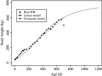
Modelling growth curves of animals is a common, useful tool for optimizing rearing management and thereby the efficiency of animal production. Studies on modelling growth curves have been published for pigs (Bastianelli & Sauvant Reference Bastianelli and Sauvant1997) and poultry (Aggrey Reference Aggrey2002), and Brown et al. (Reference Brown, Fitzhugh and Cartwright1976) compared different mathematical functions (logistic, Gompertz, von Bertalanffy, Brody and Richards functions) for representing body weight (BW) over time in different cattle breeds. These parametric models can fit average levels well, but ignore individual variations. In addition, they may not be fully relevant for heifers, because they require the asymptotic value of BW, i.e. adult BW at lactation 2 or 3. In practice, most animals are culled before lactation 4 (Seegers et al. Reference Seegers, Bareille and Beaudeau1998; Bell et al. Reference Bell, Wall, Russell, Roberts and Simm2010). Individual heifer BW seldom follows average theoretical growth curves (Fig. 1), because of variations induced by individual genetic potential, rearing strategies, health disorders, etc. From a practical point of view, these variations may be relevant: according to Ford & Park (Reference Ford and Park2001), a stepwise growth development of heifers, with a phase of energy restriction followed by re-feeding, should be encouraged for optimal milk yield. Traditional analysis as previously described thus appears to be of limited use for studying the impact of individual heifer BW variations on their subsequent performance.
Gompertz (GM; BW = 760 exp(–1·26 exp(–0·0036 × age))) and linear model (LM; BW = 54·76 + (0·77 × age)) adjustments applied to observed values from one heifer.

Spline functions have been proposed as alternatives to parametric models to model growth curves in cattle (Aggrey Reference Aggrey2002; Meyer Reference Meyer2005). Such semi-parametric (parametric by interval) methods generally improve the accuracy of most existing methods, taking into account growth dynamics between two ages of interest, and individual variability. Spline functions also allow the study of variations among animals and, using the first and second derivatives of the adjustment functions, studies on velocity and acceleration of BW curves are possible. With such an individual model of growth per animal, clustering into groups with similar growth dynamics and comparisons on the impact of growth profile on subsequent performance could be done on a large scale. Detecting and studying original growth profiles of interest from on-farm collected data would then be possible.
The aim of the present work was to develop new approaches for studying the impact of growth profile on subsequent performance, based on semi-parametric approximation of individual growth curves. Clustering methods were added to spline approaches to discriminate selected curve shapes. The impact of growth, and the velocity and the acceleration of such growth on dairy heifers and their yield performance during the first lactation were used to test the approach.
MATERIALS AND METHODS
Animals
Initial database
An initial database of 1391 Holstein heifers born between 1981 and 2006 was used. All the animals originated from an experimental herd of the Institut National de la Recherche Agronomique (INRA), located in western France (see Le Cozler et al. Reference Le Cozler, Peyraud and Troccon2009 for a more detailed description). In this herd, calvings were seasonal, and first calving occurred at either 24 or 36 months old. The database included BW of heifers, first lactation performance (milk yield and composition), reproduction data (heat, insemination and calving dates), information on health (treatment) and culling data. In the present study, only growth and first lactation performance was used, because most of the multiparous cows were included in other experiments after lactation 1, but the primiparous cows used in the present work were not used in those experiments.
Selection
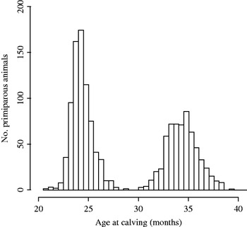
The description of the initial database indicated that 769 and 622 heifers first calved at c. 24 and 36 months old respectively (Fig. 2). To take the analysis further, selection was then performed as follows:
Number of animals per age at first calving in the original database (n = 1391).

During rearing, BW was recorded at least once every 4 months;
First calving occurred between 22·3 and 26·4 months old, which corresponded to mean age at first calving of the group of animals that first calved at c. 2 years of age (22·3 ± 2 times the value of the standard deviation). Only heifers first calving at 24 months old were kept, because it was impossible to determine precisely whether age 36 months at first calving was chosen, or resulted from poor growth or reproductive performance. This could alter the final results (Le Cozler et al. Reference Le Cozler, Peyraud and Troccon2009).
A final dataset of 447 heifers was used for the analysis of growth performance. A complementary analysis focused on 296 cows that completed a lactation period between 180 and 606 days.
In the experimental herd used in the present study, heifers were usually first turned out to pasture at 6–7 months old in special paddocks close to the weighing facility. This allowed regular measurement, every 3–4 weeks on average, similar to routine procedures performed when the herd was housed during winter. On the second turning out to pasture at, on average, 15–16 months old, heifers were already pregnant and moved to pasture paddocks, located in most cases far away from weighing facilities. In this case, BW was not measured regularly and measurements were sometimes taken only once or twice every 6 months, which is also a common practice in many commercial dairy herds. This resulted in missing weighing values from insemination until first calving (24 months old). However, since no trials or major changes in the management of the animals were performed during gestation in the period from 1981 to 2006, it was decided to analyse the impact of growth profiles from birth to insemination (15 months old) on subsequent performance.
Using spline methods
A spline is a piecewise polynomial function, made up of individual polynomial sections joined together at user-selected points called knot points. The function used performs cubic spline interpolation, i.e. spline with a polynomial function of order 3 (see formula below). This spline function must be continuously differentiable to order 4 at the inside points (the knot points).
The spline function for BW can be written as follows:
 $${\rm BW}(t) = \sum\limits_{\,j = 1}^k {{\rm} P_j (t)} = P_{\rm 1} (t) + P_{\rm 2} (t) + \ldots + P_j (t)$$
where
 $$P_j (t) = \sum\limits_{i = 0}^3 {{\rm} \alpha _{ij} t^i} = \alpha _{0j} + \alpha _{{\rm 1}j} t + \alpha _{{\rm 2}j} t^{\rm 2} + \alpha _{{\rm 3}j} t^{\rm 3} $$
BW is expressed in kg, t in days, and αij are the coefficients of the polynomial terms.
In this approach, the individual variability that results from short-term variation of BW can also be considered. This is of interest when automatic weighing systems perform several records per day, for example, or when animals are weighed several times per week, to study BW changes due to feed changes (e.g. turning out to pasture).
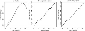
Different spline approaches were used and tested, as presented and discussed by Meyer (Reference Meyer2005). In a first step, comparisons between B-, smoothing- and interpolation-spline methods were made (Fig. 3). The B-spline approach requires several selected parameters to be set; otherwise automatic functions generate unrealistic parameters for several animals in the database. Similarly, the smoothing approach implies that at least one of these parameters is set. In practice, this parameter needs to be adapted for each curve, group of curves or, more generally, herd. This requires time, except if a specific algorithm is developed to determine this parameter automatically. In addition, B-spline and smoothing methods do not necessarily include all observations available in the database, resulting in some cases in possible looses of information regarding variability. Increasing frequency of collecting information would probably improve the final result, by using more of these available points. However, in practice, frequency of collected information varies a lot from animal to animal, farm to farm and even across years. The measurement frequency may then not be higher enough but increasing frequency may also lead to higher variations, resulting in some cases, in a higher number of false breakpoints. The aim was to find a method that would be easy to use in practice on in-farm collected data, and so such an approach appeared ill-suited. The interpolation spline method does not need any information to be set beforehand. It includes all the information available from the data, without exclusion, and it assumes there is no error in the data. It appeared to be the most relevant and so was selected for subsequent analysis.
The three spline approaches applied to observed values from one heifer. (a) B-spline method with 8 splines for the basis, and lambda = 10−5 (‘smooth.basisPar’ R-function in fda R-package); (b) cubic spline interpolation (‘spline’ R-function); and (c) smoothing splines (‘smooth.spline’ R-function).

In addition to analysis performed on growth profiles (i.e. BW changes over time, BW/time), this method was used to study velocity and acceleration of growth, which were calculated from first and second derivatives of the (BW/time) function. These parameters were estimated twice per month of age for animals, at the same age. Velocity and acceleration may be useful for the detailed growth study of dairy heifers, to determine the impact of rapid changes on short- or long-term performance.
Clustering the data
Two general clustering methods were applied and compared on results from spline interpolation adjustments (growth, velocity and acceleration curves).
Selecting a clustering method
The first clustering method tested was an agglomerative hierarchical clustering method, as described by Kaufman & Rousseeuw (Reference Kaufman and Rousseeuw1990). The number of clusters is chosen using a dendrogram analysis. When creating clusters, this method uses the Euclidean distances between objects, which are in fact the root sum-of-squares of differences. To initialize this algorithm, each created point is considered as a cluster in itself. The two nearest clusters are then combined to form a larger cluster and so on. At the end of the procedure, all of them are merged into one remaining cluster, which contains all the points. The linkage criterion determines the distance between hypothetical clusters. In this approach, the Ward criterion, based on the increasing variance for the clusters being merged, was used. This criterion is generally the best choice for functional data (Ferreira & Hitchcock Reference Ferreira and Hitchcock2009).
The second clustering method tested comprised two similar methods, the K-means and the partitioning around medoid (PAM) methods. The K-means method partitions the points into groups such that the sum of squares of the (points – assigned cluster centres) is minimized (MacQueen Reference MacQueen, le Cam and Neyman1967; Hartigan & Wong Reference Hartigan and Wong1979). In this case, all cluster centres represent the mean of the sets of data points nearest to each cluster centre, and the algorithm of Hartigan & Wong (Reference Hartigan and Wong1979) is used. Compared with the K-means method, the PAM algorithm is generally considered to be more robust because it minimizes the sum of the dissimilarities instead of the sum of the squared Euclidean distances (Kaufman & Rousseeuw Reference Kaufman and Rousseeuw1990). This algorithm consists of defining the representative medoids among the points of the dataset. Once they are found, clusters are built by assigning each point to the nearest medoid. The medoid of a cluster represents the central point of this cluster. Contrary to the calculated mean point, this point always exists in the cluster. For more information, please refer to Velmurugan & Santhanam (Reference Velmurugan and Santhanam2010).
Studying the irregularity of growth curves
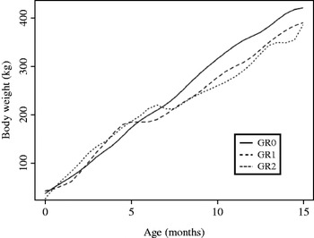
Growth is seldom linear and changes occur in growth shape (Figs 1 and 4). The relevance of breakdowns during rearing on subsequent performance was tested. In the present study, a breakdown existed only when the derivative of the interpolation function was negative or equal to zero. It could occur once or more during the period from birth to 15 months old. BW losses after birth are not uncommon in many species, such as humans, and sometimes 1–2 weeks are needed to observe resumed increase in BW. Thus, in the present study, the breakdowns during this period were not taken into account, since they could be considered as normal and natural phenomena. Animals were then finally classified according to the presence or absence of breakdowns, into three groups:
Gr0, for heifers with no breakdown in their growth from 0 to 15 months old;
Gr1, for heifers that experienced only one breakdown from 0 to 15 months old;
Gr2, for heifers whose growth curve presented at least two breakdowns from 0 to 15 months old.
Examples of three heifers growth without (Gr0) or with one (Gr1) or more than one (Gr2) breakdowns during the 0–15 months of age rearing period.

Statistical analysis
All calculations and analyses were performed using R Software (R Development Core Team 2012). The following available packages were used:
The ‘splines’ R-package, to perform the spline interpolation of weighing data. This package is part of the standard version of R software.
The ‘fda’ R-package for the B-spline smoothing (Ramsay & Silverman Reference Ramsay and Silverman2005). The function creates the spline basis with the number of splines selected by the user and the basis interval. Thereafter, the ‘smooth.basisPar’ function adjusts the real data to the basis.
The ‘cluster’ R-package to perform the PAM and hierarchical clusterings (Maechler et al. Reference Maechler, Rousseeuw, Struyf, Hubert and Hornik2012), K-means being a basic R-function directly available in R.
The performance of the different groups formed by clustering and/or breakdown approaches were evaluated using a Student's t test, completed by Welch modification when the variance between two samples was unequal (Welch Reference Welch1947). To study their impact on lactation performance, milk yield was calculated on a 305-day basis for all the cows, as described by Barbat et al. (Reference Barbat, Bonaiti and Boichard1995):
 $${\rm milk}\;{\rm 3}0{\rm 5}({\rm kg}) = {\rm total}\;{\rm milk}\;{\rm produced}\;({\rm kg}) \times ({\rm 385}/({\rm lactation}\;{\rm length}\;({\rm d}) + {\rm 8}0))$$
RESULTS
Average growth and/or lactation performance of primiparous cows used in the present analysis were consistent with previous results published by Le Cozler et al. (Reference Le Cozler, Peyraud and Troccon2009). As the present study focused more on methodological aspects, performance of animals will not be presented or discussed in detail until after the presentation of the results of the methodological approaches.
Modelling of growth curves
As described earlier in the present paper, the cubic spline interpolation method does not require any parameter to be fixed and better took into account the variability, whatever the frequency of measurement is, in comparison with other methods. Comparison of several spline methods showed that the cubic spline interpolation method, with no smoothing parameter to be chosen, was the best suited to the study of heifer growth (Fig. 3). This method emphasizes variations slightly, but it is better than the other two methods tested (B and Smooth), which eliminated them. Within the different B-splines method approaches tested, the 8 spline basis smoothed the curves too much, removing much of their variability. Increasing the number of base splines resulted in better accuracy of the fit, but the smoothing parameter, which varied from one animal to another, still had to be selected by the user. The smooth.spline function calculated by itself a smoothing parameter for each curve, but in many cases the result was not satisfactory visually.
Clustering methods and corresponding results
Selecting the most appropriate clustering method
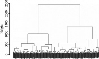
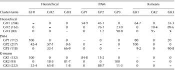
Similarly to previous analysis on growth modelling approaches, one method of clustering, PAM, appeared to be the most accurate to classify heifer growth into groups. In the tested methods, the number of groups was either fixed in advance (PAM and K-means) or selected (hierarchical). In the last case, the selection was based on a visual analysis of the dendrogram, which showed clusters of spots according to how closely they were correlated (Fig. 5). Three groups of heifer growth appeared to be the best choice, but the usefulness of two or four clusters was also tested and discussed. After interpolation of growth curves and clustering according to hierarchical, PAM and K-means methods, percent of heifers found in common between two groups from two different methods was determined (Table 1). Similar approaches were taken on velocity and acceleration databases, which originated from the initial database on growth values. Distribution of heifers in common according to methods (hierarchical (H), PAM (P) and K-means (K)) and selected item (growth (G), velocity (V) and acceleration (A)) is shown in Table 1.
Dendrogram of the hierarchical ascendant clustering method applied on growth values.

Percent of individuals in common in each group obtained by the different clusterings methods (in brackets, the number of animals per cluster) a. Growth curve analysis No. of observations in brackets. GH, GP, GK: groups of animals originating from hierarchical, PAM and K-means methods on growth (1–3: the three groups created within each of the applied methods). Data are considered exclusively on a line basis. For example, for GH1 and GP1: 54·9% of heifers in GH1 are also in GP1 and all GP1 are in GH1. b. Velocity No. of observations in brackets. VH, VP, VK: groups of animals originating from hierarchical, PAM and K-means methods on growth (1–3: the three groups created within each of the applied methods). Data are considered exclusively on a line basis. For example, for VP1 and VH1: 37·9% of heifers in VH1 are also in VP1 and 54·3% VP1 are in VH1. c. Acceleration No. of observations in brackets. AH, AP, AK: groups of animals originating from Hierarchical, PAM and K-means methods on growth (1–3: the three groups created within each of the applied methods). Data are considered exclusively on a line basis. For example, for AH1 and AP1: 28·3% of heifers in AH1 are also in AP1 and 95·3%AVP1 are in AH1.


In the hierarchical clustering method, the number of animals per group differed markedly when comparing growth, velocity and acceleration approaches (VH3, AH2 and AH3 had a limited number of observations). Similar results were noted for the K-means approach, particularly when considering acceleration (AK1 and AK2 groups). When using the PAM clustering method, no such variation was noted. Also, clustering analysis performed on velocity and acceleration gave similar average curves, although variations did not occur at the same age for all heifers. For further analysis, it was therefore decided to keep the three groups from the PAM approach.
Resulting animal performance analyses
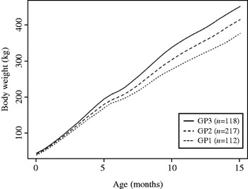
Growth performance from 0 to 15 months old within each of these three groups was significantly different (Fig. 6). BW was different in groups GP1, GP2 and GP3 at birth (39, 42 and 45 kg, respectively; P < 0·05) and 15 months old (376, 415 and 452 kg, respectively; P < 0·05). This corresponded to average daily gains (ADGs) of 684, 757 and 826 g/d, respectively (P < 0·05).
Changes in the BW in the three groups of animals GP1 (n = 112), GP2 (n = 217) and GP3 (n = 118), originating from the selected PAM method of clustering.

First lactation performance was studied on 296 cows with a lactation time of 314 (±53) d and varied from 185 to 606 days (Table 2a). Average milk yield on a 305-d basis was 6810 (±942) kg. Fat and protein content were 39·9 (±4·9) and 30·7 (±1·8) g/kg, respectively.
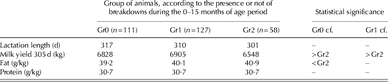
Average lactation performance for 296 primiparous cows that completed first lactation a. Overall performance b. According to growth profile during the 0–15 months of age period c. According to the presence or not of breakdowns during the 0–15 months of age period Animals in the GP1, GP2 and GP3 groups had an ADG from 0 to 15 months of age of 684, 757 and 826 g/d, respectively (P < 0·05). The three groups originated from the selected PAM method of clustering. Animals in the Gr0, Gr1 and Gr2 had 0, 1, or 2 or more breakdowns during the 0–15 months of age period.
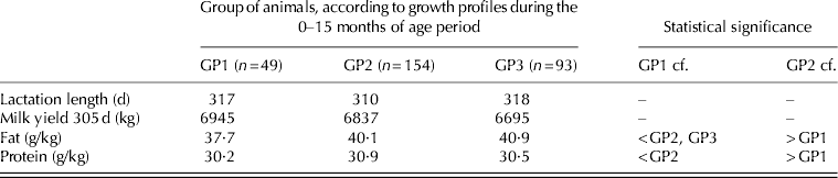
From the initial groups GP1, GP2 and GP3 created from rearing data, this represented 49, 71 and 79% of the initial numbers of animals, respectively (Table 2b). Neither milk yield on a 305-d basis nor lactation length was affected by group. Heifer milk from GP1 contained less fat than GP2 or GP3 heifer milk (37·7 v. 40 or more g/kg, respectively; P < 0·05) and less protein (30·2 and 30·5 or more g/kg, respectively; P < 0·05).
Similar approaches, based on clustering animals according to velocity and acceleration of their growth curves, showed no difference in performance, during either rearing or lactation (not presented).
Relevance and possible importance of breaks
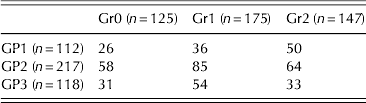
A total of 125 animal curves had no breakpoints from 0 to 15 months old, while 175 had only one breakpoint and 147 had two or more: only 33 animals displayed three breakpoints or more. The study on the impact of breakpoints during growth on subsequent performance was performed on the 296 animals on which lactating performance was studied (Table 2c). When more than two breakpoints were noted, milk yield on a 305-d basis was reduced significantly (6548 v. 6828 and 6905 kg, for Gr2, Gr1 and Gr0 animals, respectively). Fat content was also higher in group Gr2 than in Gr0, but overall, no difference in total fat or protein-corrected milk production was noted. Experiencing two breaks or more during growth thus appeared to have an adverse effect on subsequent performance. The intersection between groups for growth and groups for breakdowns confirmed that animals that had two breakdowns or more belonged more frequently to the group that had the lowest growth performance (GP1), whereas a higher proportion of animals with only one break were found in groups GP2 and GP3 (Table 3).
Distribution of the 447 animals according to growth profiles and presence or not of breakdowns during the 0–15 months of age period
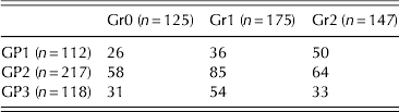
Animals in the Gr0, Gr1 and Gr2 had 0, 1, or 2 or more breakdowns during the 0–15 months of age period.
Animals in the G1, G2 and G3 groups had an ADG from 0 to 15 months of age of 684, 757 and 826 g/d, respectively (P < 0·05). The three groups originated from the selected PAM method of clustering.
DISCUSSION
Animal performance: comparison between methods
The results concerning the performance of the animals were as expected and in close agreement with earlier published results (Le Cozler et al. Reference Le Cozler, Peyraud and Troccon2009). The difference between ADG levels in each group created with the non-parametric method and the classification were probably not high enough to observe any adverse effects of excessive growth rate on performance during lactation one (Le Cozler et al. Reference Le Cozler, Lollivier, Lacasse and Disenhaus2008). This was particularly so for the high growth rate group (GP3 with an ADG of 826 g/d from 0 to 15 months old). However, the low ADG during rearing had similar yield performance, but fewer animals performed a normal first lactation, meaning that they were culled more frequently. Although not precisely analysed, this could be a result of inadequate lactation performance, reproduction performance or problems at calving. As the present work aimed at testing and discussing the utility of new methods of growth analysis, the results from impact of ADG before insemination on subsequent performance during lactation will not be discussed further.
Non-parametric approach
In a management information system dealing with events such as reproductive or health events, real-time smoothing is of importance, since in most cases events require immediate responses. Real-time analysis methods based on Kalman filters, for example (De Mol et al. Reference De Mol, Keen, Kroeze and Achten1999), are therefore relevant in these instances. In long-term and/or historical approaches (genetic or growth aspects, for example), delaying analysis for several hours, days or even months is possible and consequently, using real-time methods is not necessary and non-parametric approaches based on splines analysis are then of interest.
Spline approaches have been used for decades not only in industry but also in animal sciences, especially by geneticists (Meyer Reference Meyer2005), but not exclusively (Codrea et al. Reference Codrea, Hojsgaard and Friggens2011). The use of non-linear methods to analyse heifer growth offers new opportunities to study the relevance of variability in individual profiles precisely and to explore large databases. The cubic spline interpolation method appeared to be the most useful and best-suited of the different spline method tested to model growth of dairy rearing heifers. One of its main strengths is that data can be used with missing values and irregular records. In contrast, the B-splines method is useful when measurement frequency is high and regular, with few missing values. For example, Codrea et al. (Reference Codrea, Hojsgaard and Friggens2011) used this method successfully to detect short-term disturbance in milk yield, where measurements are taken more than once a day. The B-Spines method could be used for growth, but it requires growth performance to be recorded frequently. In agencies tasked with tracking animal growth in commercial farms, weighing of animals may not be regular. In some cases, especially during the grazing season, many animals are not weighed, resulting in missing information.
The relevance of velocity and acceleration were tested, as suggested by Robert et al. (Reference Robert, Tessier and Martin2010), who indicated that these aspects could be of interest when studying kinetic processes from functional data analysis (FDA). However, neither velocity nor acceleration had any impact on performance. This approach may not be well-suited or useful for analyses based on data recorded no more than once per month. It is probably better suited to data collected daily or weekly, such as milk production, thanks to new technology being developed in farms, such as milking robots or new milk meters within traditional milking systems. The variability that exists between animals could then be studied and changes in the velocity and/or acceleration of the milking curves could be connected with health aspects, for example (Codrea et al. Reference Codrea, Hojsgaard and Friggens2011).
Utility of modelling growth profiles with non-parametric approaches
Studying heifer growth is generally aimed at establishing recommendations or re-adapting inadequate rearing programmes. In such cases, users generally refer to BW at a fixed age (e.g. 6 or 24 months) or to an ADG during a period (e.g. 6–24 months; Wattiaux Reference Wattiaux1997), but very little information is available on what is the best growth profile to achieve this. To meet such targets, different growth profiles may exist and growth is seldom linear. Ford & Park (Reference Ford and Park2001) published results that showed that non-linear profiles were more useful than linear ones. However, although pre-planned experiments on a limited number of animals makes this approach possible, it is hard to analyse results collected from a large database, where original and useful growth profiles may exist. Developing approaches and analysis that could take into account this fact is thus of importance.
Occurrence of one breakpoint from birth to insemination showed no effect on milking performance, whereas two breakpoints or more resulted in reduced milking yield during lactation one. Ford & Park (Reference Ford and Park2001) have shown beneficial effect of non-linear growth on subsequent milking performance of cows first calving at 24 months of age. But Le Cozler et al. (Reference Le Cozler, Peccate and Delaby2010, Reference Le Cozler, Gallard, Dessauge, Peccate, Trommenschlager and Delaby2011), in experiments where cows first calved at 36 months old, noted that resulting breakdowns from restricted growth during winter were more pronounced when they occurred during two successive winter housing seasons compared to during only one. This suggests that the negative effect of one breakpoint could be counterbalanced but, in case of two breakpoints or more, it may not be possible. However, only negative breakpoints during rearing have been considered in the present study, but the interest of positive breakpoints remains to be studied. Further investigations on these aspects and approaches are needed in the future.
Possible further improvement of the approach
The impact of season of birth could not be studied in the present work, since calvings were seasonal in the experimental herd. In a preliminary study, the results indicated a limited impact of year of birth on growth profile. After classification, analysis showed that animals within each group originated equally from the different year of birth, which partially justified that fact that it was not included in the statistical analysis. However, it is highly probable that analysis on larger datasets from different herds require its inclusion. Similarly, no genetic aspect (dam or sire) was considered, mainly because of the limited number of animals. And in this particular case of genetic approaches, the spline methods have already been used successfully, as presented and discussed by Meyer (Reference Meyer2005).
The approaches developed in the present paper could be used not only on BW data but also on body score index, girth development or other growth parameters. The method may also be used for variables other than growth, such as, milk yield or BW variation during lactation. Using these approaches to study longevity or reproductive/productive performance on non-experimental animals would be of interest. It could be performed on data from herds in which animals are tracked through both growth and milk quality control, which represents a valuable source of information. The utility of such an approach has also to be considered in other animal production systems, such as dairy goats or beef cattle. Overall, it may open up opportunities to develop new models for predicting the probability of heat appearance on an animal basis, which could be included among useful management tools.
CONCLUSION
The present study tested and used semi-parametric methods to study the impact of heifer growth from 0 to 15 months old on their first lactation performance, taking into account the variability of growth profiles. Although performed on a database originating from one herd, with one breed and small variations in rearing strategies, this approach offers interesting and promising opportunities for analysing larger databases, originating from several herds, with different breeds. It also allows extraction of useful features from low frequency life-weight measurements during the growing period to predict further performance. And finally, it may open opportunities for developing new guidelines and tools in the future for optimal rearing of dairy heifers.
The authors thank the Region of Brittany and INRA for funding the PhD Scholarship of Cecile Sauder.