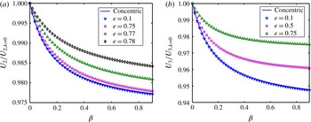
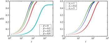
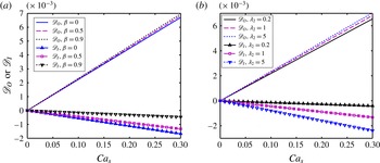
1 Introduction
The dynamics of ‘compound droplets’ or ‘double emulsions’ has been an area of extensive research for a long time, mainly attributable to its wide spectrum of applications (Garti & Bisperink Reference Garti and Bisperink1998), starting from materials processing (Lee Reference Lee2001; Sapei, Naqvi & Rousseau Reference Sapei, Naqvi and Rousseau2012) to the modelling of blood cells (Kan et al. Reference Kan, Udaykumar, Shyy and Tran-Son-Tay1998). A compound droplet is essentially defined as a liquid drop, completely engulfed within a second immiscible drop, and the second drop itself is suspended within a third immiscible medium. These kinds of arrangements physically occur in many processes, some of which include phase separation (Draxler & Marr Reference Draxler and Marr1986), oil recovery through porous structures (Stone & Leal Reference Stone and Leal1990a ), formation of lipid bilayers (Palaniappan & Daripa Reference Palaniappan and Daripa2000) and drug delivery (Nakano Reference Nakano2000; Fabiilli et al. Reference Fabiilli, Lee, Kripfgans, Carson and Fowlkes2010), to name a few. Various aspects of the dynamics of compound droplets have been extensively studied (Johnson & Sadhal Reference Johnson and Sadhal1985; Sadhal & Oguz Reference Sadhal and Oguz1985; Sadhal, Ayyaswamy & Chung Reference Sadhal, Ayyaswamy and Chung1996; Tsemakh, Lavrenteva & Nir Reference Tsemakh, Lavrenteva and Nir2004) over the past couple of decades. These studies include the behaviour of rigid compound droplets in quiescent flows (Torza & Mason Reference Torza and Mason1970), deformation and breakup of compound droplets in linear flows (Davis & Brenner Reference Davis and Brenner1981; Smith, Ottino & Olvera de la Cruz Reference Smith, Ottino and Olvera de la Cruz2004; Chen, Liu & Shi Reference Chen, Liu and Shi2013; Hua, Shin & Kim Reference Hua, Shin and Kim2014; Chen et al. Reference Chen, Liu, Zhang and Zhao2015a ), dynamics of double emulsions in the presence of electric fields (Gouz & Sadhal Reference Gouz and Sadhal1989; Ha & Yang Reference Ha and Yang1999; Behjatian & Esmaeeli Reference Behjatian and Esmaeeli2013, Reference Behjatian and Esmaeeli2015) and thermocapillary action (Morton, Subramanian & Balasubramaniam Reference Morton, Subramanian and Balasubramaniam1990; Borhan, Haj-Hariri & Nadim Reference Borhan, Haj-Hariri and Nadim1992), compound droplets in parabolic flows (Haj-Hariri, Nadim & Borhan Reference Haj-Hariri, Nadim and Borhan1993), gravitational settling of double emulsions (Rushton & Davies Reference Rushton and Davies1983; Sadhal & Oguz Reference Sadhal and Oguz1989), and many more (Johnson & Sadhal Reference Johnson and Sadhal1985; Sadhal et al. Reference Sadhal, Ayyaswamy and Chung1996). We note that, while a number of the aforementioned studies have been executed only for concentric drops, a handful of studies (Sadhal & Oguz Reference Sadhal and Oguz1985; Morton et al. Reference Morton, Subramanian and Balasubramaniam1990; Tsemakh et al. Reference Tsemakh, Lavrenteva and Nir2004; Qu & Wang Reference Qu and Wang2012) have also focused on the dynamics of eccentric compound droplets. Previously, Sadhal and coworkers (Johnson & Sadhal Reference Johnson and Sadhal1985; Sadhal & Oguz Reference Sadhal and Oguz1985; Oguz & Sadhal Reference Oguz and Sadhal1987) have probed the motion of eccentric double emulsions under gravitational forcing. In addition to this, Tsemakh et al. (Reference Tsemakh, Lavrenteva and Nir2004) have also studied the motion of eccentric double emulsions in the presence of soluble surfactants. Song, Xu & Yang (Reference Song, Xu and Yang2010) have numerically studied the motion of eccentric compound drops in a circular tube, the background flow being Poiseuille in nature. Morton et al. (Reference Morton, Subramanian and Balasubramaniam1990) have investigated thermocapillary migration of compound drops towards solid surfaces.
It has long been agreed upon in the literature that multiphase systems often have surfactants, or surface active agents (Stone & Leal Reference Stone and Leal1990b ), present as impurities (or sometimes even as additives). For example, Pal (Reference Pal2007) has reported the necessity to use surfactants in order to form double emulsions. These substances are generally adsorbed at the interface between the liquid phases and have been shown to have strong effects on the interfacial properties (Stone & Leal Reference Stone and Leal1990b ; Schwalbe et al. Reference Schwalbe, Phelan, Vlahovska and Hudson2011), especially the interfacial tension. Therefore, the presence of surfactants can bring about significant alterations to the dynamics and deformations of a drop, through altering the interfacial properties. A wide range of previously executed studies (Stone & Leal Reference Stone and Leal1990b ; Blawzdziewicz, Vlahovska & Loewenberg Reference Blawzdziewicz, Vlahovska and Loewenberg2000; Vlahovska, Blawzdziewicz & Loewenberg Reference Vlahovska, Blawzdziewicz and Loewenberg2002; Vlahovska, Bławzdziewicz & Loewenberg Reference Vlahovska, Bławzdziewicz and Loewenberg2009; Vlahovska Reference Vlahovska2011) have investigated the dynamics of surfactant laden droplets, for a variety of flow conditions. Stone & Leal (Reference Stone and Leal1990b ) showed that, generally, under the limit of low capillary number (Ca), surfactants tend to augment droplet deformations. Similar results were also obtained later by Vlahovska and coworkers (Blawzdziewicz et al. Reference Blawzdziewicz, Vlahovska and Loewenberg2000; Vlahovska et al. Reference Vlahovska, Blawzdziewicz and Loewenberg2002; Vlahovska, Loewenberg & Blawzdziewicz Reference Vlahovska, Loewenberg and Blawzdziewicz2005; Vlahovska et al. Reference Vlahovska, Bławzdziewicz and Loewenberg2009). More recent studies (Hanna & Vlahovska Reference Hanna and Vlahovska2010; Schwalbe et al. Reference Schwalbe, Phelan, Vlahovska and Hudson2011; Pak, Feng & Stone Reference Pak, Feng and Stone2014) have shown that advection of surfactants on a drop interface leads to cross-stream migration of the spherical droplet in the presence of background Poiseuille flow. A relatively smaller number of studies (Morton et al. Reference Morton, Subramanian and Balasubramaniam1990; Borhan et al. Reference Borhan, Haj-Hariri and Nadim1992; Haj-Hariri et al. Reference Haj-Hariri, Nadim and Borhan1993; Tsemakh et al. Reference Tsemakh, Lavrenteva and Nir2004; Rosenfeld, Lavrenteva & Nir Reference Rosenfeld, Lavrenteva and Nir2009; Lavrenteva, Rosenfeld & Nir Reference Lavrenteva, Rosenfeld and Nir2011) have also been executed to investigate the effects of surfactant on compound drop systems. These include thermocapillary migration of compound drops in the presence of surfactants (Morton et al. Reference Morton, Subramanian and Balasubramaniam1990; Borhan et al. Reference Borhan, Haj-Hariri and Nadim1992; Haj-Hariri et al. Reference Haj-Hariri, Nadim and Borhan1993; Rosenfeld et al. Reference Rosenfeld, Lavrenteva and Nir2009; Lavrenteva et al. Reference Lavrenteva, Rosenfeld and Nir2011) and locomotion of double emulsions in the presence of surfactant secretion (as already mentioned, see Tsemakh et al. (Reference Tsemakh, Lavrenteva and Nir2004)), to name a few.
A wide range of previous studies (Schowalter, Chaffey & Brenner Reference Schowalter, Chaffey and Brenner1968; Frankel & Acrivos Reference Frankel and Acrivos1970; Raja, Subramanian & Koch Reference Raja, Subramanian and Koch2010; Oliveira & Cunha Reference Oliveira and Cunha2011; Subramanian et al. Reference Subramanian, Koch, Zhang and Yang2011; Ramachandran & Leal Reference Ramachandran and Leal2012; Faroughi & Huber Reference Faroughi and Huber2015) have further investigated the overall rheological behaviour, as shown by a dilute solution of droplets and particles, based on the method prescribed by Batchelor (Batchelor Reference Batchelor1970; Batchelor & Green Reference Batchelor and Green1972a ,Reference Batchelor and Green b ) and Einstein (Leal Reference Leal2007). The effects of various physical quantities on the ‘effective viscosity’ of a dilute suspension in a linear flow have been rigorously analysed, including the effect of interfacial slip (Ramachandran et al. Reference Ramachandran, Tsigklifis, Roy and Leal2012; Ramachandran & Leal Reference Ramachandran and Leal2012), the effect of surfactants (Vlahovska et al. Reference Vlahovska, Blawzdziewicz and Loewenberg2002) and the effect of electric field (Vlahovska Reference Vlahovska2011), to name a few. Vlahovska et al. (Reference Vlahovska, Blawzdziewicz and Loewenberg2002) have shown that the presence of surfactants, in conjunction with a deformed drop shape, leads to non-Newtonian type behaviours of dilute suspensions. Previously, Stone & Leal (Reference Stone and Leal1990a ) deduced the effective viscosity of a dilute suspension of compound drops and demonstrated that the system behaves like a suspension of rigid particles as the inner droplet radius closely approaches that of the outer one. A number of experimental studies on the rheological properties of droplet suspensions (Pal Reference Pal1996a ,Reference Pal b , Reference Pal2007; Rust & Manga Reference Rust and Manga2002) have also been reported in the literature. These investigations demonstrate that the suspensions can show a wide range of rheological behaviour, starting from Newtonian behaviour for dilute suspensions (Pal Reference Pal2007) to shear thinning properties for concentrated ones (Frith, Mewis & Strivens Reference Frith, Mewis and Strivens1987). Pal (Reference Pal1996a ,Reference Pal b , Reference Pal2007, Reference Pal2008), among others, has executed several experiments on the rheology of suspensions of double emulsions, with varying degree of droplet concentration. His experiments revealed that the constitutive behaviour depends strongly on the droplet viscosities as well as the volume fraction. On the other hand, most theoretical studies on double emulsions have been executed either for axisymmetric flows or in linear flows, usually ignoring the effects of surfactants. In this regard it should be noted that Matsumoto and coworkers (Kita, Matsumoto & Yonezawa Reference Kita, Matsumoto and Yonezawa1977; Matsumoto & Kohda Reference Matsumoto and Kohda1980) have proposed an empirical relation, also known as Mooney’s relation (Pal Reference Pal2007), which can be used to predict the viscosity of double/multiple emulsions. Finally, we infer from a close review of the concerned literature that the dynamics and deformation of a compound droplet (concentric as well as eccentric) system in an arbitrary Stokes flow in the presence of surface active agents are yet to be extensively addressed in the literature.
Here, we attempt to analyse the dynamics and deformation of a compound drop system, residing in an unbounded arbitrary Stokes flow, with surfactants being present on both of the interfaces. Our analysis can be divided into two main sections. First, we take up the cases of concentric surfactant laden drops, subjected to arbitrary far-field (Stokes) flows. We employ Lamb’s solutions (Lamb Reference Lamb1975; Kim & Karrila Reference Kim and Karrila1991) and derive the resulting flow fields, drop velocity, drop deformation and surfactant concentration. Our calculations also furnish the corresponding drop velocities. We infer that the assumption of the concentric drop situation easily breaks down, as soon as the two drops start to move at different velocities. Therefore, we apply our analysis for concentric drops to two special and practically relevant cases, namely (i) uniaxial extensional flows and (ii) shear flows. Since none of these flows result in any droplet migration velocities, concentric droplets remain concentric at all times. We further deduce the effective viscosity of a dilute suspension of double emulsions in uniaxial extensional as well as shear flows, in the presence of surfactants. We subsequently compare our analytical findings with the previously derived expressions of Stone & Leal (Reference Stone and Leal1990a
) and find exact agreement. We further compare our theoretical predictions of suspension viscosity with the previously reported theory and experiments of Pal (Reference Pal2007), and demonstrate that better agreement between theory and experiments can be observed when the effects of surfactants are taken into account. Nevertheless, for many other kinds of flows (for example settling) the assumption of concentric drops quickly breaks down, rendering the previous solutions inapplicable. In light of this shortcoming, the second part of the analysis is dedicated to the study of the motion of surfactant laden eccentric compound drop systems in axisymmetric but otherwise arbitrary Stokes flows (one example is Poiseuille flow). We assume the eccentricity to be arbitrary and employ a bipolar coordinate system (Brenner Reference Brenner1961; Happel & Brenner Reference Happel and Brenner1981) to work out the velocity and surfactant distribution in and around the droplets. Although our analysis is fairly general and can be used to study any axisymmetric flow, here we probe the Poiseuille flow, as a representative example, and study the effects of eccentricity in conjunction with surfactant concentration on the streamwise migration velocity of droplets. In our derivations, we assume the capillary number to remain small enough that the drops can be approximated as spheres and deduce only the leading-order flow fields, drop velocities and the resulting
 $O(Ca)$
deformations. In an effort to maintain focus and to avoid confusion, we consider the surfactant to be insoluble in the bulk. It should be noted that a number of previous studies (Stone & Leal Reference Stone and Leal1990b
; Ha & Yang Reference Ha and Yang1995; Leal Reference Leal2007) have made such assumptions in order to preserve simplicity.
The central finding of our analysis is that, in linear flows, the presence of surfactant always increases the deformation of the inner drop, whereas, for the outer drop, the relative change in the deformation depends strongly on the ratio of the radii of the two droplets. We further demonstrate that the presence of surfactants generally causes the effective viscosity of a dilute suspension of compound drops to increase, when subjected to linear flows. Our results reveal that, in the case of Poiseuille flows, the inner drop usually moves faster compared with the outer drop, which naturally results in an ever-increasing eccentricity. However, the relative velocity of the inner drop keeps on decreasing as it nears the interface of the outer drop. We subsequently compare our results for droplet migration velocities in Poiseuille flow from the two analyses (concentric and eccentric theories) and show that significant deviation can only be observed for relatively large values of the eccentricity.
2 System description and governing equations
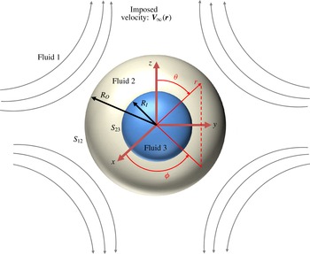
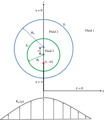
Schematics of the physical system under consideration for the present analysis are depicted in figures 1 (for concentric drops) and 2 (for eccentric drops). The eccentricity (
 $e$
) is defined as the distance between the centres (refer to figure 2) of the two drops. We consider a ‘compound drop’ system, where the outer drop has a radius
 $R_{O}$
and the inner drop radius is
 $R_{I}$
. We attach our coordinate system to the outer drop and place the origin at the centre of the concentric drop system, as shown in the above schematic. For an eccentric drop system (refer to figure 2), we employ a bipolar coordinate system, wherein the frame of reference is still attached to the outer drop centre, but the origin lies beneath the drops. We denote the outermost phase (the suspending medium) by 1, the outer drop phase by 2 (the shell region) and the innermost phase by 3, and use these numbers in subscripts to denote various properties. More specifically, we denote the viscosity of the
 $i$
th fluid by
 $\unicode[STIX]{x1D707}_{i}$
, the density by
 $\unicode[STIX]{x1D70C}_{i}$
, while the interface between the
 $i$
th and
 $j$
th fluids is denoted by subscript ‘
 $ij$
’. Following this notation, the interfacial tension is denoted by
 $\unicode[STIX]{x1D70E}_{ij}$
. We further consider surfactants to be present in the system, which are insoluble in the bulk and only get adsorbed at the interface (Stone & Leal Reference Stone and Leal1990b
). The surfactant concentration at the
 $ij$
th interface is denoted by
 $\unicode[STIX]{x1D6E4}_{ij}$
, while the equilibrium concentration of the same is denoted as
 $\unicode[STIX]{x1D6E4}_{ij}^{0}$
. The corresponding interfacial tension is assumed to follow a linear relationship with the surfactant concentration, which is given by (Stone & Leal Reference Stone and Leal1990b
; Pak et al.
Reference Pak, Feng and Stone2014)
 $\unicode[STIX]{x1D70E}_{ij}=\unicode[STIX]{x1D70E}_{ij}^{0}-R_{g}T\unicode[STIX]{x1D6E4}_{ij}$
, where
 $\unicode[STIX]{x1D70E}_{ij}^{0}$
is the interfacial tension in the absence of surfactants,
 $R_{g}$
is the ideal gas constant and
 $T$
is the absolute temperature of the system. We assume the flow at a large distance from the drop centre to be
 $\boldsymbol{V}_{\infty }$
, which obeys the Stokes flow equations, but is otherwise arbitrary in nature. Additionally, the outer and inner drops are assumed to move at velocities
 $\boldsymbol{U}_{2}$
and
 $\boldsymbol{U}_{3}$
respectively, which, in general, are different and will be obtained as part of the solution. A few other assumptions are made for the present study. We briefly mention them before we move towards the detailed formulation.
First, we assume that all flows obey the Stokes equations, i.e. the Reynolds number in each phase is far less than unity. Second, the drops are assumed to remain approximately spherical. We note that drop deformation in the limits of creeping flows is strongly dictated by the magnitude of the capillary number (
 $Ca=\unicode[STIX]{x1D707}u_{c}/\unicode[STIX]{x1D70E}$
) when the viscosity of any phase is of same order of magnitude as other phases. Here,
 $u_{c}$
is the characteristic velocity, defined later. Therefore, a low magnitude of
 $Ca$
(i.e.
 $Ca\ll 1$
) would eventually lead to small deformations, wherein the drops can be assumed to stay nearly spherical. Third, the flow is assumed to remain quasi-steady at all times. Since the droplets would move with different velocities in a general far-field flow, this would naturally lead to temporal evolution of the whole compound drop configuration. The assumption of low Reynolds number and quasi-steady flow enables us to neglect the temporal derivative on the left-hand side of the Navier–Stokes equations. As a result, the fluid motion at a given time becomes a function of the instantaneous location of the droplets. It should be noted that the assumption of quasi-steady flow while studying the creeping motion of droplets is abundant in the literature, for example Ramachandran & Leal (Reference Ramachandran and Leal2012), Pak et al. (Reference Pak, Feng and Stone2014) and Mandal, Bandopadhyay & Chakraborty (Reference Mandal, Bandopadhyay and Chakraborty2015). Fourth, the double emulsion system is assumed to remain stable. Previously, Stone & Leal (Reference Stone and Leal1990a
) have shown that for large values of
 $Ca$
, the drops can break up, leading to unstable configurations. However, in the present study, we assumed that the double emulsions remain stable at all times. Notably, recent experimental studies (Ficheux, Bonakdar & Bibette Reference Ficheux, Bonakdar and Bibette1998; Utada et al.
Reference Utada, Lorenceau, Link, Kaplan, Stone and Weitz2005; Pal Reference Pal2007; Kim et al.
Reference Kim, Kim, Cho and Weitz2011) on the generation of double emulsions have shown that using novel techniques, such as actuating bi-phase flow in narrow capillaries (Kim et al.
Reference Kim, Kim, Cho and Weitz2011), one can generate very stable double emulsions, even when the shell-drop thickness (phase 2) is very small (submicron range). Moreover, the methods employed in these studies have further been shown to offer a high degree of control over droplet sizes. In an earlier study, Ficheux et al. (Reference Ficheux, Bonakdar and Bibette1998) have looked into the criterion for instability of double emulsions. Their experimental results showed that, depending on the surfactant concentration, the time scale of instability and collapse of the double emulsions can be varied from several months to even minutes. In addition to this, it has also been shown (Leal Reference Leal2007) that the presence of surfactants (as considered in this analysis) on the droplet interfaces may augment the stability of emulsions by creating a barrier for droplet coalescence. In fact, this is one of the reasons why surfactants are used as emulsifiers to stabilize droplet suspensions. For more details on the generation and stability of double emulsions, one can refer to the work of Ficheux et al. (Reference Ficheux, Bonakdar and Bibette1998), Utada et al. (Reference Utada, Lorenceau, Link, Kaplan, Stone and Weitz2005) Pal (Reference Pal2007), and Kim et al. (Reference Kim, Kim, Cho and Weitz2011). Fifth, it is important here to justify the assumption of bulk-insoluble surfactants. Although surfactants are usually soluble in the bulk, their most dominant effect on droplet motion occurs due to their presence on the interfaces. An important limiting case in this regard occurs (Leal Reference Leal2007) when the convection at the interface is very fast compared with the bulk diffusion or adsorption desorption kinetics. This can be quantified as (Leal Reference Leal2007)
 $Bi\ll 1$
, where
 $Bi$
is the surfactant Biot number, expressed as
 $Bi=\unicode[STIX]{x1D705}R_{O}/u_{c}$
,
 $\unicode[STIX]{x1D705}$
being the desorption rate and
 $u_{c}$
being the characteristic velocity, defined later. This physical paradigm is sometimes referred to as the ‘insoluble’ limit, wherein the surfactant kinetics at the interface is decoupled from that in the bulk, at least as a first approximation. For further details on surfactant kinetics and bulk-insoluble surfactants, one can refer to the book of Leal (Reference Leal2007, chap. 7). Finally, we note that the formulation in this section is quite general and can be applied to any coordinate system.
The equation of fluid motion for the
 $i$
th (
 $i=1,2,3$
) fluid is given by
 $$\begin{eqnarray}\unicode[STIX]{x1D707}_{i}\unicode[STIX]{x1D6FB}^{2}\boldsymbol{u}_{i}-\unicode[STIX]{x1D735}p_{i}=\mathbf{0},\quad \unicode[STIX]{x1D735}\boldsymbol{\cdot }\boldsymbol{u}_{i}=0.\end{eqnarray}$$
Equations (2.1) are subjected to the following far-field boundary condition:
 $$\begin{eqnarray}\text{as}~r\rightarrow \infty ,\quad \boldsymbol{u}_{1}\rightarrow \boldsymbol{V}_{\infty }-\boldsymbol{U}_{2}.\end{eqnarray}$$
The interfacial conditions are given by the usual no-slip, no-penetration and stress balance (in steady state) conditions. These conditions read, on the interface
 $S_{ij}$
,
 $$\begin{eqnarray}\displaystyle & \displaystyle [\boldsymbol{u}_{i}]_{S_{ij}}=[\boldsymbol{u}_{j}]_{S_{ij}}, & \displaystyle\end{eqnarray}$$
 $$\begin{eqnarray}\displaystyle & \displaystyle [\boldsymbol{u}_{i}\boldsymbol{\cdot }\boldsymbol{n}_{ij}]_{S_{ij}}=[\boldsymbol{u}_{j}\boldsymbol{\cdot }\boldsymbol{n}_{ij}]_{S_{ij}}=(\boldsymbol{U}_{3}-\boldsymbol{U}_{2})\boldsymbol{\cdot }\boldsymbol{n}_{23}\unicode[STIX]{x1D6FF}_{i2}\unicode[STIX]{x1D6FF}_{j3}, & \displaystyle\end{eqnarray}$$
 $$\begin{eqnarray}\displaystyle & \displaystyle [\unicode[STIX]{x1D749}_{i}\boldsymbol{\cdot }\boldsymbol{n}_{ij}]_{S_{ij}}-[\unicode[STIX]{x1D749}_{j}\boldsymbol{\cdot }\boldsymbol{n}_{ij}]_{S_{ij}}=\unicode[STIX]{x1D70E}_{ij}(\unicode[STIX]{x1D735}_{s}\boldsymbol{\cdot }\boldsymbol{n}_{ij})\boldsymbol{n}_{ij}-\unicode[STIX]{x1D735}_{s}\unicode[STIX]{x1D70E}_{ij}. & \displaystyle\end{eqnarray}$$
Here, we have used a generic notation
 $[~]_{S_{ij}}$
to represent the evaluation of the inside quantity at the surface
 $S_{ij}$
. It should be noted that, in (2.4),
 $\unicode[STIX]{x1D6FF}_{ij}$
denotes the Kronecker delta tensor and
 $\boldsymbol{n}_{ij}$
is the outward unit normal to the interface
 $S_{ij}$
(
 $\boldsymbol{n}_{ij}=\unicode[STIX]{x1D735}F_{ij}/|\unicode[STIX]{x1D735}F_{ij}|$
,
 $F_{ij}$
being the equation of the surface). In (2.5),
 $\unicode[STIX]{x1D749}_{i}$
is the stress tensor in the
 $i$
th fluid and is given by
 $\unicode[STIX]{x1D749}_{i}=-p_{i}\unicode[STIX]{x1D644}+\unicode[STIX]{x1D707}_{i}[\unicode[STIX]{x1D735}\boldsymbol{u}_{i}+(\unicode[STIX]{x1D735}\boldsymbol{u}_{i})^{\text{T}}]$
, whereas
 $\unicode[STIX]{x1D735}_{s}=[\unicode[STIX]{x1D735}-\boldsymbol{n}_{ij}(\boldsymbol{n}_{ij}\boldsymbol{\cdot }\unicode[STIX]{x1D735})]$
represents the surface gradient operator. In addition to the aforementioned equations, we have to consider additional conservation equations for the surface active agents on the interfaces. These are essentially surface conservation equations, which take into account surface diffusion and surface advection of the surfactants. On interface
 $S_{ij}$
, the surfactant transport equation at steady state reads (Stone Reference Stone1990; Stone & Leal Reference Stone and Leal1990b
):
 $$\begin{eqnarray}\unicode[STIX]{x1D735}_{s}\boldsymbol{\cdot }(\boldsymbol{u}_{S_{ij}}\unicode[STIX]{x1D6E4}_{ij})=D_{ij}\unicode[STIX]{x1D6FB}_{s}^{2}\unicode[STIX]{x1D6E4}_{ij},\end{eqnarray}$$
where
 $D_{ij}$
denotes the surface diffusivity of the surfactants. In (2.6),
 $\boldsymbol{u}_{S_{ij}}=[\boldsymbol{u}_{i}]_{S_{ij}}$
denotes the fluid velocity on
 $S_{ij}$
.
At this stage, it is important to note that fluid–fluid interfaces can show a host of complex rheological properties (Flumerfelt Reference Flumerfelt1980; Pozrikidis Reference Pozrikidis2001; Schwalbe et al. Reference Schwalbe, Phelan, Vlahovska and Hudson2011; Gounley et al. Reference Gounley, Boedec, Jaeger and Leonetti2016) in the presence of surface active agents. However, it is widely accepted that clean interfaces and surfaces with single layers of surfactants are in general isotropic in nature (Pozrikidis Reference Pozrikidis2001). However, the presence of structures on interfaces, for example the presence of adsorbed proteins (Dickinson Reference Dickinson1999; Wilde Reference Wilde2000) and lipid bilayers, may lead to elastic interfacial properties (Wilde Reference Wilde2000; Pozrikidis Reference Pozrikidis2001), resembling those of a thin annular shell. Protein adsorption at the interfaces may also lead to viscoelastic surface properties, as previously noted in many studies (Princen Reference Princen1983; Langevin Reference Langevin2000; Wilde Reference Wilde2000). Adsorption of protein generally helps the formation and stabilization of foams and emulsions, although the stability greatly depends on the chemical nature as well as the elastic properties of the protein molecules. For further details on surface elasticity, one can refer to the work of Langevin (Reference Langevin2000) and Wilde (Reference Wilde2000). Distinct surface rheology has previously been employed in a handful of studies involving the motion of droplets (Schwalbe et al. Reference Schwalbe, Phelan, Vlahovska and Hudson2011; Yu & Zhou Reference Yu and Zhou2011; Elfring, Leal & Squires Reference Elfring, Leal and Squires2016). Pozrikidis (Reference Pozrikidis2001), among many others, has investigated the effects of interfacial rheological properties when a drop is subjected to Stokes flow. Other studies that have considered surface elastic/viscous properties include those of Manor, Lavrenteva & Nir (Reference Manor, Lavrenteva and Nir2008), Schwalbe et al. (Reference Schwalbe, Phelan, Vlahovska and Hudson2011) and Gounley et al. (Reference Gounley, Boedec, Jaeger and Leonetti2016), to name a few. However, in this study, to maintain analytical tractability, we assume that the surfactants do not actively participate in altering the interfacial viscosity, and their only significant effect is limited to dictating the surface tension. Such a physical paradigm is in line with a number of previous studies (Stone & Leal Reference Stone and Leal1990b ; Tsemakh et al. Reference Tsemakh, Lavrenteva and Nir2004; Vlahovska et al. Reference Vlahovska, Bławzdziewicz and Loewenberg2009) which focus on droplet dynamics in the presence of surface active agents.
We now move towards non-dimensionalizing the relevant equations and the boundary conditions. To this end, we note the following choices for characteristic scales:
 $u_{c}\sim V_{\infty ,c}$
,
 $r\sim R_{O}$
,
 $p_{c}\sim \unicode[STIX]{x1D70F}_{c}\sim \unicode[STIX]{x1D707}_{1}V_{\infty ,c}/R_{O}$
,
 $\unicode[STIX]{x1D70E}_{c}\sim \unicode[STIX]{x1D70E}_{12}^{0}$
,
 $\unicode[STIX]{x1D6E4}_{12,c}\sim \unicode[STIX]{x1D6E4}_{12}^{0}$
,
 $\unicode[STIX]{x1D6E4}_{23,c}\sim \unicode[STIX]{x1D6E4}_{23}^{0}$
and
 $D_{c}\sim D_{12}$
. Here,
 $\text{Im}_{c}$
represents the characteristic value for any given quantity
 $\text{Im}$
in any fluid, and we choose
 $V_{\infty ,c}$
as the typical scale for the far-field velocity. We non-dimensionalize all the pertinent variables with their characteristic values, i.e. for any variable
 $\text{Im}$
, its non-dimensional version is,
 $\overline{\text{Im}}=\text{Im}/\text{Im}_{c}$
. We note that the above choices for the reference variables give rise to several ratios involving the fluid and interfacial properties which come into the equations once we non-dimensionalize them. Therefore, the following property ratios are defined:
 $\unicode[STIX]{x1D706}_{i}=\unicode[STIX]{x1D707}_{i}/\unicode[STIX]{x1D707}_{1}$
,
 $d=D_{23}/D_{12}$
,
 $\unicode[STIX]{x1D6FC}=\unicode[STIX]{x1D6E4}_{23}^{0}/\unicode[STIX]{x1D6E4}_{12}^{0}$
,
 $R=R_{I}/R_{O}$
and
 $\unicode[STIX]{x1D6FE}=\unicode[STIX]{x1D70E}_{23}^{0}/\unicode[STIX]{x1D70E}_{12}^{0}$
. Enforcing the above non-dimensionalization scheme in (2.1)–(2.6), we deduce
 $$\begin{eqnarray}\unicode[STIX]{x1D706}_{i}\unicode[STIX]{x1D6FB}^{2}\boldsymbol{u}_{i}-\unicode[STIX]{x1D735}p_{i}=\mathbf{0},\quad \unicode[STIX]{x1D735}\boldsymbol{\cdot }\boldsymbol{u}_{i}=0,\quad \text{with}~(\unicode[STIX]{x1D706}_{i}=\unicode[STIX]{x1D6FF}_{i1}+\unicode[STIX]{x1D706}_{2}\unicode[STIX]{x1D6FF}_{i2}+\unicode[STIX]{x1D706}_{3}\unicode[STIX]{x1D6FF}_{i3}),\end{eqnarray}$$
 $$\begin{eqnarray}Pe\unicode[STIX]{x1D735}_{s}\boldsymbol{\cdot }(\bar{\boldsymbol{u}}_{S_{12}}\bar{\unicode[STIX]{x1D6E4}}_{12})=\unicode[STIX]{x1D6FB}_{s}^{2}\bar{\unicode[STIX]{x1D6E4}}_{12}\quad \text{and}\quad \frac{Pe}{d}\unicode[STIX]{x1D735}_{s}\boldsymbol{\cdot }(\bar{\boldsymbol{u}}_{S_{23}}\bar{\unicode[STIX]{x1D6E4}}_{23})=\unicode[STIX]{x1D6FB}_{s}^{2}\bar{\unicode[STIX]{x1D6E4}}_{23}.\end{eqnarray}$$
These equations are subject to the conditions on interface
 $S_{12}$
:
 $$\begin{eqnarray}\displaystyle & \displaystyle [\bar{\boldsymbol{u}}_{1}]_{S_{12}}=[\bar{\boldsymbol{u}}_{2}]_{S_{12}}, & \displaystyle\end{eqnarray}$$
 $$\begin{eqnarray}\displaystyle & \displaystyle [\bar{\boldsymbol{u}}_{1}\boldsymbol{\cdot }\boldsymbol{n}_{12}]_{S_{12}}=[\bar{\boldsymbol{u}}_{2}\boldsymbol{\cdot }\boldsymbol{n}_{12}]_{S_{12}}=0, & \displaystyle\end{eqnarray}$$
 $$\begin{eqnarray}\displaystyle & \displaystyle [\bar{\unicode[STIX]{x1D749}}_{1}\boldsymbol{\cdot }\boldsymbol{n}_{12}]_{S_{12}}-\unicode[STIX]{x1D706}_{2}[\bar{\unicode[STIX]{x1D749}}_{2}\boldsymbol{\cdot }\boldsymbol{n}_{12}]_{S_{12}}=\frac{1}{Ca}[\bar{\unicode[STIX]{x1D70E}}_{12}(\unicode[STIX]{x1D735}_{s}\boldsymbol{\cdot }\boldsymbol{n}_{12})\boldsymbol{n}_{12}-\unicode[STIX]{x1D735}_{s}\bar{\unicode[STIX]{x1D70E}}_{12}]. & \displaystyle\end{eqnarray}$$
On interface
 $S_{23}$
, the following conditions are satisfied:
 $$\begin{eqnarray}\displaystyle & \displaystyle [\bar{\boldsymbol{u}}_{2}]_{S_{23}}=[\bar{\boldsymbol{u}}_{3}]_{S_{23}}, & \displaystyle\end{eqnarray}$$
 $$\begin{eqnarray}\displaystyle & \displaystyle [\bar{\boldsymbol{u}}_{2}\boldsymbol{\cdot }\boldsymbol{n}_{23}]_{S_{23}}=[\bar{\boldsymbol{u}}_{3}\boldsymbol{\cdot }\boldsymbol{n}_{23}]_{S_{23}}=(\bar{\boldsymbol{U}}_{3}-\bar{\boldsymbol{U}}_{2})\boldsymbol{\cdot }\boldsymbol{n}_{23}, & \displaystyle\end{eqnarray}$$
 $$\begin{eqnarray}\displaystyle & \displaystyle \unicode[STIX]{x1D706}_{2}[\bar{\unicode[STIX]{x1D749}}_{2}\boldsymbol{\cdot }\boldsymbol{n}_{23}]_{S_{23}}-\unicode[STIX]{x1D706}_{3}[\bar{\unicode[STIX]{x1D749}}_{3}\boldsymbol{\cdot }\boldsymbol{n}_{23}]_{S_{23}}=\frac{1}{Ca}[\bar{\unicode[STIX]{x1D70E}}_{23}(\unicode[STIX]{x1D735}_{s}\boldsymbol{\cdot }\boldsymbol{n}_{23})\boldsymbol{n}_{23}-\unicode[STIX]{x1D735}_{s}\bar{\unicode[STIX]{x1D70E}}_{23}]. & \displaystyle\end{eqnarray}$$
In (2.8),
 $Pe$
is the surfactant Péclet number (Stone & Leal Reference Stone and Leal1990b
; Pak et al.
Reference Pak, Feng and Stone2014), defined as
 $Pe=V_{\infty ,c}R_{O}/D_{12}$
, and in (2.11),
 $Ca$
is the capillary number, with the expression
 $Ca=\unicode[STIX]{x1D707}_{1}V_{\infty ,c}/\unicode[STIX]{x1D70E}_{12}^{0}$
. It should be noted that now the non-dimensional surface tensions are defined in the following way:
 $$\begin{eqnarray}\bar{\unicode[STIX]{x1D70E}}_{12}=1-\unicode[STIX]{x1D6FD}\bar{\unicode[STIX]{x1D6E4}}_{12},\quad \bar{\unicode[STIX]{x1D70E}}_{23}=\unicode[STIX]{x1D6FE}-\unicode[STIX]{x1D6FC}\unicode[STIX]{x1D6FD}\bar{\unicode[STIX]{x1D6E4}}_{23}.\end{eqnarray}$$
In (2.15),
 $\unicode[STIX]{x1D6FD}$
is defined as
 $\unicode[STIX]{x1D6FD}=\unicode[STIX]{x1D6E4}_{12}^{0}RT/\unicode[STIX]{x1D70E}_{12}^{0}$
, and it varies in the range (Stone & Leal Reference Stone and Leal1990b
)
 $0\leqslant \unicode[STIX]{x1D6FD}\leqslant 1$
. We note that the deformation of the drop will depend on both
 $Ca$
and
 $Pe$
. However, Stone & Leal (Reference Stone and Leal1990b
) have shown that a more accurate description of
 $Ca$
here would be
 $Ca_{S}=Ca/(1-\unicode[STIX]{x1D6FD})$
, wherein
 $\unicode[STIX]{x1D70E}_{12}^{0}$
is replaced with
 $\unicode[STIX]{x1D70E}_{12}=\unicode[STIX]{x1D70E}_{12}^{0}(1-\unicode[STIX]{x1D6FD})$
, i.e. the surface tension at equilibrium surfactant concentration. Following the previous studies on drop deformation and motion (Stone & Leal Reference Stone and Leal1990b
), we note that here the drop shape will depend on both
 $Ca_{S}$
and
 $Pe$
. This moving boundary problem cannot be solved analytically for arbitrary values of
 $Ca_{S}$
and
 $Pe$
due to the nonlinear and coupled nature of the boundary conditions and surfactant transport equations. However, for small but finite values of
 $Ca_{S}$
and
 $Pe$
, one can use an asymptotic expansion to linearize the problem and obtain analytical solutions. Therefore, we assume the capillary number to be much smaller than unity, i.e.
 $Ca_{S}\ll 1$
. Following Stone & Leal (Reference Stone and Leal1990b
), we also assume both
 $Ca_{S}$
and
 $Pe$
to have the same order of magnitude, i.e.
 $Pe=kCa_{S}$
, where
 $k$
is an
 $O(1)$
constant. With these assumptions, we infer that the droplet shape only slightly deviates from the equilibrium spherical shape and the surfactant concentration only slightly varies from its equilibrium value. Therefore, all the pertinent variables can now be expanded in a regular perturbation series of
 $Ca_{S}$
in the following way:
 $$\begin{eqnarray}\text{Im}=\text{Im}^{(0)}+Ca_{S}\text{Im}^{(1)}+\cdots .\end{eqnarray}$$
In (2.16),
 $\text{Im}$
represents variables like velocity, pressure, stress, etc. The surfactant concentrations are expected to vary with
 $Pe$
and have the following asymptotic expansions (Stone & Leal Reference Stone and Leal1990b
; Ha & Yang Reference Ha and Yang1995):
 $$\begin{eqnarray}\bar{\unicode[STIX]{x1D6E4}}_{ij}=1+kCa_{S}\tilde{\unicode[STIX]{x1D6E4}}_{ij}^{(1)}+\cdots ,\end{eqnarray}$$
where
 $\tilde{\unicode[STIX]{x1D6E4}}_{ij}$
represents the non-uniformity in surfactant distribution on the surface
 $S_{ij}$
. The droplet surfaces have the following equations.
 $$\begin{eqnarray}\displaystyle & \displaystyle \text{For spherical coordinates:}~\left.\begin{array}{@{}l@{}}F_{12}=\bar{r}-[1+Ca_{S}\,f_{12}+\cdots ],\\ F_{23}=\bar{r}-R[1+Ca_{S}\,f_{23}+\cdots ].\end{array}\right\} & \displaystyle\end{eqnarray}$$
 $$\begin{eqnarray}\displaystyle & \displaystyle \text{For bipolar coordinates:}~\left.\begin{array}{@{}l@{}}F_{12}=\unicode[STIX]{x1D709}-[\unicode[STIX]{x1D709}_{1}+Ca_{S}\,\tilde{f}_{12}(\unicode[STIX]{x1D709},\unicode[STIX]{x1D702})+\cdots ],\\ F_{23}=\unicode[STIX]{x1D709}-[\unicode[STIX]{x1D709}_{2}+Ca_{S}\,\tilde{f}_{23}(\unicode[STIX]{x1D709},\unicode[STIX]{x1D702})+\cdots ].\end{array}\right\} & \displaystyle\end{eqnarray}$$
In (2.19),
 $\unicode[STIX]{x1D709}_{1}$
denotes the interfacial location of the outer drop and
 $\unicode[STIX]{x1D709}_{2}$
denotes that of the inner drop (refer to figure 2). For more details regarding the choice of
 $\unicode[STIX]{x1D709}_{1}$
and
 $\unicode[STIX]{x1D709}_{2}$
, refer to the discussions in § 4. On account of the fact that
 $Ca_{S}\ll 1$
, in the present study we only attempt to solve the system of equations in the leading order of
 $Ca_{s}$
, i.e. we only obtain solutions for the variables
 $\boldsymbol{u}_{i}^{(0)}$
,
 $p_{i}^{(0)}$
,
 $\tilde{\unicode[STIX]{x1D6E4}}_{ij}$
,
 $f_{ij}$
, etc. Since from here onwards we will only be using non-dimensional variables, unless otherwise mentioned, and for ease of representation, we have removed the ‘overbar’ signs from their symbols. The leading-order equations have the following form (without the overbars):
 $$\begin{eqnarray}\unicode[STIX]{x1D706}_{i}\unicode[STIX]{x1D6FB}^{2}\boldsymbol{u}_{i}-\unicode[STIX]{x1D735}p_{i}=\mathbf{0},\quad \unicode[STIX]{x1D735}\boldsymbol{\cdot }\boldsymbol{u}_{i}=0,\end{eqnarray}$$
 $$\begin{eqnarray}\unicode[STIX]{x1D735}_{s}\boldsymbol{\cdot }(\boldsymbol{u}_{S_{12}})=\unicode[STIX]{x1D6FB}_{s}^{2}\tilde{\unicode[STIX]{x1D6E4}}_{12}\quad \text{and}\quad \frac{1}{d}\unicode[STIX]{x1D735}_{s}\boldsymbol{\cdot }(\boldsymbol{u}_{S_{23}})=\unicode[STIX]{x1D6FB}_{s}^{2}\tilde{\unicode[STIX]{x1D6E4}}_{23}.\end{eqnarray}$$
It should be noted that we have also omitted the superscript ‘(0)’ from the variables, since we do not seek to obtain any higher-order solutions. Equations (2.20a,b
)–(2.21) are subjected to the following boundary conditions on interface
 $S_{12}$
(at
 $r=1$
):
 $$\begin{eqnarray}\displaystyle & \displaystyle [\boldsymbol{u}_{1}]_{S_{12}}=[\boldsymbol{u}_{2}]_{S_{12}}, & \displaystyle\end{eqnarray}$$
 $$\begin{eqnarray}\displaystyle & \displaystyle [\boldsymbol{u}_{1}\boldsymbol{\cdot }\boldsymbol{n}_{12}]_{S_{12}}=[\boldsymbol{u}_{2}\boldsymbol{\cdot }\boldsymbol{n}_{12}]_{S_{12}}=0, & \displaystyle\end{eqnarray}$$
 $$\begin{eqnarray}\displaystyle & \displaystyle [\unicode[STIX]{x1D749}_{1}\boldsymbol{\cdot }\boldsymbol{n}_{12}-\unicode[STIX]{x1D706}_{2}\unicode[STIX]{x1D749}_{2}\boldsymbol{\cdot }\boldsymbol{n}_{12}]_{S_{12}}\boldsymbol{\cdot }(\unicode[STIX]{x1D644}-\boldsymbol{n}_{12}\boldsymbol{n}_{12})=\unicode[STIX]{x1D714}_{2}\unicode[STIX]{x1D735}_{s}\tilde{\unicode[STIX]{x1D6E4}}_{12}, & \displaystyle\end{eqnarray}$$
 $$\begin{eqnarray}\displaystyle & \displaystyle [\unicode[STIX]{x1D749}_{1}\boldsymbol{\cdot }\boldsymbol{n}_{12}-\unicode[STIX]{x1D706}_{2}\unicode[STIX]{x1D749}_{2}\boldsymbol{\cdot }\boldsymbol{n}_{12}]_{S_{12}}\boldsymbol{\cdot }\boldsymbol{n}_{12}=\frac{2}{Ca_{S}}-2f_{12}-\unicode[STIX]{x1D6FB}_{s}^{2}f_{12}-2\unicode[STIX]{x1D714}_{2}\tilde{\unicode[STIX]{x1D6E4}}_{12}. & \displaystyle\end{eqnarray}$$
The boundary conditions on the interface
 $S_{23}$
equivalently read (at
 $r=R$
)
 $$\begin{eqnarray}\displaystyle & \displaystyle [\boldsymbol{u}_{2}]_{S_{23}}=[\boldsymbol{u}_{3}]_{S_{23}},\qquad & \displaystyle\end{eqnarray}$$
 $$\begin{eqnarray}\displaystyle & \displaystyle [\boldsymbol{u}_{2}\boldsymbol{\cdot }\boldsymbol{n}_{23}]_{S_{23}}=[\boldsymbol{u}_{3}\boldsymbol{\cdot }\boldsymbol{n}_{23}]_{S_{23}}=(\boldsymbol{U}_{3}-\boldsymbol{U}_{2})\boldsymbol{\cdot }\boldsymbol{n}_{23},\qquad & \displaystyle\end{eqnarray}$$
 $$\begin{eqnarray}\displaystyle & \displaystyle [\unicode[STIX]{x1D706}_{2}\unicode[STIX]{x1D749}_{2}\boldsymbol{\cdot }\boldsymbol{n}_{23}-\unicode[STIX]{x1D706}_{3}\unicode[STIX]{x1D749}_{3}\boldsymbol{\cdot }\boldsymbol{n}_{23}]_{S_{23}}\boldsymbol{\cdot }(\unicode[STIX]{x1D644}-\boldsymbol{n}_{23}\boldsymbol{n}_{23})=\unicode[STIX]{x1D6FC}\unicode[STIX]{x1D714}_{2}\unicode[STIX]{x1D735}_{s}\tilde{\unicode[STIX]{x1D6E4}}_{23},\qquad & \displaystyle\end{eqnarray}$$
 $$\begin{eqnarray}\displaystyle & \displaystyle [\unicode[STIX]{x1D706}_{2}\unicode[STIX]{x1D749}_{2}\boldsymbol{\cdot }\boldsymbol{n}_{23}-\unicode[STIX]{x1D706}_{3}\unicode[STIX]{x1D749}_{3}\boldsymbol{\cdot }\boldsymbol{n}_{23}]_{S_{23}}\boldsymbol{\cdot }\boldsymbol{n}_{23}=\frac{1}{R}\left(\frac{2\unicode[STIX]{x1D714}_{1}}{Ca_{S}}-2\unicode[STIX]{x1D714}_{1}f_{23}-\unicode[STIX]{x1D714}_{1}\unicode[STIX]{x1D6FB}_{s}^{2}f_{12}-2\unicode[STIX]{x1D6FC}\unicode[STIX]{x1D714}_{2}\tilde{\unicode[STIX]{x1D6E4}}_{23}\right).\qquad & \displaystyle\end{eqnarray}$$
In the above equations,
 $\unicode[STIX]{x1D714}_{1}=(\unicode[STIX]{x1D6FE}-\unicode[STIX]{x1D6FC}\unicode[STIX]{x1D6FD})/(1-\unicode[STIX]{x1D6FD})$
and
 $\unicode[STIX]{x1D714}_{2}=\unicode[STIX]{x1D6FD}k/(1-\unicode[STIX]{x1D6FD})$
. Here, it is important to mention that in addition to having
 $0\leqslant \unicode[STIX]{x1D6FD}\leqslant 1$
we must also have
 $\unicode[STIX]{x1D6FE}\geqslant \unicode[STIX]{x1D6FC}\unicode[STIX]{x1D6FD}$
. This is because the surface tension coefficient on the inner surface must be positive at all surfactant concentrations. At equilibrium concentration it is simply given by
 $\unicode[STIX]{x1D70E}_{23}^{eq}=\unicode[STIX]{x1D6FE}-\unicode[STIX]{x1D6FC}\unicode[STIX]{x1D6FD}$
, and therefore we must have
 $\unicode[STIX]{x1D6FE}\geqslant \unicode[STIX]{x1D6FC}\unicode[STIX]{x1D6FD}$
. We solve (2.20a,b
)–(2.21) subject to the conditions (2.2a,b
) and (2.22)–(2.29), where the far-field velocity can have any general form. Following the method used by Taylor and others (Taylor Reference Taylor1932; Cox Reference Cox1969; Hetsroni & Haber Reference Hetsroni and Haber1970; Chan & Leal Reference Chan and Leal1979; Ramachandran & Leal Reference Ramachandran and Leal2012; Mandal et al.
Reference Mandal, Bandopadhyay and Chakraborty2015; Bandopadhyay et al.
Reference Bandopadhyay, Mandal, Kishore and Chakraborty2016), we first solve for the velocity and pressure fields by utilizing the no-slip, no-penetration and tangential stress balance. Subsequently, in the steady-state condition, we use the force-free condition to evaluate the drop velocity and the normal stress balance to evaluate the drop shape.
In an effort to connect the assumptions to the real world, we must look for specific combinations of liquids for which the assumptions of the asymptotic analysis are satisfied. To this end, one can look into a number of experiments performed on single (Rallison Reference Rallison1984; Stone Reference Stone1994) and compound (Tsukada et al.
Reference Tsukada, Mayama, Sato and Hozawa1997; Pal Reference Pal2007) droplets in the realm of low-Reynolds-number flows. For example, Tsukada et al. (Reference Tsukada, Mayama, Sato and Hozawa1997) have executed experiments with compound drops prepared from vegetable oil and silicone oil, with the former as the outer liquid. Vegetable oil has a viscosity of 0.254 Pa s, while the interfacial tension for a vegetable oil–silicone oil mixture is
 $\unicode[STIX]{x1D70E}_{12}=0.003~\text{N}~\text{m}^{-1}$
. Therefore, for drop sizes in the range of
 $R_{O}\sim 10^{-3}~\text{m}$
and characteristic velocity of the order of
 $V_{\infty ,c}\sim 1~\text{mm}~\text{s}^{-1}$
the capillary number for the drop system would become (
 $Ca=\unicode[STIX]{x1D707}_{1}V_{\infty ,c}/\unicode[STIX]{x1D70E}_{12}$
),
 $Ca\sim 0.084$
. For lower velocities,
 $Ca$
would have smaller values. Clearly,
 $Ca\sim 0.08$
satisfies our assumptions regarding low capillary number and nearly spherical droplet. On the other hand, for
 $Pe/Ca_{s}=k\sim O(1)$
one must have
 $k=\unicode[STIX]{x1D70E}_{12}R_{O}/D_{12}\unicode[STIX]{x1D707}_{1}\sim O(1)$
,
 $D_{12}$
being the surface diffusivity. However, the available experimental data on the surface diffusivity of surfactants are rather limited to some very special kinds of surfactants (Valkovska & Danov Reference Valkovska and Danov2000). For example, Valkovska & Danov (Reference Valkovska and Danov2000) executed experiments on nitrobenzene films stabilized by dodecanol and found surface diffusivity values in the range
 $D_{12}\sim 10^{-9}{-}10^{-8}~\text{m}^{2}~\text{s}^{-1}$
. However, this value of the diffusivity is expected to differ greatly for each surfactant–liquid combination. Due to a lack of extensive experimental data, we propose that for
 $D_{12}\sim 10^{-6}{-}10^{-7}~\text{m}^{2}~\text{s}^{-1}$
we have
 $k\sim O(1)$
, which fits the assumptions made for the asymptotic analysis. However, for smaller droplet sizes, i.e. for
 $R_{O}\sim 10^{-5}~\text{m}$
, usual surface diffusivity values like
 $D_{s}\sim 10^{-8}{-}10^{-9}~\text{m}^{2}~\text{s}^{-1}$
can lead to
 $O(1)$
values of
 $k$
. Therefore, strictly speaking, our analysis remains valid when the drop sizes are of the order of
 ${\sim}10~\unicode[STIX]{x03BC}\text{m}$
. However, Stone & Leal (Reference Stone and Leal1990b
) have previously used larger values of
 $k$
(
 $O(10){-}O(10^{3})$
) in their analysis, under similar assumptions. Other studies, such as that of and Ha & Yang (Reference Ha and Yang1995), have also used very similar asymptotic limits. Very recently, Mandal, Bandopadhyay & Chakraborty (Reference Mandal, Bandopadhyay and Chakraborty2016) have also employed similar asymptotic limits and obtained very good agreement with numerical simulations (Mandal et al.
Reference Mandal, Bandopadhyay and Chakraborty2016).
It should be noted that when the drops undergo streamwise migration (for example in Poiseuille flow) the inner and outer drops do not move with the same velocity in general. Such a physical paradigm inevitably leads to an eccentric configuration. On the other hand, for flows such as linear shear flow or extensional flow, the drops do not move and hence an initial concentric geometry is maintained at all times. This is accompanied by the assumption that double emulsions always remain stable, as discussed earlier. We note that, to provide a complete picture of the associated flow physics, it is of paramount importance to consider both the configurations in the presence of surface active agents. To this end, in § 3 we focus on a concentric drop configuration and employ a spherical coordinate system (figure 1). The far-field flow is assumed to be arbitrary in nature, and we employ Lamb’s general solutions (Lamb Reference Lamb1975; Happel & Brenner Reference Happel and Brenner1981) to deduce the velocity fields, surfactant distribution, deformation (leading order) as well as the droplet velocities. Strictly speaking, the analysis of § 3 is only valid when both of the drops move with the same velocity at all times. We further investigate two representative cases in this section, namely an extensional flow and a simple shear flow. For both of the flows we show that the drop migration velocities are zero, which ensures that the concentric drop theory can be applied. We further develop analytical expressions for the effective viscosity of dilute suspensions of such double emulsions, closely following the formulation of Stone & Leal (Reference Stone and Leal1990a
,Reference Stone and Leal
b
) and Pal (Reference Pal2007). We also develop expressions for drop migration velocities and deformation in Poiseuille flow using the concentric theory, although the concentric configuration is quickly lost since the drops move with different velocities. We subsequently move to § 4, where cases of eccentric surfactant laden compound drops are addressed. To this end, the far-field flow is assumed to be axisymmetric but otherwise arbitrary Stokes flow in nature. We employ a bipolar coordinate system (Brenner Reference Brenner1961) and use the stream function formulation to evaluate the velocity fields and drop migration velocities (streamwise). The analysis of this section is thus valid for any eccentricity (except
 $e=0$
). In an effort to derive quantitative results we focus particularly on compound drop motion in Poiseuille flow. Finally, the drop migration velocities from the eccentric and concentric theories are compared, which shows that the migration velocities for drops evaluated based on concentric theory differ significantly from those evaluated from eccentric theory only when the eccentricity (
 $e$
) is larger than a critical value.
Schematic of a concentric compound drop of inner drop radius
 $R_{I}$
and outer drop radius
 $R_{O}$
in an unbounded domain with an arbitrary far-field velocity
 $\boldsymbol{V}_{\infty }(\boldsymbol{r})$
. As a typical example, we have shown uniaxial extensional flow far away from the compound droplet. The interface between fluid 1 and 2 is represented by
 $S_{12}$
, while the interface between fluid 2 and 3 is represented by
 $S_{23}$
. We consider a spherical coordinate system
 $(r,\unicode[STIX]{x1D703},\unicode[STIX]{x1D719})$
which is attached at the centre of the outer drop.

3 Leading-order analysis for concentric drops
As already mentioned in the previous section, here we only consider the cases involving concentric droplets. To recapitulate, we recall that the coordinate system is chosen to be a spherical one, with the origin attached to the outer drop centre.
3.1 Velocity field
The governing equations, in conjunction with the corresponding boundary conditions, can be solved using Lamb’s general solutions (Hetsroni & Haber Reference Hetsroni and Haber1970; Haber & Hetsroni Reference Haber and Hetsroni1972; Lamb Reference Lamb1975; Happel & Brenner Reference Happel and Brenner1981; Kim & Karrila Reference Kim and Karrila1991). To this end, we closely follow the general methodology shown by Brenner (Reference Brenner1964), Hetsroni & Haber (Reference Hetsroni and Haber1970) and Happel & Brenner (Reference Happel and Brenner1981), dealing with the application of Lamb’s solution to particle and droplet motion. We further note that Haber & Hetsroni (Reference Haber and Hetsroni1972), in a later work, generalized their method for single droplets with surfactants residing in an arbitrary far-field flow. We will also follow the framework of the latter work, in an effort to evaluate the surfactant concentration and the velocity field. The detailed procedure for deriving the velocities has been described in appendix A. Here, for the sake of completeness we briefly show a representative example for the choice of the velocity profile and discuss the general solution methodology very quickly. The fluid velocity in the outer fluid, i.e. fluid 1, takes the form (Haber & Hetsroni Reference Haber and Hetsroni1972)
 $$\begin{eqnarray}\boldsymbol{u}_{1}=\boldsymbol{V}_{\infty }-\boldsymbol{U}_{2}+\boldsymbol{v}_{1}\quad \text{and}\quad p_{1}=P_{s}^{(\infty )}+\mathop{\sum }_{n=-\infty }^{\infty }p_{n}^{(\infty )}+\mathop{\sum }_{n=1}^{\infty }p_{-n-1}^{(1)},\end{eqnarray}$$
with
 $$\begin{eqnarray}\boldsymbol{v}_{1}=\mathop{\sum }_{n=1}^{\infty }\left[\unicode[STIX]{x1D735}\times (\boldsymbol{r}\unicode[STIX]{x1D712}_{-n-1}^{(1)})+\unicode[STIX]{x1D735}\unicode[STIX]{x1D6F7}_{-n-1}^{(1)}-\frac{n-2}{2n(2n-1)}r^{2}\unicode[STIX]{x1D735}p_{-n-1}^{(1)}+\frac{n+1}{n(2n-1)}\boldsymbol{r}p_{-n-1}^{(1)}\right].\end{eqnarray}$$
In (3.1),
 $\boldsymbol{v}_{1}$
is the disturbance velocity in the suspending medium. Since the disturbance velocity must vanish as we move away from the droplet, we should only include the decaying components present in Lamb’s solutions. We further note that in (3.2),
 $\unicode[STIX]{x1D712}_{n}$
,
 $p_{n}$
,
 $\unicode[STIX]{x1D6F7}_{n}$
, etc. are solid harmonics of order ‘
 $n$
’, and the accompanying superscript (e.g. the (1) at the top right) denotes the corresponding fluid (i.e. fluid 1, 2 or 3). The harmonics
 $p_{n}$
are given by Hetsroni & Haber (Reference Hetsroni and Haber1970)
 $$\begin{eqnarray}p_{n}^{(1)}=r^{-n-1}\mathop{\sum }_{m=0}^{n}[A_{-n-1,m}\cos (m\unicode[STIX]{x1D719})+\hat{A}_{-n-1,m}\sin (m\unicode[STIX]{x1D719})]P_{n,m}(\cos \unicode[STIX]{x1D703}).\end{eqnarray}$$
The expressions for the other solid harmonics (i.e.
 $\unicode[STIX]{x1D712}_{n},\unicode[STIX]{x1D6F7}_{n}$
) have very similar forms and have been described in appendix A. In (3.3),
 $P_{n,m}(\cos \unicode[STIX]{x1D703})$
is the associated Legendre polynomial of degree
 $n$
and
 $m$
.
Likewise, one can also express the velocities of the outer and inner drops using spherical harmonics. The details can be found in appendix A. It should be noted that for the outer drop, both growing and decaying harmonics must be considered, whereas for the inner drop, only growing harmonics have to be included, since the velocity must remain bounded there. We shall denote
 $\boldsymbol{u}_{\infty }=\boldsymbol{V}_{\infty }-\boldsymbol{U}_{2}$
, which signifies the free stream velocity from the outer drop reference frame. The far-field velocity (
 $\boldsymbol{u}_{\infty }$
), in general, will consist of both decaying and growing harmonics. The detailed expression has been given in appendix A. Following Haber & Hetsroni (Reference Haber and Hetsroni1972), the surfactant concentrations can also be expressed in terms of linear combination of surface harmonics in the following form:
 $$\begin{eqnarray}\tilde{\unicode[STIX]{x1D6E4}}_{ij}=\mathop{\sum }_{n=1}^{\infty }[\unicode[STIX]{x1D6E4}_{ij,n,m}\cos (m\unicode[STIX]{x1D719})+\hat{\unicode[STIX]{x1D6E4}}_{ij,n,m}\sin (m\unicode[STIX]{x1D719})]P_{n,m}(\cos \unicode[STIX]{x1D703}).\end{eqnarray}$$
One important thing to note here is that the current forms of the boundary conditions (represented by (2.22)–(2.29)) are not linear in surface harmonics, which makes the determination of the constants
 $A_{n}$
,
 $B_{n}$
,
 $C_{n}\ldots$
, etc. difficult. Following Brenner (Reference Brenner1964), Hetsroni & Haber (Reference Hetsroni and Haber1970) and Happel & Brenner (Reference Happel and Brenner1981), we recast the boundary conditions as well as the surfactant transport equations on both of the interfaces by performing a set of six vector operations. These furnish a total of 14 linear algebraic equations for every value of
 $n$
and
 $m$
. The linear equations can be solved for the constants
 $A_{n,m}$
,
 $\unicode[STIX]{x1D6E4}_{ij,n,m},\ldots$
, etc., which would finally yield the fluid velocity components. For details of the operations and the corresponding linear equations, the reader should refer to appendix A.
3.2 Droplet migration velocities
The droplet migration velocities can be deduced very easily, once the velocity field is completely known. To this end, we write the force balance equation for the outer and inner drops and note that, since the whole system is essentially force-free, the net drag force acting on the drops must be zero. Therefore, we write (Happel & Brenner Reference Happel and Brenner1981)
 $$\begin{eqnarray}\displaystyle & \displaystyle -\unicode[STIX]{x1D735}(r^{3}p_{-2}^{(1)})=\mathbf{0}\quad \text{for the outer drop}, & \displaystyle\end{eqnarray}$$
 $$\begin{eqnarray}\displaystyle & \displaystyle -\unicode[STIX]{x1D735}(r^{3}p_{-2}^{(2)})=\mathbf{0}\quad \text{for the inner drop.} & \displaystyle\end{eqnarray}$$
The foregoing equations can be recast in terms of the coefficients of the solid harmonics as follows (refer to appendix A for more details):
 $$\begin{eqnarray}\displaystyle & \displaystyle A_{-2,0}=A_{-2,1}=\hat{A}_{-2,1}=0\quad \text{for the outer drop}, & \displaystyle\end{eqnarray}$$
 $$\begin{eqnarray}\displaystyle & \displaystyle E_{-2,0}=E_{-2,1}=\hat{E}_{-2,1}=0\quad \text{for the inner drop.} & \displaystyle\end{eqnarray}$$
In (3.7)–(3.8), we have neglected the effects of gravity. However, we note that gravity can be easily introduced within the present framework by simply modifying (3.5) and (3.6). The procedure to obtain the drop velocities has previously been applied in a handful of studies (Hetsroni & Haber Reference Hetsroni and Haber1970; Haber & Hetsroni Reference Haber and Hetsroni1972; Mandal et al.
Reference Mandal, Bandopadhyay and Chakraborty2015), albeit for single drop systems. For compound drops, based on the boundary conditions (2.22)–(2.29) as well as the analysis of appendix A, we can easily infer that the constants
 $A_{-2,0},E_{2,0},\ldots$
, etc. can be expressed as follows:
 $$\begin{eqnarray}\left.\begin{array}{@{}c@{}}A_{-2,0}=\unicode[STIX]{x1D6F1}_{2,z}(\unicode[STIX]{x1D706}_{2},\unicode[STIX]{x1D706}_{3},R,\unicode[STIX]{x1D714}_{2})U_{2,z}+\unicode[STIX]{x1D6F1}_{3,z}(\unicode[STIX]{x1D706}_{2},\unicode[STIX]{x1D706}_{3},R,\unicode[STIX]{x1D714}_{2})U_{3,z}+\unicode[STIX]{x1D6F1}_{4,z}(\unicode[STIX]{x1D706}_{2},\unicode[STIX]{x1D706}_{3},R,\unicode[STIX]{x1D714}_{2}),\\ E_{2,0}=\unicode[STIX]{x1D6E5}_{2,z}(\unicode[STIX]{x1D706}_{2},\unicode[STIX]{x1D706}_{3},R,\unicode[STIX]{x1D714}_{2})U_{2,z}+\unicode[STIX]{x1D6E5}_{3,z}(\unicode[STIX]{x1D706}_{2},\unicode[STIX]{x1D706}_{3},R,\unicode[STIX]{x1D714}_{2})U_{3,z}+\unicode[STIX]{x1D6E5}_{4,z}(\unicode[STIX]{x1D706}_{2},\unicode[STIX]{x1D706}_{3},R,\unicode[STIX]{x1D714}_{2}).\end{array}\right\}\end{eqnarray}$$
In other words, based on the fact that the constants
 $A_{-2,0},E_{2,0},\ldots$
, etc. must be linearly dependent on the migration velocities, we can decompose them into the forms given in (3.9). Now, using the first equations of (3.7) and (3.8) along with (3.9), we can form a set of two independent linear algebraic equations involving
 $U_{2,z}$
and
 $U_{3,z}$
. These can be easily solved to determine the drop migration velocities in the
 $z$
direction. One can now follow the same steps to determine the velocities in the
 $x$
and
 $y$
directions as well. The functions
 $\unicode[STIX]{x1D6F1}_{2,z}$
,
 $\unicode[STIX]{x1D6F1}_{2,x}$
, etc. have very complicated algebraic expressions and hence we do not give them in this paper. The MAPLE files containing the detailed expressions are given as supplementary information available at http://dx.doi.org/10.1017/jfm.2016.497.
3.3 Interface deformation
The deformation for the outer interface can be found from the normal stress balance equation (2.25). Enforcing the spherical solid harmonics for the stresses and the spherical surface harmonics for the surfactant concentration, we deduce that the deformed shape must have the form (Hetsroni & Haber Reference Hetsroni and Haber1970)
 $$\begin{eqnarray}f_{12}=\mathop{\sum }_{n=2}^{\infty }[f_{12,n,m}\cos (m\unicode[STIX]{x1D719})+\hat{f}_{12,n,m}\sin (m\unicode[STIX]{x1D719})]P_{n,m}(\cos \unicode[STIX]{x1D703}).\end{eqnarray}$$
Similarly, for the inner interface, one can deduce the first correction to the shape of the interface by applying the normal stress balance at the inner surface, i.e. (2.29). The function
 $f_{23}$
also has a very similar expression to the one for
 $f_{12}$
, given by
 $$\begin{eqnarray}f_{23}=\mathop{\sum }_{n=2}^{\infty }[f_{23,n,m}\cos (m\unicode[STIX]{x1D719})+\hat{f}_{23,n,m}\sin (m\unicode[STIX]{x1D719})]P_{n,m}(\cos \unicode[STIX]{x1D703}).\end{eqnarray}$$
The constants
 $f_{12,n,m},f_{23,n,m},\ldots$
, etc. can be easily found by plugging in the stresses in the normal stress balance equations (2.25) and (2.29). It should be noted that in these equations the term involving
 $Ca_{S}^{-1}$
is balanced by the static pressure jump across the interface (
 $P_{S}^{(\infty )}$
and
 $P_{S}^{(2)}$
), while the terms involving the
 $n=1$
harmonics (the first harmonic) cancel out on account of the force balance equations, as mentioned in § 3.2. The detailed expressions for the foregoing constants are given in appendix A. For further details regarding the normal stress balance equations, one can refer to the works of Cox (Reference Cox1969), Hetsroni & Haber (Reference Hetsroni and Haber1970), Ramachandran & Leal (Reference Ramachandran and Leal2012) and Mandal et al. (Reference Mandal, Bandopadhyay and Chakraborty2015).
3.4 Representative examples – deformation and migration velocity
Having derived the leading-order deformation and velocity of the drops in an arbitrary flow (subject to the relevant assumptions, as mentioned in § 2), we now explicitly consider three representative cases. First, we study the drop deformation in a uniaxial extensional flow. Second, we focus on drop deformation in simple shear flows. It should be noted that both kinds of flows result in no droplet motion. Then, we derive expressions for the migration velocity of the droplets when the far-field velocity is a quadratic Poiseuille type flow. As repeatedly mentioned earlier, the two drops move with different velocities, which goes against our assumptions of concentric drops. We discuss the condition for the concentric drop assumption to remain valid in the forthcoming subsection. Later, in § 5, we validate the foregoing postulate about the drop velocities.
3.4.1 Uniaxial extensional flows
For a uniaxial extensional flow, the far-field velocity in dimensionless form is represented by (Leal Reference Leal2007)
 $$\begin{eqnarray}\boldsymbol{V}_{\infty }=\unicode[STIX]{x1D640}\boldsymbol{\cdot }\boldsymbol{x}.\end{eqnarray}$$
Here,
 $\unicode[STIX]{x1D640}$
is the rate-of-strain tensor, given by
 $$\begin{eqnarray}\unicode[STIX]{x1D640}=\frac{1}{2}\left[\begin{array}{@{}ccc@{}}-1 & 0 & 0\\ 0 & -1 & 0\\ 0 & 0 & 2\end{array}\right].\end{eqnarray}$$
It then follows from appendix A and the work of Hetsroni & Haber (Reference Hetsroni and Haber1970) and Haber & Hetsroni (Reference Haber and Hetsroni1972) that
 $\unicode[STIX]{x1D702}_{2,0}=1$
,
 $\unicode[STIX]{x1D702}_{1,0}=-U_{2,z}$
,
 $\unicode[STIX]{x1D702}_{1,1}=-U_{2,x}$
and
 $\hat{\unicode[STIX]{x1D702}}_{1,1}=-U_{2,y}$
. Therefore, by solving the force balance equations, (3.7) and (3.8), we deduce
 $\boldsymbol{U}_{2}=\boldsymbol{U}_{3}=\mathbf{0}$
. The resulting deformations can be evaluated to be of the form (refer to appendix A)
 $$\begin{eqnarray}f_{12,2,0}^{(\mathit{ext.})}=\frac{\unicode[STIX]{x1D6EC}_{0}+(\unicode[STIX]{x1D6EC}_{11}\unicode[STIX]{x1D6FC}+\unicode[STIX]{x1D6EC}_{12})\unicode[STIX]{x1D714}_{2}+\unicode[STIX]{x1D6EC}_{2}\unicode[STIX]{x1D6FC}\unicode[STIX]{x1D714}_{2}^{2}}{\unicode[STIX]{x1D6F9}_{0}+(\unicode[STIX]{x1D6F9}_{11}\unicode[STIX]{x1D6FC}+\unicode[STIX]{x1D6F9}_{12})\unicode[STIX]{x1D714}_{2}+\unicode[STIX]{x1D6F9}_{2}\unicode[STIX]{x1D6FC}\unicode[STIX]{x1D714}_{2}^{2}}\end{eqnarray}$$
and
 $$\begin{eqnarray}f_{23,2,0}^{(\mathit{ext.})}=\frac{\unicode[STIX]{x1D6EC}_{3}+\unicode[STIX]{x1D6EC}_{4}\unicode[STIX]{x1D6FC}\unicode[STIX]{x1D714}_{2}}{\unicode[STIX]{x1D714}_{1}\{\unicode[STIX]{x1D6F9}_{3}+(\unicode[STIX]{x1D6F9}_{41}\unicode[STIX]{x1D6FC}+\unicode[STIX]{x1D6F9}_{42})\unicode[STIX]{x1D714}_{2}+\unicode[STIX]{x1D6F9}_{5}\unicode[STIX]{x1D6FC}\unicode[STIX]{x1D714}_{2}^{2}\}}.\end{eqnarray}$$
All other
 $f_{12,n,m}$
and
 $f_{23,n,m}$
terms vanish. The constants
 $\unicode[STIX]{x1D6EC}_{0}$
,
 $\unicode[STIX]{x1D6EC}_{11}$
,
 $\unicode[STIX]{x1D6F9}_{0}$
,
 $\unicode[STIX]{x1D6F9}_{11}$
,
 $\unicode[STIX]{x1D6EC}_{3},\ldots$
, etc. appearing in (3.14) and (3.15) are described in appendix B. The foregoing expressions for the deformation explicitly show the effects of surface active agents on the inner as well as the outer drop surface. It should be noted that in (3.14) both the denominator and the numerator have quadratic terms in
 $\unicode[STIX]{x1D714}_{2}$
, whereas in (3.15) only a linear term involving
 $\unicode[STIX]{x1D714}_{2}$
is present in the numerator. Since the quadratic term in
 $\unicode[STIX]{x1D714}_{2}$
is multiplied by
 $\unicode[STIX]{x1D6FC}$
, we conclude that it is the direct effect of the presence of surfactants on the inner surface. One can also obtain the single-drop limit, by applying
 $\lim _{R\rightarrow 0}f_{12}$
. It can be easily verified that, after application of the foregoing limit, the deformation magnitude for the outer drop reads
 $$\begin{eqnarray}\lim _{R\rightarrow 0}f_{12}^{(\mathit{ext.})}=\frac{5}{8}\left[\frac{16+19\unicode[STIX]{x1D706}_{2}+4\unicode[STIX]{x1D714}_{2}}{5(1+\unicode[STIX]{x1D706}_{2})+\unicode[STIX]{x1D714}_{2}}\right].\end{eqnarray}$$
This matches exactly to the expression previously derived by Stone & Leal (Reference Stone and Leal1990b
) pertaining to a single drop with surfactants residing in a uniaxial extensional flow. Another interesting point to note from the present study is that, as
 $\unicode[STIX]{x1D6FD}\rightarrow 1$
, or equivalently
 $\unicode[STIX]{x1D714}_{2}\rightarrow \infty$
, i.e. when the effects of surfactants are maximum, the deformations become
 $$\begin{eqnarray}\lim _{\unicode[STIX]{x1D714}_{2}\rightarrow \infty }f_{12}^{(\mathit{ext.})}=\frac{\unicode[STIX]{x1D6EC}_{2}}{\unicode[STIX]{x1D6F9}_{2}}=\frac{5}{2}\quad \text{and}\quad \lim _{\unicode[STIX]{x1D714}_{2}\rightarrow \infty }f_{23}^{(\mathit{ext.})}=0.\end{eqnarray}$$
Equation (3.17) shows that the inner drop starts to behave like a particle when
 $\unicode[STIX]{x1D6FD}$
approaches 1. Following Stone & Leal (Reference Stone and Leal1990a
), we define the deformation index in the following way:
 $$\begin{eqnarray}\mathscr{D}_{O}=\frac{r_{O}(\unicode[STIX]{x1D703}=0)-r_{O}(\unicode[STIX]{x1D703}=\unicode[STIX]{x03C0}/2)}{r_{O}(\unicode[STIX]{x1D703}=0)+r_{O}(\unicode[STIX]{x1D703}=\unicode[STIX]{x03C0}/2)},\quad \mathscr{D}_{I}=\frac{r_{I}(\unicode[STIX]{x1D703}=0)-r_{I}(\unicode[STIX]{x1D703}=\unicode[STIX]{x03C0}/2)}{r_{I}(\unicode[STIX]{x1D703}=0)+r_{I}(\unicode[STIX]{x1D703}=\unicode[STIX]{x03C0}/2)}.\end{eqnarray}$$
In (3.18),
 $r_{O}$
and
 $r_{I}$
denote the outer and inner interface positions, i.e.
 $r_{O}=(1+Ca_{S}\,f_{12})$
and
 $r_{I}=R(1+Ca_{S}\,f_{23})$
.
3.4.2 Shear flows
Here, we consider a far-field velocity profile of the form
 $$\begin{eqnarray}\boldsymbol{V}_{\infty }=x\hat{\boldsymbol{e}}_{\boldsymbol{z}}.\end{eqnarray}$$
The constants in the spherical harmonics representing the far-field flow thus become
 $\unicode[STIX]{x1D702}_{2,1}=1/3$
,
 $\unicode[STIX]{x1D702}_{1,0}=-U_{2,z}$
,
 $\unicode[STIX]{x1D702}_{1,1}=-U_{2,x}$
,
 $\hat{\unicode[STIX]{x1D702}}_{1,1}=-U_{2,y}$
and
 $\hat{\unicode[STIX]{x1D713}}_{1,1}=-1$
. Solving the force balance equations finally yields
 $\boldsymbol{U}_{2}=\boldsymbol{U}_{3}=\mathbf{0}$
. The deformations also have very similar forms to those of extensional flow and have the following expressions (based on appendix A):
 $$\begin{eqnarray}f_{12,2,1}^{(\mathit{shear})}={\textstyle \frac{1}{3}}\,f_{12,2,0}^{(\mathit{ext.})}\quad \text{and}\quad f_{23,2,1}^{(\mathit{shear})}={\textstyle \frac{1}{3}}\,f_{23,2,0}^{(\mathit{ext.})}.\end{eqnarray}$$
All other constants in the expressions for the deformations vanish. It should be noted that the various limiting cases as discussed for extensional flow (i.e.
 $\unicode[STIX]{x1D6FD}\rightarrow 1$
,
 $R\rightarrow 0$
, etc.) can also be applied here, and the results are quite similar to those in (3.16) and (3.17). Therefore, for the sake of brevity, these limits have not been reproduced here. Although shear flows are fully three-dimensional in nature, following Ramachandran & Leal (Reference Ramachandran and Leal2012) we can still define the deformation for shear flows in the same way as done in (3.18).
3.4.3 Poiseuille flow
The Poiseuille flow profile in non-dimensional form in the far field is given by
 $$\begin{eqnarray}\boldsymbol{V}_{\infty }=\left(1-\frac{\unicode[STIX]{x1D70C}^{2}}{R_{0}^{2}}\right)\boldsymbol{e}_{z}.\end{eqnarray}$$
In (3.21),
 $\unicode[STIX]{x1D70C}$
is the distance from the principal axis or centreline of the flow and
 $R_{0}$
is the location where the velocity is zero. We assume that the droplet centre is located at a distance
 $b$
from the flow centreline, i.e. at the location of the outer drop centre,
 $\unicode[STIX]{x1D70C}=b$
. It then follows from appendix A that (Hetsroni & Haber Reference Hetsroni and Haber1970; Haber & Hetsroni Reference Haber and Hetsroni1972)
 $$\begin{eqnarray}\left.\begin{array}{@{}c@{}}\displaystyle \unicode[STIX]{x1D701}_{1,0}=-\frac{2}{5R_{0}^{2}},\quad \unicode[STIX]{x1D702}_{1,0}=1-\frac{b^{2}}{R_{0}^{2}}-U_{2,z},\quad \unicode[STIX]{x1D702}_{2,1}=-\frac{2b}{3R_{0}^{2}},\\ \displaystyle \unicode[STIX]{x1D702}_{3,0}=\frac{2}{5R_{0}^{2}},\quad \unicode[STIX]{x1D702}_{1,1}=-U_{2,x},\quad \hat{\unicode[STIX]{x1D702}}_{1,1}=-U_{2,y}.\end{array}\right\}\end{eqnarray}$$
One can therefore evaluate the resulting drop velocities by solving the coupled equations (3.7) and (3.8). These velocities are given by
 $$\begin{eqnarray}\displaystyle & \displaystyle U_{2,z}=1-\frac{b^{2}}{R_{0}^{2}}+\left(\frac{1}{R_{0}^{2}}\right)\left[\frac{2\ell _{1}\unicode[STIX]{x1D714}_{2}^{2}+\ell _{2}\unicode[STIX]{x1D714}_{2}+\ell _{3}}{-3\ell _{1}\unicode[STIX]{x1D714}_{2}^{2}-3(2\ell _{1}+\ell _{2}/2)\unicode[STIX]{x1D714}_{2}+\ell _{4}}\right],\quad \text{for the outer drop}, & \displaystyle \nonumber\\ \displaystyle & & \displaystyle\end{eqnarray}$$
 $$\begin{eqnarray}\displaystyle \displaystyle U_{3,z} & = & \displaystyle 1-\frac{b^{2}}{R_{0}^{2}}+\left(\frac{1}{R_{0}^{2}}\right)\left[\frac{2\ell _{1}\unicode[STIX]{x1D714}_{2}^{2}+\{\ell _{2}+\unicode[STIX]{x1D6FC}(4R^{5}-10R^{2}+6)\}\unicode[STIX]{x1D714}_{2}+\ell _{5}}{-3\ell _{1}\unicode[STIX]{x1D714}_{2}^{2}-3(2\ell _{1}+\ell _{2}/2)\unicode[STIX]{x1D714}_{2}+\ell _{4}}\right],\nonumber\\ \displaystyle & & \displaystyle \text{for the inner drop}.\end{eqnarray}$$
The expressions for the constants
 $\ell _{1}$
,
 $\ell _{2},\ldots$
, etc. are given in appendix B. We note that the relative velocities of the drops, as compared with the imposed flow velocity at the drop centre, have very similar mathematical forms to those of the interface deformation derived in the previous section. We again note that the presence of surfactant on the inner drop surface leads to a quadratic term involving
 $\unicode[STIX]{x1D714}_{2}$
. We define the relative velocity between the two drops as
 $W=|(U_{2,z}-U_{3,z})/U_{2,z}|$
. It is quite clear that, in general, the two drops move with different velocities and therefore, for the concentric drop approximation to remain valid, one must have
 $e\ll 1$
,
 $e$
being the eccentricity. However, the eccentricity in the double emulsion system would still increase at a linear rate as follows:
 $e(t)=(U_{3,z}-U_{2,z})t=WU_{2,z}t$
. Therefore, even with
 $W\ll 1$
and
 $U_{2,z}\sim O(1)$
, it is quite natural that the eccentricity would become large for
 $t\sim O(W^{-1})$
. Therefore, we can conclude that the concentric theory can be expected to furnish approximately correct results only for low values of the eccentricity (
 $e$
), or, in other words, for
 $t\ll W^{-1}$
. Later, we verify this claim quantitatively. Despite the limited applicability of (3.23) and (3.24), they serve two important purposes. First, these velocities can be compared with the corresponding solution from the eccentric drop configuration (see § 4), which will give us a quantitative idea about the accuracy of the concentric drop theory, even when the drops are not concentric. Second, as we shall see later, it is rather difficult to obtain closed form analytical expressions based on eccentric drop theory, in contrast to the analysis carried out in this section. Therefore, we can look into several interesting limiting cases (like the single-drop solution,
 $\unicode[STIX]{x1D6FD}\rightarrow 1$
, etc.) based on the expressions given above. These limits are discussed below.
The drop velocities without the effects of surfactant can be easily recovered by letting
 $\unicode[STIX]{x1D714}_{2}=0$
in (3.23) and (3.24). We further note that, as
 $\unicode[STIX]{x1D6FD}$
approaches 1, or, equivalently, as
 $\unicode[STIX]{x1D714}_{2}\rightarrow \infty$
, both outer and inner drop velocities tend to a constant, given by
 $$\begin{eqnarray}\lim _{\unicode[STIX]{x1D714}_{2}\rightarrow \infty }U_{2,z}=\lim _{\unicode[STIX]{x1D714}_{2}\rightarrow \infty }U_{3,z}=1-\frac{b^{2}}{R_{0}^{2}}-\frac{2}{3}\left(\frac{1}{R_{0}^{2}}\right).\end{eqnarray}$$
This is the same as the velocity of a solid particle in a Poiseuille flow, centred at the same location as that of the compound drop. Therefore, we can conclude that as
 $\unicode[STIX]{x1D6FD}\rightarrow 1$
, both of the drops behave like solid particles, which is in perfect agreement with the results of the previous section. The velocity of a single drop can be deduced from (3.23) by enforcing
 $R\rightarrow 0$
. The single-drop velocity has the following expression:
 $$\begin{eqnarray}\lim _{R\rightarrow 0}U_{2,z}=U_{2,z}^{(sd)}=\left[1-\frac{b^{2}}{R_{0}^{2}}-\frac{2\unicode[STIX]{x1D706}_{2}}{(2+3\unicode[STIX]{x1D706}_{2})R_{0}^{2}}\right]-\underbrace{\left[\frac{4\unicode[STIX]{x1D714}_{2}}{3(2+3\unicode[STIX]{x1D706}_{2})(2+3\unicode[STIX]{x1D706}_{2}+\unicode[STIX]{x1D714}_{2})R_{0}^{2}}\right]}_{\text{effect}\;\text{of}\;\text{surfactant}}.\end{eqnarray}$$
In (3.26), as clearly stated, the last term explicitly denotes the effect of surfactant on the velocity of a single drop. Since this last term is always positive, we conclude that the presence of surfactant always slows down the streamwise motion of a single drop.
3.5 Effective viscosity of a dilute emulsion of compound drops
We now aim to derive the effective viscosity of a dilute suspension of compound droplets, with surfactants, when the system is subjected to linear flows. To this end, we note that the effective viscosity (non-dimensional) of a dilute suspension of particles or drops can be represented in the following way (Barthès-Biesel Reference Barthès-Biesel2012):
 $$\begin{eqnarray}\langle \unicode[STIX]{x1D749}\rangle =-\langle p\rangle \unicode[STIX]{x1D644}+2\unicode[STIX]{x1D706}_{eff}\langle \unicode[STIX]{x1D640}\rangle .\end{eqnarray}$$
In (3.27),
 $\langle p\rangle$
is the volume averaged pressure, defined as (Barthès-Biesel Reference Barthès-Biesel2012)
 $\langle p\rangle =(\unicode[STIX]{x0394}V)^{-1}\int _{\unicode[STIX]{x0394}V}p\,\text{d}V$
, and
 $\langle \unicode[STIX]{x1D749}\rangle$
and
 $\langle \unicode[STIX]{x1D640}\rangle$
are the volume averaged stress and rate-of-strain tensors respectively, defined as
 $\langle \unicode[STIX]{x1D749}\rangle =(\unicode[STIX]{x0394}V)^{-1}\int _{\unicode[STIX]{x0394}V}\unicode[STIX]{x1D749}\,\text{d}V$
and
 $\langle \unicode[STIX]{x1D640}\rangle =(\unicode[STIX]{x0394}V)^{-1}\int _{\unicode[STIX]{x0394}V}\unicode[STIX]{x1D640}\,\text{d}V$
. In the integration,
 $\unicode[STIX]{x0394}V$
represents the volume of integration, which includes a sufficient number of particles or drops. It can be shown that the effective viscosity can finally be represented in the form
 $$\begin{eqnarray}\unicode[STIX]{x1D706}_{eff}=\frac{\unicode[STIX]{x1D707}_{eff}}{\unicode[STIX]{x1D707}_{1}}=1+\frac{1}{2}\unicode[STIX]{x1D72B}^{(p)}\boldsymbol{ : }\langle \unicode[STIX]{x1D640}\rangle ^{-1}.\end{eqnarray}$$
In (3.28),
 $\unicode[STIX]{x1D72B}^{(p)}$
is the excess contribution to the volume averaged stress from the particles or the drops and has the following expression in the present case (Barthès-Biesel Reference Barthès-Biesel2012):
 $$\begin{eqnarray}\displaystyle \unicode[STIX]{x1D72B}^{(p)} & = & \displaystyle \frac{3\unicode[STIX]{x1D711}}{4\unicode[STIX]{x03C0}}(\unicode[STIX]{x0394}V)^{-1}\int _{S_{12}}\left[\frac{1}{2}\left\{(\unicode[STIX]{x1D749}_{1}\boldsymbol{\cdot }\boldsymbol{n}_{12})\boldsymbol{x}+\boldsymbol{x}(\unicode[STIX]{x1D749}_{1}\boldsymbol{\cdot }\boldsymbol{n}_{12})-\frac{2}{3}(\unicode[STIX]{x1D749}_{1}\boldsymbol{\cdot }\boldsymbol{n}_{12})\boldsymbol{\cdot }\boldsymbol{x}\unicode[STIX]{x1D644}\right\}\right.\nonumber\\ \displaystyle & & \displaystyle -\left.\{\boldsymbol{u}_{1}\boldsymbol{n}_{12}+(\boldsymbol{u}_{1}\boldsymbol{n}_{12})^{T}\}\vphantom{{\displaystyle \frac{2}{3}}}\right]\text{d}S.\end{eqnarray}$$
It should be noted that, in (3.29),
 $\unicode[STIX]{x1D711}$
denotes the volume fraction of the drops, while the integration is performed over the surface area of a single particle or drop, assuming the interface to remain spherical. For a detailed derivation of the above equation, one can refer to the book by Barthès-Biesel (Reference Barthès-Biesel2012). We now plug in the expressions for stresses as deduced from Lamb’s solution and perform the integration to obtain the following expression for the effective viscosity:
 $$\begin{eqnarray}\unicode[STIX]{x1D706}_{eff}=1+\unicode[STIX]{x1D711}\left(\frac{\unicode[STIX]{x1D717}_{2}\unicode[STIX]{x1D714}_{2}^{2}\unicode[STIX]{x1D6FC}+(\unicode[STIX]{x1D717}_{11}\unicode[STIX]{x1D6FC}+\unicode[STIX]{x1D717}_{12}d)\unicode[STIX]{x1D714}_{2}+\unicode[STIX]{x1D717}_{0}d}{{\textstyle \frac{2}{5}}\unicode[STIX]{x1D717}_{2}\unicode[STIX]{x1D714}_{2}^{2}\unicode[STIX]{x1D6FC}+(\unicode[STIX]{x1D717}_{31}\unicode[STIX]{x1D6FC}+{\textstyle \frac{2}{5}}\unicode[STIX]{x1D717}_{12}d)\unicode[STIX]{x1D714}_{2}+\unicode[STIX]{x1D717}_{4}d}\right).\end{eqnarray}$$
In (3.30), the expressions for the constants
 $\unicode[STIX]{x1D717}_{1}$
,
 $\unicode[STIX]{x1D717}_{2},\ldots$
, etc. are given in appendix B. It should be noted that both shear as well as extensional flows furnish the same expression for the effective viscosity, as given in (3.30). The mathematical form of the effective viscosity is very similar to that of the outer drop deformation. We note that the presence of surfactant in the inner drop leads to a quadratic term involving
 $\unicode[STIX]{x1D714}_{2}$
in both the numerator and the denominator of (3.30). It can be easily verified that in the limit
 $R\rightarrow 0$
, with
 $\unicode[STIX]{x1D714}_{2}=0$
, we recover the effective viscosity relation for a dilute single drop suspension (Taylor Reference Taylor1932),
 $\lim _{R\rightarrow 0}\unicode[STIX]{x1D706}_{eff}=(\unicode[STIX]{x1D717}_{11}/\unicode[STIX]{x1D717}_{31})=1+\unicode[STIX]{x1D711}((5/2\unicode[STIX]{x1D706}_{2}+1)/(\unicode[STIX]{x1D706}_{2}+1))$
. We further note that, in the limit
 $\unicode[STIX]{x1D714}_{2}\rightarrow \infty$
, or, equivalently,
 $\unicode[STIX]{x1D6FD}\rightarrow 1$
, we recover the Einstein viscosity formula (Leal Reference Leal2007), i.e.
 $\lim _{\unicode[STIX]{x1D714}_{2}\rightarrow \infty }\unicode[STIX]{x1D706}_{eff}=1+(5/2)\unicode[STIX]{x1D711}$
. Therefore, by maximizing the effects of surfactant, one can make the suspension of drops behave like a suspension of rigid particles. We have further compared our solutions with the effective viscosity derived by Stone & Leal (Reference Stone and Leal1990a
) for a compound droplet system, without the presence of surfactants (
 $\unicode[STIX]{x1D714}_{2}=0$
), and have, as expected, found an exact match between the two, as is easily verifiable.
It must be noted that the effective viscosity, as given in (3.30), suffers from a number of shortcomings (Leal Reference Leal2007; Pal Reference Pal2007). Most notably, this relation ignores the interactions between the drops, which restricts its validity to infinitely dilute solutions with
 $\unicode[STIX]{x1D711}\rightarrow 0$
. A number of previous researchers (Mooney Reference Mooney1951; Krieger & Dougherty Reference Krieger and Dougherty1959; Pal Reference Pal2007, Reference Pal2011) have suggested a way around this limitation, using the differential effective medium approach or DEMA (Pal Reference Pal2007). This method was devised by Bruggeman (Pal Reference Pal2007) to evaluate the effective permittivity of suspensions. Many other researchers including Pal (Reference Pal2007) and Krieger & Dougherty (Reference Krieger and Dougherty1959) have used modified versions of this approach to compute the viscosity of relatively concentrated drop suspensions. According to the DEMA, a concentrated suspension of emulsion can be conceptually constructed by successively adding small amount of droplets with an infinitesimally small volume fraction (
 $\text{d}\unicode[STIX]{x1D711}$
) to a pre-existing suspension. The effective viscosity in (3.30) is then recast as
 $$\begin{eqnarray}\unicode[STIX]{x1D707}_{eff}=1+\left[{\textstyle \frac{5}{2}}-{\textstyle \frac{3}{2}}(\unicode[STIX]{x1D608}_{1}+\unicode[STIX]{x1D608}_{2}\unicode[STIX]{x1D707}_{2}/\unicode[STIX]{x1D707}_{1})/\{\unicode[STIX]{x1D609}_{1}+\unicode[STIX]{x1D609}_{2}\unicode[STIX]{x1D707}_{2}/\unicode[STIX]{x1D707}_{1}+\unicode[STIX]{x1D609}_{3}(\unicode[STIX]{x1D707}_{2}/\unicode[STIX]{x1D707}_{1})^{2}\}\right]\unicode[STIX]{x1D711}.\end{eqnarray}$$
We further define
 $\unicode[STIX]{x1D706}_{32}=\unicode[STIX]{x1D706}_{3}/\unicode[STIX]{x1D706}_{2}$
and
 $\unicode[STIX]{x1D706}_{eff}=\unicode[STIX]{x1D707}_{eff}/\unicode[STIX]{x1D707}_{1}$
to non-dimensionalize (3.31). At the (
 $n+1$
)th stage, a small increment to the volume fraction of the double emulsion in the suspension is made, while the already existing suspension (after the
 $n$
th stage) is considered to be the effective medium. The corresponding increment in the effective viscosity (
 $\text{d}\unicode[STIX]{x1D706}_{eff}$
) can then be calculated from (3.31), where
 $\unicode[STIX]{x1D707}_{1}$
is replaced with
 $\unicode[STIX]{x1D706}_{eff}$
(in non-dimensional form), which is now treated as a variable. The detailed expressions for the constants
 $\unicode[STIX]{x1D608}_{1},\unicode[STIX]{x1D608}_{2},\unicode[STIX]{x1D609}_{1},\ldots$
, etc. are given in appendix B. As per the modified methods of Krieger & Dougherty (Reference Krieger and Dougherty1959) and Pal (Reference Pal2007), the effective increase in the volume fraction of double emulsions is represented by
 $\text{d}\unicode[STIX]{x1D711}/(1-\unicode[STIX]{x1D711}/\unicode[STIX]{x1D711}_{max})$
, where
 $\unicode[STIX]{x1D711}_{max}$
is the maximum possible volume fraction of the droplets in the suspension. The above method furnishes the following differential equation for the effective viscosity:
 $$\begin{eqnarray}\left.\begin{array}{@{}c@{}}\displaystyle \frac{\text{d}\unicode[STIX]{x1D706}_{eff}}{\text{d}\unicode[STIX]{x1D711}}=\frac{F(\unicode[STIX]{x1D706}_{eff})}{1-\unicode[STIX]{x1D711}/\unicode[STIX]{x1D711}_{max}},\\ \displaystyle \text{with}~F(\unicode[STIX]{x1D706}_{eff})=\left[\frac{5}{2}-\frac{3}{2}\left.\left(\unicode[STIX]{x1D608}_{1}+\unicode[STIX]{x1D608}_{2}\frac{\unicode[STIX]{x1D706}_{2}}{\unicode[STIX]{x1D706}_{eff}}\right)\right/\left\{\unicode[STIX]{x1D609}_{1}+\unicode[STIX]{x1D609}_{2}\frac{\unicode[STIX]{x1D706}_{2}}{\unicode[STIX]{x1D706}_{eff}}+\unicode[STIX]{x1D609}_{3}\left(\frac{\unicode[STIX]{x1D706}_{2}}{\unicode[STIX]{x1D706}_{eff}}\right)^{2}\right\}\right].\end{array}\right\}\end{eqnarray}$$
We can integrate the above equation to evaluate the effective viscosity for any given droplet concentration, subject to the initial condition
 $\unicode[STIX]{x1D706}_{eff}(\unicode[STIX]{x1D711}=0)=1$
. Since it is quite difficult to find the explicit functional dependence of
 $\unicode[STIX]{x1D706}_{eff}$
on
 $\unicode[STIX]{x1D711}$
, we choose to integrate the above equation numerically. On a related note, Pal (Reference Pal2007), in his analysis, referred to this model as ‘model 4’. Later, in § 5.3.1, we compare the effective viscosity evaluated in (3.32) with the experimental results of Pal (Reference Pal2007).
4 Leading-order analysis for eccentric drops
A schematic representation of the eccentric drop system is given in figure 2. We use a bipolar coordinate system, the origin of which is shown in the figure. The origin at all times lies outside both the droplets, and the whole reference frame is attached to the outer drop centre. The
 $z$
and
 $\unicode[STIX]{x1D70C}$
axes are shown in the schematic. The bipolar system is defined by the coordinates
 $\unicode[STIX]{x1D709}$
,
 $\unicode[STIX]{x1D702}$
and
 $\unicode[STIX]{x1D719}$
as follows (Brenner Reference Brenner1961):
 $$\begin{eqnarray}z+\text{i}\unicode[STIX]{x1D70C}=\coth (\unicode[STIX]{x1D709}+\text{i}\unicode[STIX]{x1D702}).\end{eqnarray}$$
Here,
 $\unicode[STIX]{x1D719}$
is the usual azimuthal angle. Therefore, we can deduce (Haber, Hetsroni & Solan Reference Haber, Hetsroni and Solan1973)
 $$\begin{eqnarray}\unicode[STIX]{x1D70C}=\frac{c\sqrt{1-\unicode[STIX]{x1D701}^{2}}}{\cosh \unicode[STIX]{x1D709}-\unicode[STIX]{x1D701}},\quad z=\frac{c\sinh \unicode[STIX]{x1D709}}{\cosh \unicode[STIX]{x1D709}-\unicode[STIX]{x1D701}}.\end{eqnarray}$$
Here,
 $\unicode[STIX]{x1D701}=\cos \unicode[STIX]{x1D702}$
, and we will be using
 $\unicode[STIX]{x1D701}$
instead of
 $\unicode[STIX]{x1D702}$
from here onwards. Surfaces of constant
 $\unicode[STIX]{x1D709}$
represent spheres of fixed radius centred on the
 $z$
axis. Accordingly, we position the outer droplet at
 $\unicode[STIX]{x1D709}=\unicode[STIX]{x1D709}_{1}$
, while the inner drop is placed at
 $\unicode[STIX]{x1D709}=\unicode[STIX]{x1D709}_{2}$
. The values of
 $\unicode[STIX]{x1D709}_{1}$
and
 $\unicode[STIX]{x1D709}_{2}$
can be calculated based on the outer drop radius (
 $=1$
), the inner drop radius (
 $=R$
) and the eccentricity (
 $e$
), and are given by
 $$\begin{eqnarray}\unicode[STIX]{x1D709}_{1}=\cosh ^{-1}\left(\frac{1+e^{2}-R^{2}}{2e}\right),\quad \unicode[STIX]{x1D709}_{2}=\cosh ^{-1}\left(\frac{1-e^{2}-R^{2}}{2eR}\right),\quad c=R\sinh (\unicode[STIX]{x1D709}_{1}).\end{eqnarray}$$
The far-field flow is assumed to be axisymmetric but otherwise arbitrary Stokes flow in nature. We can therefore apply the Stokes stream function approach to determine the resulting flow field and surfactant distribution. It should be noted that the governing equations and the boundary conditions remain the same as described in § 2. The drops are assumed to move with streamwise velocities
 $U_{2}$
and
 $U_{3}$
(in the
 $z$
direction), which are a priori unknown and have to be evaluated as part of the solution. It should be noted that here we can assume the drop velocities to be unequal, as attributable to the choice of coordinate system. As already mentioned in § 2, the motion is assumed to be quasi-steady in nature.
Schematic of an eccentric compound drop of inner radius
 $R_{I}$
and outer radius
 $R_{O}$
in an unbounded domain with an arbitrary axisymmetric far-field velocity
 $\boldsymbol{V}_{\infty }(\unicode[STIX]{x1D70C})$
. As a typical example, we have shown the Poiseuille flow profile far away from the compound droplet. A bipolar coordinate system
 $(\unicode[STIX]{x1D709},\unicode[STIX]{x1D702},\unicode[STIX]{x1D719})$
is attached to the outer drop centre. Outer and inner drop interfaces are represented by
 $\unicode[STIX]{x1D709}=\unicode[STIX]{x1D709}_{1}$
and
 $\unicode[STIX]{x1D709}=\unicode[STIX]{x1D709}_{2}$
respectively.

4.1 Evaluation of the flow field
The stream function in the
 $i$
th fluid in bipolar coordinate reads (Sadhal & Oguz Reference Sadhal and Oguz1985)
 $$\begin{eqnarray}S_{i}=(\cosh \unicode[STIX]{x1D709}-\unicode[STIX]{x1D701})^{-3/2}\mathop{\sum }_{n=0}^{\infty }W_{n}^{(i)}(\unicode[STIX]{x1D709})\unicode[STIX]{x1D60A}_{n+1}^{-1/2}(\unicode[STIX]{x1D701}).\end{eqnarray}$$
In (4.4),
 $\unicode[STIX]{x1D60A}_{n+1}^{-1/2}(\unicode[STIX]{x1D701})$
denotes the Gegenbauer polynomial of degree
 $n+1$
and order
 $-1/2$
. The expression for
 $W_{n}^{(1)}(\unicode[STIX]{x1D709})$
has the following form (Sadhal & Oguz Reference Sadhal and Oguz1985):
 $$\begin{eqnarray}\displaystyle W_{n}^{(1)}(\unicode[STIX]{x1D709}) & = & \displaystyle A_{n}\exp \left\{\!\left(n-{\textstyle \frac{1}{2}}\right)\unicode[STIX]{x1D709}\right\}+B_{n}\exp \left\{\left(n+{\textstyle \frac{3}{2}}\right)\unicode[STIX]{x1D709}\right\}\nonumber\\ \displaystyle & & \displaystyle +\,C_{n}\exp \left\{-\left(n-{\textstyle \frac{1}{2}}\right)\unicode[STIX]{x1D709}\right\}+D_{n}\exp \left\{-\left(n+{\textstyle \frac{3}{2}}\right)\unicode[STIX]{x1D709}\right\}.\end{eqnarray}$$
The expressions for
 $W_{n}^{(2)}$
and
 $W_{n}^{(3)}$
have very similar forms and we have given them in appendix C. In bipolar coordinates, the relevant velocity components are
 $u_{\unicode[STIX]{x1D709}}$
and
 $u_{\unicode[STIX]{x1D702}}$
, and these are related to the stream function as follows (Subramanian & Balasubramaniam Reference Subramanian and Balasubramaniam2005):
 $$\begin{eqnarray}u_{\unicode[STIX]{x1D709}}=\frac{(\cosh \unicode[STIX]{x1D709}-\unicode[STIX]{x1D701})^{2}}{c^{2}\sqrt{1-\unicode[STIX]{x1D701}^{2}}}\frac{\unicode[STIX]{x2202}S}{\unicode[STIX]{x2202}\unicode[STIX]{x1D702}},\quad u_{\unicode[STIX]{x1D702}}=-\frac{(\cosh \unicode[STIX]{x1D709}-\unicode[STIX]{x1D701})^{2}}{c^{2}\sqrt{1-\unicode[STIX]{x1D701}^{2}}}\frac{\unicode[STIX]{x2202}S}{\unicode[STIX]{x2202}\unicode[STIX]{x1D709}}.\end{eqnarray}$$
Here, we look for far-field flows, for which the stream function can be expressed in terms of a series involving Gegenbauer polynomials in the following way (Sadhal & Oguz Reference Sadhal and Oguz1985):
 $$\begin{eqnarray}S_{1,\infty }=\mathop{\sum }_{n=1}^{\infty }\left[\tilde{c}_{n}\exp \left\{-\left(n-\frac{1}{2}\right)\unicode[STIX]{x1D709}\right\}+\tilde{d}_{n}\exp \left\{-\left(n-\frac{1}{2}\right)\unicode[STIX]{x1D709}\right\}\right]\unicode[STIX]{x1D60A}_{n+1}^{-1/2}(\unicode[STIX]{x1D701}).\end{eqnarray}$$
In (4.7),
 $S_{1,\infty }$
represents the stream function in fluid 1 far away from the droplets. We briefly discuss the procedure to convert a given far-field flow to the form (4.7), when we focus on the specific example of Poiseuille flow, in § 4.3. We now recast the boundary conditions as per the bipolar coordinate systems. The new conditions are given by Sadhal & Oguz (Reference Sadhal and Oguz1985).
On the outer drop surface:
 $$\begin{eqnarray}\left.\begin{array}{@{}c@{}}u_{\unicode[STIX]{x1D709}}^{(1)}=u_{\unicode[STIX]{x1D709}}^{(2)}=0,\\ u_{\unicode[STIX]{x1D702}}^{(1)}=u_{\unicode[STIX]{x1D702}}^{(2)},\\ \displaystyle \unicode[STIX]{x1D70F}_{\unicode[STIX]{x1D709}\unicode[STIX]{x1D702}}^{(1)}-\unicode[STIX]{x1D70F}_{\unicode[STIX]{x1D709}\unicode[STIX]{x1D702}}^{(2)}=-\unicode[STIX]{x1D714}_{2}\frac{\unicode[STIX]{x2202}\unicode[STIX]{x1D6E4}_{12}}{\unicode[STIX]{x2202}\unicode[STIX]{x1D701}}h_{1}\sqrt{1-\unicode[STIX]{x1D701}^{2}}.\end{array}\right\}\end{eqnarray}$$
On the inner drop surface:
 $$\begin{eqnarray}\left.\begin{array}{@{}c@{}}u_{\unicode[STIX]{x1D709}}^{(2)}=u_{\unicode[STIX]{x1D709}}^{(3)}=\tilde{\boldsymbol{U}}_{3}\boldsymbol{\cdot }\boldsymbol{e}_{\unicode[STIX]{x1D709}},\\ u_{\unicode[STIX]{x1D702}}^{(2)}=u_{\unicode[STIX]{x1D702}}^{(3)},\\ \displaystyle \unicode[STIX]{x1D70F}_{\unicode[STIX]{x1D709}\unicode[STIX]{x1D702}}^{(2)}-\unicode[STIX]{x1D70F}_{\unicode[STIX]{x1D709}\unicode[STIX]{x1D702}}^{(3)}=-\unicode[STIX]{x1D6FC}\unicode[STIX]{x1D714}_{2}\frac{\unicode[STIX]{x2202}\unicode[STIX]{x1D6E4}_{23}}{\unicode[STIX]{x2202}\unicode[STIX]{x1D701}}h_{1}\sqrt{1-\unicode[STIX]{x1D701}^{2}}.\end{array}\right\}\end{eqnarray}$$
It should be noted that, in (4.8) and (4.9),
 $h_{1}$
is the scale factor associated with the coordinate
 $\unicode[STIX]{x1D702}$
and is given by
 $h_{1}=(\cosh (\unicode[STIX]{x1D709})-\unicode[STIX]{x1D701})/c$
. In (4.9),
 $\tilde{\boldsymbol{U}}_{3}$
is the relative velocity of the inner drop, given by
 $\tilde{\boldsymbol{U}}_{3}=(U_{3}-U_{2})\hat{\boldsymbol{e}}_{\boldsymbol{z}}$
, where
 $U_{2}$
and
 $U_{3}$
represent the respective
 $z$
components of the outer and inner drop velocities. We further note that, in bipolar coordinates, the surface gradient operator on a spherical surface is given by
 $\unicode[STIX]{x1D735}_{s}=-\hat{\boldsymbol{e}}_{\boldsymbol{\unicode[STIX]{x1D702}}}h_{1}\sqrt{1-\unicode[STIX]{x1D701}^{2}}(\unicode[STIX]{x2202}/\unicode[STIX]{x2202}\unicode[STIX]{x1D701})$
. The surfactant transport equations take the following form:
 $$\begin{eqnarray}\unicode[STIX]{x1D735}_{s}\boldsymbol{\cdot }[\boldsymbol{u}_{1}]_{S_{12}}=\unicode[STIX]{x1D6FB}_{s}^{2}\tilde{\unicode[STIX]{x1D6E4}}_{12},\quad \frac{1}{d}\unicode[STIX]{x1D735}_{s}\boldsymbol{\cdot }[\boldsymbol{u}_{3}]_{S_{23}}=\unicode[STIX]{x1D6FB}_{s}^{2}\tilde{\unicode[STIX]{x1D6E4}}_{23}.\end{eqnarray}$$
In bipolar coordinates the surface divergence of any vector
 $\boldsymbol{a}$
of the form
 $\boldsymbol{a}=a_{\unicode[STIX]{x1D709}}\hat{\boldsymbol{e}}_{\unicode[STIX]{x1D743}}+a_{\unicode[STIX]{x1D702}}\hat{\boldsymbol{e}}_{\boldsymbol{\unicode[STIX]{x1D702}}}$
has the following expression (Happel & Brenner Reference Happel and Brenner1981):
 $$\begin{eqnarray}\displaystyle \unicode[STIX]{x1D735}_{s}\boldsymbol{\cdot }\boldsymbol{a} & = & \displaystyle h_{1}h_{2}h_{3}\left[\frac{\unicode[STIX]{x2202}}{\unicode[STIX]{x2202}\unicode[STIX]{x1D709}}\left(\frac{a_{\unicode[STIX]{x1D709}}}{h_{1}h_{3}}\right)-\sqrt{1-\unicode[STIX]{x1D701}^{2}}\frac{\unicode[STIX]{x2202}}{\unicode[STIX]{x2202}\unicode[STIX]{x1D701}}\left(\frac{a_{\unicode[STIX]{x1D702}}}{h_{2}h_{3}}\right)\right]\nonumber\\ \displaystyle & & \displaystyle +\,\sqrt{1-\unicode[STIX]{x1D701}^{2}}h_{1}h_{2}a_{\unicode[STIX]{x1D702}}\frac{\unicode[STIX]{x2202}}{\unicode[STIX]{x2202}\unicode[STIX]{x1D701}}\left(\frac{1}{h_{2}}\right)-h_{2}\frac{\unicode[STIX]{x2202}a_{\unicode[STIX]{x1D709}}}{\unicode[STIX]{x2202}\unicode[STIX]{x1D709}}.\end{eqnarray}$$
In (4.11),
 $h_{1}$
,
 $h_{2}$
and
 $h_{3}$
are scale factors, given by Happel & Brenner (Reference Happel and Brenner1981):
 $h_{1}=h_{2}=(\cosh (\unicode[STIX]{x1D709})-\unicode[STIX]{x1D701})/c$
,
 $h_{3}=(\cosh (\unicode[STIX]{x1D709})-\unicode[STIX]{x1D701})/(c\sqrt{1-\unicode[STIX]{x1D701}^{2}})$
. The far-field conditions are given by Sadhal & Oguz (Reference Sadhal and Oguz1985):
 $$\begin{eqnarray}S_{1}\rightarrow S_{1,\infty },\quad \text{as}~\unicode[STIX]{x1D709}\rightarrow 0~\text{and}~\unicode[STIX]{x1D702}\rightarrow 0.\end{eqnarray}$$
The far-field conditions suggests that the constants
 $C_{n}$
and
 $D_{n}$
in (4.5) are simply given by
 $C_{n}=\tilde{c}_{n}$
,
 $D_{n}=\tilde{d}_{n}$
, where
 $\tilde{c}_{n}$
and
 $\tilde{d}_{n}$
are known constants. We are yet to determine the form of the surfactant distribution on the droplet interfaces. We can work it out by plugging the expressions for the surface velocities (
 $\boldsymbol{u}_{3}$
,
 $\boldsymbol{u}_{1}$
, etc.) into the left-hand side of (4.10). Use of the expression (4.11) along with the normal velocity conditions (first of (4.8) and (4.9)) eventually furnishes that (note that
 $\unicode[STIX]{x1D6FB}_{s}^{2}\tilde{\unicode[STIX]{x1D6E4}}_{ij}=\unicode[STIX]{x1D735}_{s}\boldsymbol{\cdot }[\unicode[STIX]{x1D735}_{s}\tilde{\unicode[STIX]{x1D6E4}}_{ij}]$
)
 $\unicode[STIX]{x2202}\tilde{\unicode[STIX]{x1D6E4}}_{12}/\unicode[STIX]{x2202}\unicode[STIX]{x1D701}$
and
 $\unicode[STIX]{x2202}\tilde{\unicode[STIX]{x1D6E4}}_{23}/\unicode[STIX]{x2202}\unicode[STIX]{x1D701}$
must have the following functional forms:
 $$\begin{eqnarray}\displaystyle \left.\begin{array}{@{}c@{}}\displaystyle \frac{\unicode[STIX]{x2202}\tilde{\unicode[STIX]{x1D6E4}}_{12}}{\unicode[STIX]{x2202}\unicode[STIX]{x1D701}}=\frac{(\cosh \unicode[STIX]{x1D709}_{1}-\unicode[STIX]{x1D701})^{-1/2}}{c^{2}(1-\unicode[STIX]{x1D701}^{2})}\mathop{\sum }_{n=0}^{\infty }Z_{n}^{(12)}\unicode[STIX]{x1D60A}_{n+1}^{-1/2}(\unicode[STIX]{x1D701}),\\ \displaystyle \frac{\unicode[STIX]{x2202}\tilde{\unicode[STIX]{x1D6E4}}_{23}}{\unicode[STIX]{x2202}\unicode[STIX]{x1D701}}=\frac{(\cosh \unicode[STIX]{x1D709}_{2}-\unicode[STIX]{x1D701})^{-1/2}}{c^{2}(1-\unicode[STIX]{x1D701}^{2})}\mathop{\sum }_{n=0}^{\infty }Z_{n}^{(23)}\unicode[STIX]{x1D60A}_{n+1}^{-1/2}(\unicode[STIX]{x1D701})+\frac{(\cosh \unicode[STIX]{x1D709}-\unicode[STIX]{x1D701})^{-3/2}}{c^{2}(1-\unicode[STIX]{x1D701}^{2})}\mathop{\sum }_{n=0}^{\infty }\hat{Z}_{n}^{(23)}\unicode[STIX]{x1D60A}_{n+1}^{-1/2}(\unicode[STIX]{x1D701}).\end{array}\right\} & & \displaystyle \nonumber\\ \displaystyle & & \displaystyle\end{eqnarray}$$
Therefore, the explicit surfactant distribution can be evaluated by integrating the above equations once with respect to
 $\unicode[STIX]{x1D701}$
. In (4.13),
 $Z_{n}^{(12)}$
,
 $Z_{n}^{(23)}$
, etc. are constants, yet to be determined. Fortunately, we note from the boundary conditions that for determining the velocity profiles, we do not need the explicit functional form of
 $\tilde{\unicode[STIX]{x1D6E4}}_{ij}$
, but only need its gradient. Finally, we note that the stresses in the bipolar coordinate can be expressed as follows (Rushton & Davies Reference Rushton and Davies1973):
 $$\begin{eqnarray}\unicode[STIX]{x1D70F}_{\unicode[STIX]{x1D709}\unicode[STIX]{x1D702}}^{(i)}=\frac{\unicode[STIX]{x1D706}_{i}(\cosh (\unicode[STIX]{x1D709})-\unicode[STIX]{x1D701})^{2}}{c^{3}(1-\unicode[STIX]{x1D701}^{2})^{1/2}}\left\{\begin{array}{@{}l@{}}\displaystyle (1-\unicode[STIX]{x1D701}^{2})\left[(\cosh \unicode[STIX]{x1D709}-\unicode[STIX]{x1D701})\frac{\unicode[STIX]{x2202}^{2}S_{i}}{\unicode[STIX]{x2202}\unicode[STIX]{x1D701}^{2}}-3\frac{\unicode[STIX]{x2202}S_{i}}{\unicode[STIX]{x2202}\unicode[STIX]{x1D701}}\right]\\ \quad \displaystyle -\left[(\cosh \unicode[STIX]{x1D709}-\unicode[STIX]{x1D701})\frac{\unicode[STIX]{x2202}^{2}S_{i}}{\unicode[STIX]{x2202}\unicode[STIX]{x1D709}^{2}}+3\sinh \unicode[STIX]{x1D709}\frac{\unicode[STIX]{x2202}S_{i}}{\unicode[STIX]{x2202}\unicode[STIX]{x1D709}}\right]\end{array}\right\}.\end{eqnarray}$$
We can now plug the expressions for velocities, stream functions, surfactant concentrations and stresses based on (4.6), (4.4), (4.13) and (4.14) into (4.8), (4.9) and (4.10), which yields 11 independent linear equations for each value of
 $n$
, involving the constants
 $A_{n}$
,
 $B_{n}$
,
 $Z_{n}^{(12)},\ldots$
, etc. To improve the readability of this paper, we have given the equations in appendix C. It should be noted that Tsemakh et al. (Reference Tsemakh, Lavrenteva and Nir2004) have previously derived similar equations pertaining to the motion of eccentric compound drop systems in the presence of soluble surfactants. Upon reviewing these equations (see appendix C), we note that they are not analytically solvable. These equations can be solved numerically by simply truncating the series after a certain number of terms. For the present study, we have considered the first 15 terms of the series.
4.2 Evaluation of droplet velocities
The streamwise migration velocities of the droplets can be determined for the eccentric configuration in much the same way as done for the concentric cases. To this end, we note from the boundary conditions that the individual constants (i.e.
 $A_{1}$
,
 $B_{1}$
,
 $Z_{1}^{(12)}$
,
 $E_{1}$
,
 $F_{1},\ldots$
, etc.) can also be written as linear combinations of drop velocities. Out of the set of 15 constants, we will only focus on
 $A_{n}$
,
 $B_{n}$
,
 $,E_{n}$
and
 $F_{n}$
, since we only need these to evaluate the body forces on the droplets. We can express the foregoing constants as follows:
 $$\begin{eqnarray}\displaystyle \left.\begin{array}{@{}c@{}}A_{n}=\unicode[STIX]{x1D610}_{2}^{(n)}(\unicode[STIX]{x1D706}_{2},\unicode[STIX]{x1D706}_{3},e,R,\unicode[STIX]{x1D714}_{2})U_{2}+\unicode[STIX]{x1D610}_{3}^{(n)}(\unicode[STIX]{x1D706}_{2},\unicode[STIX]{x1D706}_{3},e,R,\unicode[STIX]{x1D714}_{2})U_{3}+\unicode[STIX]{x1D610}_{4}^{(n)}(\unicode[STIX]{x1D706}_{2},\unicode[STIX]{x1D706}_{3},e,R,\unicode[STIX]{x1D714}_{2}),\\ B_{n}=\unicode[STIX]{x1D611}_{2}^{(n)}(\unicode[STIX]{x1D706}_{2},\unicode[STIX]{x1D706}_{3},e,R,\unicode[STIX]{x1D714}_{2})U_{2}+\unicode[STIX]{x1D611}_{3}^{(n)}(\unicode[STIX]{x1D706}_{2},\unicode[STIX]{x1D706}_{3},e,R,\unicode[STIX]{x1D714}_{2})U_{3}+\unicode[STIX]{x1D611}_{4}^{(n)}(\unicode[STIX]{x1D706}_{2},\unicode[STIX]{x1D706}_{3},e,R,\unicode[STIX]{x1D714}_{2}),\\ E_{n}=\unicode[STIX]{x1D612}_{2}^{(n)}(\unicode[STIX]{x1D706}_{2},\unicode[STIX]{x1D706}_{3},e,R,\unicode[STIX]{x1D714}_{2})U_{2}+\unicode[STIX]{x1D612}_{3}^{(n)}(\unicode[STIX]{x1D706}_{2},\unicode[STIX]{x1D706}_{3},e,R,\unicode[STIX]{x1D714}_{2})U_{3}+\unicode[STIX]{x1D612}_{4}^{(n)}(\unicode[STIX]{x1D706}_{2},\unicode[STIX]{x1D706}_{3},e,R,\unicode[STIX]{x1D714}_{2}),\\ F_{n}=\unicode[STIX]{x1D613}_{2}^{(n)}(\unicode[STIX]{x1D706}_{2},\unicode[STIX]{x1D706}_{3},e,R,\unicode[STIX]{x1D714}_{2})U_{2}+\unicode[STIX]{x1D613}_{3}^{(n)}(\unicode[STIX]{x1D706}_{2},\unicode[STIX]{x1D706}_{3},e,R,\unicode[STIX]{x1D714}_{2})U_{3}+\unicode[STIX]{x1D613}_{4}^{(n)}(\unicode[STIX]{x1D706}_{2},\unicode[STIX]{x1D706}_{3},e,R,\unicode[STIX]{x1D714}_{2}).\end{array}\right\} & & \displaystyle \nonumber\\ \displaystyle & & \displaystyle\end{eqnarray}$$
The velocities of the individual drops can be computed via an overall force balance. These force balance equations on the drops can be written as (Sadhal & Oguz Reference Sadhal and Oguz1985)
 $$\begin{eqnarray}\unicode[STIX]{x1D60D}_{outer}=\frac{4\sqrt{2}\unicode[STIX]{x03C0}}{c}\mathop{\sum }_{n=0}^{\infty }(A_{n}+B_{n})=0,\quad \unicode[STIX]{x1D60D}_{inner}=\frac{4\sqrt{2}\unicode[STIX]{x03C0}}{c}\mathop{\sum }_{n=0}^{\infty }(E_{n}+F_{n})=0.\end{eqnarray}$$
By enforcing (4.15) in (4.16), we can deduce two independent linear equations for
 $U_{2}$
and
 $U_{3}$
of the following form:
 $$\begin{eqnarray}\unicode[STIX]{x1D614}_{21}U_{2}+\unicode[STIX]{x1D614}_{31}U_{3}+\unicode[STIX]{x1D615}_{1}=0,\quad \unicode[STIX]{x1D614}_{22}U_{2}+\unicode[STIX]{x1D614}_{32}U_{3}+\unicode[STIX]{x1D615}_{2}=0.\end{eqnarray}$$
In (4.17), the coefficients are given by
 $\unicode[STIX]{x1D614}_{21}=\sum _{n=1}^{N}(\unicode[STIX]{x1D610}_{2}^{(n)}+\unicode[STIX]{x1D611}_{2}^{(n)})$
,
 $\unicode[STIX]{x1D614}_{22}=\sum _{n=1}^{N}(\unicode[STIX]{x1D612}_{2}^{(n)}+\unicode[STIX]{x1D613}_{2}^{(n)})$
, while
 $\unicode[STIX]{x1D615}_{1}=\sum _{n=1}^{N}(\unicode[STIX]{x1D610}_{4}^{(n)}+\unicode[STIX]{x1D611}_{4}^{(n)})$
, and so on. Equation (4.17) can be easily solved to determine the droplet velocities. It should be noted that, although we have not taken gravity into account, it can be incorporated into the present framework (i.e. in (4.17)) without much difficulty. The MATLAB files containing the detailed forms of the matrices involved can be found in the supplementary information.
We end our analysis of eccentric drop motion with the determination of drop velocities. One can easily infer that the solutions thus obtained can be employed to find the deformation of the drops in a conceptually straightforward manner. However, the calculations for evaluating the pressure and normal stresses are rather cumbersome and obscure due to a lack of the presence of any proper analytical solutions. We further note that it is rather conventional to evaluate the effective viscosity in linear flows, as already done in § 3.5, since the suspensions behave like Newtonian fluids (Faroughi & Huber Reference Faroughi and Huber2015), at least theoretically, when subjected to linear flows. In other kinds of flows (for example quadratic flows), the effective viscosity does not follow the framework of § 3.5. Therefore, to keep the analysis focused, we restrain ourselves from evaluating the deformation and effective viscosity for eccentric drops and concentrate only on the drop velocities as the main indicator of the flow pattern.
4.3 Representative example – Poiseuille flow
As a representative example to obtain quantitative results, we focus on axisymmetric Poiseuille far-field flow, wherein the velocity is expressed as
 $$\begin{eqnarray}\boldsymbol{u}_{1,\infty }=\left[\left(1-\frac{\unicode[STIX]{x1D70C}^{2}}{R_{0}^{2}}\right)-U_{2}\right]\hat{\boldsymbol{e}}_{z}.\end{eqnarray}$$
It should be noted that the velocity in (4.18) has been expressed with the frame of reference attached to the outer drop. Noting that (Brenner Reference Brenner1961)
 $u_{z}=-(1/\unicode[STIX]{x1D70C})(\unicode[STIX]{x2202}S/\unicode[STIX]{x2202}\unicode[STIX]{x1D70C})$
(
 $S$
is the stream function) and using the relations in (4.2), the stream function can be expressed in terms of the bipolar coordinates as follows:
 $$\begin{eqnarray}S_{1,\infty }=(\cosh \unicode[STIX]{x1D709}-\unicode[STIX]{x1D701})^{-3/2}\left[-\frac{(1-U_{2})}{2}\frac{c^{2}(1-\unicode[STIX]{x1D701}^{2})}{(\cosh \unicode[STIX]{x1D709}-\unicode[STIX]{x1D701})^{2}}+\frac{1}{4R_{0}^{2}}\frac{c^{4}(1-\unicode[STIX]{x1D701}^{2})^{2}}{(\cosh \unicode[STIX]{x1D709}-\unicode[STIX]{x1D701})^{4}}\right],\quad \text{as}~\unicode[STIX]{x1D709},\unicode[STIX]{x1D702}\rightarrow 0.\end{eqnarray}$$
We can use the following identity to express the above stream function in terms of a series of Gegenbauer polynomials (Brenner Reference Brenner1961):
 $$\begin{eqnarray}(r_{1}^{2}-2r_{1}\unicode[STIX]{x1D701}+1)^{-1/2}=\mathop{\sum }_{n=0}^{\infty }r_{1}^{n}P_{n}(\unicode[STIX]{x1D701}),\quad |r_{1}|<1.\end{eqnarray}$$
In (4.20),
 $P_{n}$
is the Legendre polynomial of degree
 $n$
. With repeated differentiation with respect to
 $\unicode[STIX]{x1D701}$
and using the recursion relations for Legendre and Gegenbauer polynomials, we can deduce (using
 $r_{1}=e^{-\unicode[STIX]{x1D709}}$
)
 $$\begin{eqnarray}\left.\begin{array}{@{}c@{}}\displaystyle \frac{(1-\unicode[STIX]{x1D701}^{2})}{(\cosh \unicode[STIX]{x1D709}-\unicode[STIX]{x1D701})^{1/2}}=\mathop{\sum }_{n=0}^{\infty }\frac{n(n+1)}{\sqrt{2}}\left[\frac{\exp \{-(n-{\textstyle \frac{1}{2}})\unicode[STIX]{x1D709}\}}{n-{\textstyle \frac{1}{2}}}-\frac{\exp \{-(n+{\textstyle \frac{3}{2}})\unicode[STIX]{x1D709}\}}{n+{\textstyle \frac{3}{2}}}\right]\unicode[STIX]{x1D60A}_{n+1}^{-1/2}(\unicode[STIX]{x1D701}),\\ \displaystyle \frac{(1-\unicode[STIX]{x1D701}^{2})^{2}}{(\cosh \unicode[STIX]{x1D709}-\unicode[STIX]{x1D701})^{5/2}}=\frac{1}{3}\mathop{\sum }_{n=0}^{\infty }\frac{n(n+1)}{4\sqrt{2}}\left[\begin{array}{@{}c@{}}\displaystyle \frac{(n+2)(n+3)}{2n+3}\exp \left\{-\left(n+\frac{3}{2}\right)\unicode[STIX]{x1D709}\right\}\\ \displaystyle \frac{(n-2)(n-1)}{2n-1}\exp \left\{-\left(n-\frac{1}{2}\right)\unicode[STIX]{x1D709}\right\}\end{array}\right]\unicode[STIX]{x1D60A}_{n+1}^{-1/2}(\unicode[STIX]{x1D701}).\end{array}\right\}\end{eqnarray}$$
Comparing (4.21) and (4.7), we can easily deduce
 $$\begin{eqnarray}\left.\begin{array}{@{}c@{}}\displaystyle \tilde{c}_{n}=-\frac{n(n+1)c^{2}}{2\sqrt{2}}\left[\frac{1-U_{2}}{n-1/2}+\frac{c^{2}}{24R_{0}^{2}}\frac{(n-2)(n-1)}{2n-1}\right],\\ \displaystyle \tilde{d}_{n}=\frac{n(n+1)c^{2}}{2\sqrt{2}}\left[\frac{1-U_{2}}{n+3/2}+\frac{c^{2}}{24R_{0}^{2}}\frac{(n+2)(n+3)}{2n+3}\right].\end{array}\right\}\end{eqnarray}$$
Once we know
 $\tilde{c}_{n}$
and
 $\tilde{d}_{n}$
, we can follow the procedure outlined in §§ 4.1 and 4.2 to evaluate the flow field, surfactant concentration and the drop migration velocities. The detailed numerical results are given in § 5.4.
5 Results and discussion
In this section, we primarily focus on two aspects: (1) the deformation and effective viscosity in linear flows and (2) the droplet velocities in a Poiseuille flow. Since our primary aim here is to highlight the effects of surfactant in a double emulsion system, we show the variations in the above parameters with the following quantities: (i)
 $\unicode[STIX]{x1D714}_{2}$
or
 $\unicode[STIX]{x1D6FD}$
, signifying the effect of surfactant on surface tension, (ii) the parameter ‘
 $k$
’, indicating the surfactant density, (iii) viscosity ratios, (iv) the capillary number (
 $Ca_{s}$
), (v) the drop radius ratio
 $R$
and (vi) the drop eccentricity or
 $e$
. However, our primary focus is on the effect of
 $\unicode[STIX]{x1D6FD}$
on the relevant parameters.
5.1 Validation
Previously, Stone & Leal (Reference Stone and Leal1990a
) derived the deformation of a double emulsion in a uniaxial extensional flow, without any surface active agents being present on the droplet interfaces. We test the correctness of our predictions, derived using Lamb’s solution, by comparing them with those of Stone & Leal (Reference Stone and Leal1990a
). It should be noted that, from (3.14) and (3.15), we can recover the deformation in the absence of surfactants (i.e. that of Stone & Leal (Reference Stone and Leal1990a
)) by nullifying their effects. This can be achieved by setting
 $\unicode[STIX]{x1D714}_{2}=0$
in (3.14) and (3.15), which then read
 $f_{12,2,0}^{(\mathit{ext.})}=\unicode[STIX]{x1D6EC}_{0}/\unicode[STIX]{x1D6F9}_{0}$
and
 $f_{23,2,0}^{(\mathit{ext.})}=\unicode[STIX]{x1D6EC}_{3}/\unicode[STIX]{x1D714}_{1}\unicode[STIX]{x1D6F9}_{3}$
.
In figure 3, we compare our results with those of Stone & Leal (Reference Stone and Leal1990a ) and show that exact agreement is observed between the two solutions. We compare the deformations for both of the drops, for different viscosity ratios (details of the parameters are given in the figure caption). We therefore conclude that the analytical solutions derived in the present study can successfully reproduce the results for cases with no surfactants being present on the droplet interfaces.
Deformation of outer
 $(\mathscr{D}_{O})$
and inner
 $(\mathscr{D}_{I})$
drops as a function of capillary number
 $(Ca_{s})$
in a uniaxial extensional flow disregarding the effect of surfactant on the drop interface for two different values of
 $\unicode[STIX]{x1D706}_{3}=0.1$
and 10. Here, we compare our result in the limiting case of
 $\unicode[STIX]{x1D6FD}=0$
(represented by solid and dashed lines) with the analytical result of Stone & Leal (Reference Stone and Leal1990a
) (represented by filled markers). Other parameters have the following values:
 $\unicode[STIX]{x1D706}_{2}=1$
and
 $R=0.5$
.

(a) Deformation of outer
 $(\mathscr{D}_{O})$
inner
 $(\mathscr{D}_{I})$
drops as a function of capillary number
 $(Ca_{s})$
for three different values of
 $R=0.3$
, 0.5 and 0.7, while
 $\unicode[STIX]{x1D706}_{2}=\unicode[STIX]{x1D706}_{3}=1$
,
 $k=5$
,
 $\unicode[STIX]{x1D6FD}=0.7$
and
 $\unicode[STIX]{x1D6FE}=\unicode[STIX]{x1D6FC}=d=1$
. (b) Deformation of outer
 $(\mathscr{D}_{O})$
and inner
 $(\mathscr{D}_{I})$
drop as a function of capillary number
 $(Ca_{s})$
for three different values of
 $\unicode[STIX]{x1D6FD}=0$
, 0.7 and 0.9, while
 $\unicode[STIX]{x1D706}_{2}=\unicode[STIX]{x1D706}_{3}=1$
,
 $R=0.7$
,
 $k=5$
and
 $\unicode[STIX]{x1D6FE}=\unicode[STIX]{x1D6FC}=d=1$
. (c) Deformation of outer
 $(\mathscr{D}_{O})$
and inner
 $(\mathscr{D}_{I})$
drops as a function of capillary number
 $(Ca_{s})$
for three different values of
 $\unicode[STIX]{x1D706}_{2}=0.1$
, 1 and 10. (d) Shapes of the inner and outer droplets for
 $\unicode[STIX]{x1D706}_{2}=10$
. Other parameters are
 $\unicode[STIX]{x1D706}_{3}=1$
,
 $R=0.5$
,
 $k=5$
,
 $\unicode[STIX]{x1D6FD}=0.7$
and
 $\unicode[STIX]{x1D6FE}=\unicode[STIX]{x1D6FC}=d=1$
.

5.2 Deformation characteristics
In this section, we will only concentrate on deformation characteristics in linear flows. To this end, we note that equations (3.14), (3.15) and (3.20) in §§ 3.4.1 and 3.4.2 show that the deformations for shear flows and uniaxial extensional flows have the exact same form and only differ by a multiplicative constant, namely
 $1/3$
. Therefore, it will suffice to study the deformation characteristics for any one of these flows, since the deformation for the other one will follow the exact same pattern. Accordingly, here we will only seek the deformation for uniaxial extensional flows.
We begin our discussion with figure 4(a–d), where the deformations for both outer and inner drops have been plotted as a function of the capillary number
 $(Ca_{S})$
for different values of
 $R$
in figure 4(a), different values of
 $\unicode[STIX]{x1D6FD}$
in figure 4(b) and different values of
 $\unicode[STIX]{x1D706}_{2}$
in figure 4(c). In figure 4(d) we depict the deformed shapes of the inner and the outer drops for three different values of
 $Ca_{S}$
. The values of the other relevant parameters are given in the caption. We first focus on figure 4(a) and note that the deformations of the inner and the outer interfaces are actually in different phases: the outer drop deforms to prolate shape
 $(\mathscr{D}_{O}>0)$
while the inner drop deforms to oblate shape
 $(\mathscr{D}_{I}<0)$
. This is natural in a compound droplet system, as previously demonstrated in a number of studies (Stone & Leal Reference Stone and Leal1990a
; Kan et al.
Reference Kan, Udaykumar, Shyy and Tran-Son-Tay1998; Qu & Wang Reference Qu and Wang2012; Chen et al.
Reference Chen, Liu and Shi2013; Chen, Liu & Zhao Reference Chen, Liu and Zhao2015b
). The reason is that the directions of flow around the two interfaces are in opposite directions, as required by the viscous stress balance equation. The outer drop encounters imposed uniaxial extensional flow, while the tangential stress balance at the outer drop interface creates a recirculating biaxial extensional flow in the annular region. This biaxial flow leads to oblate deformation of the inner drop, whereas the deformation of the outer drop remains prolate. We further note that an increase in the size of the inner drop increases (i.e. as
 $R$
increases) the deformation of both of the drops. This variation can be explained based on the fact that, as
 $R$
increases, the thickness of the annular region decreases. Therefore, the flow in this annular region becomes more squeezed, which leads to higher viscous stresses on both of the interfaces. The increased viscous stresses finally lead to higher deformation.
Next, we move on to figure 4(b), where the deformations have been plotted for different values of the parameter
 $\unicode[STIX]{x1D6FD}$
. The most interesting fact to note from this figure is that the primary effect of the surfactant is to reduce the deformations in both of the drops. This effect is far more pronounced for the inner drop, as is clearly noted from figure 4(b). To explain the pronounced effect of the surfactant distribution in the inner drop, we recall that the flow around the inner interface, which dictates its deformation (i.e. flow in fluids 2 and 3), is influenced by the surfactants on both of the interfaces. On the other hand, the flow in fluid 1, which contributes to the deformation of the outer interface, is mostly affected by surfactants on the outer interface. Therefore, we can expect that the deformation of the inner interface will be more sensitive to the changes in surfactant distribution compared with that of the outer interface. This reduction in deformation is in sharp contrast to the case of a single drop, where the presence of surfactants in uniaxial extensional flow always leads to an increase in the deformation, as shown by Stone & Leal (Reference Stone and Leal1990b
). The decrease in deformation of the compound drop can be explained by considering the concentration distribution of the surfactant on the interfaces. We have explicitly depicted the surfactant and velocity distributions as a function of the polar angles on the inner and outer drop surfaces in figure 5, for different values of
 $\unicode[STIX]{x1D6FD}=0$
, 0.7 and 0.9, while values of the other relevant parameters are given in the caption. We note from figure 5(a) that the surfactants are driven by the fluid velocities at the outer drop interface
 $(S_{12})$
towards the droplet poles (i.e.
 $\unicode[STIX]{x1D703}=0,\unicode[STIX]{x03C0}$
) due to the imposed uniaxial extensional flow. This leads to an accumulation of surfactants near the poles of the outer drop (refer to figure 5
a), which in turn reduces the interfacial tension near the poles as compared with the interfacial tension near the equator (i.e.
 $\unicode[STIX]{x1D703}=\unicode[STIX]{x03C0}/2$
) of the interface
 $S_{12}$
. Thus, the uniaxial extensional flow creates a gradient in the interfacial tension from poles towards equator, which in turn drives a Marangoni flow in the same direction. Hence, the gradient in interfacial tension actually opposes the flow at the interface
 $S_{12}$
. This results in a net reduction of flow strength around the interface
 $S_{12}$
, which finally leads to lower viscous stresses and eventually lower deformation. Similar reduction in flow strength and subsequent reduction in deformation is also present for the inner drop interface
 $(S_{23})$
. This effect of reduced flow strength is evident directly from figure 5(b,d), where the surface velocity is clearly observed to decrease as
 $\unicode[STIX]{x1D6FD}$
is augmented. Since increase in
 $\unicode[STIX]{x1D6FD}$
arrests fluid motion, it also leads to smaller variations in surfactant concentration along the interface, as seen in figure 5(a,c). An important point to note is that the surfactants, in essence, play a twofold role to influence the deformation. On one hand, the concentration gradient opposes the externally imposed flow, which tends to reduce the viscous stresses and hence the total deformation. On the other hand, the presence of surfactants also reduces the total surface tension, which allows larger deformation to take place. We naturally conclude that the net influence of surfactant on the total deformation will depend upon whichever of these two effects is the most dominant. For example, later we show that, depending on the radius ratio
 $R$
, surfactants can also increase the deformation.
(a) Variation of surfactant concentration
 $(\unicode[STIX]{x1D6E4}_{12})$
at the outer drop interface. (b) Variation of tangential velocity
 $(u_{s_{12}})$
at the outer drop interface. (c) Variation of surfactant concentration
 $(\unicode[STIX]{x1D6E4}_{23})$
at the inner drop interface. (d) Variation of tangential velocity
 $(u_{s_{23}})$
at the inner drop interface. Other parameters are taken as
 $\unicode[STIX]{x1D706}_{2}=\unicode[STIX]{x1D706}_{3}=1$
,
 $\unicode[STIX]{x1D6FC}=d=\unicode[STIX]{x1D6FE}=1$
,
 $k=5$
,
 $R=0.7$
and
 $Ca_{S}=0.1$
. As the distribution of surfactant concentration and velocity is symmetric about the
 $z$
axis, we have shown the results for
 $\unicode[STIX]{x1D703}\in [0,\unicode[STIX]{x03C0}]$
and any value of the azimuthal angle
 $(\unicode[STIX]{x1D719})$
.

Figure 4(c) demonstrates that increase in the viscosity of the outer drop leads to increase in the deformation of both of the drops. In fact, in general, an increase in the viscosity ratio of any of the drops results in increased deformation, as previously pointed out by Stone & Leal (Reference Stone and Leal1990a
) (see figure 7a in their paper). The reason for such behaviour is quite simple. Increased viscosity leads to increased viscous stresses (given that the suspending fluid velocity does not change), which finally results in increased deformation. Figure 4(d) shows the explicit shapes of the inner and outer drops for three different values of
 $Ca_{S}=0$
, 0.05 and 0.1. This figure verifies our earlier claim that the inner drop deforms to an oblate shape, whereas the outer drop takes a prolate shape.
We next concentrate on figure 6, where the relative deformation of the outer drop is plotted as a function of
 $\unicode[STIX]{x1D6FD}$
, for different values of
 $R$
. The relative deformation here is defined as
 $\mathscr{D}/\mathscr{D}_{\unicode[STIX]{x1D6FD}=0}$
, i.e. the ratio between the deformation at a given value of
 $\unicode[STIX]{x1D6FD}$
and the deformation without the presence of surfactant. In the inset, the deformation of the inner drop is shown as a function of
 $\unicode[STIX]{x1D6FD}$
, while the values of the other relevant parameters are given in the caption. The most interesting point to note from figure 6 is that surfactant influences the outer drop deformation in two separate ways, depending on the value of
 $R$
. We note that, for lower values of
 $R$
, i.e. for a very small inner drop, the presence of surfactant increases the deformation, whereas for higher values of
 $R$
, the deformation is decreased in the presence of surfactants. However, the presence of surfactants always decreases the deformation of the inner drop, as is clearly evident from the inset. The change in deformation of the outer drop can be attributed to the quadratic terms involving
 $\unicode[STIX]{x1D714}_{2}$
present in the expression (3.14), which impart a non-monotonic behaviour to the deformation of the outer drop. In the case of the inner drop, however, the presence of surfactant always opposes the imposed flow (as already explained in the discussion for the previous figure), which ultimately leads to a decrease in the viscous stresses and the resulting deformation. Recalling our discussion related to figure 4(b), we conclude that, in figure 6, for
 $R<0.5$
, the effect of surfactant on the total surface tension becomes more dominant, which leads to an increase in deformation. On the other hand, for
 $R>0.5$
, the effect of surfactant on the velocity field by imposing a surface tension gradient remains dominant, which ultimately leads to a decrement in the total deformation.
Normalized deformation of the outer drop
 $(\mathscr{D}_{O}/\mathscr{D}_{O,\unicode[STIX]{x1D6FD}=0})$
as a function of
 $\unicode[STIX]{x1D6FD}$
for four different values of
 $R=0.3$
, 0.5 and 0.7, while
 $\unicode[STIX]{x1D706}_{2}=\unicode[STIX]{x1D706}_{3}=1$
,
 $Ca_{s}=0.1$
,
 $\unicode[STIX]{x1D6FE}=\unicode[STIX]{x1D6FC}=d=1$
and
 $k=5$
. Here, we have normalized the deformation of the outer drop
 $(\mathscr{D}_{O})$
by the deformation of the outer drop in the absence of surfactant (represented by
 $\mathscr{D}_{O,\unicode[STIX]{x1D6FD}=0}$
). The inset shows the variation of the inner drop deformation
 $(\mathscr{D}_{I})$
as a function of
 $\unicode[STIX]{x1D6FD}$
for the same parameters as for the outer drop.

5.3 Effective viscosity
We now seek the variation in the effective viscosity of a dilute suspension of double emulsions, subject to linear flows, in the presence of surface active agents. To this end, we study the relative viscosity, as obtained by numerically integrating (3.32).
5.3.1 Comparison with experiments
Following Einstein’s prediction (Leal Reference Leal2007) of the effective viscosity of a dilute suspension of rigid particles, a number of experimental studies (Faroughi & Huber Reference Faroughi and Huber2015) have been executed, which investigate the effective viscosity of suspensions of particles (Chan & Powell Reference Chan and Powell1984), bubbles (Rust & Manga Reference Rust and Manga2002) and single as well as compound drops (Pal Reference Pal1999, Reference Pal2007). These studies have revealed that, depending on the suspension concentration as well as the fluid properties, a wide range of constitutive behaviours are exhibited by the suspensions, which include Newtonian behaviour (Pal Reference Pal2007) as well as shear thinning behaviour (Chan & Powell Reference Chan and Powell1984; Pal Reference Pal2007). Pal (Reference Pal2007), among many others, has extensively studied the viscosities of double and single emulsions in shear flows. We test the accuracy of our predicted results (based on (3.32)) for effective viscosities, by comparing them with the experimental results of Pal (Reference Pal2007).
Pal (Reference Pal2007) used two sets of double emulsions for his experiments, both of the type oil-in-water-in-oil (O/W/O) emulsions. Set 1 was prepared by mixing Corena-32 and water, while set 2 was prepared by mixing petroleum oil with water. The experimental results clearly indicated that the suspension prepared from the first set exhibited shear thinning behaviour, even for low shear rates and low droplet concentration. However, the suspension prepared from set 2 exhibited Newtonian behaviour for low to moderate droplet concentration for a very wide range of imposed shear rates (see figure 6 in Pal (Reference Pal2007)’s work). Since our effective viscosity model is strictly valid for Newtonian behaviour, we will compare our results with the experimental data obtained from set 2. Here, fluid 1 is petroleum oil with
 $\unicode[STIX]{x1D707}_{1}=5.54~\text{mPa}~\text{s}$
, fluid 2 is water with
 $\unicode[STIX]{x1D707}_{2}=1~\text{mPa}~\text{s}$
and fluid 3 is again petroleum oil with
 $\unicode[STIX]{x1D707}_{3}=\unicode[STIX]{x1D707}_{1}$
. Moreover, Pal used surfactants of type Triton X-100 (see table 1 in Pal’s (Reference Pal2007) work) to form the emulsion. Therefore, we can expect the presence of surfactant on the droplet interfaces. However, it is rather difficult to have any accurate measure of the surface diffusivity (
 $k$
, in non-dimensional form) and
 $\unicode[STIX]{x1D6FD}$
for this particular surfactant and fluid combination. Hence, we will treat
 $k$
and
 $\unicode[STIX]{x1D6FD}$
as fitting parameters for the comparisons. As a matter of fact, here we have kept
 $k$
fixed at
 $k=3$
and only varied
 $\unicode[STIX]{x1D6FD}$
. It should be recalled that
 $k$
is defined as follows:
 $k=\unicode[STIX]{x1D70E}_{12}R_{O}/D_{12}\unicode[STIX]{x1D707}_{1}$
. It should be noted that in Pal’s (Reference Pal2007) work values of
 $D_{12}$
,
 $\unicode[STIX]{x1D70E}_{12}$
and
 $R_{O}$
were not mentioned explicitly. However, in a separate study, Pal (Reference Pal2011) experimented with drops of size 5–
 $18~\unicode[STIX]{x03BC}\text{m}$
. Therefore, in the present study, we observe that by choosing
 $R_{O}=10~\unicode[STIX]{x03BC}\text{m}$
,
 $\unicode[STIX]{x1D70E}_{12}^{0}=0.5~\text{mN}~\text{m}^{-1}$
,
 $\unicode[STIX]{x1D6FD}=0.8$
and
 $\unicode[STIX]{x1D707}_{1}=5.54~\text{mPa}~\text{s}$
, for
 $k=3$
, we must have
 $D_{12}=6\times 10^{-8}~\text{m}^{2}~\text{s}^{-1}$
, which is close to usual surface diffusivity values (Valkovska & Danov Reference Valkovska and Danov2000).
Figure 7 shows the comparison between the experimental data of Pal (Reference Pal2007) and theoretical predictions based on (3.32), for
 $\unicode[STIX]{x1D706}_{eff}$
versus
 $\unicode[STIX]{x1D711}$
data, for three different values of
 $\unicode[STIX]{x1D6FD}=0$
, 0.5 and 0.8, while the values of all other relevant parameters are given in the caption. The experimental data were picked from figure 6 of Pal’s (Reference Pal2007) work, for imposed 0.06 Pa shear rate. We have deliberately chosen experimental data up to
 $\unicode[STIX]{x1D711}=0.489$
, since for higher droplet concentrations, the suspension started to exhibit shear thinning behaviour. We note from figure 7 that very good agreement is observed between the experimental data and the
 $\unicode[STIX]{x1D6FD}=0.8$
curve. We further note that for all values of
 $\unicode[STIX]{x1D6FD}$
the qualitative trend is correctly captured by the theoretical predictions, while the predicted value gets closer to the experimental data as
 $\unicode[STIX]{x1D6FD}$
is increased.
Effective emulsion viscosity as a function of volume fraction
 $(\unicode[STIX]{x1D711})$
for three different values of
 $\unicode[STIX]{x1D6FD}=0$
, 0.5 and 0.8, while
 $\unicode[STIX]{x1D711}_{m}=0.584$
,
 $\unicode[STIX]{x1D707}_{1}=5.54\times 10^{-3}~\text{Pa}~\text{s}$
,
 $\unicode[STIX]{x1D707}_{2}=10^{-3}~\text{Pa}~\text{s}$
,
 $\unicode[STIX]{x1D707}_{3}=\unicode[STIX]{x1D707}_{1}$
,
 $R=0.905$
,
 $\unicode[STIX]{x1D6FE}=\unicode[STIX]{x1D6FC}=d=1$
and
 $k=3$
. Here, we compare our result with the experimental result of Pal (Reference Pal2007) (represented by filled markers).

(a) Effective emulsion viscosity as a function of viscosity ratio
 $(\unicode[STIX]{x1D706}_{2})$
for three different values of
 $\unicode[STIX]{x1D6FD}=0$
, 0.5 and 0.8, while
 $\unicode[STIX]{x1D711}=0.5$
,
 $\unicode[STIX]{x1D711}_{m}=0.637$
,
 $\unicode[STIX]{x1D707}_{3}/\unicode[STIX]{x1D707}_{1}=0.1$
,
 $R=0.9$
,
 $\unicode[STIX]{x1D6FE}=\unicode[STIX]{x1D6FC}=d=1$
and
 $k=3$
. Here, we compare our result in the limiting case of
 $\unicode[STIX]{x1D6FD}=0$
(represented by solid line) with the analytical result of Pal (Reference Pal2007) (represented by filled markers). (b) Effective emulsion viscosity as a function of
 $\unicode[STIX]{x1D714}_{2}(=\unicode[STIX]{x1D6FD}k/(1-\unicode[STIX]{x1D6FD}))$
for four different values of
 $R=0$
, 0.2, 0.5 and 0.8, while
 $\unicode[STIX]{x1D711}=0.2$
,
 $\unicode[STIX]{x1D706}_{2}=\unicode[STIX]{x1D706}_{3}=1$
,
 $k=5$
and
 $\unicode[STIX]{x1D6FE}=\unicode[STIX]{x1D6FC}=d=1$
.

5.3.2 Variations with other fluid properties
Figure 8(a) demonstrates the variation in
 $\unicode[STIX]{x1D706}_{eff}$
(as evaluated based on (3.32)) with
 $\unicode[STIX]{x1D706}_{2}$
, for three different values of
 $\unicode[STIX]{x1D6FD}=0,0.5$
and 0.8. For comparison we have also plotted the theoretical
 $\unicode[STIX]{x1D706}_{eff}$
versus
 $\unicode[STIX]{x1D706}_{2}$
curve from Pal’s (Reference Pal2007) work based on the same equations without the presence of surfactants (
 $\unicode[STIX]{x1D6FD}=0$
). We again observe that the present model can successfully reproduce the data of the previous study. It is worth noting that the presence of surfactant always increases the effective viscosity. This can be attributed to the fact that flow induced surfactant accumulation naturally opposes the direction of the flow (as explained in the discussion for figure 4
b). Therefore, the net strength of the flow decreases in the presence of surfactant. This decrease in the flow velocities is finally manifested as an increase in the effective viscosity. The effective viscosity also increases as the viscosity of the outer drop is increased. This is in accordance with the previously reported (Stone & Leal Reference Stone and Leal1990a
) variations in effective viscosity as a function of the viscosity ratio. We further observe that for large values of
 $\unicode[STIX]{x1D706}_{2}$
, the effective viscosity asymptotically tends towards a constant value, which is a reminiscent of Einstein’s viscosity formula, applied in conjunction with (3.32).
Figure 8(b) depicts the variation in
 $\unicode[STIX]{x1D706}_{eff}$
as a function of
 $\unicode[STIX]{x1D714}_{2}$
, for four different values of
 $R=0$
, 0.2, 0.5 and 0.8, thus directly embodying the effect of surfactants in a double emulsion system on the effective viscosity. We again note that the presence of surfactant increases the viscosity, which is in agreement with the previous figure. We further note that the presence of an inner drop also augments the effective viscosity of a dilute suspension. Therefore, the presence of an inner drop tends to increase both the viscosity and the deformation of a double emulsion system. We also note the qualitative similarities between the variation in the effective viscosity with
 $\unicode[STIX]{x1D714}_{2}$
(or
 $\unicode[STIX]{x1D6FD}$
) and
 $\unicode[STIX]{x1D706}_{2}$
. One can, therefore, conclude that the presence of surfactant in essence acts very similarly to an augmented viscosity ratio and opposes the imposed flow.
5.4 Motion and deformation in Poiseuille flow
5.4.1 Motion of eccentric drops
This section is dedicated largely to the motion of eccentric drops. Here, we present the results from the specific example of eccentric drops in Poiseuille flow, as given in § 4.3. We begin our discussion with figures 9(a) and 9(b), where variations in the normalized outer (a) and inner (b) drop velocities (normalized as
 $U/U_{k=0}$
, where
 $U_{k=0}$
represents the drop velocity in the absence of surfactants) are depicted as a function of
 $\unicode[STIX]{x1D6FD}$
for different values of
 $e$
, while the other parameters are given in the caption. We recall that the velocities for eccentric drops can be deduced by solving (4.17). For comparison, we have also plotted the drop velocities as obtained from concentric drop solutions (§ 3.4.3, (3.23) and (3.24)). We first note that good agreement is observed between the eccentric drop solutions and the concentric solutions for low values of
 $e(=0.1)$
. This essentially verifies the correctness of the eccentric drop solutions. There are several other interesting points to note from these figures. First, the presence of surfactant tends to decrease the migration velocities of both of the drops. This decrement is more pronounced for the inner drop, as is clearly evident from figure 9(b). The second point to note is that the primary effect of eccentricity is to suppress the influence of surfactants, since increasing
 $e$
increases the (normalized) drop velocities. Again, the influence of eccentricity is far more prominent on the inner drop as compared with the outer drop; noticeable change due to eccentricity occurs only when the inner and outer drop interfaces come very close to each other. This is a general trend that can be observed throughout this study. For example, we recall that the presence of surfactants alters the deformation of the inner drop (see figure 4) more prominently.
Variation of the normalized velocity of (a) the outer
 $(U_{2}/U_{2,k=0})$
drop and (b) the inner
 $(U_{3}/U_{3,k=0})$
drop as a function of
 $\unicode[STIX]{x1D6FD}$
for different values of the eccentricity
 $(e)$
. Other parameters are taken as
 $R=0.2$
,
 $\unicode[STIX]{x1D706}_{2}=0.1$
,
 $\unicode[STIX]{x1D706}_{3}=5$
,
 $k=5$
,
 $\unicode[STIX]{x1D6FE}=\unicode[STIX]{x1D6FC}=d=1$
and
 $R_{0}=5$
.

(a) Variation of the eccentricity
 $(e)$
of the inner drop with time for four different values of
 $\unicode[STIX]{x1D6FD}=0$
, 0.2, 0.5 and 0.9, while other parameters are taken as
 $R=0.5$
,
 $\unicode[STIX]{x1D706}_{2}=\unicode[STIX]{x1D706}_{3}=1$
,
 $R_{0}=5$
, and
 $\unicode[STIX]{x1D6FC}=d=\unicode[STIX]{x1D6FE}=1$
. (b) Variation of the eccentricity
 $(e)$
of the inner drop with time for three different values of the viscosity ratio
 $\unicode[STIX]{x1D706}_{2}=0.2$
, 1 and 5, while other parameters are taken as
 $R=0.5$
,
 $\unicode[STIX]{x1D6FD}=0.3$
,
 $\unicode[STIX]{x1D706}_{3}=1$
,
 $k=5$
,
 $\unicode[STIX]{x1D6FE}=\unicode[STIX]{x1D6FC}=d=1$
and
 $R_{0}=5$
.

Finally, figure 10(a,b) shows the evolution of eccentricity (
 $e(t)$
) with time for different values of
 $\unicode[STIX]{x1D6FD}$
in (a) and
 $\unicode[STIX]{x1D706}_{2}$
in (b), while the values of all other relevant parameters are given in the caption. Since the drops move with different velocities, their relative velocity will lead to an ever-changing eccentricity. Recalling (4.17), we note that the evolution of
 $e$
with time can be quantified as follows:
 $$\begin{eqnarray}\frac{\text{d}e}{\text{d}t}=[U_{3}(e(t),R,\unicode[STIX]{x1D706}_{2},\unicode[STIX]{x1D706}_{3},\unicode[STIX]{x1D6FD})-U_{2}(e(t),R,\unicode[STIX]{x1D706}_{2},\unicode[STIX]{x1D706}_{3},\unicode[STIX]{x1D6FD})].\end{eqnarray}$$
We can thus deduce
 $e$
as a function of time by numerically integrating (5.1) and marching forward in time, subject to the initial condition
 $e(t=0)=e_{0}$
. We have taken
 $e_{0}=0.01$
, and a time step of
 $\unicode[STIX]{x0394}t=0.5$
has been chosen. We have verified time-step independence of the solutions. From the numerical simulations, we can note two distinct regions in the
 $e$
versus
 $t$
curve in figure 10(a), based on the relative magnitude of its slope. First, the eccentricity increases monotonically, which signifies that the inner drop is moving towards the outer drop surface. Within this first regime the relative velocity of the inner drop becomes faster in the latter stages, as indicated by an increased slope of the curve, compared with the slopes at the initial times. Finally, when the two interfaces approach each other, the curve becomes flat (see the curve for
 $\unicode[STIX]{x1D6FD}=0.9$
), indicating a decrease in the relative velocity. This essentially signifies that, as the inner interface approaches the outer one, the pressure in front of the inner drop increases, which eventually leads to slowing down of the inner drop. It should be noted that the two regimes described here are only distinctly prominent for
 $\unicode[STIX]{x1D6FD}=0.9$
. For other values of
 $\unicode[STIX]{x1D6FD}$
, the first regime is prominent, while the final regime, where the inner drop slows down, is not very clear. This is simply because the presence of surfactants usually slows down the motion of the drops. We can easily infer that this influence is strongest when
 $\unicode[STIX]{x1D6FD}=0.9$
. Therefore, such strong effects of surfactants, combined with the small separation between the interfaces for large values of
 $e$
, significantly slow down the inner drop, as is evident from the flat portion of the curve (for
 $\unicode[STIX]{x1D6FD}=0.9$
). Since the effects of surfactant are not as strong for lower values of
 $\unicode[STIX]{x1D6FD}$
, the final retardation of the inner drop in these cases only becomes visible for even larger values of
 $e$
, where the interfaces come very close to each other. Therefore, for the range of
 $e$
shown in figure 10(a), the final regime is not very prominent for smaller values of
 $\unicode[STIX]{x1D6FD}$
, although the initiation of this regime can be easily noted. Nevertheless, it can be inferred that the final regime would also be prominent for smaller values of
 $\unicode[STIX]{x1D6FD}$
if the evolution of
 $e$
was tracked for longer times. Further, it can be noted that the inner drop always moves faster than the outer drop, as indicated by the positive and monotonically increasing values of
 $e$
. Previous studies (Sadhal & Oguz Reference Sadhal and Oguz1985) related to motion of eccentric drops have also reported the same trend. The effect of surfactant is consistent with that of figure 10. Increment in
 $\unicode[STIX]{x1D6FD}$
always slows down both of the drops, which ultimately results in a slower evolution of
 $e$
. In fact, for large values of
 $\unicode[STIX]{x1D6FD}$
(
 $=0.9$
), the relative motion of the inner drop is completely arrested after
 $e$
surpasses 0.4.
Figure 10(b) also exhibits the same trends as in figure 10(a). Quite intuitively, increment in
 $\unicode[STIX]{x1D706}_{2}$
, i.e. a more viscous outer drop, leads to a decrease in the overall velocities, which finally results in slower evolution of the eccentricity. In this sense, the influences of the viscosity ratio and surfactant are quite similar to each other, since they both tend to slow down the motion of the inner drop. Reviewing figures 9 and 10, we can thus infer that the presence of surfactant has a larger influence on the overall flow dynamics, as compared with the eccentricity, at least for Poiseuille flow. In fact, the relative change in droplet velocities lies well below 10 % for both of the drops when the eccentricity is varied, as is evident from figure 9.
We further note that it is possible to apply lubrication theory (Leal Reference Leal2007) for computing the velocity field and the pressure distribution in fluid 2, lying between the two interfaces, when they almost touch each other. The typical distance between the interfaces then become very small compared with the drop radius, which enables us to apply lubrication theory, using the ratio of these two distances as the gauge function. Naturally, the pressure inside this small region would become very large (as is the norm in lubrication theory (Leal Reference Leal2007)) and would eventually prohibit any further motion of the inner drop. This trend is indeed reflected in figure 10.
5.4.2 Deformation in Poiseuille flow
We note from figure 9 that the concentric drop solutions actually offer quite accurate results for low values of the eccentricity (quantified as
 $e<0.1$
). Therefore, we plot the deformation in Poiseuille flow, as evaluated based on concentric drop solutions, keeping in mind that it remains valid for low eccentricity. The corresponding deformations can be evaluated based on (A 14) and (A 15), as given in appendix A. Since the expressions are quite large and algebraically complicated, we do not explicitly give them here. The MAPLE files containing the detailed expressions have been made available as supplementary information. For the sake of completeness, we mention that the only non-zero component of the deformation is
 $f_{ij,3,0}$
when the compound drop is positioned on the axis of the Poiseuille flow (i.e.
 $b=0$
in (3.23) and (3.24)).
(a) Deformation of the outer
 $(\mathscr{D}_{O})$
and inner
 $(\mathscr{D}_{I})$
drops in Poiseuille flow as a function of the capillary number
 $(Ca_{s})$
for three different values of
 $\unicode[STIX]{x1D6FD}=0$
, 0.5 and 0.9, while
 $\unicode[STIX]{x1D706}_{2}=\unicode[STIX]{x1D706}_{3}=1$
,
 $R=0.5$
,
 $k=5$
,
 $R_{0}=5$
and
 $\unicode[STIX]{x1D6FE}=\unicode[STIX]{x1D6FC}=d=1$
. (b) Deformation of the outer
 $(\mathscr{D}_{O})$
and inner
 $(\mathscr{D}_{I})$
drops in Poiseuille flow as a function of the capillary number
 $(Ca_{s})$
for three different values of
 $\unicode[STIX]{x1D706}_{2}=0.2$
, 1 and 5, while
 $\unicode[STIX]{x1D6FD}=0.5$
,
 $\unicode[STIX]{x1D706}_{3}=1$
,
 $R=0.5$
,
 $k=5$
,
 $R_{0}=5$
and
 $\unicode[STIX]{x1D6FE}=\unicode[STIX]{x1D6FC}=d=1$
.

Figure 11 depicts the deformation of outer as well as inner drops, as a function of capillary number, for different values of
 $\unicode[STIX]{x1D6FD}$
in figure 11(a) and different values of
 $\unicode[STIX]{x1D706}_{2}$
in figure 11(b), while the values of all other relevant parameters are given in the caption. We note from figure 11(a) that the presence of surfactants leads to a decrement in the deformation of the inner drop, while it slightly increases the deformation of the outer drop. We recall that the qualitative trend for the inner drop remains the same as that for linear flows (see figure 4
b), although the trend is altered for the outer drop. Again, we note that the effects of surfactants are more prominent for the inner drop, in keeping with the general trend of the analysis. Figure 11(b), on the other hand, shows the exact same trend as that for the extensional flows (see figure 4
c), i.e. increase in the viscosity ratio leads to an increase in the deformation for both of the drops, the change being far more pronounced for the inner drop. An important point to note from figure 11(a,b) is that the magnitude of deformation is very small, typically of the order of
 ${\sim}10^{-3}$
, which indicates that in Poiseuille flow, the drops remain nearly spherical for low values of the capillary number. A number of earlier studies (Hetsroni & Haber Reference Hetsroni and Haber1970) have also reached the same conclusion regarding deformation in Poiseuille flows.
To conclude this section, we note that the presence of surface active agents helps to create a surface tension gradient, which opposes the imposed ambient flow. Therefore, the presence of surfactants, in some ways, acts in a very similar way to augmented viscosity. The presence of an inner droplet also leads to increased viscous stresses inside the outer drop, which can again be thought of as an effective augmented viscosity. When the droplets are in motion, they generally show an eccentric configuration, while the effects of eccentricity only become prominent when it surpasses a critical value. The inner drop seems to be the one that is most prominently affected by the change of eccentricity. Moreover, the inner drop always moves faster as compared with the outer drop, which leads to an ever-increasing eccentricity.
6 Conclusions
In this study, we have derived analytical and semi-analytical asymptotic solutions for the flow field and the resulting drop migration velocities for a compound drop system subject to arbitrary far-field velocities in the presence of surface active agents. We have derived a first approximation for the velocity fields and the surfactant concentration based on Lamb’s general solution for concentric drops and the stream function approach for axisymmetric eccentric drops, assuming the capillary number and the relevant surface Péclet number to be small. For the concentric drop configuration, we have analysed three representative cases, namely uniaxial extensional flow, shear flow and Poiseuille flow, although in a strict sense the assumption of concentric drop configuration is not valid for the last case. We have also derived the effective viscosity of a dilute compound droplet suspension in the presence of surfactants when the suspension is subjected to linear flows. We have eventually deduced that the effective viscosity remains the same for both extensional flows as well as shear flows and also compares well with previously reported experiments. We have further demonstrated that our results can successfully reproduce the previously derived results for compound-droplet as well as single-droplet dynamics, with and without the presence of surfactants. For the eccentric drop configuration, we have mainly concentrated on a single representative case study for Poiseuille flows and studied the migration velocities along with the temporal evolution of eccentricity.
There are several interesting points to note from the case studies of the present analysis. First, we have shown that the presence of an inner drop increases the effective viscous stresses in the outer drop (for
 $\unicode[STIX]{x1D706}_{3}=1$
), which, in general, opposes the imposed flow. This effect is aided by the presence of surfactants, which help to create a surface tension gradient that finally opposes the imposed flow. Therefore, both the presence of surfactants and the inner drop act in the same way as that of augmented viscosity of the outer droplet. These effects are most prominent when considering the variation in effective viscosity in linear flows. However, the effect of surfactants on deformations of the drop interfaces is more interesting. We note that, while the presence of surfactants always leads to a decrease in the inner drop deformation, the outer drop might witness larger or smaller deformation, depending on the radius ratio of the inner and outer drops. Second, variations in the viscosity ratio (
 $\unicode[STIX]{x1D706}_{2}$
) and
 $\unicode[STIX]{x1D6FD}$
have a greater influence on the inner drop dynamics and deformation, as compared with the outer drop. Third, for the eccentric drop configuration, the inner drop always moves faster than the outer drop, thus leading to an ever-increasing eccentricity. However, the relative velocity of the inner drop decreases as the eccentricity takes higher values. The effect of eccentricity only becomes noticeable after it surpasses a certain critical value and becomes most prominent when the two interfaces approach each other. Below this value (here it is
 $e<0.1$
), concentric drop solutions offer reasonably accurate results for drop migration velocities, although the extent of accuracy can be expected to be a strong function of the flow type. Finally, our analysis has shown that surfactant and eccentricity tend to suppress each other’s effects on the droplet migration velocities.
Several future extensions are possible to the present analysis. As a starting point, the major assumption, i.e. the droplets always remain spherical, can be relaxed and a more general analysis can be carried out. For the estimation of the effective viscosity, we have only deduced a first approximation, where it has been assumed that the droplets do not interact with each other by altering the flow of the external medium. An obvious generalization would be to consider droplet interactions in the presence of deformed interfaces and an eccentric configuration, which might offer a wealth of interesting and possibly non-Newtonian rheological characteristics.
Acknowledgement
The corresponding author gratefully acknowledges the financial support provided by the Indian Institute of Technology Kharagpur, India (Sanction Letter no. IIT/SRIC/ATDC/CEM/2013–14/118, dated 19 December 2013).
Author contributions
S.M., U.G. and S.C. conceived and designed the idea of this research. S.M. and U.G. performed the analysis and prepared all of the figures. S.M., U.G. and S.C. wrote the manuscript. All of the authors reviewed the manuscript and have contributed equally to this work.
Supplementary material
Supplementary material is available at http://dx.doi.org/10.1017/jfm.2016.497.
Appendix A. Details of solutions using spherical harmonics in § 3
A.1 Expressions for velocity profiles and spherical harmonics
The spherical harmonics for the velocities in fluid 1 are given by (for
 $\boldsymbol{v}_{1}$
) (3.2)
 $$\begin{eqnarray}\displaystyle \left.\begin{array}{@{}c@{}}\displaystyle p_{n}^{(1)}=r^{-n-1}\mathop{\sum }_{m=0}^{n}[A_{-n-1,m}\cos (m\unicode[STIX]{x1D719})+\hat{A}_{-n-1,m}\sin (m\unicode[STIX]{x1D719})]P_{n,m},\\ \displaystyle \unicode[STIX]{x1D6F7}_{n}^{(1)}=r^{-n-1}\mathop{\sum }_{m=0}^{n}[B_{-n-1,m}\cos (m\unicode[STIX]{x1D719})+\hat{B}_{-n-1,m}\sin (m\unicode[STIX]{x1D719})]P_{n,m},\\ \displaystyle \unicode[STIX]{x1D712}_{n}^{(1)}=r^{-n-1}\mathop{\sum }_{m=0}^{n}[C_{-n-1,m}\cos (m\unicode[STIX]{x1D719})+{\hat{C}}_{-n-1,m}\sin (m\unicode[STIX]{x1D719})]P_{n,m}.\end{array}\right\} & & \displaystyle\end{eqnarray}$$
The velocity in the outer droplet (
 $\boldsymbol{u}_{2}$
) is given by
 $$\begin{eqnarray}\displaystyle & \displaystyle \boldsymbol{u}_{2}=\mathop{\sum }_{n=1}^{\infty }\left[\begin{array}{@{}l@{}}\displaystyle \unicode[STIX]{x1D735}\times \{\boldsymbol{r}(\unicode[STIX]{x1D712}_{n}^{(2)}+\unicode[STIX]{x1D712}_{-n-1}^{(2)})\}+\unicode[STIX]{x1D735}(\unicode[STIX]{x1D6F7}_{n}^{(2)}+\unicode[STIX]{x1D6F7}_{-n-1}^{(2)})\\ \displaystyle \quad +\left\{\frac{n+3}{2(n+1)(2n+3)\unicode[STIX]{x1D706}_{2}}r^{2}\unicode[STIX]{x1D735}p_{n}^{(2)}-\frac{n-2}{2n(2n-1)\unicode[STIX]{x1D706}_{2}}r^{2}\unicode[STIX]{x1D735}p_{-n-1}^{(2)}\right\}\\ \displaystyle \quad -\left\{\frac{n}{(n+1)(2n+3)\unicode[STIX]{x1D706}_{2}}\boldsymbol{r}p_{n}^{(2)}-\frac{n+1}{n(2n-1)\unicode[STIX]{x1D706}_{2}}\boldsymbol{r}p_{-n-1}^{(2)}\right\}\end{array}\right], & \displaystyle\end{eqnarray}$$
 $$\begin{eqnarray}\displaystyle & \displaystyle p_{2}=P_{s}^{(2)}+\mathop{\sum }_{n=1}^{\infty }(p_{n}^{(2)}+p_{-n-1}^{(2)}), & \displaystyle\end{eqnarray}$$
 $$\begin{eqnarray}\displaystyle \left.\begin{array}{@{}c@{}}\displaystyle p_{n}^{(2)}=\unicode[STIX]{x1D706}_{2}r^{n}\mathop{\sum }_{m=0}^{n}[E_{n,m}\cos (m\unicode[STIX]{x1D719})+\hat{E}_{n,m}\sin (m\unicode[STIX]{x1D719})]P_{n,m},\\ \displaystyle \unicode[STIX]{x1D6F7}_{n}^{(2)}=r^{n}\mathop{\sum }_{m=0}^{n}[F_{n,m}\cos (m\unicode[STIX]{x1D719})+\hat{F}_{n,m}\sin (m\unicode[STIX]{x1D719})]P_{n,m},\\ \displaystyle \unicode[STIX]{x1D712}_{n}^{(2)}=r^{n}\mathop{\sum }_{m=0}^{n}[G_{n,m}\cos (m\unicode[STIX]{x1D719})+{\hat{G}}_{n,m}\sin (m\unicode[STIX]{x1D719})]P_{n,m},\\ \displaystyle p_{-n-1}^{(2)}=\unicode[STIX]{x1D706}_{2}r^{-n-1}\mathop{\sum }_{m=0}^{n}[E_{-n-1,m}\cos (m\unicode[STIX]{x1D719})+\hat{E}_{-n-1,m}\sin (m\unicode[STIX]{x1D719})]P_{n,m},\\ \displaystyle \unicode[STIX]{x1D6F7}_{-n-1}^{(2)}=r^{-n-1}\mathop{\sum }_{m=0}^{n}[F_{-n-1,m}\cos (m\unicode[STIX]{x1D719})+\hat{F}_{-n-1,m}\sin (m\unicode[STIX]{x1D719})]P_{n,m},\\ \displaystyle \unicode[STIX]{x1D712}_{-n-1}^{(2)}=r^{-n-1}\mathop{\sum }_{m=0}^{n}[G_{-n-1,m}\cos (m\unicode[STIX]{x1D719})+{\hat{G}}_{-n-1,m}\sin (m\unicode[STIX]{x1D719})]P_{n,m}.\end{array}\right\} & & \displaystyle\end{eqnarray}$$
The velocity for the inner droplet (for velocity
 $\boldsymbol{u}_{3}$
) is given by
 $$\begin{eqnarray}\displaystyle \boldsymbol{u}_{3}=\mathop{\sum }_{n=1}^{\infty }\left[\begin{array}{@{}l@{}}\displaystyle \unicode[STIX]{x1D735}\times (\boldsymbol{r}\unicode[STIX]{x1D712}_{n}^{(3)})+\unicode[STIX]{x1D735}\unicode[STIX]{x1D6F7}_{n}^{(3)}+\frac{n+3}{2(n+1)(2n+3)\unicode[STIX]{x1D706}_{3}}r^{2}\unicode[STIX]{x1D735}p_{n}^{(3)}\\ \quad \displaystyle -\,\frac{n}{(n+1)(2n+3)\unicode[STIX]{x1D706}_{3}}\boldsymbol{r}p_{n}^{(3)}\end{array}\right],\quad p_{3}=P_{s}^{(3)}+\mathop{\sum }_{n=1}^{\infty }p_{n}^{(3)}.\hspace{-6.0pt} & & \displaystyle \nonumber\\ \displaystyle & & \displaystyle\end{eqnarray}$$
The spherical harmonics in (A 4) are given by
 $$\begin{eqnarray}\displaystyle \left.\begin{array}{@{}c@{}}\displaystyle p_{n}^{(3)}=\unicode[STIX]{x1D706}_{3}r^{n}\mathop{\sum }_{m=0}^{n}[A_{n,m}\cos (m\unicode[STIX]{x1D719})+\hat{A}_{n,m}\sin (m\unicode[STIX]{x1D719})]P_{n,m},\\ \displaystyle \unicode[STIX]{x1D6F7}_{n}^{(3)}=r^{n}\mathop{\sum }_{m=0}^{n}[B_{n,m}\cos (m\unicode[STIX]{x1D719})+\hat{B}_{n,m}\sin (m\unicode[STIX]{x1D719})]P_{n,m},\\ \displaystyle \unicode[STIX]{x1D712}_{n}^{(3)}=r^{n}\mathop{\sum }_{m=0}^{n}[C_{n,m}\cos (m\unicode[STIX]{x1D719})+{\hat{C}}_{n,m}\sin (m\unicode[STIX]{x1D719})]P_{n,m}.\end{array}\right\} & & \displaystyle\end{eqnarray}$$
The variables
 $P_{s}^{(2)}$
and
 $P_{s}^{(3)}$
are essentially static pressures inside the drops, which would ultimately account for the static pressure jumps across the interfaces. The solid harmonics for the far-field velocity
 $\boldsymbol{u}_{\infty }$
have been taken to be of the form
 $$\begin{eqnarray}\displaystyle \boldsymbol{u}_{\infty }=\mathop{\sum }_{n=1}^{\infty }\left[\begin{array}{@{}l@{}}\unicode[STIX]{x1D735}\times \{\boldsymbol{r}(\unicode[STIX]{x1D712}_{n}^{(\infty )}+\unicode[STIX]{x1D712}_{-n-1}^{(\infty )})\}+\unicode[STIX]{x1D735}(\unicode[STIX]{x1D6F7}_{n}^{(\infty )}+\unicode[STIX]{x1D6F7}_{-n-1}^{(\infty )})\\ \displaystyle \quad +\left\{\frac{n+3}{2(n+1)(2n+3)}r^{2}\unicode[STIX]{x1D735}p_{n}^{(\infty )}-\frac{n-2}{2n(2n-1)}r^{2}\unicode[STIX]{x1D735}p_{-n-1}^{(\infty )}\right\}\\ \displaystyle \quad -\left\{\frac{n}{(n+1)(2n+3)}\boldsymbol{r}p_{n}^{(\infty )}-\frac{n+1}{n(2n-1)}\boldsymbol{r}p_{-n-1}^{(\infty )}\right\}\end{array}\right]. & & \displaystyle\end{eqnarray}$$
The solid harmonics in (A 6) have the following expressions:
 $$\begin{eqnarray}\displaystyle \left.\begin{array}{@{}c@{}}\displaystyle p_{n}^{(\infty )}=\frac{r^{n}(4n+6)}{n}\mathop{\sum }_{m=0}^{n}[\unicode[STIX]{x1D701}_{n,m}\cos (m\unicode[STIX]{x1D719})+\hat{\unicode[STIX]{x1D701}}_{n,m}\sin (m\unicode[STIX]{x1D719})]P_{n,m},\\ \displaystyle \unicode[STIX]{x1D6F7}_{n}^{(\infty )}=\frac{r^{n}}{n}\mathop{\sum }_{m=0}^{n}[\unicode[STIX]{x1D702}_{n,m}\cos (m\unicode[STIX]{x1D719})+\hat{\unicode[STIX]{x1D702}}_{n,m}\sin (m\unicode[STIX]{x1D719})]P_{n,m},\\ \displaystyle \unicode[STIX]{x1D712}_{n}^{(\infty )}=\frac{r^{n}}{n(n+1)}\mathop{\sum }_{m=0}^{n}[\unicode[STIX]{x1D713}_{n,m}\cos (m\unicode[STIX]{x1D719})+\hat{\unicode[STIX]{x1D713}}_{n,m}\sin (m\unicode[STIX]{x1D719})]P_{n,m},\\ \displaystyle p_{-n-1}^{(\infty )}=\frac{r^{-n-1}(4n-2)}{n+1}\mathop{\sum }_{m=0}^{n}[\unicode[STIX]{x1D701}_{-n-1,m}\cos (m\unicode[STIX]{x1D719})+\hat{\unicode[STIX]{x1D701}}_{-n-1,m}\sin (m\unicode[STIX]{x1D719})]P_{n,m},\\ \displaystyle \unicode[STIX]{x1D6F7}_{-n-1}^{(\infty )}=-\frac{r^{-n-1}}{n+1}\mathop{\sum }_{m=0}^{n}[\unicode[STIX]{x1D702}_{-n-1,m}\cos (m\unicode[STIX]{x1D719})+\hat{\unicode[STIX]{x1D702}}_{-n-1,m}\sin (m\unicode[STIX]{x1D719})]P_{n,m},\\ \displaystyle \unicode[STIX]{x1D712}_{-n-1}^{(\infty )}=\frac{r^{-n-1}}{n(n+1)}\mathop{\sum }_{m=0}^{n}[\unicode[STIX]{x1D713}_{-n-1,m}\cos (m\unicode[STIX]{x1D719})+\hat{\unicode[STIX]{x1D713}}_{-n-1,m}\sin (m\unicode[STIX]{x1D719})]P_{n,m}.\end{array}\right\} & & \displaystyle\end{eqnarray}$$
We note that in (A 7), the constants
 $\unicode[STIX]{x1D701}$
,
 $\unicode[STIX]{x1D702}$
and
 $\unicode[STIX]{x1D713}$
can be found by performing the vector operations
 $\boldsymbol{u}_{\infty }\boldsymbol{\cdot }\boldsymbol{e}_{\boldsymbol{r}}$
and
 $\boldsymbol{e}_{r}\boldsymbol{\cdot }\unicode[STIX]{x1D735}\times \boldsymbol{u}_{\infty }$
. Further details can be found in the paper by Hetsroni & Haber (Reference Hetsroni and Haber1970).
A.2 Solution procedure using spherical harmonics
As previously noted by Brenner (Reference Brenner1964) and Hetsroni & Haber (Reference Hetsroni and Haber1970), we perform the following vector operations on the boundary conditions at the droplet interfaces. At
 $r=1$
, we execute
 $$\begin{eqnarray}\displaystyle \left.\begin{array}{@{}c@{}}\displaystyle \boldsymbol{u}_{2}\boldsymbol{\cdot }\boldsymbol{e}_{\boldsymbol{r}}=\boldsymbol{v}_{1}\boldsymbol{\cdot }\boldsymbol{e}_{\boldsymbol{r}}+\boldsymbol{u}_{\infty }\boldsymbol{\cdot }\boldsymbol{e}_{\boldsymbol{r}}=0,\quad \left[r\frac{\unicode[STIX]{x2202}v_{1,r}}{\unicode[STIX]{x2202}r}\right]_{r=1}+\left[r\frac{\unicode[STIX]{x2202}u_{\infty ,r}}{\unicode[STIX]{x2202}r}\right]_{r=1}-\left[r\frac{\unicode[STIX]{x2202}u_{2,r}}{\unicode[STIX]{x2202}r}\right]_{r=1}=0,\\ \displaystyle \boldsymbol{e}_{\boldsymbol{r}}\boldsymbol{\cdot }(\unicode[STIX]{x1D735}\times \boldsymbol{v}_{1})+\boldsymbol{e}_{\boldsymbol{r}}\boldsymbol{\cdot }(\unicode[STIX]{x1D735}\times \boldsymbol{u}_{\infty })-\boldsymbol{e}_{\boldsymbol{r}}\boldsymbol{\cdot }(\unicode[STIX]{x1D735}\times \boldsymbol{u}_{2})=0,\\ \displaystyle \boldsymbol{e}_{\boldsymbol{r}}\boldsymbol{\cdot }(\unicode[STIX]{x1D735}\times (\boldsymbol{e}_{\boldsymbol{r}}\times \boldsymbol{T}_{1}))+\boldsymbol{e}_{\boldsymbol{r}}\boldsymbol{\cdot }(\unicode[STIX]{x1D735}\times (\boldsymbol{e}_{\boldsymbol{r}}\times \boldsymbol{T}_{\infty }))-\unicode[STIX]{x1D706}_{2}\boldsymbol{e}_{\boldsymbol{r}}\boldsymbol{\cdot }(\unicode[STIX]{x1D735}\times (\boldsymbol{e}_{\boldsymbol{r}}\times \boldsymbol{T}_{2}))=\unicode[STIX]{x1D714}_{2}\unicode[STIX]{x1D6FB}_{s}^{2}\tilde{\unicode[STIX]{x1D6E4}}_{12},\\ \displaystyle \boldsymbol{e}_{\boldsymbol{r}}\boldsymbol{\cdot }(\unicode[STIX]{x1D735}\times \boldsymbol{T}_{1})+\boldsymbol{e}_{\boldsymbol{r}}\boldsymbol{\cdot }(\unicode[STIX]{x1D735}\times \boldsymbol{T}_{\infty })-\unicode[STIX]{x1D706}_{2}\boldsymbol{e}_{\boldsymbol{r}}\boldsymbol{\cdot }(\unicode[STIX]{x1D735}\times \boldsymbol{T}_{2})=0.\end{array}\right\} & & \displaystyle \nonumber\\ \displaystyle & & \displaystyle\end{eqnarray}$$
At
 $r=R$
, we execute
 $$\begin{eqnarray}\displaystyle \left.\begin{array}{@{}c@{}}\displaystyle \boldsymbol{u}_{2}\boldsymbol{\cdot }\boldsymbol{e}_{\boldsymbol{r}}=\boldsymbol{u}_{3}\boldsymbol{\cdot }\boldsymbol{e}_{\boldsymbol{r}}=(\boldsymbol{U}_{3}-\boldsymbol{U}_{2})\boldsymbol{\cdot }\boldsymbol{e}_{\boldsymbol{r}},\\ \displaystyle \left[r\frac{\unicode[STIX]{x2202}u_{2,r}}{\unicode[STIX]{x2202}r}\right]_{r=R}-\left[r\frac{\unicode[STIX]{x2202}u_{3,r}}{\unicode[STIX]{x2202}r}\right]_{r=R}=0,\quad \boldsymbol{e}_{\boldsymbol{r}}\boldsymbol{\cdot }(\unicode[STIX]{x1D735}\times \boldsymbol{u}_{2})-\boldsymbol{e}_{\boldsymbol{r}}\boldsymbol{\cdot }(\unicode[STIX]{x1D735}\times \boldsymbol{u}_{3})=0,\\ \displaystyle \unicode[STIX]{x1D706}_{2}\boldsymbol{e}_{\boldsymbol{r}}\boldsymbol{\cdot }(\unicode[STIX]{x1D735}\times (\boldsymbol{e}_{\boldsymbol{r}}\times \boldsymbol{T}_{2}))-\unicode[STIX]{x1D706}_{3}\boldsymbol{e}_{\boldsymbol{r}}\boldsymbol{\cdot }(\unicode[STIX]{x1D735}\times (\boldsymbol{e}_{\boldsymbol{r}}\times \boldsymbol{T}_{3}))=\unicode[STIX]{x1D6FC}\unicode[STIX]{x1D714}_{2}\unicode[STIX]{x1D6FB}_{s}^{2}\tilde{\unicode[STIX]{x1D6E4}}_{23},\\ \displaystyle \unicode[STIX]{x1D706}_{2}\boldsymbol{e}_{\boldsymbol{r}}\boldsymbol{\cdot }(\unicode[STIX]{x1D735}\times \boldsymbol{T}_{2})-\unicode[STIX]{x1D706}_{3}\boldsymbol{e}_{\boldsymbol{r}}\boldsymbol{\cdot }(\unicode[STIX]{x1D735}\times \boldsymbol{T}_{3})=0.\end{array}\right\} & & \displaystyle\end{eqnarray}$$
In (A 8)–(A 9), the vectors
 $\boldsymbol{T}_{1}$
,
 $\boldsymbol{T}_{2}$
and
 $\boldsymbol{T}_{3}$
are defined as follows:
 $\boldsymbol{T}_{j}=\unicode[STIX]{x1D749}_{j}\boldsymbol{\cdot }\boldsymbol{e}_{\boldsymbol{r}}$
,
 $j=1$
, 2, 3 and
 $\infty$
. In terms of the solid harmonics, here we only mention the expression for
 $\boldsymbol{T}_{1}$
, and the other
 $\boldsymbol{T}_{j}$
terms follow a similar pattern (Haber & Hetsroni Reference Haber and Hetsroni1971):
 $$\begin{eqnarray}\displaystyle \boldsymbol{T}_{1} & = & \displaystyle \frac{1}{r}\mathop{\sum }_{n=1}^{\infty }\left[-(n+2)\unicode[STIX]{x1D735}\times (\boldsymbol{r}\unicode[STIX]{x1D712}_{-n-1}^{(1)})-2(n+2)\unicode[STIX]{x1D735}\unicode[STIX]{x1D6F7}_{-n-1}^{(1)}-\frac{2n^{2}+1}{n(2n-1)}\boldsymbol{r}p_{-n-1}^{(1)}\right.\nonumber\\ \displaystyle & & \displaystyle \left.+\,\frac{n^{2}-1}{n(2n-1)}r^{2}\unicode[STIX]{x1D735}p_{-n-1}^{(1)}\right].\end{eqnarray}$$
The surfactant transport equation on the two interfaces would yield
 $$\begin{eqnarray}\displaystyle \left.\begin{array}{@{}c@{}}\displaystyle \left[\frac{\unicode[STIX]{x2202}u_{2,r}}{\unicode[STIX]{x2202}r}\right]_{r=1}=n(n+1)\mathop{\sum }_{n=1}^{\infty }[\unicode[STIX]{x1D6E4}_{12,n,m}\cos (m\unicode[STIX]{x1D719})+\hat{\unicode[STIX]{x1D6E4}}_{12,n,m}\sin (m\unicode[STIX]{x1D719})]P_{n,m}(\cos \unicode[STIX]{x1D703}),\\ \displaystyle \frac{1}{d}\left[\frac{\unicode[STIX]{x2202}u_{3,r}}{\unicode[STIX]{x2202}r}\right]_{r=R}=n(n+1)\mathop{\sum }_{n=1}^{\infty }[\unicode[STIX]{x1D6E4}_{23,n,m}\cos (m\unicode[STIX]{x1D719})+\hat{\unicode[STIX]{x1D6E4}}_{23,n,m}\sin (m\unicode[STIX]{x1D719})]P_{n,m}(\cos \unicode[STIX]{x1D703}).\end{array}\right\}\quad & & \displaystyle\end{eqnarray}$$
We now enforce the expressions for the relevant variables (stress, velocity, etc.) in terms of the spherical harmonics, in equations (A 8)–(A 11) and use the properties of the solid spherical harmonics to simplify the resulting equations. Finally, we obtain 14 linearly independent equations for each
 $n$
and
 $m$
, involving the constants
 $A_{n},B_{n},\ldots$
, etc. These equations have the following form:
 $$\begin{eqnarray}\displaystyle & \displaystyle \unicode[STIX]{x1D701}_{n,m}+\unicode[STIX]{x1D702}_{n,m}+\unicode[STIX]{x1D701}_{-n-1,m}+\unicode[STIX]{x1D702}_{-n-1,m}+\left(\frac{n+1}{4n-2}\right)A_{-n-1,m}-(n+1)B_{-n-1,m}=0,\quad & \displaystyle\end{eqnarray}$$
 $$\begin{eqnarray}\displaystyle & \displaystyle \left(\frac{n}{4n+6}\right)E_{n,m}+nF_{n,m}+\left(\frac{n+1}{4n-2}\right)E_{-n-1,m}-(n+1)F_{-n-1,m}=0, & \displaystyle\end{eqnarray}$$
 $$\begin{eqnarray}\displaystyle & & \displaystyle \left[\begin{array}{@{}l@{}}\displaystyle (n+1)\unicode[STIX]{x1D701}_{n,m}+(n-1)\unicode[STIX]{x1D702}_{n,m}-n\unicode[STIX]{x1D701}_{-n-1,m}-(n+2)\unicode[STIX]{x1D702}_{-n-1,m}-\left\{\frac{n(n+1)}{4n-2}\right\}A_{-n-1,m}\\ +\,(n+1)(n+2)B_{-n-1,m}\end{array}\right]\nonumber\\ \displaystyle & & \displaystyle \quad =\left[\left\{\frac{n(n+1)}{4n+6}\right\}E_{n,m}+n(n-1)F_{n,m}\right.\nonumber\\ \displaystyle & & \displaystyle \qquad \left.-\left\{\frac{n(n+1)}{4n-2}\right\}E_{-n-1,m}+(n+1)(n+2)F_{-n-1,m}\right],\end{eqnarray}$$
 $$\begin{eqnarray}\displaystyle n(n+1)C_{-n-1,m}+\unicode[STIX]{x1D713}_{n,m}+\unicode[STIX]{x1D713}_{-n-1,m}=n(n+1)(G_{n,m}+G_{-n-1,m}), & & \displaystyle\end{eqnarray}$$
 $$\begin{eqnarray}\displaystyle & & \displaystyle \left[\begin{array}{@{}l@{}}\displaystyle -\left\{\frac{(n+1)^{2}(n-1)}{2n-1}\right\}A_{-n-1,m}+2n(n+1)(n+2)B_{-n-1,m}-2(n+1)(n-1)\unicode[STIX]{x1D701}_{-n-1,m}\\ \displaystyle -2n(n+2)(\unicode[STIX]{x1D702}_{-n-1,m}+\unicode[STIX]{x1D701}_{n,m})-2(n-1)(n+1)\unicode[STIX]{x1D702}_{n,m}+\left\{\frac{(n+1)^{2}(n-1)\unicode[STIX]{x1D706}_{2}}{(2n-1)}\right\}E_{-n-1,m}\\ \displaystyle -2n(n+1)(n+2)F_{-n-1,m}+\left\{\frac{n^{2}(n+2)\unicode[STIX]{x1D706}_{2}}{(2n+3)}\right\}E_{n,m}+2(n-1)n(n+1)\unicode[STIX]{x1D706}_{2}F_{n,m}\\ \end{array}\right]\nonumber\\ \displaystyle & & \displaystyle \quad =-\unicode[STIX]{x1D714}_{2}n(n+1)\unicode[STIX]{x1D6E4}_{12,n,m},\end{eqnarray}$$
 $$\begin{eqnarray}\displaystyle & & \displaystyle \left[\begin{array}{@{}l@{}}(n-1)\unicode[STIX]{x1D713}_{n,m}-(n+2)\unicode[STIX]{x1D713}_{-n-1,m}-n(n+1)(n+2)C_{-n-1,m}-\left(n-1\right)n(n+1)\unicode[STIX]{x1D706}_{2}G_{n,m}\\ \quad +\,n(n+1)(n+2)\unicode[STIX]{x1D706}_{2}G_{-n-1,m}\end{array}\right]\nonumber\\ \displaystyle & & \displaystyle \quad =0,\end{eqnarray}$$
 $$\begin{eqnarray}\displaystyle & & \displaystyle \left\{\frac{n(n+1)}{4n+6}\right\}E_{n,m}+n(n-1)F_{n,m}-\left\{\frac{n(n+1)}{4n-2}\right\}E_{-n-1,m}+(n+1)(n+2)F_{-n-1,m}\nonumber\\ \displaystyle & & \displaystyle \quad =n(n+1)\unicode[STIX]{x1D6E4}_{12,n,m},\end{eqnarray}$$
 $$\begin{eqnarray}\displaystyle & & \displaystyle \left[\begin{array}{@{}l@{}}\displaystyle \left\{\frac{nR^{n+1}}{4n+6}\right\}E_{n,m}+nR^{n-1}F_{n,m}+\left\{\frac{(n+1)R^{-n}}{4n-2}\right\}E_{-n-1,m}\\ \quad \displaystyle -\,(n+1)R^{-n-2}F_{-n-1,m}\end{array}\right]\nonumber\\ \displaystyle & & \displaystyle \quad =\left[\begin{array}{@{}l@{}}(U_{3,z}-U_{2,z})\unicode[STIX]{x1D6FF}_{n1}\unicode[STIX]{x1D6FF}_{m0}\\ \quad \displaystyle +\,(U_{3,x}-U_{2,x})\unicode[STIX]{x1D6FF}_{n1}\unicode[STIX]{x1D6FF}_{m1}\end{array}\right],\end{eqnarray}$$
 $$\begin{eqnarray}\displaystyle \left\{\frac{nR^{n+1}}{4n+6}\right\}A_{n,m}+nR^{n-1}B_{n,m}=(U_{3,z}-U_{2,z})\unicode[STIX]{x1D6FF}_{n1}\unicode[STIX]{x1D6FF}_{m0}+(U_{3,x}-U_{2,x})\unicode[STIX]{x1D6FF}_{n1}\unicode[STIX]{x1D6FF}_{m1}, & & \displaystyle\end{eqnarray}$$
 $$\begin{eqnarray}\displaystyle \left[\begin{array}{@{}l@{}}\displaystyle \left\{\frac{n(n+1)R^{n+1}}{4n+6}\right\}(E_{n,m}-A_{n,m})+n(n-1)R^{n-1}(F_{n,m}-B_{n,m})\\ \displaystyle -\left\{\frac{n(n+1)R^{-n}}{4n-2}\right\}E_{-n-1,m}+(n+1)(n+2)R^{-n-2}F_{-n-1,m}\end{array}\right]=0, & & \displaystyle\end{eqnarray}$$
 $$\begin{eqnarray}\displaystyle R^{n}G_{n,m}+R^{-n-1}G_{-n-1,m}-R^{n}C_{n,m}=0, & & \displaystyle\end{eqnarray}$$
 $$\begin{eqnarray}\displaystyle & & \displaystyle \left[\begin{array}{@{}l@{}}\displaystyle -\left\{\frac{(n+1)^{2}(n-1)R^{-n}\unicode[STIX]{x1D706}_{2}}{2n-1}\right\}E_{-n-1,m}+2n(n+1)\left(n+2\right)R^{-n-2}\unicode[STIX]{x1D706}_{2}F_{-n-1,m}\\ \displaystyle -\left\{\frac{n^{2}(n+2)R^{n+1}}{2n+3}\right\}\left(\unicode[STIX]{x1D706}_{2}E_{n,m}-\unicode[STIX]{x1D706}_{3}A_{n,m}\right)-2\left(n-1\right)n(n+1)R^{n-1}\left(\unicode[STIX]{x1D706}_{2}F_{n,m}-\unicode[STIX]{x1D706}_{3}B_{n,m}\right)\end{array}\right]\nonumber\\ \displaystyle & & \displaystyle \quad =-\unicode[STIX]{x1D6FC}\unicode[STIX]{x1D714}_{2}n(n+1)\unicode[STIX]{x1D6E4}_{23,n,m},\end{eqnarray}$$
 $$\begin{eqnarray}\displaystyle & \displaystyle (n-1)n(n+1)R^{n}\left(\unicode[STIX]{x1D706}_{2}G_{n,m}-\unicode[STIX]{x1D706}_{3}C_{n,m}\right)-n(n+1)\left(n+2\right)R^{-n-1}\unicode[STIX]{x1D706}_{2}G_{-n-1,m}=0,\qquad \quad & \displaystyle\end{eqnarray}$$
 $$\begin{eqnarray}\displaystyle & \displaystyle \left\{\frac{n(n+1)R^{n}}{(4n+6)}\right\}A_{n,m}+n(n-1)R^{n-2}B_{n,m}=n(n+1)\unicode[STIX]{x1D6E4}_{23,n,m}d. & \displaystyle\end{eqnarray}$$
 $\hat{A}_{n},\hat{B}_{n},\ldots$
, etc. can be obtained by replacing
 $A_{n},B_{n},\ldots$
with
 $\hat{A}_{n},\hat{B}_{n},\ldots$
and
 $[(U_{3,z}-U_{2,z})\unicode[STIX]{x1D6FF}_{n1}\unicode[STIX]{x1D6FF}_{m0}+(U_{3,x}-U_{2,x})\unicode[STIX]{x1D6FF}_{n1}\unicode[STIX]{x1D6FF}_{m1}]$
with
 $[(U_{3,y}-U_{2,y})\unicode[STIX]{x1D6FF}_{n1}\unicode[STIX]{x1D6FF}_{m1}]$
in the above equations.
A.3 Evaluation of interface shape
The interface shape function has already been expressed in terms of spherical harmonics in (3.10) and (3.11). The normal stress balance equations finally yield algebraic equations for the constants
 $f_{23,n,m},f_{12,n,m},\ldots$
, etc. once we make use of the following property of the surface harmonics:
 $$\begin{eqnarray}\unicode[STIX]{x1D6FB}_{s}^{2}f_{12}=-n(n+1)\mathop{\sum }_{n=2}^{\infty }(f_{12,n,m}\cos (m\unicode[STIX]{x1D719})+\hat{f}_{12,n,m}\sin (m\unicode[STIX]{x1D719}))P_{n,m}(\cos \unicode[STIX]{x1D703}).\end{eqnarray}$$
The expressions for the foregoing constants are given by, for the outer drop,
 $$\begin{eqnarray}\displaystyle f_{12,n,m}=\left[\begin{array}{@{}l@{}}\displaystyle \left\{\frac{n^{2}+3n-1}{(n^{2}+n-2)(2n-1)}\right\}(\unicode[STIX]{x1D706}_{2}E_{-n-1,m}-A_{-n-1,m})\\ \displaystyle +\left(\frac{2n+2}{n-1}\right)(B_{-n-1,m}-\unicode[STIX]{x1D706}_{2}F_{-n-1,m})-\left\{\frac{\unicode[STIX]{x1D706}_{2}(n^{2}-n-3)}{(n^{2}+n-2)(2n+3)}\right\}E_{n,m}\\ \displaystyle -\left(\frac{2n\unicode[STIX]{x1D706}_{2}}{n+2}\right)F_{n,m}-\left(\frac{2}{n-1}\right)\unicode[STIX]{x1D702}_{-n-1,m}+\left(\frac{2}{n+2}\right)\unicode[STIX]{x1D702}_{n,m}\\ \displaystyle -\left\{\frac{2n^{2}+6n-2}{(n^{2}+n-2)(n+1)}\right\}\unicode[STIX]{x1D701}_{-n-1,m}+\left\{\frac{2n^{2}-2n-6}{(n^{2}+n-2)n}\right\}\unicode[STIX]{x1D701}_{n,m}\\ \displaystyle +\left\{\frac{2\unicode[STIX]{x1D714}_{2}}{(n^{2}+n-2)}\right\}\unicode[STIX]{x1D6E4}_{12,n,m}\end{array}\right]; & & \displaystyle \nonumber\\ \displaystyle & & \displaystyle\end{eqnarray}$$
for the inner drop,
 $$\begin{eqnarray}\displaystyle f_{23,n,m}=\frac{1}{\unicode[STIX]{x1D714}_{1}}\left[\begin{array}{@{}l@{}}\displaystyle -\left\{\frac{R^{-n}\unicode[STIX]{x1D706}_{2}(n^{2}+3n-1)}{(2n-1)(n^{2}+n-2)}\right\}E_{-n-1,m}\\ \displaystyle +\left\{\frac{R^{n+1}(n^{2}-n-3)}{(2n+3)(n^{2}+n-2)}\right\}(\unicode[STIX]{x1D706}_{2}E_{n,m}-\unicode[STIX]{x1D706}_{3}A_{n,m})\\ \displaystyle +\left\{\frac{2(n+1)R^{-2-n}\unicode[STIX]{x1D706}_{2}}{(n-1)}\right\}F_{-n-1,m}+\left\{\frac{2nR^{n-1}}{n+2}\right\}(\unicode[STIX]{x1D706}_{2}F_{n,m}-\unicode[STIX]{x1D706}_{3}B_{n,m})\\ \displaystyle +\left\{\frac{2\unicode[STIX]{x1D6FC}\unicode[STIX]{x1D714}_{2}}{(n^{2}+n-2)}\right\}\unicode[STIX]{x1D6E4}_{23,n,m}\end{array}\right]. & & \displaystyle \nonumber\\ \displaystyle & & \displaystyle\end{eqnarray}$$
Appendix B. Expressions for the constants in equations (3.14), (3.15), (3.30), (3.23), (3.24) and (3.31)
The constants in the expression for outer drop deformation in uniaxial flow, as given in (3.14), read
 $$\begin{eqnarray}\displaystyle \left.\begin{array}{@{}c@{}}\displaystyle \unicode[STIX]{x1D6EC}_{0}=\mathop{\sum }_{j=1}^{10}a_{j}R^{j}d,\\ \displaystyle a_{10}=a_{9}=a_{8}=-800(\unicode[STIX]{x1D706}_{2}-1)(\unicode[STIX]{x1D706}_{2}-\unicode[STIX]{x1D706}_{3}),\quad a_{7}=a_{6}=a_{10}+1000(\unicode[STIX]{x1D706}_{2}-1)(2\unicode[STIX]{x1D706}_{2}-5\unicode[STIX]{x1D706}_{3}),\\ \displaystyle a_{5}=a_{4}=a_{7}+525\unicode[STIX]{x1D706}_{3}(-16+11\unicode[STIX]{x1D706}_{2}),\quad a_{3}=a_{2}=a_{1}=a_{4}-125(\unicode[STIX]{x1D706}_{2}-8)(2\unicode[STIX]{x1D706}_{2}+5\unicode[STIX]{x1D706}_{3}),\\ \displaystyle \unicode[STIX]{x1D6EC}_{11}=\mathop{\sum }_{j=0}^{9}b_{j}R^{j},\\ \displaystyle b_{9}=b_{8}=b_{7}=-\frac{4}{21}b_{6}=-\frac{4}{21}b_{5}=160(\unicode[STIX]{x1D706}_{2}-1),\quad b_{4}=b_{3}=(315\unicode[STIX]{x1D706}_{2}-840),\\ \displaystyle b_{2}=b_{1}=b_{0}=10(19\unicode[STIX]{x1D706}_{2}+16).\end{array}\right\} & & \displaystyle \nonumber\\ \displaystyle & & \displaystyle\end{eqnarray}$$
The constants in the expression for the inner drop deformation, as given in (3.15), are of the form
 $$\begin{eqnarray}\displaystyle & \displaystyle \unicode[STIX]{x1D6EC}_{3}=\mathop{\sum }_{j=0}^{6}c_{j}R^{j+2}d\unicode[STIX]{x1D706}_{2}, & \displaystyle\end{eqnarray}$$
 $$\begin{eqnarray}\displaystyle & \displaystyle c_{6}=c_{5}=8c_{4}=8c_{3}=8c_{2}=1200(\unicode[STIX]{x1D706}_{3}-\unicode[STIX]{x1D706}_{2}),\quad c_{1}=c_{0}=-75(19\unicode[STIX]{x1D706}_{3}+16\unicode[STIX]{x1D706}_{2}),\quad & \displaystyle\end{eqnarray}$$
 $$\begin{eqnarray}\displaystyle & \displaystyle \unicode[STIX]{x1D6EC}_{4}=25R(R-1)(9R^{5}+18R^{4}+20R^{3}+22R^{2}+24R+12)\unicode[STIX]{x1D706}_{2},\quad & \displaystyle\end{eqnarray}$$
 $$\begin{eqnarray}\displaystyle & \displaystyle \unicode[STIX]{x1D6EC}_{12}=\mathop{\sum }_{j=1}^{10}c_{j}R^{j}d, & \displaystyle\end{eqnarray}$$
 $$\begin{eqnarray}\displaystyle & \displaystyle \left.\begin{array}{@{}c@{}}\displaystyle c_{10}=c_{9}=c_{8}=200(\unicode[STIX]{x1D706}_{2}-\unicode[STIX]{x1D706}_{3}),\quad c_{7}=c_{6}=(1050\unicode[STIX]{x1D706}_{3}-300\unicode[STIX]{x1D706}_{2}),\\ \displaystyle c_{5}=c_{4}=-(1050\unicode[STIX]{x1D706}_{3}+300\unicode[STIX]{x1D706}_{2}),\end{array}\right\} & \displaystyle\end{eqnarray}$$
 $$\begin{eqnarray}\displaystyle & \displaystyle c_{3}=c_{2}=c_{1}=200(\unicode[STIX]{x1D706}_{2}+\unicode[STIX]{x1D706}_{3}), & \displaystyle\end{eqnarray}$$
 $$\begin{eqnarray}\displaystyle & \displaystyle \unicode[STIX]{x1D6EC}_{2}=-10(4R^{6}+16R^{5}+40R^{4}+55R^{3}+40R^{2}+16R+4)(R-1)^{3}, & \displaystyle\end{eqnarray}$$
 $$\begin{eqnarray}\displaystyle & \displaystyle \unicode[STIX]{x1D6F9}_{0}=\mathop{\sum }_{j=1}^{10}\hat{a}_{j}R^{j}d, & \displaystyle\end{eqnarray}$$
 $$\begin{eqnarray}\displaystyle & \displaystyle \left.\begin{array}{@{}c@{}}\displaystyle \hat{a}_{10}=\hat{a}_{9}=\hat{a}_{8}=\frac{a_{10}}{2},\quad \hat{a}_{7}=\hat{a}_{6}=\frac{1}{2}\{a_{7}+600\unicode[STIX]{x1D706}_{2}(5\unicode[STIX]{x1D706}_{3}-2\unicode[STIX]{x1D706}_{2})\},\\ \displaystyle \hat{a}_{5}=\hat{a}_{4}=\frac{1}{2}\{a_{5}-75\unicode[STIX]{x1D706}_{2}(37\unicode[STIX]{x1D706}_{3}+16\unicode[STIX]{x1D706}_{2})\},\end{array}\right\} & \displaystyle\end{eqnarray}$$
 $$\begin{eqnarray}\displaystyle & \displaystyle \hat{a}_{3}=\hat{a}_{2}=\hat{a}_{1}={\textstyle \frac{1}{2}}\{a_{3}-150\unicode[STIX]{x1D706}_{2}(\unicode[STIX]{x1D706}_{3}+\unicode[STIX]{x1D706}_{2})\}, & \displaystyle\end{eqnarray}$$
 $$\begin{eqnarray}\displaystyle & \displaystyle \unicode[STIX]{x1D6F9}_{11}=\mathop{\sum }_{j=0}^{9}\hat{b}_{j}R^{j}, & \displaystyle\end{eqnarray}$$
 $$\begin{eqnarray}\displaystyle & \displaystyle \left.\begin{array}{@{}c@{}}\displaystyle \hat{b}_{j}=\frac{b_{j}}{2}\quad \forall \;j=7-9,\quad \hat{b}_{6}=\hat{b}_{5}=\frac{1}{2}(b_{6}+600\unicode[STIX]{x1D706}_{2}),\\ \displaystyle \hat{b}_{4}=\hat{b}_{3}=\frac{1}{2}(b_{4}-555\unicode[STIX]{x1D706}_{2}),\quad \hat{b}_{2}=\hat{b}_{1}=\frac{1}{2}(b_{2}-30\unicode[STIX]{x1D706}_{2}),\end{array}\right\} & \displaystyle\end{eqnarray}$$
 $$\begin{eqnarray}\displaystyle & \displaystyle \hat{b}_{0}=80(\unicode[STIX]{x1D706}_{2}+1),\quad \unicode[STIX]{x1D6F9}_{12}={\textstyle \frac{2}{5}}\unicode[STIX]{x1D6EC}_{12},\quad \unicode[STIX]{x1D6F9}_{2}={\textstyle \frac{2}{5}}\unicode[STIX]{x1D6EC}_{2}, & \displaystyle\end{eqnarray}$$
 $$\begin{eqnarray}\displaystyle & \displaystyle \unicode[STIX]{x1D6F9}_{3}=\mathop{\sum }_{j=1}^{10}{\hat{c}}_{j}R^{j}d, & \displaystyle\end{eqnarray}$$
 $$\begin{eqnarray}\displaystyle & \left.\begin{array}{@{}c@{}}\displaystyle {\hat{c}}_{10}={\hat{c}}_{9}={\hat{c}}_{8}=-400(\unicode[STIX]{x1D706}_{2}-1)(\unicode[STIX]{x1D706}_{2}-\unicode[STIX]{x1D706}_{3}),\quad {\hat{c}}_{7}={\hat{c}}_{6}=-300(2\unicode[STIX]{x1D706}_{2}\unicode[STIX]{x1D706}_{3}+2\unicode[STIX]{x1D706}_{2}-7\unicode[STIX]{x1D706}_{3}),\\ \displaystyle {\hat{c}}_{5}={\hat{c}}_{4}=-300(\unicode[STIX]{x1D706}_{2}\unicode[STIX]{x1D706}_{3}+\unicode[STIX]{x1D706}_{2}+7\unicode[STIX]{x1D706}_{3}),\quad {\hat{c}}_{3}={\hat{c}}_{2}={\hat{c}}_{1}=400(1+\unicode[STIX]{x1D706}_{2})(\unicode[STIX]{x1D706}_{2}+\unicode[STIX]{x1D706}_{3}),\end{array}\right\}\qquad \quad \hspace{-15.00002pt} & \displaystyle \nonumber\\ \displaystyle & & \displaystyle\end{eqnarray}$$
 $$\begin{eqnarray}\displaystyle & \displaystyle \unicode[STIX]{x1D6F9}_{41}=\mathop{\sum }_{j=0}^{9}\hat{e}_{j}R^{j}, & \displaystyle\end{eqnarray}$$
 $$\begin{eqnarray}\displaystyle & \left.\begin{array}{@{}c@{}}\displaystyle \hat{e}_{9}=\hat{e}_{8}=\hat{e}_{7}=80(\unicode[STIX]{x1D706}_{2}-1),\quad \hat{e}_{6}=\hat{e}_{5}=60(7-2\unicode[STIX]{x1D706}_{2}),\quad \hat{e}_{4}=\hat{e}_{3}=-60(7+2\unicode[STIX]{x1D706}_{2}),\\ \displaystyle \hat{e}_{2}=\hat{e}_{1}=\hat{e}_{0}=80(\unicode[STIX]{x1D706}_{2}+1),\end{array}\right\}\qquad \quad \hspace{-15.00002pt} & \displaystyle \nonumber\\ \displaystyle & & \displaystyle\end{eqnarray}$$
 $$\begin{eqnarray}\displaystyle & \displaystyle \unicode[STIX]{x1D6F9}_{42}=\mathop{\sum }_{j=1}^{10}{\hat{h}}_{j}R^{j}d,\quad & \displaystyle\end{eqnarray}$$
 $$\begin{eqnarray}\displaystyle & \displaystyle \left.\begin{array}{@{}c@{}}{\hat{h}}_{10}={\hat{h}}_{9}={\hat{h}}_{8}=80(\unicode[STIX]{x1D706}_{2}-\unicode[STIX]{x1D706}_{3}),\quad {\hat{h}}_{7}={\hat{h}}_{6}=60(7\unicode[STIX]{x1D706}_{3}-2\unicode[STIX]{x1D706}_{2}),\\ {\hat{h}}_{5}={\hat{h}}_{4}=-60(7\unicode[STIX]{x1D706}_{3}+2\unicode[STIX]{x1D706}_{2}),\end{array}\right\} & \displaystyle\end{eqnarray}$$
 $$\begin{eqnarray}\displaystyle & \displaystyle {\hat{h}}_{3}={\hat{h}}_{2}={\hat{h}}_{1}=80(\unicode[STIX]{x1D706}_{3}+\unicode[STIX]{x1D706}_{2}), & \displaystyle\end{eqnarray}$$
 $$\begin{eqnarray}\displaystyle & \displaystyle \unicode[STIX]{x1D6F9}_{5}=-4(R-1)^{3}(4R^{6}+16R^{5}+40R^{4}+55R^{3}+40R^{2}+16R+4). & \displaystyle\end{eqnarray}$$
 $$\begin{eqnarray}\displaystyle & \displaystyle \unicode[STIX]{x1D717}_{0}=100\left[\begin{array}{@{}l@{}}\displaystyle (-5\unicode[STIX]{x1D706}_{2}^{2}+2\unicode[STIX]{x1D706}_{2}+5\unicode[STIX]{x1D706}_{3}\unicode[STIX]{x1D706}_{2}-2\unicode[STIX]{x1D706}_{3})R^{9}+(4\unicode[STIX]{x1D706}_{2}+10\unicode[STIX]{x1D706}_{3}\unicode[STIX]{x1D706}_{2}-4\unicode[STIX]{x1D706}_{3}-10\unicode[STIX]{x1D706}_{2}^{2})R^{8}\\ \displaystyle +\,3(2\unicode[STIX]{x1D706}_{2}+5\unicode[STIX]{x1D706}_{3}\unicode[STIX]{x1D706}_{2}-5\unicode[STIX]{x1D706}_{2}^{2}-2\unicode[STIX]{x1D706}_{3})R^{7}+3\left(\unicode[STIX]{x1D706}_{2}+{\textstyle \frac{5}{2}}\unicode[STIX]{x1D706}_{3}\unicode[STIX]{x1D706}_{2}+{\textstyle \frac{3}{2}}\unicode[STIX]{x1D706}_{3}-5\unicode[STIX]{x1D706}_{2}^{2}\right)R^{6}\\ \displaystyle +\,15(\unicode[STIX]{x1D706}_{3}-\unicode[STIX]{x1D706}_{2}^{2})R^{5}+\left(-15\unicode[STIX]{x1D706}_{2}^{2}-{\textstyle \frac{15}{2}}\unicode[STIX]{x1D706}_{3}\unicode[STIX]{x1D706}_{2}-3\unicode[STIX]{x1D706}_{2}+{\textstyle \frac{9}{2}}\unicode[STIX]{x1D706}_{3}\right)R^{4}\\ \displaystyle +\,(-15\unicode[STIX]{x1D706}_{2}^{2}-6\unicode[STIX]{x1D706}_{2}-15\unicode[STIX]{x1D706}_{3}\unicode[STIX]{x1D706}_{2}-6\unicode[STIX]{x1D706}_{3})R^{3}+2(-2\unicode[STIX]{x1D706}_{3}-5\unicode[STIX]{x1D706}_{3}\unicode[STIX]{x1D706}_{2}-5\unicode[STIX]{x1D706}_{2}^{2}-2\unicode[STIX]{x1D706}_{2})R^{2}\\ \displaystyle +\,(-2\unicode[STIX]{x1D706}_{2}-5\unicode[STIX]{x1D706}_{3}\unicode[STIX]{x1D706}_{2}-5\unicode[STIX]{x1D706}_{2}^{2}-2\unicode[STIX]{x1D706}_{3})R\end{array}\right], & \displaystyle \nonumber\\ \displaystyle & & \displaystyle\end{eqnarray}$$
 $$\begin{eqnarray}\displaystyle & \displaystyle \left.\begin{array}{@{}c@{}}\displaystyle \unicode[STIX]{x1D717}_{11}=\left[\begin{array}{@{}l@{}}\displaystyle (100\unicode[STIX]{x1D706}_{2}-40)R^{8}+(-80+200\unicode[STIX]{x1D706}_{2})R^{7}+(300\unicode[STIX]{x1D706}_{2}-120)R^{6}\\ \displaystyle +\,(90+150\unicode[STIX]{x1D706}_{2})R^{5}+300R^{4}+(90-150\unicode[STIX]{x1D706}_{2})R^{3}+(-300\unicode[STIX]{x1D706}_{2}-120)R^{2}\\ \displaystyle +\,(-80-200\unicode[STIX]{x1D706}_{2})R-100\unicode[STIX]{x1D706}_{2}-40\end{array}\right],\\ \\ \displaystyle \unicode[STIX]{x1D717}_{12}=\left[\begin{array}{@{}l@{}}\displaystyle (-100\unicode[STIX]{x1D706}_{3}+100\unicode[STIX]{x1D706}_{2})R^{9}+(-200\unicode[STIX]{x1D706}_{3}+200\unicode[STIX]{x1D706}_{2})R^{8}+(-300\unicode[STIX]{x1D706}_{3}+300\unicode[STIX]{x1D706}_{2})R^{7}\\ \displaystyle +\,(225\unicode[STIX]{x1D706}_{3}+150\unicode[STIX]{x1D706}_{2})R^{6}+750\unicode[STIX]{x1D706}_{3}R^{5}+(225\unicode[STIX]{x1D706}_{3}-150\unicode[STIX]{x1D706}_{2})R^{4}\\ \displaystyle +\,(-300\unicode[STIX]{x1D706}_{2}-300\unicode[STIX]{x1D706}_{3})R^{3}+(-200\unicode[STIX]{x1D706}_{2}-200\unicode[STIX]{x1D706}_{3})R^{2}+(-100\unicode[STIX]{x1D706}_{2}-100\unicode[STIX]{x1D706}_{3})R\end{array}\right],\\ \\ \displaystyle \unicode[STIX]{x1D717}_{2}=[-5(4R^{6}+16R^{5}+40R^{4}+55R^{3}+40R^{2}+16R+4)(R-1)^{2}],\\ \\ \displaystyle \unicode[STIX]{x1D717}_{31}=\unicode[STIX]{x1D717}_{11}-[30\unicode[STIX]{x1D706}_{2}(R-1)(R+1)(2R^{6}+4R^{5}+8R^{4}+7R^{3}+8R^{2}+4R+2)],\\ \\ \displaystyle \unicode[STIX]{x1D717}_{4}=\unicode[STIX]{x1D717}_{0}+150R\unicode[STIX]{x1D706}_{2}\left[\begin{array}{@{}l@{}}2\unicode[STIX]{x1D706}_{3}-4\unicode[STIX]{x1D706}_{3}R^{7}-6\unicode[STIX]{x1D706}_{3}R^{6}-3R^{5}\unicode[STIX]{x1D706}_{3}+6\unicode[STIX]{x1D706}_{3}R^{2}+4\unicode[STIX]{x1D706}_{3}R-2\unicode[STIX]{x1D706}_{3}R^{8}\\ +\,3\unicode[STIX]{x1D706}_{3}R^{3}+2\unicode[STIX]{x1D706}_{2}+6R^{3}\unicode[STIX]{x1D706}_{2}+6R^{4}\unicode[STIX]{x1D706}_{2}+6R^{5}\unicode[STIX]{x1D706}_{2}+4R\unicode[STIX]{x1D706}_{2}+2R^{8}\unicode[STIX]{x1D706}_{2}\\ +\,4\unicode[STIX]{x1D706}_{2}R^{7}+6\unicode[STIX]{x1D706}_{2}R^{2}+6R^{6}\unicode[STIX]{x1D706}_{2}\end{array}\right].\end{array}\right\} & \displaystyle \nonumber\\ \displaystyle & & \displaystyle\end{eqnarray}$$
 $$\begin{eqnarray}\displaystyle \left.\begin{array}{@{}c@{}}\ell _{1}=\unicode[STIX]{x1D6FC}(R^{5}-1),\quad \ell _{2}=(-6R^{6}\unicode[STIX]{x1D706}_{2}d-4\unicode[STIX]{x1D6FC}R^{5}\unicode[STIX]{x1D706}_{2}-4R\unicode[STIX]{x1D706}_{2}d-6\unicode[STIX]{x1D706}_{3}Rd-6\unicode[STIX]{x1D6FC}\unicode[STIX]{x1D706}_{2}+6R^{6}\unicode[STIX]{x1D706}_{3}d),\\ \ell _{3}=d(12R^{6}\unicode[STIX]{x1D706}_{2}^{2}-18\unicode[STIX]{x1D706}_{3}R\unicode[STIX]{x1D706}_{2}-12R\unicode[STIX]{x1D706}_{2}^{2}-12R^{6}\unicode[STIX]{x1D706}_{3}\unicode[STIX]{x1D706}_{2}),\\ \ell _{4}=3d(6R^{6}\unicode[STIX]{x1D706}_{2}+6R^{6}\unicode[STIX]{x1D706}_{3}\unicode[STIX]{x1D706}_{2}-6R^{6}\unicode[STIX]{x1D706}_{2}^{2}+6\unicode[STIX]{x1D706}_{3}R+4R\unicode[STIX]{x1D706}_{2}+9\unicode[STIX]{x1D706}_{3}R\unicode[STIX]{x1D706}_{2}+6R\unicode[STIX]{x1D706}_{2}^{2}-6R^{6}\unicode[STIX]{x1D706}_{3}),\\ \ell _{5}=\ell _{3}-d(-12R\unicode[STIX]{x1D706}_{2}+30\unicode[STIX]{x1D706}_{3}R^{3}+12R^{6}\unicode[STIX]{x1D706}_{2}-18\unicode[STIX]{x1D706}_{3}R-12R^{6}\unicode[STIX]{x1D706}_{3}).\end{array}\right\} & & \displaystyle \nonumber\\ \displaystyle & & \displaystyle\end{eqnarray}$$
The constants in (3.31) are as follows:
 $$\begin{eqnarray}\displaystyle \left.\begin{array}{@{}c@{}}\unicode[STIX]{x1D608}_{1}=5(4R^{6}+16R^{5}+40R^{4}+55R^{3}+40R^{2}+16R+4)(R-1)^{2}\unicode[STIX]{x1D714}_{2}\unicode[STIX]{x1D6FC},\\ \unicode[STIX]{x1D608}_{2}=(\unicode[STIX]{x1D622}_{21}\unicode[STIX]{x1D706}_{32}+\unicode[STIX]{x1D622}_{22})d,\\ \unicode[STIX]{x1D609}_{1}=\unicode[STIX]{x1D6FC}(\unicode[STIX]{x1D623}_{11}\unicode[STIX]{x1D714}_{2}^{2}+\unicode[STIX]{x1D623}_{12}\unicode[STIX]{x1D714}_{2}),\\ \unicode[STIX]{x1D609}_{2}=(\unicode[STIX]{x1D623}_{21}d+\unicode[STIX]{x1D623}_{22}),\\ \unicode[STIX]{x1D623}_{11}=(4R^{6}+16R^{5}+40R^{4}+55R^{3}+40R^{2}+16R+4)(R-1)^{2},\\ \unicode[STIX]{x1D623}_{12}=5(4R^{6}+16R^{5}+40R^{4}+55R^{3}+40R^{2}+16R+4)(R-1)^{2},\\ \unicode[STIX]{x1D622}_{21}=25R(4R^{6}+16R^{5}+40R^{4}+55R^{3}+40R^{2}+16R+4)(R-1)^{2},\\ \unicode[STIX]{x1D622}_{22}=-50R(R-1)(R+1)(2R^{6}+4R^{5}+8R^{4}+7R^{3}+8R^{2}+4R+2),\end{array}\right\} & & \displaystyle \nonumber\\ \displaystyle & & \displaystyle\end{eqnarray}$$
 $$\begin{eqnarray}\displaystyle \left.\begin{array}{@{}c@{}}\unicode[STIX]{x1D623}_{21}=\left[\begin{array}{@{}l@{}}\{5R(4R^{6}+16R^{5}+40R^{4}+55R^{3}+40R^{2}+16R+4)(R-1)^{2}\}\unicode[STIX]{x1D706}_{32}\\ +\,\{-10R(R-1)(R+1)(2R^{6}+4R^{5}+8R^{4}+7R^{3}+8R^{2}+4R+2)\}\end{array}\right]\unicode[STIX]{x1D714}_{2}\\ \quad +\left[\begin{array}{@{}l@{}}\{25R(4R^{6}+16R^{5}+40R^{4}+55R^{3}+40R^{2}+16R+4)(R-1)^{2}\}\unicode[STIX]{x1D706}_{32}\\ +\,\{-50R(R-1)(R+1)(2R^{6}+4R^{5}+8R^{4}+7R^{3}+8R^{2}+4R+2)\}\end{array}\right],\\ \unicode[STIX]{x1D623}_{22}=\unicode[STIX]{x1D6FC}\unicode[STIX]{x1D714}_{2}\{-10(R-1)(R+1)(2R^{6}+4R^{5}+8R^{4}+7R^{3}+8R^{2}+4R+2)\},\\ \unicode[STIX]{x1D609}_{3}=(\unicode[STIX]{x1D623}_{31}\unicode[STIX]{x1D706}_{32}+\unicode[STIX]{x1D623}_{32})d,\\ \unicode[STIX]{x1D623}_{31}=-50R(R-1)(R+1)(2R^{6}+4R^{5}+8R^{4}+7R^{3}+8R^{2}+4R+2),\\ \unicode[STIX]{x1D623}_{32}=100R(R^{2}+R+1)(R^{6}+R^{5}+R^{4}+R^{3}+R^{2}+R+1).\end{array}\right\} & & \displaystyle \nonumber\\ \displaystyle & & \displaystyle\end{eqnarray}$$
Appendix C. Detailed equations for the eccentric drop system
C.1 Expressions for stream functions
The functions
 $W_{n}^{(j)}(\unicode[STIX]{x1D709})$
in the expression for the stream function are given by
 $$\begin{eqnarray}\displaystyle \left.\begin{array}{@{}rcl@{}}W_{n}^{(1)}(\unicode[STIX]{x1D709})\; & =\; & A_{n}\exp \{(n-{\textstyle \frac{1}{2}})\unicode[STIX]{x1D709}\}+B_{n}\exp \{(n+{\textstyle \frac{3}{2}})\unicode[STIX]{x1D709}\}\\ \; & \; & \quad +\,C_{n}\exp \{-(n-{\textstyle \frac{1}{2}})\unicode[STIX]{x1D709}\}+D_{n}\exp \{-(n+{\textstyle \frac{3}{2}})\unicode[STIX]{x1D709}\},\\ W_{n}^{(2)}(\unicode[STIX]{x1D709})\; & =\; & E_{n}\exp \{(n-{\textstyle \frac{1}{2}})\unicode[STIX]{x1D709}\}+F_{n}\exp \{(n+{\textstyle \frac{3}{2}})\unicode[STIX]{x1D709}\}\\ \; & \; & \quad +\,G_{n}\exp \{-(n-{\textstyle \frac{1}{2}})\unicode[STIX]{x1D709}\}+H_{n}\exp \{-(n+{\textstyle \frac{3}{2}})\unicode[STIX]{x1D709}\},\\ W_{n}^{(3)}(\unicode[STIX]{x1D709})\; & =\; & {\hat{C}}_{n}\exp \{-(n-{\textstyle \frac{1}{2}})\unicode[STIX]{x1D709}\}+\hat{D}_{n}\exp \{-(n+{\textstyle \frac{3}{2}})\unicode[STIX]{x1D709}\}.\end{array}\right\} & & \displaystyle\end{eqnarray}$$
C.2 Details of the linear equations for the constants
Enforcing the expressions for velocities, stresses and surfactant concentration in the boundary conditions, we end up with the following set of 11 independent equations, expressed in terms of the functions
 $W_{n}^{(j)}$
:
 $$\begin{eqnarray}\displaystyle \left.\begin{array}{@{}c@{}}\displaystyle W_{n}^{(1)}=W_{n}^{(2)}=0,\quad \frac{\text{d}W_{n}^{(1)}}{\text{d}\unicode[STIX]{x1D709}}=\frac{\text{d}W_{n}^{(2)}}{\text{d}\unicode[STIX]{x1D709}},\quad \frac{\text{d}W_{n}^{(1)}}{\text{d}\unicode[STIX]{x1D709}}-\frac{Z_{n}^{(12)}}{c}=0,\\ \displaystyle \frac{\text{d}^{2}W_{n}^{(1)}}{\text{d}\unicode[STIX]{x1D709}^{2}}-\unicode[STIX]{x1D706}_{2}\frac{\text{d}^{2}W_{n}^{(2)}}{\text{d}\unicode[STIX]{x1D709}^{2}}-\frac{\unicode[STIX]{x1D714}_{2}n(n+1)(n+2)}{2}\mathop{\sum }_{k=0}^{\infty }Z_{k}^{(12)}R_{n,k}(\unicode[STIX]{x1D709}_{1})=0,\end{array}\right\}\quad \text{at }\unicode[STIX]{x1D709}=\unicode[STIX]{x1D709}_{1}.\quad & & \displaystyle\end{eqnarray}$$
On the inner drop surface, i.e. at
 $\unicode[STIX]{x1D709}=\unicode[STIX]{x1D709}_{2}$
, we deduce
 $$\begin{eqnarray}\displaystyle W_{n}^{(2)}=W_{n}^{(3)}=-(U_{3}-U_{2})c^{2}\frac{n(n+1)}{\sqrt{2}}\left[\frac{\exp \{-(n-\frac{1}{2})\unicode[STIX]{x1D709}_{2}\}}{2n-1}-\frac{\exp \{-(n+\frac{3}{2})\unicode[STIX]{x1D709}_{2}\}}{2n+3}\right],\qquad & & \displaystyle\end{eqnarray}$$
 $$\begin{eqnarray}\displaystyle \frac{\text{d}W_{n}^{(2)}}{\text{d}\unicode[STIX]{x1D709}}=\frac{\text{d}W_{n}^{(3)}}{\text{d}\unicode[STIX]{x1D709}},\quad \frac{1}{\text{d}}\frac{\text{d}W_{n}^{(3)}}{\text{d}\unicode[STIX]{x1D709}}-\frac{Z_{n}^{(23)}}{c}=0,\quad \frac{1}{2\text{d}}W_{n}^{(3)}\sinh \unicode[STIX]{x1D709}_{2}-\frac{\hat{Z}_{n}^{(23)}}{c}=0,\qquad \quad & & \displaystyle\end{eqnarray}$$
 $$\begin{eqnarray}\displaystyle & & \displaystyle \left[\begin{array}{@{}c@{}}\displaystyle \unicode[STIX]{x1D706}_{2}\frac{\text{d}^{2}W_{n}^{(2)}}{\text{d}\unicode[STIX]{x1D709}^{2}}-\unicode[STIX]{x1D706}_{3}\frac{\text{d}^{2}W_{n}^{(3)}}{\text{d}\unicode[STIX]{x1D709}^{2}}+(\unicode[STIX]{x1D706}_{2}-\unicode[STIX]{x1D706}_{3})W_{n}^{(3)}\frac{(2n+3)(2n-1)}{4}\\ \displaystyle -\frac{\unicode[STIX]{x1D6FC}\unicode[STIX]{x1D714}_{2}n(n+1)(2n+1)}{2}\mathop{\sum }_{j=0}^{\infty }(Z_{j}^{(23)}R_{n,j}(\unicode[STIX]{x1D709}_{2})+\hat{Z}_{j}^{(23)}\hat{R}_{n,j}(\unicode[STIX]{x1D709}_{2}))\end{array}\right]\nonumber\\ \displaystyle & & \displaystyle \quad =\left[(\unicode[STIX]{x1D706}_{2}-\unicode[STIX]{x1D706}_{3})\frac{(U_{2}-U_{3})c^{2}}{2\sqrt{2}}n(n+1)(2n+1)\right.\nonumber\\ \displaystyle & & \displaystyle \qquad \times \left.\!\left[\exp \left\{-\left(n-\frac{1}{2}\right)\unicode[STIX]{x1D709}_{2}\right\}-\exp \left\{-\left(n+\frac{3}{2}\right)\unicode[STIX]{x1D709}_{2}\right\}\right]\right].\end{eqnarray}$$
 $A_{n},B_{n},Z_{n}^{(12)},\ldots$
, etc. by enforcing the expressions for
 $W_{n}^{(j)}$
as given in (C 1). In (C 2) and (C 3), the constants
 $R_{n,j}(\unicode[STIX]{x1D709}_{k})$
and
 $\hat{R}_{n,j}(\unicode[STIX]{x1D709}_{k})$
are given by
 $$\begin{eqnarray}\displaystyle R_{n,j}(\unicode[STIX]{x1D709}_{k})=\int _{-1}^{1}\frac{\unicode[STIX]{x1D60A}_{j+1}^{-1/2}(\unicode[STIX]{x1D701})\unicode[STIX]{x1D60A}_{n+1}^{-1/2}(\unicode[STIX]{x1D701})}{(1-\unicode[STIX]{x1D701}^{2})(\cosh \unicode[STIX]{x1D709}_{k}-\unicode[STIX]{x1D701})}\,\text{d}\unicode[STIX]{x1D701}\quad \text{and}\quad \hat{R}_{n,j}(\unicode[STIX]{x1D709}_{k})=\int _{-1}^{1}\frac{\unicode[STIX]{x1D60A}_{j+1}^{-1/2}(\unicode[STIX]{x1D701})\unicode[STIX]{x1D60A}_{n+1}^{-1/2}(\unicode[STIX]{x1D701})}{(1-\unicode[STIX]{x1D701}^{2})(\cosh \unicode[STIX]{x1D709}_{k}-\unicode[STIX]{x1D701})^{2}}\,\text{d}\unicode[STIX]{x1D701}. & & \displaystyle \nonumber\\ \displaystyle & & \displaystyle\end{eqnarray}$$
For completeness, we mention that the stresses on a spherical drop surface (say, at
 $\unicode[STIX]{x1D709}=\unicode[STIX]{x1D709}_{k}$
) moving at a velocity of
 $U_{k}$
in the positive
 $z$
direction can be simplified to the form (Rushton & Davies Reference Rushton and Davies1973)
 $$\begin{eqnarray}\displaystyle \unicode[STIX]{x1D70F}_{\unicode[STIX]{x1D709}\unicode[STIX]{x1D702}}^{(k)} & = & \displaystyle \frac{\unicode[STIX]{x1D706}_{k}(\cosh \unicode[STIX]{x1D709}-\unicode[STIX]{x1D701})^{3/2}}{c^{3}\sqrt{1-\unicode[STIX]{x1D701}^{2}}}\left(\left[\frac{\text{d}^{2}W_{n}^{(k)}}{\text{d}\unicode[STIX]{x1D709}^{2}}+\frac{(2n+3)(2n-1)W_{n}^{(k)}}{4}\right]\right.\nonumber\\ \displaystyle & & \displaystyle -\,\left.\frac{n(n+1)(2n+1)U_{k}c^{2}}{2\sqrt{2}}\left[\begin{array}{@{}c@{}}\displaystyle \exp \left\{-\left(n-\frac{1}{2}\right)\unicode[STIX]{x1D709}_{k}\right\}\\ \displaystyle -\exp \left\{-\left(n+\frac{3}{2}\right)\unicode[STIX]{x1D709}_{k}\right\}\end{array}\right]\right)\unicode[STIX]{x1D60A}_{n+1}^{-1/2}(\unicode[STIX]{x1D701}).\end{eqnarray}$$
The above relation has been utilized in the stress balance equations. For the outer drop,
 $k=2,U_{2}=0$
, and for the inner drop,
 $k=3,U_{k}=U_{3}-U_{2}$
. In view of equations (C 2)–(C 3), it is straightforward to deduce the grand linear system. The MATLAB files containing the detailed expressions for the algebraic equations can be found in the supplementary information.