1 Introduction and overview

Diverse arrays of modern applications require accurate predictions of complex turbulent flows. Due to the disparate character of these applications, predictive methods must be robust, so as to be easily applicable for most of these cases, yet possessing a high degree of accuracy in each. Furthermore, as the processes of analysis and design involve repeated iterations, the predictive method must be computationally economical. In this vein, the second moment closure (SMC) recourse to turbulence modelling is of significant engineering utility as it is computationally cheaper than numerically intensive methods like direct numerical simulation (DNS) or large eddy simulation. Yet, this approach is potentially more accurate and robust as compared to one or two-equation models. The SMC approach is also important as it forms the basis for many one-point closures, that are the industry workhorses for the foreseeable future. Additionally, the SMC recourse is used as the foundation for variable-resolution models and algebraic Reynolds stress models. Thus, investigations into the SMC framework are important for practical applications, as well as for improving our fundamental understanding of turbulence.

The SMC methodology, pioneered by Chou (Reference Chou1945), is based on the Reynolds stress transport (RST) equations:

(1.1) $$\begin{eqnarray}\displaystyle \left.\begin{array}{@{}c@{}}\displaystyle \frac{\text{d}\unicode[STIX]{x1D619}_{ij}}{\text{d}t}=P_{ij}-\frac{\unicode[STIX]{x2202}}{\unicode[STIX]{x2202}x_{k}}\unicode[STIX]{x1D61B}_{ijk}+\unicode[STIX]{x03C0}_{ij}-\unicode[STIX]{x1D716}_{ij},\quad \text{where},\\ \displaystyle \quad \unicode[STIX]{x1D619}_{ij}=\langle u_{i}u_{j}\rangle ,\quad \unicode[STIX]{x03C0}_{ij}=\left\langle \frac{p}{\unicode[STIX]{x1D70C}}\left(\frac{\unicode[STIX]{x2202}u_{i}}{\unicode[STIX]{x2202}x_{j}}+\frac{\unicode[STIX]{x2202}u_{j}}{\unicode[STIX]{x2202}x_{i}}\right)\right\rangle ,\\ \displaystyle \unicode[STIX]{x1D716}_{ij}=-2\unicode[STIX]{x1D708}\left\langle \frac{\unicode[STIX]{x2202}u_{i}}{\unicode[STIX]{x2202}x_{k}}\frac{\unicode[STIX]{x2202}u_{j}}{\unicode[STIX]{x2202}x_{k}}\right\rangle ,\quad P_{ij}=-R_{jk}\frac{\unicode[STIX]{x2202}U_{i}}{\unicode[STIX]{x2202}x_{k}}-R_{ik}\frac{\unicode[STIX]{x2202}U_{j}}{\unicode[STIX]{x2202}x_{k}},\\ \displaystyle \quad \text{and}\quad T_{kij}=-\unicode[STIX]{x1D708}\frac{\unicode[STIX]{x2202}\langle u_{i}u_{j}\rangle }{\unicode[STIX]{x2202}x_{k}}+\unicode[STIX]{x1D6FF}_{jk}\left\langle u_{i}\frac{p}{\unicode[STIX]{x1D70C}}\right\rangle +\unicode[STIX]{x1D6FF}_{ik}\left\langle u_{j}\frac{p}{\unicode[STIX]{x1D70C}}\right\rangle +\langle u_{i}u_{j}u_{k}\rangle ,\end{array}\right\} & & \displaystyle\end{eqnarray}$$

where $U$ refers to the mean velocity, $u$ and $p$ to the fluctuating velocity and pressure, $\langle \,\rangle$ denotes the ensemble averaging operator and $\unicode[STIX]{x1D619}_{ij}$ denotes the Reynolds stress tensor. Due to the lack of closure herein, models must be incorporated for the higher-order and non-local terms. These include the transport term, $\unicode[STIX]{x1D61B}_{ijk}$ , dissipation, $\unicode[STIX]{x1D716}_{ij}$ and the pressure–strain correlation, $\unicode[STIX]{x03C0}_{ij}$ . 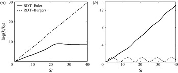The success of the SMC approach and its derivatives is dependent on the degree of predictive fidelity of the closure models for these individual terms. While physics-based closures for each of these terms are necessary, the pressure–strain correlation, embodying the action of pressure, is generally regarded as critically important (Sagaut & Cambon Reference Sagaut and Cambon2008). The rationale underlying this is twofold. The action of pressure is critically important in the evolution of turbulent flows. As an illustration depicted in figure 1, in different regimes of planar quadratic flows, the linear pressure effects either suppress (hyperbolic flow) or engender and sustain flow instabilities (elliptic flows). Thus, the pressure–strain correlation term determines if turbulence grows or decays in such flows and consequently, its accurate modelling is highly exigent. Additionally, the action of pressure is highly complex. The key issues that compound the complexity of turbulence are the inherent nonlinearity and non-locality. However, the ‘pressure-released’ Burgers turbulence, embodying much of the nonlinear character of turbulence, has been much better understood in contrast to its Navier–Stokes analogue (Cambon Reference Cambon1982; Sagaut & Cambon Reference Sagaut and Cambon2008). Consequently, the non-local action of pressure may be key toward understanding turbulent flows and their subsequent closure modelling.

Figure 1.

A contrast between the evolution exhibited in the Navier–Stokes system and the ‘pressure-released’ Burgers system, for the case of (a) a representative hyperbolic flow, (b) a representative elliptic flow.

In this context, various pressure–strain correlation models have been developed to date, such as those by Launder, Reece & Rodi (Reference Launder, Reece and Rodi1975), Speziale, Sarkar & Gatski (Reference Speziale, Sarkar and Gatski1991), Johansson & Hallback (Reference Johansson and Hallback1994), the structure-based model of Kassinos & Reynolds (Reference Kassinos and Reynolds1994), etc. However, the established closures still have some limitations in their robustness and scope. For instance, in rotation-dominated regimes like elliptic flows, while numerical simulations and linear stability exhibit flow instability, models may predict that the state of turbulence is decaying (Salhi, Cambon & Speziale Reference Salhi, Cambon and Speziale1997). Additionally, many investigators including Cambon & Rubinstein (Reference Cambon and Rubinstein2006) and Mishra & Girimaji (Reference Mishra and Girimaji2014) have exhibited that established models can ensure realizable Reynolds stress dynamics for low to moderate levels of anisotropy only. Consequently, their applicability to general turbulent flows is constrained. Thus, there exists a pressing need for a simple, robust and efficient closure for the pressure–strain correlation.

In the single-point closure approach, the classical modelling formulation attempts, via rational mechanics, to express the pressure–strain correlation as a function of local tensors, such as the Reynolds stresses, dissipation, the mean gradient tensor, etc. However, due to the assumption of incompressibility, pressure reacts instantaneously to any changes in the entire velocity field and is thus, a non-local variable. An attempt to develop single-point (or local) models for such non-local behaviour is inherently encumbered by a deficiency in required information. The set of local tensors do not constitute a complete basis to replicate the action of the pressure–strain correlation. This schism between the limitations of single-point statistics and the requirements mandated by physics forms the central problem in single-point modelling of the pressure–strain correlation.

Prior investigators have attempted to incorporate non-local effects into pressure–strain closures. For instance, in a spectral space description, the exact representation of the linear physics in flow evolution is enabled. This approach focuses on the spectral tensor $\hat{\unicode[STIX]{x1D619}}_{ij}$ , defined as the Fourier projection of the two-point second-order correlation, $\unicode[STIX]{x1D619}_{ij}(\boldsymbol{r},t)$ . Here, the nonlinear terms in the governing equation may be closed using the eddy-damped quasinormal Markovian (EDQNM) hypothesis. Such a procedure is utilized in Cambon, Jeandel & Mathieu (Reference Cambon, Jeandel and Mathieu1981) to derive a model for the $\unicode[STIX]{x1D705}$ -modulus spectrum of the rapid pressure–strain rate tensor in terms of the spherical integral of this spectral tensor. Another key hurdle in incorporating non-local dynamics is the inadequacy of the representation of turbulence anisotropy in terms of a single tensor. In terms of the $SO^{3}$ decomposition, the Reynolds stress anisotropy is represented as an infinite expansion in scalar and tensor spherical harmonics (Cambon & Rubinstein Reference Cambon and Rubinstein2006). At the lowest order of this expansion, weak anisotropy can be expressed in terms of two distinct tensors: directional and polarization anisotropy. In Cambon, Jacquin & Lubrano (Reference Cambon, Jacquin and Lubrano1992), a model is developed for the evolution of the directional and polarization anisotropies for solid-body mean rotation. This model is able to account for important phenomena, such as the damping of terms associated with nonlinear interactions at very low Rossby numbers and a nonlinear reorganization towards a two-dimensional state at intermediate Rossby numbers. Mons, Cambon & Sagaut (Reference Mons, Cambon and Sagaut2016) extend this methodology further. Herein, the directional-polarization decomposition is coupled with integration over spheres in Fourier space. This leads to expressions of the governing equations for the spherically averaged tensor depending only upon the wavevector modulus. Additionally, this spherical averaging approach enables a tractable and computationally reasonable final model. This model is not restricted to pure mean rotation, but is applicable to flows wherein mean gradient induced production effects are dominant in anisotropy evolution as opposed to the triple correlations. In physical space, Durbin (Reference Durbin1993) introduced a non-local model for the redistribution in strongly inhomogeneous flows. Here, the pressure–strain rate model is based on the solution of an elliptic relaxation equation, so as to be able to represent the inhomogeneity produced by the presence of walls. Due to its elliptic nature, the modelling of the redistribution due to the pressure–strain rate tensor is explicitly non-local.

The non-local nature of pressure is reflected in the fact that it is governed by a Poisson equation. In an incompressible turbulent flow, this is given by:

(1.2) $$\begin{eqnarray}\displaystyle \frac{1}{\unicode[STIX]{x1D70C}}\unicode[STIX]{x1D6FB}^{2}p=\underbrace{-2\frac{\unicode[STIX]{x2202}U_{i}}{\unicode[STIX]{x2202}x_{j}}\frac{\unicode[STIX]{x2202}u_{j}}{\unicode[STIX]{x2202}x_{i}}}_{\substack{ \text{Linear}\;\text{(rapid)} \\ \text{source}\;\text{term}}}\underbrace{-\frac{\unicode[STIX]{x2202}^{2}}{\unicode[STIX]{x2202}x_{i}\unicode[STIX]{x2202}x_{j}}(u_{i}u_{j}-\langle u_{i}u_{j}\rangle )}_{\substack{ \text{Nonlinear}\;\text{(slow)} \\ \text{source}\;\text{term}}}, & & \displaystyle\end{eqnarray}$$

wherein the lowercase symbols represent the fluctuating field, the mean fields are denoted by uppercase symbols and $\langle \cdot \rangle$ represents the ensemble averaging operator. With regard to the action of pressure, by precedent, fluctuating pressure is divided into two components, viz. rapid and slow pressure. Mathematically, the terms rapid and slow refer to the components of pressure arising from the linear and nonlinear parts of the source term, respectively. The slow component acts to conserve the incompressibility of the velocity field generated by the nonlinear interactions among velocity fluctuations. It is the function of rapid pressure to impose the divergence free condition on the fluctuating velocity field produced by the linear interactions between the mean and fluctuating fields. This action of rapid pressure (and consequently, the rapid pressure–strain correlation) has a complex dependence upon the mean velocity gradient and the state of the Reynolds stresses.

This investigation aims to address the modelling of the rapid pressure–strain correlation term. We outline a detailed methodology to formulate closures for the rapid pressure–strain correlation that possess reasonable agreement with physics and maintain adherence to the single-point modelling framework. To this end, the specific issues that are addressed include

1. (i) Compromises in the scope of the model: we discuss specific flow features, their importance in engineering prediction and their tractability to single-point closure modelling. Based on this analysis, we introduce a set of pragmatic compromises in the scope of the model.

2. (ii) Compromises in the structure of the model: the surrogates for non-local information in single-point closures are discussed and an approach to incorporate this information in a closure expression is presented.

3. (iii) Execution and analysis: as a proof of concept, we develop an illustrative model using this approach. The predictions of this model are compared to numerical and experimental data while being contrasted against other established models, for a range of different flows and flow conditions.

4. (iv) Applicability and extent: as a clear caveat emptor, we explicitly demarcate the zones of validity in Reynolds stress anisotropy space for this model, for different mean flows.

After an overview in § 1, we discuss the mathematical details of rapid pressure–strain correlation modelling in § 2. In § 3, the modelling methodology and the underlying rationale are outlined. Thereafter, as a proof of concept, we formulate an illustrative model adhering to this approach. In § 4, the predictions of this illustrative model are compared to numerical and experimental data, while being contrasted against other established closures. In § 5, using the process realizability constraints, the zones of validity of this illustrative model are identified for different mean flows. The article concludes with a summary of important findings and recommendations for future work, in § 6.

2 Mathematical background

At the rapid distortion limit, the turbulence-to-mean-shear time scale ratio is arbitrarily large. In the governing equations, the terms scaling with $S$ dominate, while the nonlinear terms become negligible in comparison (Moffatt Reference Moffatt1967b ). The consequent rapid distortion equations in physical space are given by:

(2.1a,b ) $$\begin{eqnarray}\displaystyle \frac{\bar{\text{D}}u_{j}}{\bar{\text{D}}t}=-u_{i}\frac{\unicode[STIX]{x2202}U_{j}}{\unicode[STIX]{x2202}x_{i}}-\frac{1}{\unicode[STIX]{x1D70C}}\frac{\unicode[STIX]{x2202}p^{(r)}}{\unicode[STIX]{x2202}x_{j}},\quad \frac{1}{\unicode[STIX]{x1D70C}}\unicode[STIX]{x1D6FB}^{2}p^{(r)}=-2\frac{\unicode[STIX]{x2202}U_{j}}{\unicode[STIX]{x2202}x_{i}}\frac{\unicode[STIX]{x2202}u_{i}}{\unicode[STIX]{x2202}x_{j}}, & & \displaystyle\end{eqnarray}$$

where $p^{(r)}$ refers to the rapid component of fluctuating pressure. These equations can be examined in Fourier space, via: $u_{i}(\boldsymbol{x},t)=\sum \hat{u} _{i}(\unicode[STIX]{x1D73F},t)\exp (\text{i}\unicode[STIX]{x1D73F}\boldsymbol{\cdot }\boldsymbol{x}),p^{(r)}(\boldsymbol{x},t)=\sum \hat{p}(\unicode[STIX]{x1D73F},t)\exp (\text{i}\unicode[STIX]{x1D73F}\boldsymbol{\cdot }\boldsymbol{x})$ . In Fourier space, the fluctuations are characterized in terms of the wavenumber vector, $\unicode[STIX]{x1D73F}(t)$ and $\hat{\boldsymbol{u}}$ , $\hat{p}$ , the corresponding modal Fourier amplitudes and pressure coefficients. As (2.1) are linear, each Fourier mode evolves independently and hence the equations can be decomposed and expressed for each mode separately. The modal evolution equations are (Moffatt Reference Moffatt1967a ):

(2.2a,b ) $$\begin{eqnarray}\displaystyle \frac{\text{d}\unicode[STIX]{x1D705}_{l}}{\text{d}t}=-\unicode[STIX]{x1D705}_{j}\frac{\unicode[STIX]{x2202}U_{j}}{\unicode[STIX]{x2202}x_{l}},\quad \frac{\text{d}\hat{u} _{j}}{\text{d}t}=-\hat{u} _{k}\frac{\unicode[STIX]{x2202}U_{l}}{\unicode[STIX]{x2202}x_{k}}\left(\unicode[STIX]{x1D6FF}_{jl}-2\frac{\unicode[STIX]{x1D705}_{j}\unicode[STIX]{x1D705}_{l}}{\unicode[STIX]{x1D705}^{2}}\right), & & \displaystyle\end{eqnarray}$$

and the incompressibility constraint is given by $\hat{\boldsymbol{u}}\boldsymbol{\cdot }\unicode[STIX]{x1D73F}=0$ . This indicates that the wavenumber vector and Fourier amplitude vector remain orthogonal. In the analysis, we utilize the unit wavenumber vector, $\boldsymbol{e}=\unicode[STIX]{x1D73F}/|\unicode[STIX]{x1D73F}|$ , as its phase space is compact and bounded.

In closure expressions, the rapid pressure–strain correlation (RPSC) is represented as a function of measurable tensors, using a general expression of the form $\unicode[STIX]{x03C0}_{ij}^{(r)}/k=\sum Q_{n}\unicode[STIX]{x1D61B}_{ij}^{n}$ , wherein $\unicode[STIX]{x1D61B}_{ij}^{n}$ are symmetric, deviatoric tensors and $Q_{n}$ are the corresponding model coefficients. The most general form of such a RPSC expression is (Johansson & Hallback Reference Johansson and Hallback1994)

(2.3) $$\begin{eqnarray}\displaystyle \frac{\unicode[STIX]{x03C0}_{ij}^{(r)}}{k} & = & \displaystyle S_{pq}\left(Q_{1}\unicode[STIX]{x1D6FF}_{ip}\unicode[STIX]{x1D6FF}_{jq}+Q_{2}\left(b_{ip}\unicode[STIX]{x1D6FF}_{jq}+\unicode[STIX]{x1D6FF}_{iq}b_{jp}-\frac{2}{3}b_{pq}\unicode[STIX]{x1D6FF}_{ij}\right)\right.\nonumber\\ \displaystyle & & \displaystyle +\,Q_{3}b_{pq}\unicode[STIX]{x1D623}_{ij}+Q_{4}\left(b_{iq}b_{jp}-\frac{1}{3}b_{pk}b_{qk}\unicode[STIX]{x1D6FF}_{ij}\right)+Q_{5}b_{pl}b_{ql}\unicode[STIX]{x1D623}_{ij}\nonumber\\ \displaystyle & & \displaystyle +\,\left.(Q_{5}b_{pq}+Q_{6}b_{pl}b_{ql})\left(b_{ik}b_{jk}-\frac{1}{3}II_{a}\unicode[STIX]{x1D6FF}_{ij}\right)\right)\nonumber\\ \displaystyle & & \displaystyle +\,W_{pq}(Q_{7}(b_{ip}\unicode[STIX]{x1D6FF}_{jq}+b_{jp}\unicode[STIX]{x1D6FF}_{iq})+Q_{8}b_{pk}(b_{jk}\unicode[STIX]{x1D6FF}_{iq}+b_{ik}\unicode[STIX]{x1D6FF}_{jq})+Q_{9}b_{pk}(b_{jk}b_{iq}+b_{ik}b_{jq})).\qquad\end{eqnarray}$$

Here, $\unicode[STIX]{x1D61E}_{ij}$ and $\unicode[STIX]{x1D61A}_{ij}$ refer to the rate of rotation and rate of strain tensors of the mean flow, $\unicode[STIX]{x1D623}_{ij}=\overline{u_{i}u_{j}/2k}-\unicode[STIX]{x1D70E}_{ij}/3$ denotes the Reynolds stress anisotropy and $k$ , the turbulent kinetic energy. The modelling of the rapid pressure–strain correlation is tantamount to modelling the forth-order $\unicode[STIX]{x1D614}_{ijkl}$ tensor. Explicitly, the relationship is given by (Johansson & Hallback Reference Johansson and Hallback1994)

(2.4) $$\begin{eqnarray}\displaystyle \unicode[STIX]{x03C0}_{ij}^{(r)}=4k\frac{\unicode[STIX]{x2202}U_{l}}{\unicode[STIX]{x2202}x_{k}}(\unicode[STIX]{x1D614}_{kjil}+\unicode[STIX]{x1D614}_{ikjl}),\quad \text{wherein},\unicode[STIX]{x1D614}_{ijpq}=-\frac{1}{8\unicode[STIX]{x03C0}k}\int \frac{1}{|\boldsymbol{r}|}\frac{\unicode[STIX]{x2202}^{2}\unicode[STIX]{x1D619}_{ij}(\boldsymbol{r})}{\unicode[STIX]{x2202}r_{p}\unicode[STIX]{x2202}r_{q}}\,\text{d}\boldsymbol{r}, & & \displaystyle\end{eqnarray}$$

where $\unicode[STIX]{x1D619}_{ij}(\boldsymbol{r})=\langle u_{i}(\boldsymbol{x})u_{j}(\boldsymbol{x}+\boldsymbol{r})\rangle$ , is the two-point velocity correlation. It is expedient to model this fourth-order tensor, as the constraints on the $\unicode[STIX]{x1D648}$ tensor expression are more comprehensive. The most general expression for $\unicode[STIX]{x1D648}$ is (Johansson & Hallback Reference Johansson and Hallback1994):

(2.5) $$\begin{eqnarray}\displaystyle \unicode[STIX]{x1D614}_{ijpq} & = & \displaystyle A_{1}\unicode[STIX]{x1D6FF}_{ij}\unicode[STIX]{x1D6FF}_{pq}+A_{2}(\unicode[STIX]{x1D6FF}_{ip}\unicode[STIX]{x1D6FF}_{jq}+\unicode[STIX]{x1D6FF}_{iq}\unicode[STIX]{x1D6FF}_{jp})+A_{3}\unicode[STIX]{x1D6FF}_{ij}b_{pq}+A_{4}\unicode[STIX]{x1D6FF}_{pq}\unicode[STIX]{x1D623}_{ij}\nonumber\\ \displaystyle & & \displaystyle +\,A_{5}(\unicode[STIX]{x1D6FF}_{ip}b_{jq}+\unicode[STIX]{x1D6FF}_{iq}b_{jp}+\unicode[STIX]{x1D6FF}_{jp}b_{iq}+\unicode[STIX]{x1D6FF}_{jq}b_{ip})+A_{6}\unicode[STIX]{x1D623}_{ij}b_{pq}+A_{7}(b_{ip}b_{jq}+b_{iq}b_{jp})+A_{8}b_{pk}b_{qk}\unicode[STIX]{x1D6FF}_{ij}\nonumber\\ \displaystyle & & \displaystyle +\,A_{9}b_{ik}b_{jk}\unicode[STIX]{x1D6FF}_{pq}+A_{10}(b_{ik}b_{pk}\unicode[STIX]{x1D6FF}_{jq}+b_{jk}b_{pk}\unicode[STIX]{x1D6FF}_{iq}+b_{ik}b_{qk}\unicode[STIX]{x1D6FF}_{jp}+b_{jk}b_{qk}\unicode[STIX]{x1D6FF}_{ip})\nonumber\\ \displaystyle & & \displaystyle +\,A_{11}\unicode[STIX]{x1D623}_{ij}b_{pk}b_{qk}+A_{12}b_{pq}b_{ik}b_{jk}+A_{13}(b_{ik}b_{pk}b_{jq}+b_{jk}b_{pk}b_{iq}+b_{ik}b_{qk}b_{jp}+b_{jk}b_{qk}b_{ip})\nonumber\\ \displaystyle & & \displaystyle +\,A_{14}b_{ik}b_{jk}b_{pl}b_{ql}+A_{15}b_{ik}b_{jl}(b_{pk}b_{ql}+b_{qk}b_{pl}).\end{eqnarray}$$

The constraints on the closure expression for the $\unicode[STIX]{x1D648}$ tensor are (Johansson & Hallback Reference Johansson and Hallback1994):

1. (i) symmetry conditions, with respect to the indices ( $\unicode[STIX]{x1D614}_{ijkl}=\unicode[STIX]{x1D614}_{jikl},\unicode[STIX]{x1D614}_{ijkl}=\unicode[STIX]{x1D614}_{ijlk}$ );

2. (ii) continuity condition ( $\unicode[STIX]{x1D614}_{ijil}=0$ );

3. (iii) Green’s condition ( $\unicode[STIX]{x1D614}_{ijkk}=\unicode[STIX]{x1D619}_{ij}/2k$ );

4. (iv) for isotropic turbulence, $\unicode[STIX]{x1D614}_{ijkl}=1/30(4\unicode[STIX]{x1D70E}_{ij}\unicode[STIX]{x1D70E}_{kl}-\unicode[STIX]{x1D70E}_{ik}\unicode[STIX]{x1D70E}_{jl}-\unicode[STIX]{x1D70E}_{il}\unicode[STIX]{x1D70E}_{jk})$ .

The pressure–strain correlation engendered by such an $\unicode[STIX]{x1D648}$ tensor expression should lead to a high degree to predictive fidelity, as well as adherence to realizability (Schumann Reference Schumann1977; du Vachat Reference du Vachat1977; Lumley Reference Lumley1978). As has been observed in literature, these properties pertain to an ideal model and at present, no model can conform to all these requirements due to the inherent limitation of the single-point modelling framework. Thus, the exercise of modelling seeks to develop a ‘best-possible’ model, while adhering to important guidelines.

Figure 2.

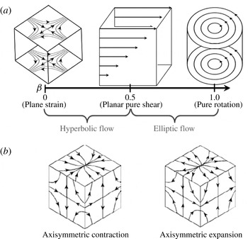
Flow regimes considered (a) quadratic flows and their classification, (b) non-planar axisymmetric flows.

In this article, we consider the canonical set of flows termed quadratic flows (Salhi et al. Reference Salhi, Cambon and Speziale1997), including benchmark cases such as plane strain, purely sheared and purely rotating flows. To characterize the mean gradient, we introduce the ellipticity parameter, $\unicode[STIX]{x1D6FD}$ , defined as (Mishra et al. Reference Mishra, Hasan, Sanghi and Kumar2008; Mishra & Girimaji Reference Mishra and Girimaji2013, Reference Mishra and Girimaji2015): $\unicode[STIX]{x1D6FD}=(W_{pq}W_{pq}/\unicode[STIX]{x1D61E}_{ij}\unicode[STIX]{x1D61E}_{ij}+\unicode[STIX]{x1D61A}_{ij}\unicode[STIX]{x1D61A}_{ij})$ . Planar quadratic flows can be uniquely characterized by the value of $\unicode[STIX]{x1D6FD}$ , as exhibited in figure 2(a). In addition to this family of flows, we consider the non-planar cases of axisymmetric expansion and contraction. For comparisons with DNS and experiments, we utilize the modelled evolution equation for dissipation given by

(2.6) $$\begin{eqnarray}\displaystyle \frac{\text{d}\unicode[STIX]{x1D716}}{\text{d}t}=C_{\unicode[STIX]{x1D716}1}\frac{\unicode[STIX]{x1D716}}{k}P-C_{\unicode[STIX]{x1D716}2}\frac{\unicode[STIX]{x1D716}^{2}}{k}, & & \displaystyle\end{eqnarray}$$

with $C_{\unicode[STIX]{x1D716}1}=1.44$ and $C_{\unicode[STIX]{x1D716}2}=1.88$ . Additionally, for the slow pressure–strain correlation, we utilize the linear model of Rotta (Reference Rotta1951) of the form:

(2.7) $$\begin{eqnarray}\displaystyle \dot{\unicode[STIX]{x1D623}}_{ij}=\frac{\unicode[STIX]{x1D716}}{k}(1-C_{R})\unicode[STIX]{x1D623}_{ij}, & & \displaystyle\end{eqnarray}$$

where $C_{R}=1.5$ is Rotta’s constant.

3 Modelling methodology

According to theoretical guidelines, at the rapid distortion limit the functional dependence of the pressure–strain correlation is of the form:

(3.1) $$\begin{eqnarray}\displaystyle \unicode[STIX]{x03C0}_{ij}^{RDT}=\unicode[STIX]{x03C0}(\unicode[STIX]{x1D61A}_{ij},\unicode[STIX]{x1D61E}_{ij},e_{i}e_{j}\hat{u} _{k}\hat{u} _{l}). & & \displaystyle\end{eqnarray}$$

However, due to the non-local nature of wavevector information, in single-point closures as a compromise, $\unicode[STIX]{x03C0}_{ij}$ is modelled in terms of local tensors:

(3.2) $$\begin{eqnarray}\displaystyle \unicode[STIX]{x03C0}_{ij}^{model}=\unicode[STIX]{x03C0}(\unicode[STIX]{x1D61A}_{ij},\unicode[STIX]{x1D61E}_{ij},\unicode[STIX]{x1D619}_{ij}). & & \displaystyle\end{eqnarray}$$

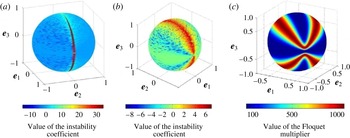
This substitution (of $e_{i}e_{j}\hat{u} _{k}\hat{u} _{l}$ by $\unicode[STIX]{x1D619}_{ij}$ ) limits the modelling framework as the wavevector space information is cardinal to important flow features. For instance, the faithful representation of the instabilities in hyperbolic, purely sheared and elliptic flows requires wavevector space information. In these flows, only small sets of modes show any degree of unstable behaviour. The stability and evolution of the modes are completely dependent upon their alignment with respect to the applied mean gradient, exhibited in figure 3. Furthermore, while transitioning from hyperbolic to elliptic flows, the governing equations undergo a saddle-node bifurcation and the nature of the solutions changes. While flow statistics evolve to stationary states for hyperbolic flows, in elliptic flows they exhibit oscillatory behaviour. However, this bifurcation is manifested in the wavevector evolution equation and its replication requires non-local information. Similarly, in elliptic flows, the flow statistics exhibit bilinear oscillations (Mishra & Girimaji Reference Mishra and Girimaji2010, Reference Mishra and Girimaji2012). The nature of the oscillations is governed by the dynamics of the wavevector and is not available in any local basis. With such limitations in mind, we introduce a set of pragmatic compromises within the form and the scope of the model, so as to develop models having an augmented degree of agreement with physics while still maintaining adherence to the single-point modelling framework.

Figure 3.

Topology of the unstable modes in spectral space for an open streamline flow, a purely sheared flow and a closed streamline flow. Such a schematic representation was initiated by Cambon et al. (Reference Cambon, Benoit, Shao and Jacquin1994).

3.1 Nature of the modelling expression

We recommend that the expression for the rapid pressure–strain correlation be a linear function of the Reynolds stress anisotropies. The rationale underlying this is threefold. Firstly, the Poisson equation governing rapid pressure is linear in the fluctuating velocities. Consequently, the ideal rapid pressure–strain correlation closure should conserve the number of Fourier modes in the representation of the fluctuating field. This would require closure expressions that are linear in the Reynolds stresses.

The inability of such linear models to comply with state realizability is one of the principal arguments in favour of nonlinear closure expressions. However, models with complex nonlinear expressions may exhibit unphysical behaviour, such as spurious oscillations in the vicinity of the two-component (2C) state (Speziale, Abid & Durbin Reference Speziale, Abid and Durbin1994). Further, Mishra & Girimaji (Reference Mishra and Girimaji2014) have exhibited that nonlinear closure expressions may not yield a better representation of the Reynolds stress dynamics.

Finally, closure expressions linear in the Reynolds stresses are advantageous as they lead to simpler application in the derivation of corresponding algebraic Reynolds stress models and Langevin equation-based stochastic models (Speziale & Durbin Reference Speziale and Durbin1994). With this simplification, the model expression (2.3) reduces to

(3.3) $$\begin{eqnarray}\displaystyle \frac{\unicode[STIX]{x03C0}_{ij}^{(r)}}{k}=S_{pq}\left(Q_{1}\unicode[STIX]{x1D6FF}_{ip}\unicode[STIX]{x1D6FF}_{jq}+Q_{2}\left(b_{ip}\unicode[STIX]{x1D6FF}_{jq}+\unicode[STIX]{x1D6FF}_{iq}b_{jp}-\frac{2}{3}b_{pq}\unicode[STIX]{x1D6FF}_{ij}\right)\right)+W_{pq}(Q_{7}(b_{ip}\unicode[STIX]{x1D6FF}_{jq}+b_{jp}\unicode[STIX]{x1D6FF}_{iq})).\quad & & \displaystyle\end{eqnarray}$$

3.2 Nature of the model coefficients

Figure 4.

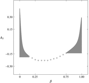
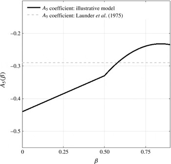
Permissible ranges for the $A_{5}$ coefficient with respect to the ellipticity parameter, $\unicode[STIX]{x1D6FD}$ , as determined by the process realizability constraints.

Herein, the mean velocity gradient may be a partial substitute for certain features of the missing wavespace information. This is contingent upon three reasons:

1. (a) Universal evolution of modal trajectories dependent on mean gradient: Mishra & Girimaji (Reference Mishra and Girimaji2013) have shown that in homogeneous flows, due to the invariant sets in the phase space, the wavenumber vector trajectories exhibit universal dynamics. After a very brief transient, almost all unstable sets of modes in wavenumber vector space exhibit similar behaviour that can be characterized via the mean velocity gradient invariants. Thus, inclusion of the mean velocity gradient invariants into the basis for the $\unicode[STIX]{x1D648}$ tensor, may lead to better fidelity of predictions.

   The closure coefficients in a single-point model have explicit dependence on the wavevector space information and presuppose a value for the dimensionality of the flow, explicitly, $Q_{i}^{ideal}=Q_{i}(\boldsymbol{e},II_{b},III_{b})$ , where $II_{b},III_{b}$ are the invariants of the Reynolds stress anisotropy. Considering the evolution of the unit wavenumber vectors in the ensemble $\boldsymbol{e}(t)=\boldsymbol{e}(\unicode[STIX]{x1D6FD},\boldsymbol{e}(0))$ , we recommend a compromise, wherein $Q_{i}^{model}=Q_{i}(\unicode[STIX]{x1D6FD},II_{b},III_{b})$ .

2. (b) Dependence of realizability constraints on the mean gradient: the process realizability framework focuses on the realizability of Reynolds stress dynamics and applies constraints upon the closure expression for the $\unicode[STIX]{x1D648}$ tensor. These constraints are explicit functions of the mean velocity gradient. Consequently, to ensure the physical permissibility of the Reynolds stresses, the coefficients of the $\unicode[STIX]{x1D648}$ tensor expression must be explicit functions of the mean velocity gradient, as is exhibited in figure 4. The figure underscores the need for modification of the coefficients with changes in the mean velocity gradient. In summary, using the mean gradient information in the expression for the $\unicode[STIX]{x1D648}$ tensor may enable better of replication of Reynolds stress dynamics.

3. (c) Extensibility of such a framework: it has been shown (Mishra, Iaccarino & Duraisamy Reference Mishra, Iaccarino and Duraisamy2015, Reference Mishra, Iaccarino and Duraisamy2016) that the uncertainty in the predictions of turbulence models is highly dependent on the mean gradient. The mean of flow statistics over different modal ensembles and the associated prediction intervals are explicit functions of the invariants of the mean velocity gradient. Models for the $\unicode[STIX]{x1D648}$ tensor incorporating the mean gradient information in the coefficients are highly amenable to such Bayesian approaches.

In summation, the fundamental shortcomings in single-point turbulence models lie in their predictive fidelity, the realizability violations and the epistemic uncertainty in predictions. However, in prior investigations, it has been shown that each of these deficiencies are strong functions of the mean velocity gradient. In this light, the mean velocity gradient may represent a surrogate for the wavevector space information. With this rationale, the model expression reduces to

(3.4) $$\begin{eqnarray}\displaystyle \frac{\unicode[STIX]{x03C0}_{ij}^{(r)}}{k} & = & \displaystyle S_{pq}\left(Q_{1}(\unicode[STIX]{x1D6FD})\unicode[STIX]{x1D6FF}_{ip}\unicode[STIX]{x1D6FF}_{jq}+Q_{2}(\unicode[STIX]{x1D6FD})\left(b_{ip}\unicode[STIX]{x1D6FF}_{jq}+\unicode[STIX]{x1D6FF}_{iq}b_{jp}-\frac{2}{3}b_{pq}\unicode[STIX]{x1D6FF}_{ij}\right)\right)\nonumber\\ \displaystyle & & \displaystyle +\,W_{pq}(Q_{7}(\unicode[STIX]{x1D6FD})(b_{ip}\unicode[STIX]{x1D6FF}_{jq}+b_{jp}\unicode[STIX]{x1D6FF}_{iq})).\end{eqnarray}$$

Figure 5.

Compromise in the scope of the modelling objective: the relative importance of the oscillatory dynamics.

Applying the consistency conditions on the $\unicode[STIX]{x1D648}$ tensor, this expression can be simplified and the set of coefficients $(Q_{1},Q_{2},Q_{7})$ can be expressed in terms of a single parameter. We utilize the $A_{5}$ coefficient from (2.5), reducing the expression to:

(3.5) $$\begin{eqnarray}\displaystyle \frac{\unicode[STIX]{x03C0}_{ij}^{(r)}}{k} & = & \displaystyle \frac{4}{5}\unicode[STIX]{x1D61A}_{ij}-6A_{5}(\unicode[STIX]{x1D6FD})S_{pq}\left(b_{ip}\unicode[STIX]{x1D6FF}_{jq}+b_{jp}\unicode[STIX]{x1D6FF}_{iq}+\frac{2}{3}b_{pq}\unicode[STIX]{x1D6FF}_{ij}\right)\nonumber\\ \displaystyle & & \displaystyle +\,\frac{2}{3}(4+7A_{5}(\unicode[STIX]{x1D6FD}))W_{pq}(b_{ip}\unicode[STIX]{x1D6FF}_{jq}+b_{jp}\unicode[STIX]{x1D6FF}_{iq}).\end{eqnarray}$$

3.3 Scope of the model

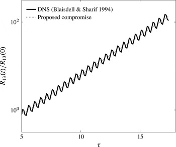
From an engineering perspective, the dynamics of the oscillatory behaviour in elliptic flows is relatively unimportant as compared to the evolution of the mean of the flow statistics. As an illustration, we consider the DNS results of Blaisdell & Shariff (Reference Blaisdell and Shariff1996) in figure 5. As is schematically exhibited, a model that is able to replicate the evolution of the mean while ignoring the oscillations, may be of significant engineering utility. Additionally, adopting such a simplification precludes the necessity of considering the bifurcations in the system, as for either variety of flow (strain or rotation dominated), the model aims to predict stationary states.

With these compromises in the form and the scope of the model, the functional relationship of the coefficient $A_{5}$ on the mean gradient field needs to be determined. For the purposes of an illustration, we use simulations at the rapid distortion limit to ascertain this. We utilize an ensemble of wavevectors corresponding to an isotropic initial state, where the Fourier coefficients of initial velocity fluctuations in all directions have equal magnitudes. Herein, the system’s dynamics is not biased in any manner and the unstable modes are able to dominate the flow statistics accordingly. This leads to the statistically most likely (SML) behaviour identified in prior investigations (Mishra & Girimaji Reference Mishra and Girimaji2013). After the initial transient, we average the individual $e_{i}(t)e_{j}(t)\hat{u} _{k}(\unicode[STIX]{x1D705},t)\hat{u} _{l}(\unicode[STIX]{x1D705},t)$ to get the value of the $A_{5}$ coefficient that gives the least mean square error. This leads to a curve determining the value of the coefficient $A_{5}$ with respect to the ellipticity parameter, $\unicode[STIX]{x1D6FD}$ , as exhibited in figure 6. The variation of the $A_{5}$ coefficient of the illustrative model is given by:

(3.6) $$\begin{eqnarray}\displaystyle \left.\begin{array}{@{}c@{}}A_{5}(\unicode[STIX]{x1D6FD})=0.22\times \unicode[STIX]{x1D6FD}-0.44,\unicode[STIX]{x1D6FD}\in [0,0.5]\\ A_{5}(\unicode[STIX]{x1D6FD})=-0.83\times \unicode[STIX]{x1D6FD}^{2}+1.4\times \unicode[STIX]{x1D6FD}-0.82,\unicode[STIX]{x1D6FD}\in (0.5,1).\end{array}\right\} & & \displaystyle\end{eqnarray}$$

Figure 6.

The functional relationship between $A_{5}$ and the ellipticity parameter, $\unicode[STIX]{x1D6FD}$ .

4 Fidelity of the illustrative model

In this section, the predictions of this illustrative model are compared to numerical and experimental data while being contrasted against established closures. These closures represent different modelling approaches, with respect to their adherence to the constraints imposed upon an ideal model. The model of Launder et al. (Reference Launder, Reece and Rodi1975) adheres to all the constraints. Using an invariant dynamics approach, the model of Speziale et al. (Reference Speziale, Sarkar and Gatski1991) utilizes a closure expression that is quadratic in the components of the Reynolds stress tensor and the coefficients used therein are scalar functions of the invariants of the Reynolds stress anisotropy tensor. This allows the closure to adhere to a weak form of the realizability condition and exhibit better predictions, especially for purely sheared flows. The closure of Johansson & Hallback (Reference Johansson and Hallback1994) utilizes fourth-order expansions in the components of the Reynolds stress anisotropy tensor. This enables the model to satisfy the strong form of the realizability constraint for all states of the anisotropy invariant map and exhibit improved agreement with experimental data. The model of Kassinos & Reynolds (Reference Kassinos and Reynolds1994) (specifically, the linear $M(b,y,Q^{\ast })$ model formulated in § 3 of the reference) attempts to append additional tensors in the modelling basis, such as dimensionality, $\unicode[STIX]{x1D60B}_{ij}$ , circulicity, $\unicode[STIX]{x1D60D}_{ij}$ and stropholysis, $\unicode[STIX]{x1D618}_{ijk}$ . For homogeneous turbulence, these can be defined as: $\unicode[STIX]{x1D619}_{ij}=\unicode[STIX]{x1D614}_{ijkk},\unicode[STIX]{x1D60B}_{ij}=\unicode[STIX]{x1D614}_{kkij},\unicode[STIX]{x1D60D}_{ij}=\unicode[STIX]{x1D716}_{imp}\unicode[STIX]{x1D716}_{jrs}\unicode[STIX]{x1D614}_{psrm},\unicode[STIX]{x1D618}_{ijk}=\unicode[STIX]{x1D716}_{ipq}\unicode[STIX]{x1D614}_{jqpk}$ . Kassinos & Reynolds (Reference Kassinos and Reynolds1994) have concluded that while this $M(b,y,Q^{\ast })$ model is able to exhibit some improvement as compared to classical closures, it still has certain limitations in rotation-dominated flows.

Table 1.

The set of flows utilized and the rationale thereof.

In the interest of brevity, we outline only a few cases for this comparison in this article. A detailed analysis with additional cases and additional flow statistics is contained in Mishra (Reference Mishra2014, Reference Mishra2010). The flows utilized in this article are discussed in table 1, along with the rationale underlying the choice. The objective of this section is to exhibit that the illustrative model developed in the last section is able to exhibit predictions that are comparable with other models for the regimes of flow wherein established models perform adequately. In regimes where established models may not exhibit satisfactory performance, the illustrative model is still able to provide predictions of engineering utility.

4.1 Performance for hyperbolic flows

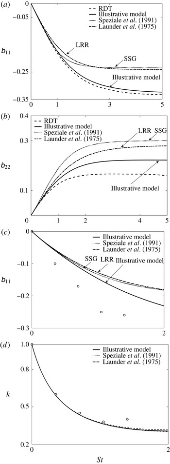
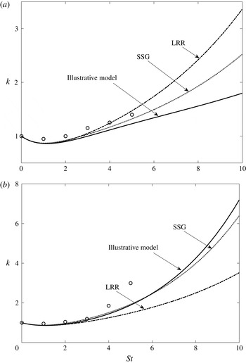
In figure 7, the predictions of the illustrative model are compared to DNS data and contrasted against other popular models for the case of a plane strain mean flow. Owing to the low Reynolds number in the DNS of Lee & Reynolds (Reference Lee and Reynolds1985), we append additional hyperbolic flows in the rapid distortion limit to the test cases. As can be observed, the illustrative model is able to ensure satisfactory agreement with numerical data.

Figure 7.

Fidelity for hyperbolic flows: (a,b) anisotropy evolution for plane strain in the rapid distortion limit; (c,d) anisotropy and turbulent kinetic evolution for plane strain with $\unicode[STIX]{x1D716}_{0}/Sk_{0}=2$ . The circles mark the DNS of Lee & Reynolds (Reference Lee and Reynolds1985).

Figure 8.

Fidelity for axisymmetric contraction: the circles mark the DNS of Lee & Reynolds (Reference Lee and Reynolds1985), for $\unicode[STIX]{x1D716}_{0}/Sk_{0}=0.179$ .

Figure 9.

Fidelity for the case of a purely sheared flow, with and without rotation of the coordinate axes. The circles mark the large-eddy simulation (LES) of Bardina, Ferziger & Reynolds (Reference Bardina, Ferziger and Reynolds1983), for $\unicode[STIX]{x1D716}_{0}/Sk_{0}=0.296$ . (a) $\unicode[STIX]{x1D714}/S=0.0$ , (b) $\unicode[STIX]{x1D714}/S=0.25$ .

4.3 Performance for the case of rotating shear

In figure 9, the predictions of the illustrative model are compared to DNS data and contrasted against other established models for the case of a shear flow with and without rotation of the coordinate axes. This family of flows is important as the second moment closures need to account for both the incipient instability of the purely sheared flow, as well as the effect of the rotation of the coordinate axes on the instability. As can be observed, the illustrative model is able to ensure good agreement with LES results.

Figure 10.

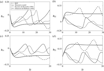
Fidelity under the rapid distortion assumption: (a,b) elliptic flow with $\unicode[STIX]{x1D6FD}=0.55$ ; (c,d) elliptic flow with $\unicode[STIX]{x1D6FD}=0.65$ .

4.5 Performance for elliptic flows

Figure 11.

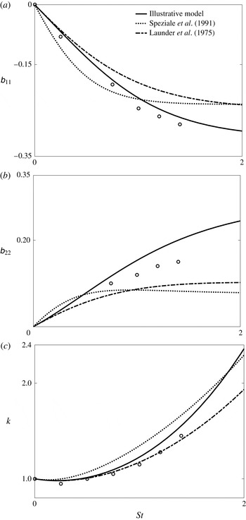
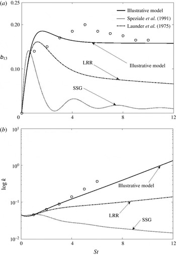
Fidelity for the case of an elliptic flow with $\unicode[STIX]{x1D6FD}=0.74$ . The circles mark the DNS of Blaisdell & Shariff (Reference Blaisdell and Shariff1996). (a) Anisotropy evolution, (b) turbulent kinetic evolution.

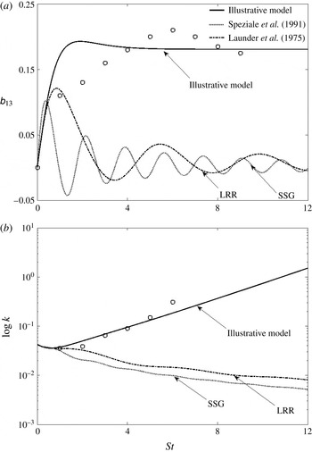
In figure 11, the predictions of the illustrative model are compared to the DNS data of Blaisdell & Shariff (Reference Blaisdell and Shariff1996) and contrasted against other established closures for the case of an elliptic mean flow ( $\unicode[STIX]{x1D6FD}=0.74$ ). As can be observed, the new modelling approach is able to give significant agreement for the anisotropy evolution. For the evolution of the turbulent kinetic energy, under the influence of the elliptic flow instability, the illustrative model is able to capture both the existence of unstable behaviour, as well as the growth rate. As the ellipticity parameter is increased, the predictions of established models are exacerbated, as is reflected in figure 12. Herein, while DNS simulations suggest that the flow is unstable, the models of Launder et al. (Reference Launder, Reece and Rodi1975) and Speziale et al. (Reference Speziale, Sarkar and Gatski1991) predict that turbulence is decaying. However, even for such high values of $\unicode[STIX]{x1D6FD}$ , the illustrative model is able to predict the evolution of flow statistics with reasonable fidelity.

Figure 12.

Fidelity for the case of an elliptic flow with $\unicode[STIX]{x1D6FD}=0.87$ . The circles mark the DNS of Blaisdell & Shariff (Reference Blaisdell and Shariff1996). (a) Anisotropy evolution, (b) turbulent kinetic evolution.

5 Model applicability: realizability of the Reynolds stress dynamics

The incomplete basis used in pressure–strain correlation modelling leads to the inapplicability of second moment closures at higher values of anisotropy (Cambon & Rubinstein Reference Cambon and Rubinstein2006; Sagaut & Cambon Reference Sagaut and Cambon2008). In the investigation of Mishra & Girimaji (Reference Mishra and Girimaji2014), it is shown that some established models can ensure realizable predictions only for low to moderate levels of anisotropy. All models have significantly large regions on the anisotropy invariant map wherein they are unable to ensure realizable Reynolds stress dynamics. For this modelling approach, we suggest that the process realizability constraints developed in Mishra & Girimaji (Reference Mishra and Girimaji2014) be applied, to unequivocally demarcate the states of turbulence wherein the model is able to ensure realizability for specific mean flows. Such explicit delineation of the extent of the validity of the closure acts as a caveat emptor in the process of its application to engineering problems.

Figure 13.

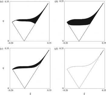
Process realizability adherence of the illustrative model for quadratic flows, $\unicode[STIX]{x1D6FD}=0$ , 0.5, 0.75 and 1.

For the explicit procedure of this demarcation, the reader is referred to Mishra & Girimaji (Reference Mishra and Girimaji2014). Herein, we apply the set of process realizability constraints to exhibit the zones of validity of the illustrative model for different planar quadratic mean flows, as exhibited in figure 13. The regions of the anisotropy invariant map wherein the illustrative model is unable to ensure permissible Reynolds stress dynamics are shaded. In line with the limitation discussed earlier, the illustrative model is unable to ensure realizable Reynolds stress dynamics in a small neighbourhood of the 2C limit. For elliptic flows, the illustrative model is able to ensure realizable dynamics for larger regions of the anisotropy invariant map. In the limit of purely rotating flow, only a small neighbourhood of the one-component (1C) limit remains unrealizable. It must be emphasized that for the case of hyperbolic and purely sheared flows, the model shows process realizability adherence that is comparable to other closures such as those of Launder et al. (Reference Launder, Reece and Rodi1975) and Speziale et al. (Reference Speziale, Sarkar and Gatski1991). For the case of elliptic flows, the illustrative model shows process realizability adherence that is significantly better than established models (Mishra & Girimaji Reference Mishra and Girimaji2014).

6 Summary and conclusions

In this investigation, we identify important challenges in the modelling of turbulence physics and outline a framework to formulate pressure–strain correlation models that possess augmented agreement with linear physics while still adhering to the single-point closure formalism. We discuss specific flow features, their importance in engineering prediction and their tractability to single-point closure modelling. Based on this analysis, we suggest a set of pragmatic compromises with respect to the scope of the turbulent statistics to be modelled and the form of the closure. Thence, this methodology is utilized to formulate an illustrative model. The predictions of this model are compared to numerical and experimental data while being contrasted against other popular modelling approaches for a wide range of homogeneous turbulent flows under diverse conditions. This illustrative model is able to exhibit predictions that are comparable to other closures for the regimes of flow wherein these established models perform adequately. Moreover, in regimes wherein established models may not exhibit satisfactory performance, the illustrative model is still able to provide predictions of engineering utility. Finally, the zones of validity of this model are delineated for different mean flows.

Using a mean gradient invariant as a surrogate for the wavenumber space information may have the additional benefit of allowing this modelling methodology to be extended to general three-dimensional homogeneous turbulent flows. This line of inquiry is being pursued. Additionally, due to the incomplete basis, there is an inherent degree of uncertainty associated with the predictions of a single-point closure model. We are in the process of quantifying the requisite prediction intervals contingent upon this modelling methodology.