1 Introduction
The motion of an elastic interface near a solid substrate manifests itself in microelectronic engineering processes (Chaudhury & Pocius Reference Chaudhury and Pocius2002; Longley, Mahadevan & Chaudhury Reference Longley, Mahadevan and Chaudhury2013), membrane adhesives (Hosoi & Mahadevan Reference Hosoi and Mahadevan2004; Leong & Chiam Reference Leong and Chiam2010), synthetic lipid membrane systems (Cantat & Misbah Reference Cantat and Misbah1998; Reister-Gottfried et al. Reference Reister-Gottfried, Sengupta, Lorz, Sackmann, Seifert and Smith2008), geology (Michaut Reference Michaut2011; Lister, Peng & Neufeld Reference Lister, Peng and Neufeld2013; Nesic et al. Reference Nesic, Cuerno, Moro and Kondic2015a ), as well as in a myriad of biological processes including adhesion of epithelial cell sheets, bio-films (Wilking et al. Reference Wilking, Zaburdaev, De Volder, Losick, Brenner and Weitz2013), membrane blebbing (Alert & Casademunt Reference Alert and Casademunt2016) and cell adhesion (Bell Reference Bell1984; Bongrand Reference Bongrand1998). The spatio-temporal dynamics of these interfaces is composed of the complex interplay between the deterministic forces associated with the interface dynamics i.e. viscous film flow, membrane bending and tension, and stochastic effects from the environment.
Coarse-grained models and the inclusion of stochastic stress terms into a continuum formulation are alternative approaches to a molecular description (Garcia-Ojalvo, Hernandez-Machado & Sancho Reference Garcia-Ojalvo, Hernandez-Machado and Sancho1993; Moseler & Landman Reference Moseler and Landman2000; Grün, Mecke & Rauscher Reference Grün, Mecke and Rauscher2006; Johansson, Carlson & Hess Reference Johansson, Carlson and Hess2015; Diez, Gonzalez & Fernandez Reference Diez, Gonzalez and Fernandez2016) to describe the interface dynamics. The development of phenomenological hydrodynamic models with a thermal noise term have a long history dating back to the seminal work by Landau & Lifshitz (Reference Landau and Lifshitz1959) and Fox & Uhlenbeck (Reference Fox and Uhlenbeck1970). Dynamics of capillary flows e.g. breakup of a liquid tread (Moseler & Landman Reference Moseler and Landman2000), rupture and de-wetting of thin liquid films (Herminghaus, Jacobs & Seemann Reference Herminghaus, Jacobs and Seemann2001; Seemann, Herminghaus & Jacobs Reference Seemann, Herminghaus and Jacobs2001; Felzer et al.
Reference Fetzer, Rauscher, Seemann, Jacobs and Mecke2007), drop spreading (Davidovitch, Moro & Stone Reference Davidovitch, Moro and Stone2005) and contact angle dynamics (Belardinelli et al.
Reference Belardinelli, Sbragaglia, Gross and Andreotti2016), has been shown to critically depend on fluctuations at nanoscopic scale and to favourably compare with a stochastic hydrodynamic description. A canonical example of capillary flow is the spreading of a viscous droplet on a solid substrate, where the spreading radius
 $\hat{R}$
adopts an asymptotic solution in time
 $\hat{t}$
, also known as Tanner’s law i.e.
 $\hat{R}\sim \hat{t}^{1/10}$
and
 $\hat{R}\sim \hat{t}^{1/7}$
in one-dimensional geometries. Lubrication theory gives an accurate description of Tanner’s law (Tanner Reference Tanner1979) and has been extended with stochastic effects from thermal fluctuations (Grün et al.
Reference Grün, Mecke and Rauscher2006). Asymptotic analysis and numerical simulations show that thermal fluctuations can significantly alter the dynamics and accelerate the spreading rate
 $\hat{R}\sim \hat{t}^{1/6}$
and
 $\hat{R}\sim \hat{t}^{1/4}$
in one-dimensional geometries (Davidovitch et al.
Reference Davidovitch, Moro and Stone2005; Johansson et al.
Reference Johansson, Carlson and Hess2015). Although elastohydrodynamic flows are generic (Al-Housseiny, Christov & Stone Reference Al-Housseiny, Christov and Stone2013; Hewitt, Balmforth & De Bruyn Reference Hewitt, Balmforth and De Bruyn2013; Pihler-Puzovic et al.
Reference Pihler-Puzovic, Illien, Heil and Juel2013; Peng et al.
Reference Peng, Pihler-Puzović, Juel, Heil and Lister2015; Pihler-Puzović et al.
Reference Pihler-Puzović, Juel, Peng, Lister and Heil2015; Carlson & Mahadevan Reference Carlson and Mahadevan2016; Elbaz & Gat Reference Elbaz and Gat2016; Arutkin et al.
Reference Arutkin, Ledesma-Alonso, Salez and Raphaël2017; Rubin et al.
Reference Rubin, Tulchinsky, Gat and Bercovici2017; Snoeijer Reference Snoeijer2017; Young & Stone Reference Young and Stone2017; Juel, Pihler-Puzović & Heil Reference Juel, Pihler-Puzović and Heil2018) and can play an intrinsic role in biological phenomena (Ètienne & Duperray Reference Ètienne and Duperray2011; Le Goff, Politi & Pierre-Louis Reference Le Goff, Politi and Pierre-Louis2015; Monzel et al.
Reference Monzel, Schmidt, Kleusch, Kirchenbüchler, Seifert, Smith, Sengupta and Merkel2015; Carlson & Mahadevan Reference Carlson and Mahadevan2015a
), far less is known about how fluctuations influence these flows. Studies so far have focused on linearized thin film flow dynamics in one-dimensional geometries (Le Goff, Politi & Pierre-Louis Reference Le Goff, Politi and Pierre-Louis2014; Le Goff et al.
Reference Le Goff, Politi and Pierre-Louis2015).
2 Stochastic elastohydrodynamics
Earlier work on elastohydrodynamic flows have shown that the motion of an elastic sheet on a pre-wetted substrate is controlled by the curvature at its advancing front (Lister et al.
Reference Lister, Peng and Neufeld2013; Peng et al.
Reference Peng, Pihler-Puzović, Juel, Heil and Lister2015; Pihler-Puzović et al.
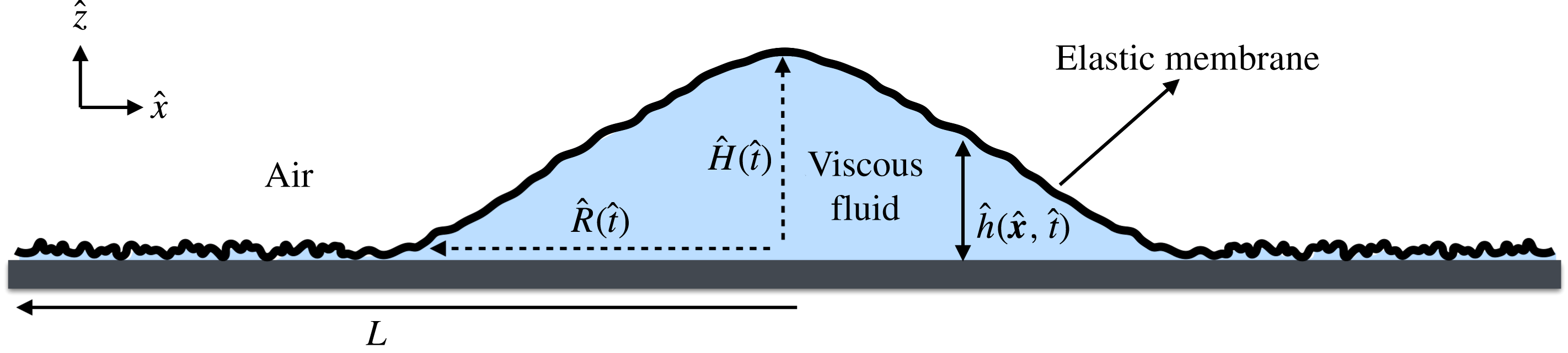
Reference Pihler-Puzović, Juel, Peng, Lister and Heil2015). Thus, we suspect that any presence of fluctuations will cause local changes in the curvature, which will alter the sheet dynamics. To challenge this hypothesis, we consider the elastohydrodynamic analogue to Tanner’s law i.e. a fluid filled blister with an elastic interface that deforms onto a pre-wetted substrate in the presence of fluctuations (see figure 1). The blister is characterized by its maximum height
 ${\hat{H}}(\hat{t})$
at its centre of mass and the spreading radius defined as
 $\hat{R}(\hat{t})$
.
A schematic of the fluid filled blister that has an elastic interface with a bending rigidity, placed on a pre-wetted solid substrate with a microscopic film of height
 $\hat{\unicode[STIX]{x1D716}}$
. The blister is described by its height field
 ${\hat{h}}(\hat{\boldsymbol{x}},\hat{t})$
and has a characteristic height
 ${\hat{H}}(\hat{t})$
and spreading radius
 $\hat{R}(\hat{t})$
. Note that the
 $\hat{x}$
-axis is here compressed by a factor
 $h_{0}/L\ll 1$
.

2.1 Mathematical model
The viscous fluid flow in the gap between the wall and the sheet is described by lubrication theory (Batchelor Reference Batchelor1967; Oron, Davis & Bankoff Reference Oron, Davis and Bankoff2015) as we consider a blister with a lateral extent (
 $L$
) that is much greater than its height
 ${\hat{h}}={\hat{h}}(\hat{x},{\hat{y}},\hat{t})={\hat{h}}(\hat{\boldsymbol{x}},\hat{t})$
with
 $\hat{\unicode[STIX]{x1D735}}{\hat{h}}\ll 1$
i.e. we only consider long wavelength fluctuations. The elastic interface has a bending stiffness
 $B=Eb^{3}/(12(1-\unicode[STIX]{x1D708}))$
with
 $E$
the Young’s modulus,
 $b$
the thickness of the elastic sheet and
 $\unicode[STIX]{x1D708}$
the Poisson ratio. The pressure
 $\hat{p}=\hat{p}(\hat{\boldsymbol{x}},\hat{t})=B\hat{\unicode[STIX]{x1D6FB}}^{4}{\hat{h}}(\hat{\boldsymbol{x}},\hat{t})$
is given by transverse force balance on the sheet (Landau & Lifshitz Reference Landau and Lifshitz1986) and we consider a sheet with small deflections compared to its thickness, allowing us to neglect in-plane stresses and tension in the solid material. The bending pressure together with the inclusion of a stochastic stress term in the Navier–Stokes equations result in a Fokker–Planck-like equation for the spatio-temporal viscous film (Davidovitch et al.
Reference Davidovitch, Moro and Stone2005; Grün et al.
Reference Grün, Mecke and Rauscher2006),
 $$\begin{eqnarray}\frac{\unicode[STIX]{x2202}{\hat{h}}(\hat{\boldsymbol{x}},\hat{t})}{\unicode[STIX]{x2202}\hat{t}}=\hat{\unicode[STIX]{x1D735}}\boldsymbol{\cdot }\left(\frac{{\hat{h}}^{3}(\hat{\boldsymbol{x}},\hat{t})}{12\unicode[STIX]{x1D707}}\hat{\unicode[STIX]{x1D735}}\hat{p}(\hat{\boldsymbol{x}},\hat{t})+\unicode[STIX]{x1D6E4}{\hat{h}}(\hat{\boldsymbol{x}},\hat{t})^{3/2}\hat{\unicode[STIX]{x1D702}}(\hat{\boldsymbol{x}},\hat{t})\right)\end{eqnarray}$$
assuming no-slip at the two solid surfaces. The last term on the right-hand side is unconventional and incorporates a random current that acts as a driving force. This multiplicative conserved noise term for thin film flow only depends on
 $\hat{\boldsymbol{x}}$
and
 $\hat{t}$
, which can formally be derived by Itô and Stratonovich calculus by including an additional symmetric random stress term into the Navier–Stokes equations, for details see Grün et al. (Reference Grün, Mecke and Rauscher2006). The pre-factor multiplying the noise term is
 $\unicode[STIX]{x1D6E4}=\sqrt{2k_{b}T/12\unicode[STIX]{x1D707}},$
with the Boltzmann constant
 $k_{b}$
, the temperature
 $T$
and the spatio-temporal Gaussian white noise
 $\hat{\unicode[STIX]{x1D702}}=\hat{\unicode[STIX]{x1D702}}(\hat{\boldsymbol{x}},\hat{t})$
with zero mean and unit variance. The gradient operator
 $\hat{\unicode[STIX]{x1D735}}$
is in one dimension
 $\unicode[STIX]{x2202}/\unicode[STIX]{x2202}\hat{x}$
and in two dimensions
 $[\unicode[STIX]{x2202}/\unicode[STIX]{x2202}\hat{x},\unicode[STIX]{x2202}/\unicode[STIX]{x2202}{\hat{y}}]$
. We neglect any influence of gravity, as we only consider flows at a length scale that is much smaller than the ’elasto-gravity’ length
 $(B/\unicode[STIX]{x1D70C}g)^{1/4}$
, where
 $\unicode[STIX]{x1D70C}$
is the density and
 $g$
is the gravitational acceleration (Lister et al.
Reference Lister, Peng and Neufeld2013). Linear analysis of (2.1) shows that it indeed recovers the analytical expression for the structure function (Grün et al.
Reference Grün, Mecke and Rauscher2006), as confirmed in simulations. We expect that the influence of fluctuations on the blister dynamics will increase in time as its curvature decreases, contrary to the coarsening of a capillary film where fluctuations are essential at short times (Nesic et al.
Reference Nesic, Cuerno, Moro and Kondic2015b
; Diez et al.
Reference Diez, Gonzalez and Fernandez2016). Thus, to accurately describe the blister dynamics we must capture the spatio-temporal interplay between its nonlinear contribution in height and the multiplicative noise from fluctuations in (2.1), for which an analytical solution is unfeasible. We make (2.1) non-dimensional by scaling;
 $\boldsymbol{x}=\hat{\boldsymbol{x}}/L$
with the maximum blister extent
 $L$
, the height
 $h={\hat{h}}/h_{0}$
with the maximum height of the blister at
 $\hat{t}=0$
i.e.
 $h_{0}=\max ({\hat{h}}(0,\hat{\boldsymbol{x}}))$
and scale time with
 $t=\hat{t}/\unicode[STIX]{x1D70F}=t/12\unicode[STIX]{x1D707}L^{6}/h_{0}^{3}B$
giving the non-dimensional stochastic elastohydrodynamic thin film equation,
 $$\begin{eqnarray}\frac{\unicode[STIX]{x2202}h(\boldsymbol{x},t)}{\unicode[STIX]{x2202}t}=\unicode[STIX]{x1D735}\boldsymbol{\cdot }(h^{3}(\boldsymbol{x},t)\unicode[STIX]{x1D6FB}^{5}h(\boldsymbol{x},t))+N\times \unicode[STIX]{x1D735}\boldsymbol{\cdot }(h(\boldsymbol{x},t)^{3/2}\unicode[STIX]{x1D702}(\boldsymbol{x},t)).\end{eqnarray}$$
One non-dimensional number appears in the equation,
 $N=\sqrt{(2k_{B}TL^{2})/Bh_{0}^{2}}$
that gives the ratio between the force generated by the thermal fluctuations and the elastic bending force from membrane deformation.
2.2 Numerical simulations
To describe the deformation and spreading of the blister we deploy scaling analysis and perform numerical simulations of (2.2) in one and two dimensions by using the finite element method (Amberg, Tönhardt & Winkler Reference Amberg, Tönhardt and Winkler1999), giving the height field as
 $h(x,t)$
and
 $h(x,y,t)$
, respectively. The deterministic parts of (2.2) are solved implicitly (Boyanova, Do-Quang & Neytcheva Reference Boyanova, Do-Quang and Neytcheva2012; Carlson & Mahadevan Reference Carlson and Mahadevan2015a
), while the noise term
 $\unicode[STIX]{x1D702}(\boldsymbol{x},t)$
is treated explicitly as in Nesic et al. (Reference Nesic, Cuerno, Moro and Kondic2015b
). The numerical simulations are complemented by an initial condition for the blister height
 $h(0,\boldsymbol{x})=\unicode[STIX]{x1D716}+(1-\tanh (50(x^{2}+y^{2})))$
, where
 $\unicode[STIX]{x1D716}$
is the pre-wetted layer and pinned boundary conditions are imposed at the edge
 $\unicode[STIX]{x1D6E4}$
i.e.
 $h|_{\unicode[STIX]{x1D6E4}}(\boldsymbol{x},t)=h|_{\unicode[STIX]{x1D6E4}}(\boldsymbol{x},t=0),\unicode[STIX]{x1D6FB}^{2}h|_{\unicode[STIX]{x1D6E4}}\boldsymbol{\cdot }\boldsymbol{n}=p|_{\unicode[STIX]{x1D6E4}}=0$
, with the boundary normal
 $\boldsymbol{n}$
. The results presented here are averages of 20 two-dimensional simulations and 40 simulations in one dimension, where a single run has a computational time of approximately four weeks on a single CPU.
3 Results
3.1 Two-dimensional simulations
We investigate the influence of fluctuations on the elastic interface dynamics by solving (2.2) with
 $N=0$
and
 $N=1$
for a two-dimensional geometry, providing a three-dimensional description of the film. A direct comparison of the deterministic (
 $N=0$
) and stochastic (
 $N=1$
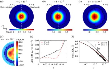
) simulation is shown in figure 2(a–c), where we first notice that the two blisters appear to evolve in a similar fashion. However, subtracting the two height profiles (figure 2
d) shows that the fluctuations affect the shape of the blister’s leading edge, where a precursor-like film is formed ahead of its bulk as the elastic interface peels away from the pre-wetted substrate, see figure 2(e). The blister dynamics appears to adopt a self-similar profile and the extraction of its height
 $H(t)$
in figure 2(f) shows that the deterministic simulation
 $N=0$
follows a power-law behaviour
 $H(t)\sim t^{-2/11}$
that is disturbed as
 $N>0$
, see figure 2(f).
Two-dimensional simulations of (2.2), which represents the three-dimensional dynamics height field
 $h(\boldsymbol{x},t)=h(x,y,t)$
of the elastic blister. The simulations for
 $N=\sqrt{(2k_{B}TL^{2})/\unicode[STIX]{x1D707}h_{0}^{2}}$
is the average over 20 simulations. (a–c) The spatio-temporal blister dynamics. (a,d) Deterministic simulation with
 $N=0$
. (c,f) Inclusion of noise with
 $N=1$
. The solid contour line shows the height
 $h(x,t)=3\times \unicode[STIX]{x1D716}=0.03$
, which is three times the height of the pre-wetted film layer
 $\unicode[STIX]{x1D716}$
. (d) To illustrate the difference between the deterministic and stochastic dynamics, we subtract the height profile for
 $N=1$
from
 $N=0$
i.e.
 $\unicode[STIX]{x0394}h(\boldsymbol{x},t)=h_{N=0}-\langle h\rangle _{N=1}$
at
 $t=1.4\times 10^{-4}$
, showing that a precursor-like film is formed ahead of the bulk of the blister. (e) We magnify the spreading front in the area denoted by the dashed lines in (d), to show the local change in curvature and peeling of the elastic interface from the pre-wetted substrate. (f) The spatio-temporal dynamics in (a–c) suggests that the blister adopts to a self-similar profile. We extract
 $H(t)=\max (h(\boldsymbol{x},\boldsymbol{t}))$
, located at the
 $\boldsymbol{x}$
-position of the blister’s centre of mass. By plotting
 $H(t)$
on a logarithmic axis we show that for
 $N=0$
the height evolves as
 $H(t)\sim t^{-2/11}$
as in (3.1), which is disturbed by the inclusion of noise
 $N=1$
.

To understand the blister dynamics in figure 2 we use a scaling analysis (Davidovitch et al.
Reference Davidovitch, Moro and Stone2005; Lister et al.
Reference Lister, Peng and Neufeld2013), where we start by looking at the limit where fluctuations can be ignored as
 $N=0$
i.e. purely deterministic dynamics. In this limit, the spreading of the blister is slow and has a nearly uniform pressure
 $\hat{p}=\hat{p}_{0}=B\hat{\unicode[STIX]{x1D6FB}}^{4}{\hat{h}}(\hat{\boldsymbol{x}},\hat{t})\sim B{\hat{H}}(\hat{t})/\hat{R}^{4}(\hat{t})$
in its bulk (Lister et al.
Reference Lister, Peng and Neufeld2013). By integrating
 $\hat{p}$
we get the blister shape by assuming axial symmetry, as also confirmed in the two-dimensional simulation, and boundary conditions; at the symmetry line
 $\hat{\unicode[STIX]{x1D735}}{\hat{h}}=\hat{\unicode[STIX]{x1D6FB}}^{3}{\hat{h}}=0$
and at the advancing front
 ${\hat{h}}=\hat{\unicode[STIX]{x1D735}}{\hat{h}}=O(\hat{\unicode[STIX]{x1D716}})$
(Lister et al.
Reference Lister, Peng and Neufeld2013). The blister shape combined with the matching of the local travelling-wave solution
 ${\hat{c}}$
gives the speed of the peeling tip
 $\text{d}\hat{R}/\text{d}\hat{t}={\hat{c}}=B\hat{\unicode[STIX]{x1D716}}^{1/2}/12\unicode[STIX]{x1D707}(\hat{\unicode[STIX]{x1D705}}/1.35)^{5/2}$
(Lister et al.
Reference Lister, Peng and Neufeld2013) that is dictated by its local curvature
 $\hat{\unicode[STIX]{x1D705}}$
, the pre-wetted film height
 $\hat{\unicode[STIX]{x1D716}}$
, membrane stiffness
 $B$
and viscosity
 $\unicode[STIX]{x1D707}$
. We scale
 ${\hat{h}}\sim {\hat{H}}(\hat{t}),\hat{\boldsymbol{x}}\sim \hat{R}(\hat{t})$
together with the solution for
 ${\hat{c}}$
and impose mass conservation through a constant film volume
 $\hat{V}=\int _{0}^{L}\int _{0}^{L}({\hat{h}}(\hat{x},\hat{t})-\hat{\unicode[STIX]{x1D716}})\,\text{d}\hat{x}\,\text{d}{\hat{y}}$
(in one dimension given by the constant area
 $\hat{A}=\int _{0}^{L}({\hat{h}}(\hat{x},\hat{t})-\hat{\unicode[STIX]{x1D716}})\,\text{d}\hat{x}$
), which gives the self-similar spreading dynamics for a three-dimensional (axisymmetric) blister
 $$\begin{eqnarray}\hat{R}(\hat{t})=1.57\left(\frac{B^{2}\hat{\unicode[STIX]{x1D716}}}{\unicode[STIX]{x1D707}^{2}}\hat{V}^{5}\hat{t}\right)^{1/22},\quad {\hat{H}}(\hat{t})=\frac{\hat{V}}{\hat{R}^{2}(\hat{t})}.\end{eqnarray}$$
In non-dimensional form this becomes
 $R(t)\approx t^{1/11}$
and
 $H(t)\approx t^{-2/11}$
and in one-dimensional geometries
 $R(t)\approx t^{2/17}$
and
 $H(t)\approx t^{-2/17}$
. This is the elastohydrodynamic analogue to Tanner’s law for capillary spreading (two dimensions:
 $R(t)\sim t^{1/10}$
, one dimension:
 $R(t)\sim t^{1/7}$
), but contrasts the classical solution with different exponents in time. Our self-similar solution is verified in the numerical simulation shown in figure 2(f) with
 $N=0$
. However, for
 $N>0$
the spreading dynamics is influenced by the fluctuations.
Next, we examine the flow regime where the fluctuation effects dominate over the bending rigidity in (2.1) i.e. a flaccid membrane, and look for its self-similar solution. The stochastic term scales as
 $\hat{\unicode[STIX]{x1D702}}(\hat{\boldsymbol{x}},\hat{t})\sim 1/(\sqrt{\text{d}\hat{t}}\,\text{d}\hat{x})$
(in one-dimensional geometries as
 $\hat{\unicode[STIX]{x1D702}}(\hat{x},\hat{t})\sim 1/\sqrt{\text{d}\hat{t}\,\text{d}\hat{x}{\hat{w}}}$
, with
 ${\hat{w}}$
as the in-plane depth) (Davidovitch et al.
Reference Davidovitch, Moro and Stone2005) in (2.1), which combined with the mass conservation equation for the film gives,
 $$\begin{eqnarray}\hat{R}_{s}(\hat{t})=\left(\frac{2k_{b}T\hat{V}}{12\unicode[STIX]{x1D707}}\hat{t}\right)^{1/6},\quad {\hat{H}}_{s}(\hat{t})=\frac{\hat{V}}{\hat{R}_{s}^{2}(\hat{t})}.\end{eqnarray}$$
In non-dimensional form this becomes
 $R_{s}(t)\approx (N^{2}t)^{1/6}$
and
 $H_{s}\approx R_{s}^{-2}(t)\approx (N^{2}t)^{-1/3}$
and in one-dimensional geometries
 $R_{s}(t)\approx (N^{2}t/w)^{1/4}$
and
 $H_{s}(t)\approx (N^{2}t/w)^{-1/4}$
where
 $w={\hat{w}}/L$
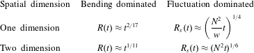
, similar to the capillary films in Davidovitch et al. (Reference Davidovitch, Moro and Stone2005). These scaling predictions (3.1) and (3.2) have been summarized in table 1, for one- and two-dimensional geometries.
Non-dimensional scaling laws for the spreading radius
 $R(t)$
and height
 $H(t)$
of the blister, using the scaling:
 $h={\hat{h}}/h_{0}$
,
 $x=\hat{x}/L$
,
 $t=\hat{t}/\unicode[STIX]{x1D70F}=t/(12\unicode[STIX]{x1D707}L^{6})/h_{0}^{3}B$
, where
 $B$
is the bending stiffness,
 $\unicode[STIX]{x1D707}$
the viscosity,
 $L$
the lateral extent of the blister and
 $h_{0}$
its maximum height at
 $\hat{t}=0$
. The non-dimensional number
 $N=\sqrt{(2k_{b}TL^{2})/Bh_{0}^{2}}$
gives the ratio of the force from thermal fluctuations and the elastic bending force, where
 $k_{b}$
is the Boltzmann constant and
 $T$
the temperature. In one-dimensional geometries we also have the scaled in-plane width
 $w={\hat{w}}/L$
, which appear in the pre-factor for the scaling law.

3.2 One-dimensional simulations
In order to characterize the influence of
 $N=\sqrt{(2k_{b}TL^{2})/Bh_{0}^{2}}$
on the blister dynamics, we systematically vary
 $N$
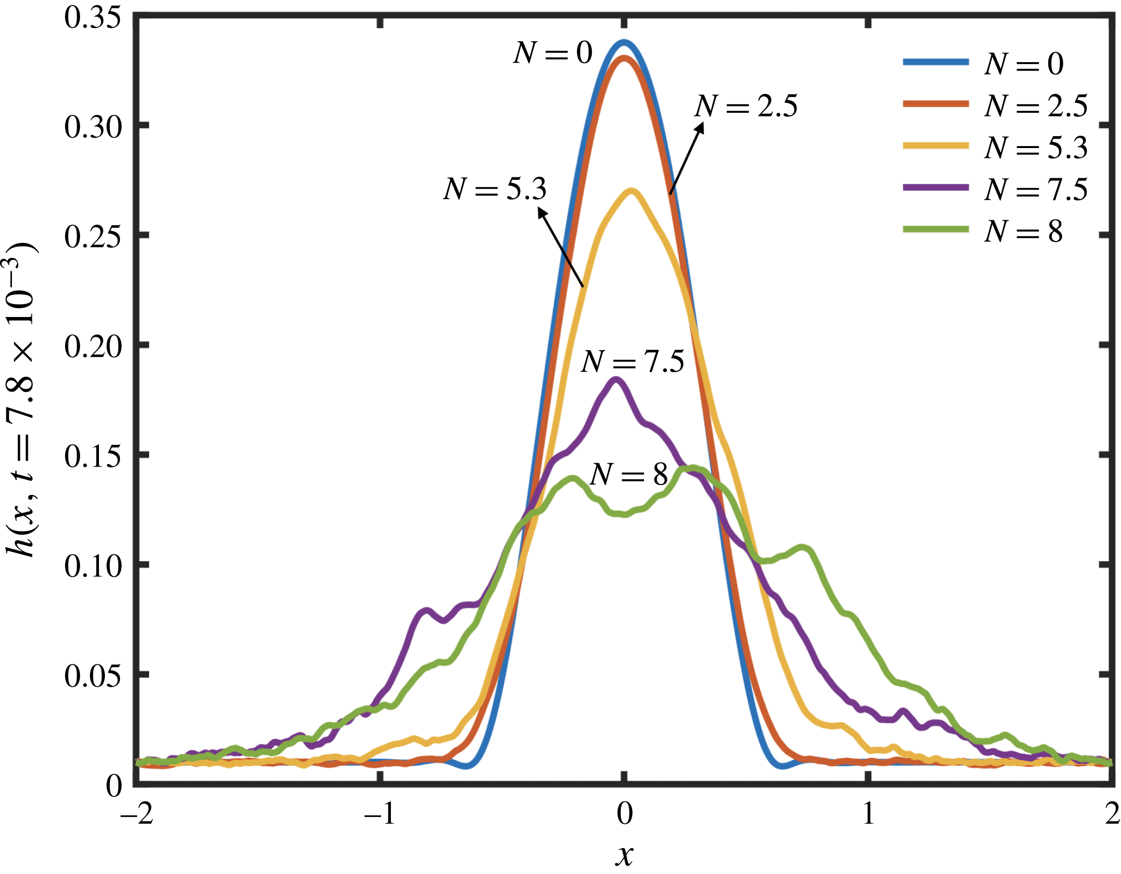
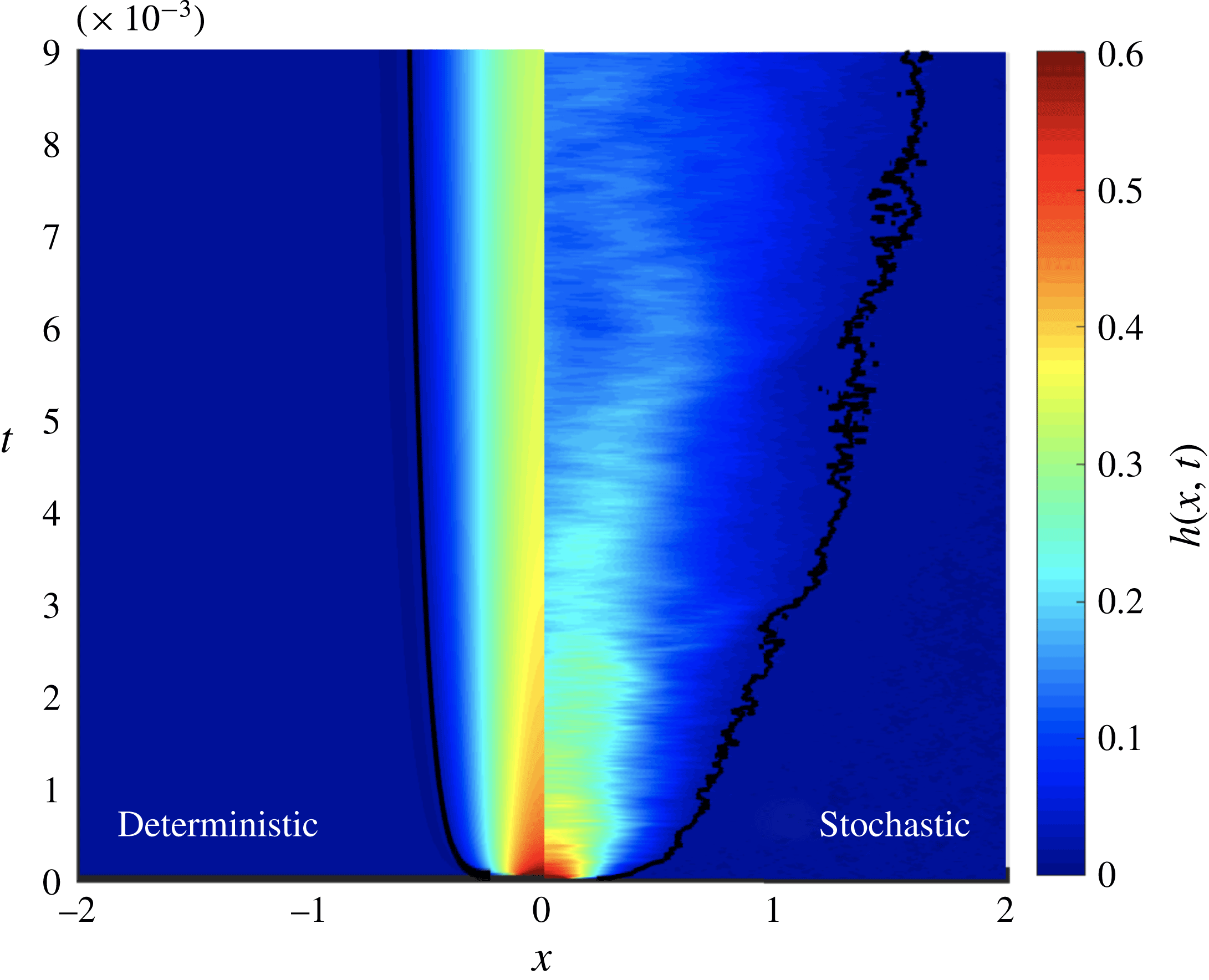
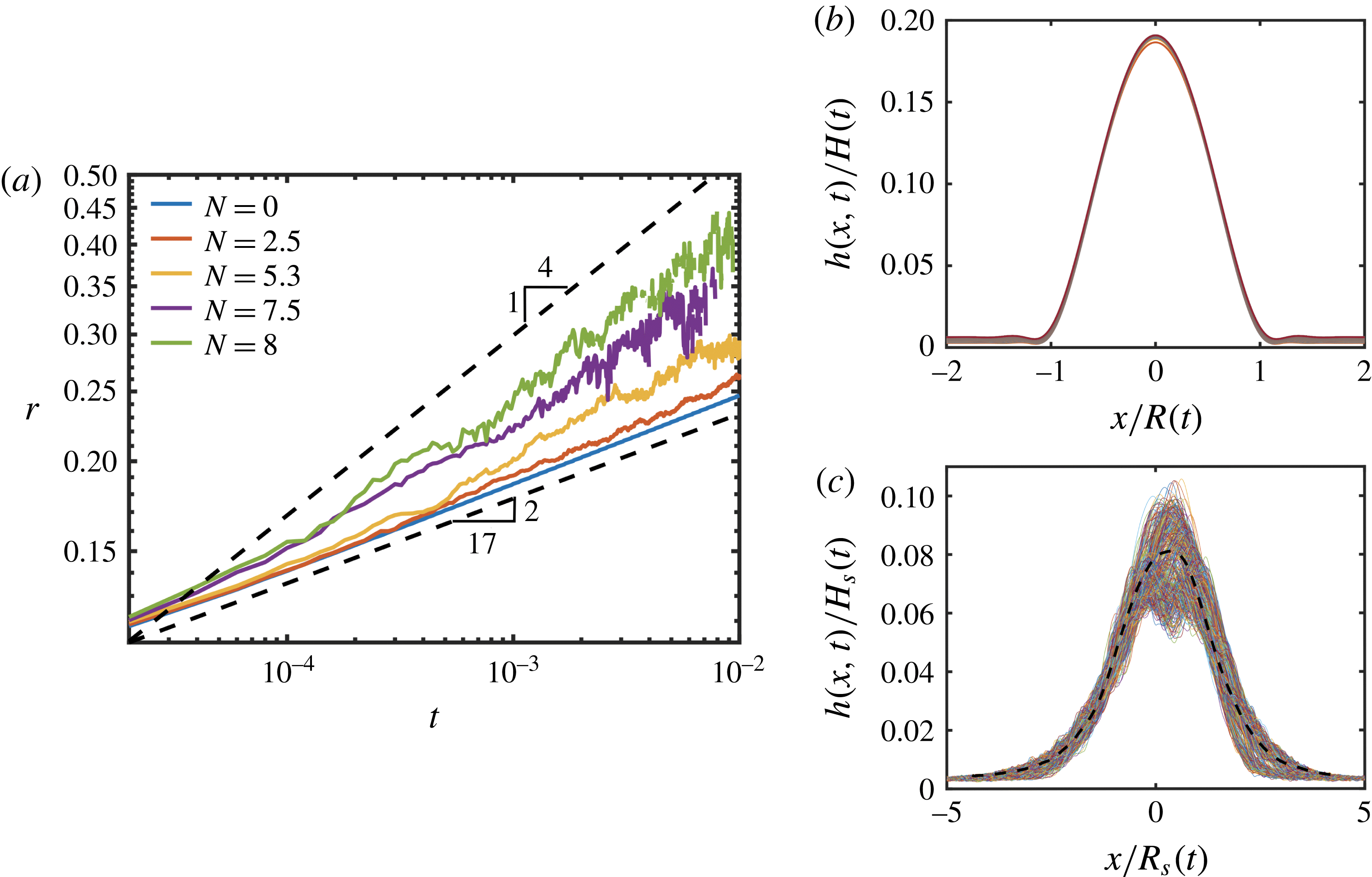
in a one-dimensional geometry, see figures 3 and 4. It is clear that fluctuations can significantly speed up the spreading dynamics and we observe a dramatic change in blister shapes. By tracking the spatio-temporal blister shape in figure 4 we identify two distinct regimes, one for the elastohydrodynamic Tanner’s law (3.1) and a stochastic spreading regime (3.2), see table 1.
We extract the spreading radius from the simulations in figure 3 by the averaged second moment to describe the advancing front
 $r=\langle [(1/A)\int h(x,t)(x-X)^{2}\,\text{d}x]^{1/2}\rangle$
with
 $X=[\int xh(x,t)\,\text{d}x]/A$
(Davidovitch et al.
Reference Davidovitch, Moro and Stone2005; Nesic et al.
Reference Nesic, Cuerno, Moro and Kondic2015b
). The numerical simulations show that for
 $N=0$
the spreading recovers the deterministic self-similar profile in (3.1) and as
 $N\geqslant 5.3$
the advancing front adopts the stochastic dynamics predicted by (3.2). These regimes are further illustrated by the collapse of blister shapes onto a universal curve by rescaling its numerical profiles with
 $x/R(t),h/H(t)$
for
 $N=0$
see figure 5(b) and
 $x/R_{s}(t),h/H_{s}(t)$
for
 $N=8$
see figure 5(c).
The average of 40 numerical simulations of (2.2) in one dimension with
 $N\in [0,2.5,5.3,7.5,8]$
at time
 $t=7.8\times 10^{-3}$
, using the scaling for
 $h(x,t)={\hat{h}}(\hat{x},\hat{t})/h_{0}$
and
 $x=\hat{x}/L$
. Note that the
 $x$
-axis is here compressed by a factor
 $h_{0}/L\ll 1$
. We would like to note that the non-dimensional gradient
 $\unicode[STIX]{x2202}h/\unicode[STIX]{x2202}x$
for
 $N=8$
has a maximal absolute value
 $\max (|\unicode[STIX]{x2202}h/\unicode[STIX]{x2202}x|)\approx O(1)$
for each simulation throughout time and our long wave approximation is still valid as we have
 $\unicode[STIX]{x2202}{\hat{h}}/\unicode[STIX]{x2202}\hat{x}=(h_{0}/L)\unicode[STIX]{x2202}h/\unicode[STIX]{x2202}x\ll 1$
.

Comparison of the spatio-temporal blister dynamics for
 $N=0$
(left side) and
 $N=8$
(right side). The solid line indicates the height
 $h(x,t)=3\times \unicode[STIX]{x1D716}=0.03$
, which is three times the pre-wetted film height
 $\unicode[STIX]{x1D716}$
and the results are obtained from an average of 40 simulations of (2.2) in one dimension.

(a) The extracted spreading radius
 $r$
in logarithmic axis for
 $N\in [0,2.5,5.3,7.5,8]$
, the dashed lines illustrate the spreading laws in (3.1) and (3.2). (b) The height profiles for the times
 $t=[1:2\times 10^{-2}:10]\times 10^{-3}$
with
 $N=0$
are rescaled as
 $x/R(t)$
and
 $h/H(t)$
in (3.1). (c) The average height profile for the times
 $t=[1:2\times 10^{-2}:10]\times 10^{-3}$
with
 $N=8$
are rescaled as
 $x/R_{s}(t)$
and
 $h/H_{s}(t)$
in (3.2), where the dashed line is the mean of the scaled profile. The results are obtained from an average of 40 simulations of (2.2) in one dimension.

3.3 Regime transition
Our theoretical model is supported by simulations of (2.2) in both one and two dimensions, but limited to fluctuations with a wavelength
 $\unicode[STIX]{x1D706}\ll h/\unicode[STIX]{x1D735}h$
, which is asymptotically correct as
 $\unicode[STIX]{x1D735}h\rightarrow 0$
for
 $t\rightarrow \infty$
. To determine the threshold in the spreading radius for when the stochastic effects will dominate the flow, we use the scaling prediction in (3.2) and compare the magnitude of the two terms on the right-hand side of (2.2). We start by estimating the contribution from interface bending, which scales as
 $\unicode[STIX]{x1D735}\boldsymbol{\cdot }(h^{3}\unicode[STIX]{x1D6FB}^{5}h)\sim R^{-14}$
(in one dimension
 ${\sim}R^{-10}$
) and the stochastic term scales as
 $\unicode[STIX]{x1D735}\boldsymbol{\cdot }(Nh^{3/2}\unicode[STIX]{x1D702})\sim N^{2}R^{-8}$
(in one dimension
 ${\sim}N^{2}w^{-1}R^{-5}$
). Next, we balance these two terms, giving the condition on the spreading radius
 $R>1/N^{1/3}$
(in one dimension
 $R>(w/N^{2})^{1/5}$
) for stochastic effects to dominate the flow. The numerical simulations in figure 5 illustrates this transition in regimes for
 $N=[5.3,7.5,8]$
, where there is a clear change in slope for
 $R\approx 0.2$
in accordance with our analysis. In the simulations, we vary
 $N\in [0{-}8]$
, which corresponds to a membrane with a bending stiffness
 $B\in [10{-}100]k_{b}T$
, at 300 k with
 $k_{b}T=4\times 10^{-21}~\text{Nm}$
, a size
 $L=5~\unicode[STIX]{x03BC}\text{m}$
and height
 $h_{0}=10~\text{nm}$
, which gives
 $N\in 2{-}15$
in accordance with the simulations presented in figures 2–5. In one-dimensional geometries we notice that the in-plane depth
 $w$
influences the transition from deterministic to stochastic spreading dynamics.
3.4 Scaling estimates of other physical effects
Membrane dynamics at microscopic length scales can also be influenced by additional forces arising from the molecular interaction between the material composing the interface and the solid substrate e.g. a van der Waals disjoining pressure
 $\hat{p}_{vdW}=A/3{\hat{h}}^{3}$
, where
 $A$
is the Hamaker constant. In addition, biological adhesion phenomena often involve the attachment of long proteins that can influence the front propagation and by assuming these to be like Hookean springs they give a contribution to the pressure
 $\hat{p}_{s}=K(1-{\hat{h}}/l_{i})$
(Leong & Chiam Reference Leong and Chiam2010; Carlson & Mahadevan Reference Carlson and Mahadevan2015b
), with the effective spring stiffness
 $K$
and
 $l_{i}$
is the natural protein length. To observe the stochastic regime in these other flow situations, their contribution to the pressure must be much smaller than the stochastic contribution in (2.2).
The disjoining pressure would add a contribution to the right-hand side of (2.2) that scales as
 $\unicode[STIX]{x1D735}\boldsymbol{\cdot }(h^{3}\unicode[STIX]{x1D735}p_{vdW})=\unicode[STIX]{x1D6E4}\unicode[STIX]{x1D735}\boldsymbol{\cdot }(h^{-1}\unicode[STIX]{x1D735}h)\sim \unicode[STIX]{x1D6E4}R^{-2}$
where
 $\unicode[STIX]{x1D6E4}=AL^{4}/Bh_{0}^{4}$
is a non-dimensional number for the ratio between van der Waals adhesion energy and the bending energy. Performing the same scaling analysis for the contribution from the spring pressure gives
 $\unicode[STIX]{x1D735}\boldsymbol{\cdot }(h^{3}\unicode[STIX]{x1D735}p_{s})=S\unicode[STIX]{x1D735}\boldsymbol{\cdot }(h^{3}\unicode[STIX]{x1D735}h)\sim SR^{-10}$
(in one dimension
 ${\sim}SR^{-6}$
) with
 $S=KL^{4}/B$
a non-dimensional number for the ratio of the spring pressure and the bending pressure. We individually compare the magnitude of the stochastic fluctuations with the deterministic contributions from these additional physical effect. The contribution from the van der Waals pressure gives
 $R<(N^{2}/\unicode[STIX]{x1D6E4})^{1/6}$
(in one dimension
 $R<(N^{2}/\unicode[STIX]{x1D6E4}w)^{1/3}$
) and the spring pressure gives
 $R>(S/N^{2})^{1/2}$
(in one dimension
 $R>(Sw/N^{2})$
). A typical value for the Hamaker constant is
 $A\approx 10k_{b}T$
with
 $\unicode[STIX]{x1D6E4}\in [6.2-0.62]\times 10^{6}$
. If we assume a spring adhesion phenomenon (Carlson & Mahadevan Reference Carlson and Mahadevan2015a
) mediated by proteins with a number density
 $C\approx 100~(\unicode[STIX]{x03BC}\text{m})^{-2}$
and a stiffness
 $\unicode[STIX]{x1D6FE}\approx 10^{-7}~\text{N}~\text{m}^{-1}$
, we get that
 $K=C\unicode[STIX]{x1D6FE}=10^{7}~\text{N}~\text{m}^{-3}$
and
 $S\in [2{-}15]$
.
4 Conclusions
Adhesion of biological membranes is primarily modelled as springs (Reister-Gottfried et al.
Reference Reister-Gottfried, Sengupta, Lorz, Sackmann, Seifert and Smith2008; Leong & Chiam Reference Leong and Chiam2010) where our stochastic elastohydrodynamic model gives an accurate description of the viscous flow in the membrane gap that may help rationalize new regimes complementing those predicted by over-damped dynamics (Reister-Gottfried et al.
Reference Reister-Gottfried, Sengupta, Lorz, Sackmann, Seifert and Smith2008). A word of caution, as the model presented here is only valid for small deflections of the elastic membrane compared to its thickness. There are internal structures in a cell including a cortex shell of several hundred nanometres (Carvalho et al.
Reference Carvalho, Tsai, Lees, Voituriez, Koenderink and Sykes2013; Cartagena et al.
Reference Cartagena-Rivera, Logue, Waterman and Chadwick2016) in addition to the plasma membrane, which generate an effective elastic interface that would be much thicker than the fluid film of a few tens of nanometres separating the cell from the substrate. If we were to describe tension effects in the membrane, we would need to describe the in-plane stresses and solve the Föppl–von Kármán equation for the membrane (Lister et al.
Reference Lister, Peng and Neufeld2013; Peng et al.
Reference Peng, Pihler-Puzović, Juel, Heil and Lister2015; Pihler-Puzović et al.
Reference Pihler-Puzović, Juel, Peng, Lister and Heil2015). At a scaling level, we can distinguish the bending regime, described above, from a tension regime by using scaling analysis following Lister et al. (Reference Lister, Peng and Neufeld2013) for a blister with a constant volume, which gives
 $R\sim t^{1/16}$
, contrasting (3.1). However, obtaining a numerical solution to the Föppl–von Kármán equation coupled with fluid flow and a noise term is considered to be a daunting challenge. The fluctuations are modelled here as white Gaussian noise, while other systems might have different noise characteristics leading to a finite correlation length i.e. coloured noise, which can be determined from experiments (Diez et al.
Reference Diez, Gonzalez and Fernandez2016). It would also be very interesting to explore how these fluctuations could affect the instability threshold of forced elastic fronts in Hele-Shaw geometries (Juel et al.
Reference Juel, Pihler-Puzović and Heil2018).
The presented mathematical model provides a minimal and general theoretical skeleton for a description of stochastic elastohydrodynamic flows. By combining a scaling analysis and numerical simulations, we find two spreading regimes; an elastohydrodynamic analogue to Tanner’s law for capillary spreading and a stochastic dynamics, with a distinct criterion predicting the transition between these two regimes as also observed in the numerical simulations. Fluctuations alter the local curvature of the advancing front, leading to the peeling of the elastic interface and the formation of a precursor-like film advancing ahead of the bulk blister. This model is likely useful beyond the spreading of an elastic blisters as it sets the stage for the quantification of flow, elasticity, adhesion and stochastic effects in broader aspects of bio-inspired adhesion phenomena.
Acknowledgements
I would like to thank Dr M. Do-Quang for invaluable assistance in linking femLego with Boost. The financial support from the Norwegian Research Council – Project number 263056 and the Chair Total at ESPCI Paris are gratefully acknowledged.