2.1. Governing equations

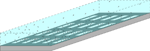
We consider a laminar pressure-driven fluid flow, contaminated with soluble surfactant, in a channel bounded between two SHS that are periodic in the streamwise and spanwise directions, as illustrated in figure 1. We use hats to indicate dimensional quantities. The streamwise, wall-normal and spanwise directions are denoted by $\hat {x}$, $\hat {y}$ and $\hat {z}$ coordinates, where $\hat {\boldsymbol {x}} = (\hat {x},\hat {y},\hat {z})$ is the space vector and $\hat {t}$ is time. Assuming that the fluid is incompressible and Newtonian, we introduce the velocity vector $\hat {\boldsymbol {u}}=(\hat {u}(\hat {\boldsymbol {x}}, \hat {t}),\hat {v}(\hat {\boldsymbol {x}}, \hat {t}),\hat {w}(\hat {\boldsymbol {x}}, \hat {t}))$, pressure field $\hat {p}(\hat {\boldsymbol {x}}, \hat {t})$, bulk surfactant concentration field $\hat {c}(\hat {\boldsymbol {x}}, \hat {t})$ and interfacial surfactant concentration field $\hat {\varGamma }(\hat {x},\hat {z}, \hat {t})$. The streamwise length of the channel is $2 \hat {L}_x$ and the periodic cell has streamwise (spanwise) period length $2 \hat {P}_x$ ($2 \hat {P}_z$), liquid–gas interface length (width) $2 \phi _x \hat {P}_x$ ($2 \phi _z \hat {P}_z$) and gas fraction $\phi _x$ ($\phi _z$). The channel height is $2\hat {H}$. The liquid–gas interfaces (plastrons) can protrude into or out of the gas cavities by an amount that varies along the channel with the liquid and gas pressures (see Lee et al. Reference Lee, Choi and Kim2016); however, for the sake of simplicity, we assume here that all the plastrons are flat. The SHS are made up of $2N+1$ periodic cells in the streamwise direction. For $n \in \{-N, \ldots, N\}$, the $n$th periodic cell is split into two subdomains along the streamwise direction, similarly to Temprano-Coleto et al. (Reference Temprano-Coleto, Smith, Peaudecerf, Landel, Gibou and Luzzatto- Fegiz2023),

(2.1a)$$\begin{gather} \hat{\mathcal{D}}^n_1 = \{\hat{x}- 2n\hat{P}_x\in [-\phi_x\hat{P}_x, \phi_x\hat{P}_x]\} \times \{\hat{y}\in [0, 2 \hat{H}]\} \times \{\hat{z} \in [- \hat{P}_z, \hat{P}_z]\}, \end{gather}$$

(2.1b)$$\begin{gather}\hat{\mathcal{D}}^n_2 = \{\hat{x}- 2n\hat{P}_x\in [\phi_x \hat{P}_x, (2 - \phi_x)\hat{P}_x]\} \times \{\hat{y}\in [0, 2 \hat{H}]\} \times \{\hat{z} \in [- \hat{P}_z, \hat{P}_z]\}. \end{gather}$$

At the SHS, $\hat {y} = 0$ and $\hat {y}= 2\hat {H}$, we define the $n$th interface, ridge and solid region as

(2.2a)$$\begin{gather} \hat{\mathcal{I}}^n = \{\hat{x} - 2n\hat{P}_x \in [-\phi_x\hat{P}_x, \phi_x\hat{P}_x]\} \times \{\hat{z} \in [- \phi_z \hat{P}_z, \phi_z \hat{P}_z]\}, \end{gather}$$

(2.2b)$$\begin{gather}\hat{\mathcal{R}}^n = \{\hat{x}- 2n\hat{P}_x \in [-\phi_x\hat{P}_x,\phi_x\hat{P}_x]\} \times \{\hat{z} \in [- \hat{P}_z,-\phi_z \hat{P}_z]\cup [\phi_z \hat{P}_z,\hat{P}_z]\}, \end{gather}$$

(2.2c)$$\begin{gather}\hat{\mathcal{S}}^n = \{\hat{x}- 2n\hat{P}_x \in [\phi_x\hat{P}_x, (2 - \phi_x)\hat{P}_x]\} \times \{\hat{z} \in [- \hat{P}_z, \hat{P}_z]\}. \end{gather}$$

Figure 1.

A schematic illustrating the multiple length scales present in a channel flow bounded by streamwise- and spanwise-periodic SHS. (a) The surfactant flux varies in the streamwise direction, $\hat {\chi }$, and time, $\hat {\tau }$, over the length of the channel, $2\hat {L}_x$. (b) Over each period, the concentration of surfactant varies quasi-steadily in the streamwise direction, $\hat {x}$. Multiple periodic cells are shown, each with a varying concentration of surfactant. The origin of the Cartesian coordinate system, $\hat {\boldsymbol {x}}=\boldsymbol {0}$, is placed in the middle of the interface of the central period, at a distance $\hat {L}_x$ along the channel. (c) A periodic cell, identifying domains 1 and 2 and, at the SHS, the ridge, solid wall and liquid–gas interface. For each periodic cell, the half-channel height is $\hat {H}$, the streamwise (spanwise) gas fraction is $\phi _z$ ($\phi _z$) and the streamwise (spanwise) period length is $2\hat {P}_x$ ($2\hat {P}_z$).

The steady equations that govern the fluid and surfactant in each periodic cell are described in detail by Tomlinson et al. (Reference Tomlinson, Gibou, Luzzatto-Fegiz, Temprano-Coleto, Jensen and Landel2023a). This paper investigates the situation where the concentration field exhibits period-to-period variations, as illustrated in figure 1. This variability arises, for instance, if a surfactant source is introduced at the channel inlet. As the flow carries the excess surfactant downstream, the excess surfactant interacts with the SHS, changing the local drag, velocity field and other pertinent quantities for applications in time and space. Below, we highlight differences from Tomlinson et al. (Reference Tomlinson, Gibou, Luzzatto-Fegiz, Temprano-Coleto, Jensen and Landel2023a) due to the unsteady transport of surfactant, allowing the total flux of surfactant (that depends on the velocity and concentration fields in each period) to vary over the full length of the channel. The bulk surfactant is coupled to the steady incompressible flow through an unsteady advection–diffusion equation. In $\hat {\mathcal {D}}_1^n$ and $\hat {\mathcal {D}}_2^n$,

(2.3a–c)\begin{equation} \hat{\boldsymbol{\nabla}} \boldsymbol{\cdot} \hat{\boldsymbol{u}} = 0, \quad \hat{\mu} \hat{\nabla}^2 \hat{\boldsymbol{u}}- \hat{\boldsymbol{\nabla}} \hat{p} = \boldsymbol{0}, \quad \hat{D} \hat{\nabla}^2 \hat{c} - \hat{\boldsymbol{u}}\boldsymbol{\cdot}\hat{\boldsymbol{\nabla}} \hat{c} - \hat{c}_{\hat{t}} = 0, \end{equation}

where $\hat {\mu }$ is dynamic viscosity and $\hat {D}$ is the surfactant bulk diffusivity. The interfacial surfactant is coupled to the flow through an unsteady advection–diffusion equation and a linear equation of state and adsorption–desorption kinetics, such that $(\hat {\sigma }_{\hat {x}}, \hat {\sigma }_{\hat {z}}) = (-\hat {A}\hat {\varGamma }_{\hat {x}}, -\hat {A}\hat {\varGamma }_{\hat {z}})$, where $\hat {\sigma }$ is the surface tension and $\hat {A}$ is the surface activity (Manikantan & Squires Reference Manikantan and Squires2020). We linearise the equation of state and adsorption–desorption kinetics, as surfactant concentrations are generally small when surfactant is not artificially added (Manikantan & Squires Reference Manikantan and Squires2020). At $\hat {y} = 0$ ($\hat {y}= 2\hat {H}$) and along $\hat {\mathcal {I}}^n$, the boundary and bulk–interface coupling conditions for surfactant and flow and the interfacial surfactant transport equation are

(2.4a–e)\begin{equation} \left.\begin{gathered} \hat{\mu} \boldsymbol{n}\boldsymbol{\cdot}\hat{\boldsymbol{\nabla}} \hat{u} - \hat{A} \hat{\varGamma}_{\hat{x}} = 0, \quad \hat{v}=0, \quad \hat{\mu} \boldsymbol{n}\boldsymbol{\cdot} \hat{\boldsymbol{\nabla}} \hat{w} - \hat{A} \hat{\varGamma}_{\hat{z}} = 0, \quad \hat{D} \boldsymbol{n}\boldsymbol{\cdot}\hat{\boldsymbol{\nabla}} \hat{c} - \hat{K}_a \hat{c} + \hat{K}_d \hat{\varGamma} =0, \\ \hat{D}_I ( \hat{\varGamma}_{\hat{x}\hat{x}} + \hat{\varGamma}_{\hat{z}\hat{z}} ) + \hat{K}_a \hat{c} - \hat{K}_d \hat{\varGamma} -(\hat{u} \hat{\varGamma})_{\hat{x}} - (\hat{w} \hat{\varGamma})_{\hat{z}} - \hat{\varGamma}_{\hat{t}} = 0, \end{gathered}\right\} \end{equation}

where $\boldsymbol {n}$ is the unit normal to the interface (pointing into the channel), $\hat {D}_I$ is the surfactant interfacial diffusivity, $\hat {K}_a$ is the adsorption rate coefficient and $\hat {K}_d$ is the desorption rate coefficient. At $\hat {y} = 0$ ($\hat {y} = 2\hat {H}$) on $\partial \hat {\mathcal {I}}^n$, there is no flux of surfactant:

(2.5a,b)\begin{equation} \hat{u}\hat{\varGamma} - \hat{D}_I \hat{\varGamma}_{\hat{x}} = 0 \quad \text{at} \ \hat{x} ={\pm} \phi_x \hat{P}_x, \quad \hat{w}\hat{\varGamma} - \hat{D}_I \hat{\varGamma}_{\hat{z}} = 0 \quad \text{at} \ \hat{z} ={\pm} \phi_z \hat{P}_z. \end{equation}

At $\hat {y} = 0$ ($\hat {y} = 2\hat {H}$) along $\hat {\mathcal {R}}^n\cup \hat {\mathcal {S}}^n$, the flow and surfactant boundary conditions are

(2.6a–d)\begin{equation} \hat{u} = 0, \quad \hat{v} =0, \quad \hat{w} = 0, \quad \hat{c}_{\hat{y}} =0. \end{equation}

Next, we define $\hat {\boldsymbol {q}}(\hat {\boldsymbol {x}},\,\hat {t}) = (\hat {u}, \hat {v}, \hat {w}, \hat {p}_{\hat {x}}, \hat {c})$. Throughout $\hat {\mathcal {D}}^n_1$ and $\hat {\mathcal {D}}^n_2$, we assume that the flow and concentration fields are periodic in the spanwise directions,

(2.7)\begin{equation} \hat{\boldsymbol{q}}(\hat{x},\hat{y},-\hat{P}_z,\hat{t}) = \hat{\boldsymbol{q}}(\hat{x},\hat{y},\hat{P}_z,\hat{t}). \end{equation}

Across interfaces between $\hat {\mathcal {D}}_1^n$, $\hat {\mathcal {D}}_2^n$ and $\hat {\mathcal {D}}_1^{n+1}$ the flow and concentration fields are assumed to be continuous between subdomains,

(2.8a)$$\begin{gather} \hat{\boldsymbol{q}}(((2n + \phi_x)\hat{P}_x)^-,\hat{y},\hat{z},\hat{t}) = \hat{\boldsymbol{q}}(((2n + \phi_x)\hat{P}_x)^+,\hat{y},\hat{z} ,\hat{t}), \end{gather}$$

(2.8b)$$\begin{gather}\hat{\boldsymbol{q}}(((2(n+1) -\phi_x)\hat{P}_x)^-,\hat{y},\hat{z},\hat{t}) = \hat{\boldsymbol{q}}(((2(n+1) - \phi_x )\hat{P}_x)^+,\hat{y},\hat{z},\hat{t}). \end{gather}$$

In addition to (2.7)–(2.8), derivatives of $\hat {\boldsymbol {q}}$ should be continuous across subdomains and spanwise periods.

We can integrate (2.3)–(2.7) across the channel to derive equations relating the bulk and interfacial flux of fluid and surfactant, i.e.

(2.9a)$$\begin{gather} \int_{\hat{\mathscr{A}}_n} \hat{c}_{\hat{t}} \, \text{d}\hat{A} + \frac{\text{d}}{\text{d}\hat{x}} \int_{\hat{\mathscr{A}}_n} (\hat{u}\hat{c} - \hat{D} \hat{c}_{\hat{x}}) \, \text{d}\hat{A} - 2 \int_{\hat{\mathscr{I}}_n} (\hat{K}_d \hat{\varGamma} - \hat{K}_a \hat{c}) \, \text{d}\hat{z} = 0 \quad \text{in} \ \hat{\mathcal{D}}_1^n, \end{gather}$$

(2.9b)$$\begin{gather}\int_{\hat{\mathscr{I}}_n} \hat{\varGamma}_{\hat{t}}\, \text{d}\hat{z} + \frac{\text{d}}{\text{d}\hat{x}} \int_{\hat{\mathscr{I}}_n} (\hat{u}\hat{\varGamma} - \hat{D}_I \hat{\varGamma}_{\hat{x}}) \, \text{d}\hat{z} + \int_{\hat{\mathscr{I}}_n} (\hat{K}_d \hat{\varGamma} - \hat{K}_a \hat{c}) \, \text{d}\hat{z} = 0 \quad \text{in} \ \hat{\mathcal{D}}_1^n, \end{gather}$$

(2.9c)$$\begin{gather}\int_{\hat{\mathscr{A}}_n} \hat{c}_{\hat{t}} \, \text{d}\hat{A} + \frac{\text{d}}{\text{d}\hat{x}} \int_{\hat{\mathscr{A}}_n} (\hat{u}\hat{c} - \hat{D} \hat{c}_{\hat{x}}) \, \text{d}\hat{A} = 0 \quad \text{in}\ \hat{\mathcal{D}}_2^n, \end{gather}$$

where $\int _{\hat {\mathscr {A}}_n}{\cdot }\, \textrm {d}\hat {A} \equiv \int _{\hat {z}=-\hat {P}_z}^{\hat {P}_z}\int _{\hat {y}=0}^{2\hat {H}} {\cdot } \, \textrm {d} \hat {y} \, \textrm {d} \hat {z}$ and $\int _{\hat {\mathscr {I}}_n} {\cdot } \, \textrm {d}\hat {z} \equiv \int _{\hat {z}=-\hat {P}_z}^{\hat {P}_z} {\cdot } \, \textrm {d} \hat {z}$ for $\hat {x} - 2n\hat {P}_x \in [-\phi _x\hat {P}_x, \, (2 - \phi _x)\hat {P}_x]$. The unsteady surfactant transport equations, (2.9), model how the bulk and interfacial surfactant fluxes (second term in (2.9a–c)) change as surfactants adsorb and desorb at the liquid–gas interface (third term in (2.9a,b)) and the concentration field evolves in time (first term in (2.9a–c)). For a flow driven in the streamwise direction, the cross-channel integrated streamwise velocity field, referred to hereafter as the flux of fluid, $\hat {Q}$, is uniform along the length of the channel,

(2.10)\begin{equation} \hat{Q} = \int_{\hat{\mathscr{A}}_n} \hat{u} \, \text{d}\hat{A}. \end{equation}

In contrast, the cross-channel integrated total flux of surfactant, referred to hereafter as the flux of surfactant, $\hat {K}=\hat {K}(\hat {x}, \hat {t})$, can vary along the length of the channel due to unsteady effects, according to

(2.11a,b)\begin{equation} \int_{\hat{\mathscr{A}}_n} \hat{c}_{\hat{t}} \, \text{d}\hat{A} + 2 \int_{\hat{\mathscr{I}}_n} \hat{\varGamma}_{\hat{t}} \, \text{d}\hat{z} + \hat{K}_{\hat{x}} = 0 \quad \text{in}\ \hat{\mathcal{D}}_1^n, \quad \int_{\hat{\mathscr{A}}_n} \hat{c}_{\hat{t}} \, \text{d}\hat{A} + \hat{K}_{\hat{x}} = 0 \quad \text{in} \ \hat{\mathcal{D}}_2^n, \end{equation}

where we have reformulated (2.9) and defined

(2.12a)$$\begin{gather} \hat{K} = \int_{\hat{\mathscr{A}}_n} (\hat{u}\hat{c} - \hat{D} \hat{c}_{\hat{x}}) \, \text{d}\hat{A} + 2 \int_{\hat{\mathscr{I}}_n} (\hat{u}\hat{\varGamma} - \hat{D}_I \hat{\varGamma}_{\hat{x}}) \, \text{d}\hat{z} \quad \text{in} \ \hat{\mathcal{D}}_1^n, \end{gather}$$

(2.12b)$$\begin{gather}\hat{K} = \int_{\hat{\mathscr{A}}_n} (\hat{u}\hat{c} - \hat{D} \hat{c}_{\hat{x}}) \, \text{d}\hat{A} \quad \text{in} \ \hat{\mathcal{D}}_2^n. \end{gather}$$

We also define $\hat {K}_m = \max (\hat {K}(\hat {x}, 0))$ to be the maximum initial surfactant flux along the length of the channel.

Defining the cross-channel-averaged pressure drop per period $\varDelta _n \hat {p}(\hat {t}) \equiv \langle \hat {p}\rangle ((2n-\phi _x) \hat {P}_x) - \langle \hat {p}\rangle ((2(n+1)-\phi _x)\hat {P}_x) > 0$ where $\langle {\cdot } \rangle \equiv \int _{\hat {z}=-\hat {P}_z}^{\hat {P}_z} \int _{\hat {y}=0}^{2 \hat {H}} {\cdot } \, \textrm {d}\hat {y} \, \textrm {d}\hat {z} / (4 \hat {P}_z \hat {H})$ is the cross-channel average, we can define the normalised drag reduction over the $n$th cell as

(2.13)\begin{equation} {DR}_n(\hat{t}) = \frac{\varDelta_n \hat{p}_I - \varDelta_n \hat{p}}{\varDelta_n \hat{p}_I - \varDelta_n \hat{p}_U}, \end{equation}

where $\varDelta _n \hat {p} = \varDelta _n \hat {p}_I$ when the liquid–gas interface is immobilised by surfactant and is no-slip (${DR}_n=0$) and $\varDelta _n \hat {p} = \varDelta _n \hat {p}_U$ when the liquid–gas interface is unaffected by surfactant and is shear free (${DR}_n=1$).

2.2. Non-dimensionalisation and scalings

In table 1 we summarise the different length, time and velocity scales of interest in the transport problem described in (2.1)–(2.12) and figure 1, assuming that the channel has an order-one cross-channel aspect ratio $\hat {H} \sim \hat {P}_z$, but a small channel-height-to-streamwise-period ratio $\epsilon = \hat {H}/\hat {P}_x \ll 1$ and a small streamwise-period-to-channel-length ratio $\mathcal {E} = \hat {P}_x/\hat {L}_x \ll 1$. Our aim is to explore a limit that exhibits a balance of dominant physical effects, is relevant to applications, and which leads to a tractable mathematical and numerical problem, avoiding intensive computations of the whole channel and every cell of the SHS. Defining $\epsilon \hat {U} = \hat {Q}/(\hat {H}^2)$ as a velocity scale, $\hat {C} = \hat {K}_m/\hat {Q}$ as a bulk concentration scale and $\hat {G} = \hat {K}_a \hat {C}/\hat {K}_d$ as an interfacial concentration scale, we non-dimensionalise (2.1)–(2.13) using multiple time and spatial scales:

(2.14a–l)\begin{equation} \left.\begin{gathered} t = \frac{\hat{t}}{\epsilon \hat{P}_x / \hat{U}}, \quad T = \frac{\hat{t}}{\hat{P}_x / \epsilon \hat{U}}, \quad \tau = \frac{\hat{t}}{\hat{P}_x / (\epsilon \mathcal{E} \hat{U})}, \quad \boldsymbol{x}_\perp = \frac{(\hat{y},\hat{z})}{\epsilon \hat{P}_x}, \quad x = \frac{\hat{x}}{\hat{P}_x}, \\ \chi = \frac{\hat{x}}{\hat{P}_x / \mathcal{E}}, \quad \boldsymbol{u}_\perp = \frac{(\hat{v},\hat{w})}{\hat{U}}, \quad u = \frac{\hat{u}}{\epsilon \hat{U}}, \quad p = \frac{\hat{p}}{\hat{\mu} \hat{U}/\hat{H}}, \quad c = \frac{\hat{c}}{\hat{C}},\\ \varGamma = \frac{\hat{\varGamma}}{\hat{G}}, \quad K = \frac{\hat{K}}{\hat{K}_m}. \end{gathered}\right\} \end{equation}

Here $\boldsymbol {x}_\perp \equiv (y_\perp, z_\perp )$ and $\boldsymbol {u}_\perp \equiv (v_\perp, w_\perp )$. In this paper we focus on the distinguished limit in which $\mathcal {E} = \lambda \epsilon ^2$ as $\epsilon \rightarrow 0$, where $\lambda$ is an $O(1)$ constant (this scaling clarifies the asymptotics and is reasonable from an applications point of view). This non-dimensionalisation yields a long-wave theory with rapid cross-channel transport of surfactant over each periodic cell, which will be homogenised to describe the slow transport of surfactant over multiple periods. The cross-channel flow decays exponentially fast (Mcnair, Jensen & Landel Reference Mcnair, Jensen and Landel2022), but it must be formally retained to develop a consistent asymptotic model. For $n \in \{-N, \ldots, N\}$, the $n$th periodic cell becomes, in dimensionless form (using quantities without hats),

(2.15a)$$\begin{gather} \mathcal{D}_1^n = \{x- 2n\in [-\phi_x, \phi_x]\} \times \{y_\perp{\in} [0, 2]\} \times \{z_\perp{\in} [- P_z, P_z]\}, \end{gather}$$

(2.15b)$$\begin{gather}\mathcal{D}_2^n = \{x- 2n\in [\phi_x, 2 - \phi_x]\} \times \{y_\perp{\in} [0, 2]\} \times \{z_\perp{\in} [- P_z, P_z]\}, \end{gather}$$

where $P_z = \hat {P}_z/\hat {H}$. At $y = 0$ ($y= 2$), the regions of the SHS are given by

(2.16a)$$\begin{gather} \mathcal{I}^n = \{x - 2n \in [-\phi_x, \phi_x]\} \times \{z_\perp{\in} [- \phi_z P_z, \phi_z P_z]\}, \end{gather}$$

(2.16b)$$\begin{gather}\mathcal{R}^n = \{x- 2n\in [-\phi_x, \phi_x]\} \times \{z_\perp{\in} [- P_z, -\phi_z P_z]\cup [\phi_z P_z, P_z]\}, \end{gather}$$

(2.16c)$$\begin{gather}\mathcal{S}^n = \{x- 2n\in [\phi_x, 2 - \phi_x]\} \times \{z_\perp{\in} [- P_z, P_z]\}. \end{gather}$$

The length of the channel becomes $2 \hat {L}_x / \hat {P}_x = 2/\mathcal {E} = 2 / (\lambda \epsilon ^2)$.

Table 1.

Summary of the length, time and velocity scales of interest involved in the problem described in (2.1)–(2.12) and figure 1, where $\epsilon \hat {U}$ is the moderate streamwise velocity scale at the scale of individual cells (owing to continuity of flux), $\epsilon = \hat {H}/\hat {P}_x$ is the ratio of channel height to streamwise period length and $\mathcal {E} = \hat {P}_x/\hat {L}_x = \lambda \epsilon ^2$ is the ratio of streamwise period length to channel length.

We then assume that the flow and surfactant variables are functions of the short length scale and rapid time scale ($\boldsymbol {x}_{\perp }=(y_{\perp },z_{\perp })$ and $t$, respectively), moderate length scale and intermediate time scale ($x$ and $T$, respectively) and long length scale and slow time scale ($\chi$ and $\tau$, respectively), where these six variables are treated as independent of each other. In $\mathcal {D}_1^n$ and $\mathcal {D}_2^n$, the incompressible Stokes and surfactant transport equations in (2.3a–c) become

(2.17a)$$\begin{align}&\epsilon^2 (u_x + \lambda \epsilon^2 u_\chi) + \boldsymbol{\nabla}_\perp\boldsymbol{\cdot} \boldsymbol{u}_\perp = 0, \end{align}$$

(2.17b)$$\begin{align}&\epsilon^2 (u_{xx} + 2 \lambda \epsilon^2 u_{x\chi} + \lambda^2 \epsilon^4 u_{\chi\chi}) + \nabla^2_\perp u - p_x - \lambda \epsilon^2 p_\chi = 0, \end{align}$$

(2.17c)$$\begin{align}&\epsilon^2 (\boldsymbol{u}_{{\perp} xx} + 2 \lambda \epsilon^2 \boldsymbol{u}_{{\perp} x\chi} + \lambda^2 \epsilon^4 \boldsymbol{u}_{{\perp} \chi\chi}) + \nabla^2_\perp \boldsymbol{u}_{{\perp}} - \boldsymbol{\nabla}_{{\perp}} p = \boldsymbol{0}, \end{align}$$

(2.17d)$$\begin{align}&(\epsilon^2 (c_{xx} + 2 \lambda \epsilon^2 c_{x\chi} + \lambda^2 \epsilon^4 c_{\chi\chi})+ \nabla^2_\perp c)/Pe - \epsilon^2 u (c_x + \lambda \epsilon^2 c_\chi) - \boldsymbol{u}_\perp \boldsymbol{\cdot} \boldsymbol{\nabla}_{{\perp}} c \nonumber\\ &- c_t - \epsilon^2(c_T + \lambda\epsilon^2 c_\tau) = 0, \end{align}$$

with $Pe = \hat {U} \hat {H}/\hat {D}$ the bulk Péclet number, $\boldsymbol {\nabla }_\perp \equiv (\partial _{y_\perp }, \partial _{z_\perp })$ and $\nabla ^2_\perp \equiv \partial _{y_\perp y_\perp } + \partial _{z_\perp z_\perp }$. At $y_\perp = 0$ ($y_\perp =2$) and along $\mathcal {I}^n$, the boundary conditions for flow and surfactant, the coupling conditions and the interfacial surfactant transport equations in (2.3a–c) give

(2.18a)$$\begin{align}&\boldsymbol{n}\boldsymbol{\cdot} \boldsymbol{\nabla} u - Ma (\varGamma_{x} + \lambda \epsilon^2 \varGamma_\chi) = 0, \end{align}$$

(2.18b)$$\begin{align}&v_\perp = 0, \end{align}$$

(2.18c)$$\begin{align}&\boldsymbol{n}\boldsymbol{\cdot}\boldsymbol{\nabla} w_\perp{-} Ma \varGamma_{z_\perp} = 0, \end{align}$$

(2.18d)$$\begin{align}&\boldsymbol{n}\boldsymbol{\cdot}\boldsymbol{\nabla} c - Da (c -\varGamma) = 0, \end{align}$$

(2.18e)$$\begin{align}&(\epsilon^2 (\varGamma_{xx} + 2 \lambda \epsilon^2 \varGamma_{x\chi} + \lambda^2 \epsilon^4 \varGamma_{\chi\chi}) + \varGamma_{z_\perp z_\perp} )/Pe_I - \epsilon^2 (u \varGamma)_{x} - \lambda \epsilon^4 (u \varGamma)_{\chi} \nonumber\\ &- (w_\perp \varGamma)_{z_\perp} - \varGamma_t - \epsilon^2(\varGamma_T + \lambda \epsilon^2 \varGamma_\tau) - Bi( c - \varGamma) = 0, \end{align}$$

with $Ma = \hat {A}\hat {G}/\hat {\mu }\hat {U}$ the Marangoni number, $Da= \hat {K}_a \hat {H}/\hat {D}$ the Damköhler number, $Pe_I= \hat {H} \hat {U}/\hat {D}_I$ the interfacial Péclet number and $Bi = \hat {K}_d \hat {H}/\hat {U}$ the Biot number. At $y_\perp = 0$ ($y_\perp =2$) on $\partial \mathcal {I}^n$, the no-flux interfacial surfactant boundary conditions in (2.5) become

(2.19a)$$\begin{gather} u \varGamma - (\varGamma_{x} + \lambda \epsilon^2 \varGamma_\chi)/Pe_I = 0 \quad \text{at} \ x ={\pm} \phi_x, \end{gather}$$

(2.19b)$$\begin{gather}w_\perp \varGamma - \varGamma_{z_\perp}/Pe_I = 0 \quad \text{at} \ z_\perp = \pm \phi_z P_z. \end{gather}$$

At $y_\perp = 0$ ($y_\perp =2$) along $\mathcal {R}^n\cup \mathcal {S}^n$, the no-flux bulk flow and bulk surfactant boundary conditions in (2.6) give

(2.20a–d)\begin{equation} u = 0, \quad v_\perp = 0, \quad w_\perp = 0, \quad c_{y_\perp} =0. \end{equation}

Defining $\boldsymbol {q} = (u, v_\perp, w_\perp, p_x, c)$, across $\mathcal {D}_1^n$ and $\mathcal {D}_2^n$, the spanwise (2.7) and streamwise (2.8a) continuity conditions for the flow and surfactant become

(2.21a)$$\begin{gather} \boldsymbol{q}(x,y_\perp,-P_z,t,T,\chi,\tau) = \boldsymbol{q}(x,y_\perp,P_z,t,T,\chi,\tau), \end{gather}$$

(2.21b)$$\begin{gather}\boldsymbol{q}((2n + \phi_x)^-,y_\perp,z_\perp,t,T,\chi,\tau) = \boldsymbol{q}((2n + \phi_x)^+,y_\perp,z_\perp,t,T,\chi,\tau). \end{gather}$$

The streamwise flow and surfactant continuity condition for $\boldsymbol {q}$ between one cell and the next, i.e. between $\mathcal {D}_2^n$ and $\mathcal {D}_1^{n+1}$, in (2.8b) is replaced by a stronger assumption to allow the use of homogenisation theory (Bottaro Reference Bottaro2019), namely that $\boldsymbol {q}$ is a periodic function of the moderate length scale $x$, such that

(2.22)\begin{equation} \boldsymbol{q}(2n -\phi_x,y_\perp,z_\perp,t,T,\chi,\tau) = \boldsymbol{q}(2(n + 1) - \phi_x,y_\perp,z_\perp,t,T,\chi,\tau). \end{equation}

Slow variations of flow properties from cell to cell will be accommodated via dependence of the flow and surfactant variables on the long length scale $\chi$ and slow time scale $\tau$.

The bulk and interfacial surfactant fluxes (2.9) satisfy

(2.23a)\begin{align} &\int_{\mathscr{A}_n} (c_t + \epsilon^2(c_T + \lambda \epsilon^2 c_\tau)) \, \text{d}A + \epsilon^2 \frac{\text{d}}{\text{d}\kern 0.06em x} \int_{\mathscr{A}_n} \left( u c - \frac{c_{ x}}{Pe} - \lambda \epsilon^2 \frac{c_{\chi}}{Pe} \right) \text{d} A \nonumber\\ &\quad + \lambda \epsilon^4 \frac{\text{d}}{\text{d}\chi} \int_{\mathscr{A}_n} \left( u c - \frac{c_{ x}}{Pe} - \lambda \epsilon^2 \frac{ c_{\chi}}{Pe}\right) \text{d} A - \frac{2 Da}{Pe} \int_{ \mathscr{I}_n} ( \varGamma - c) \, \text{d} z_\perp = 0 \quad \text{in} \ \hat{\mathcal{D}}_1, \end{align}

(2.23b)\begin{align} &\int_{ \mathscr{I}_n } (\varGamma_t + \epsilon^2(\varGamma_T + \lambda \epsilon^2 \varGamma_\tau)) \, \text{d} z_\perp + \epsilon^2 \frac{\text{d}}{\text{d} x }\int_{ \mathscr{I}_n } \left(u \varGamma - \frac{\varGamma_x}{Pe_I}- \lambda \epsilon^2 \frac{\varGamma_\chi}{Pe_I}\right) \text{d} z_\perp \nonumber\\ &\quad+ \lambda \epsilon^4 \frac{\text{d}}{\text{d} \chi}\int_{ \mathscr{I}_n } \left(u \varGamma - \frac{\varGamma_x}{\textit{Pe}_I}- \lambda \epsilon^2 \frac{\varGamma_\chi}{\textit{Pe}_I}\right) \text{d} z_\perp + \textit{Bi} \int_{ \mathscr{I}_n } ( \varGamma - c)\, \text{d} z_\perp = 0 \quad \text{in}\ \hat{\mathcal{D}}_1, \end{align}

(2.23c)\begin{align} &\int_{\mathscr{A}_n} (c_t + \epsilon^2(c_T + \lambda \epsilon^2 c_\tau)) \, \text{d}A + \epsilon^2 \frac{\text{d}}{\text{d}\kern 0.06em x} \int_{\mathscr{A}_n} \left( u c - \frac{c_{ x}}{\textit{Pe}} - \lambda \epsilon^2 \frac{ c_{\chi}}{\textit{Pe}} \right) \text{d} A \nonumber\\ &\quad + \lambda \epsilon^4 \frac{\text{d}}{\text{d}\chi} \int_{\mathscr{A}_n} \left( u c - \frac{c_{ x}}{\textit{Pe}} - \lambda \epsilon^2 \frac{c_{\chi}}{\textit{Pe}} \right) \text{d} A = 0 \quad \text{in} \ \hat{\mathcal{D}}_2, \end{align}

where $\int _{\mathscr {A}_n}{\cdot }\, \textrm {d}A \equiv \int _{z_\perp =-P_z}^{P_z}\int _{y_\perp =0}^{2H} {\cdot } \, \textrm {d} y_\perp \, \textrm {d} z_\perp$ and $\int _{\mathscr {I}_n} {\cdot } \, \textrm {d}z_\perp \equiv \int _{z_\perp =-P_z}^{P_z} {\cdot } \, \textrm {d} z_\perp$ for $x -2n \in [\phi _x, 2 - \phi _x]$. In $\mathcal {D}_1^n$ and $\mathcal {D}_2^n$, the flux of fluid (2.10) is given by

(2.24)\begin{equation} \int_{\mathscr{A}_n} u \, \text{d} A = 1. \end{equation}

The flux of surfactant, $K = K(x, t, T, \chi, \tau )$, is related to changes in the bulk and surface concentration via (2.11), which becomes

(2.25a)\begin{align} &\int_{\mathscr{A}_n} (c_t + \epsilon^2(c_T + \lambda \epsilon^2 c_\tau)) \, \text{d}A + \frac{2\textit{Da}}{\textit{Bi}\textit{Pe}} \int_{\mathscr{I}_n} (\varGamma_t + \epsilon^2(\varGamma_T + \lambda \epsilon^2 \varGamma_\tau)) \, \text{d}z_\perp \nonumber\\ &\quad + \epsilon^2(K_{x} + \lambda \epsilon^2 K_\chi) = 0 \quad \text{in} \ \mathcal{D}_1^n, \end{align}

(2.25b)\begin{align} &\int_{\mathscr{A}_n} (c_t + \epsilon^2(c_T + \lambda \epsilon^2 c_\tau)) \, \text{d} A + \epsilon^2(K_{x} + \lambda \epsilon^2 K_\chi) = 0 \quad \text{in} \ \mathcal{D}_2^n, \end{align}

where the flux of surfactant (2.12) is given by

(2.26a)\begin{align} K &= \int_{ \mathscr{A}_n } \left( u c - \frac{c_{ x}}{\textit{Pe}} - \lambda \epsilon^2 \frac{c_{\chi}}{\textit{Pe}} \right) \text{d} A \nonumber\\ & \quad + \frac{2\textit{Da}}{\textit{Bi}\textit{Pe}} \int_{ \mathscr{I}_n } \left(u \varGamma - \frac{\varGamma_x}{\textit{Pe}_I} - \lambda \epsilon^2 \frac{\varGamma_\chi}{\textit{Pe}_I}\right) \text{d} z_\perp \quad \text{in} \ \mathcal{D}_1^n, \end{align}

(2.26b)\begin{align} K &= \int_{ \mathscr{A}_n } \left( u c - \frac{c_{ x}}{\textit{Pe}} - \lambda \epsilon^2 \frac{ c_{\chi}}{\textit{Pe}} \right) \text{d} A \quad \text{in} \ \mathcal{D}_2^n, \end{align}

and $\max (K(x, t, T, \chi, \tau )) = 1$ at $t = T = \tau = 0$.

The normalised drag reduction (2.13) over the $n$th periodic cell becomes

(2.27)\begin{equation} {DR}_n(t, T, \chi, \tau) = \frac{\varDelta^n p_I - \varDelta^n p}{\varDelta^n p_I - \varDelta^n p_U}, \end{equation}

where $\varDelta ^n {p} \equiv \langle p\rangle (2n-\phi _x) - \langle p\rangle (2(n+1)-\phi _x)$ and $\langle {\cdot } \rangle \equiv \int _{z_\perp =- P_z}^{ P_z} \int _{y_\perp =0}^{2} {\cdot } \, \textrm {d} y_\perp \,\textrm {d} z_\perp / (4 P_z)$.

2.3. Asymptotic homogenisation

We assume that $\textit {Pe} \sim \textit {Pe}_I \sim \textit {Ma} \sim O(1)$ and $\textit {Bi} \sim \textit {Da} \sim O(\epsilon ^2)$ in the limit $\epsilon \ll 1$, so that bulk–surface exchange is comparable to advection, diffusion and Marangoni effects in $\mathcal {D}_1^n$ and $\mathcal {D}_2^n$ for $n \in \{-N, \ldots, N\}$. As discussed in Tomlinson et al. (Reference Tomlinson, Gibou, Luzzatto-Fegiz, Temprano-Coleto, Jensen and Landel2023a), this scaling means that we arrive at the most general form of the surfactant transport equations with moderate exchange, whereas, if we had assumed that $\textit {Bi} \sim \textit {Da} \sim O(1)$, then we would arrive at a sublimit with strong exchange. In the limit $\epsilon \rightarrow 0$, we rescale $\textit {Bi} = \epsilon ^2 \mathscr {B}$ and $\textit {Da} = \epsilon ^2 \mathscr {D}$, where $\mathscr {B}$ and $\mathscr {D}$ are positive $O(1)$ constants. We then substitute the asymptotic expansion,

(2.28)\begin{equation} \begin{pmatrix} u \\ v_\perp \\ w_\perp \\ p \\ c \\ \varGamma \\ K \end{pmatrix} = \begin{pmatrix} u_0 \\ v_{0\perp} \\ w_{0\perp} \\ p_0 \\ c_0 \\ \varGamma_0 \\ K_0 \end{pmatrix} + \epsilon^2 \begin{pmatrix} u_1 \\ v_{1\perp} \\ w_{1\perp} \\ p_1 \\ c_1 \\ \varGamma_1 \\ K_1 \end{pmatrix} + \epsilon^4 \begin{pmatrix} u_2 \\ v_{2\perp} \\ w_{2\perp} \\ p_2 \\ c_2 \\ \varGamma_2 \\ K_2 \end{pmatrix} + \dots, \end{equation}

into (2.17)–(2.26). The leading-order, first-order and second-order problems are addressed in §§ 2.3.1–2.3.3, respectively. At the start of each subsection, we direct the reader who is not interested in the details towards the main equations and results derived in each subsection.

2.3.1. Leading-order problem

First, we simplify the dependence of the velocity, pressure and concentration fields on the space and time variables. The streamwise velocity and volume flux are written (in (2.35)–(2.36) below) in terms of the interfacial concentration and pressure gradient, which are independent cross-plane variables ($y_\perp$ and $z_\perp$).

In $\mathcal {D}_1^n$ and $\mathcal {D}_2^n$, streamwise gradients of the velocity and bulk concentration are small compared with cross-channel gradients. Hence, cross-channel diffusion balances advection and unsteady effects in the bulk equation, through the two-dimensional problem

(2.29a–c)\begin{equation} \boldsymbol{\nabla}_\perp\boldsymbol{\cdot} \boldsymbol{u}_{0\perp} = 0, \quad \nabla^2_\perp \boldsymbol{u}_0 - \boldsymbol{\nabla}p_0 = \boldsymbol{0}, \quad \nabla^2_\perp c_0/\textit{Pe} - \boldsymbol{u}_{0\perp} \boldsymbol{\cdot}\boldsymbol{\nabla}_{{\perp}} c_0 - c_{0t} = 0. \end{equation}

At $y_\perp = 0$ ($y_\perp = 2$) and along $\mathcal {I}^n$, streamwise gradients of the streamwise velocity and surface concentration are small compared with spanwise gradients. Hence, spanwise diffusion balances advection and unsteady effects in the interfacial equation, via

(2.30a–e)\begin{equation} \left.\begin{gathered} \boldsymbol{n}\boldsymbol{\cdot} \boldsymbol{\nabla} u_0 - \textit{Ma} \varGamma_{0x} = 0, \quad v_{0\perp} =0, \quad \boldsymbol{n}\boldsymbol{\cdot} \boldsymbol{\nabla} w_{0\perp} - \textit{Ma} \varGamma_{0z_\perp} = 0, \\ \boldsymbol{n}\boldsymbol{\cdot} \boldsymbol{\nabla} c_0 = 0, \quad \varGamma_{0z_\perp z_\perp}/\textit{Pe}_I - (w_{0\perp} \varGamma_0)_{z_\perp} - \varGamma_{0t} = 0. \end{gathered}\right\} \end{equation}

At $y_\perp = 0$ ($y_\perp =2$) and on $\partial \mathcal {I}^n$,

(2.31a)$$\begin{gather} u_0 \varGamma_0 - \varGamma_{0x}/\textit{Pe}_I = 0 \quad \text{at} \ x ={\pm} \phi_x, \end{gather}$$

(2.31b)$$\begin{gather}w_{0\perp} \varGamma_0 - \varGamma_{0z_\perp}/\textit{Pe}_I = 0 \quad \text{at} \ z_\perp = \pm \phi_z P_z. \end{gather}$$

At $y_\perp = 0$ ($y_\perp =2$) and along $\mathcal {R}^n \cup \mathcal {S}^n$,

(2.32a–d)\begin{equation} u_0 = 0, \quad v_{0\perp} = 0, \quad w_{0\perp} =0, \quad c_{0y_\perp} =0. \end{equation}

As there are no streamwise gradients of $\boldsymbol {u}_0$ in (2.29)–(2.30), the two-dimensional problem does not capture inner regions near the stagnation points $x=2n \pm \phi _x$. These inner regions are governed by the three-dimensional Stokes equations and guarantee continuity of $\boldsymbol {u}_0$ across domains $\mathcal {D}_1^n$ and $\mathcal {D}_2^n$.

In $\mathcal {D}_1^n$ and $\mathcal {D}_2^n$, the surfactant field evolves faster in time $t$ than any changes to the flux of surfactant and bulk–surface exchange at leading order, so that (2.23)–(2.24) give

(2.33a–c)\begin{equation} \int_{\mathscr{A}_n} c_{0t} \, \text{d}A = 0, \quad \int_{ \mathscr{I}_n } \varGamma_{0t} \, \text{d} z_\perp = 0, \quad \int_{\mathscr{A}_n} u_0 \, \text{d} A = 1. \end{equation}

According to (2.26), the flux of surfactant, $K_0 = K_0(x, t, T, \chi, \tau )$, is given by

(2.34a)$$\begin{gather} K_0 = \int_{ \mathscr{A}_n} \left( u_0 c_0 - \frac{c_{0 x}}{\textit{Pe}} \right) \text{d} A + \frac{2\mathscr{D}}{\mathscr{B} \textit{Pe}}\int_{ \mathscr{I}_n } \left(u_0 \varGamma_0 - \frac{\varGamma_{0x}}{\textit{Pe}_I}\right) \text{d} z_\perp \quad \text{in} \ \mathcal{D}_1^n, \end{gather}$$

(2.34b)$$\begin{gather}K_0 = \int_{ \mathscr{A}_n } \left( u_0 c_0 - \frac{c_{0 x}}{\textit{Pe}} \right) \text{d} A \quad \text{in} \ \mathcal{D}_2^n. \end{gather}$$

The leading-order solution can be expected to decay exponentially fast in $t$ to $\varGamma _{0}=\varGamma _{0}(x, T, \chi, \tau )$, $c_{0} = c_{0}(x, T, \chi, \tau )$, $p_{0} = p_{0}(x, T, \chi, \tau )$, $v_{0\perp }=w_{0\perp }=0$ and $K_0 = K_0(x, T, \chi, \tau )$ (Mcnair et al. Reference Mcnair, Jensen and Landel2022), satisfying (2.33). That is, at intermediate ($T$) and slow ($\tau$) time scales, the concentration field does not vary in the spanwise direction and there are no concentration gradients associated with velocities in the cross-plane. Using linear superposition, we can decompose $u_0$ into a contribution from the streamwise pressure gradient $p_{0x}$ that drives the flow and the streamwise interfacial concentration gradient $\varGamma _{0x}$ that inhibits it owing to adverse Marangoni forces, via

(2.35a,b)\begin{equation} u_{0} = \tilde{U} p_{0x} + \textit{Ma} \bar{U}\varGamma_{0x} \quad \text{in} \ \mathcal{D}_1^n \quad \text{and} \quad u_{0} = \breve{U} p_{0x} \quad \text{in} \ \mathcal{D}^n_2, \end{equation}

where the steady velocity profiles $\tilde {U}(y_\perp, z_\perp )$, $\bar {U}(y_\perp, z_\perp )$ and $\breve {U}(y_\perp, z_\perp )$ are given in Appendix A. Substituting (2.35) into (2.33c), we obtain relations between the volume flux, pressure gradient and interfacial surfactant gradient in $\hat{\mathcal {D}}_1$ and $\hat{\mathcal {D}}_2$,

(2.36a–c)\begin{equation} \tilde{Q} p_{0x} + \textit{Ma} \bar{Q} \varGamma_{0x} =1, \quad q = \tilde{q} p_{0x} + \textit{Ma} \bar{q} \varGamma_{0x} \quad \text{in} \ \mathcal{D}_1^n, \quad \breve{Q} p_{0x} = 1 \quad \text{in} \ \mathcal{D}_2^n, \end{equation}

where the fluxes $\tilde {Q}$, $\bar {Q}$, $\breve {Q}$, $\tilde {q}$, $\bar {q}$ and $q$ are given in Appendix A. Briefly, $\tilde {Q}$ and $\tilde {q}$ are bulk volume and surface fluxes, respectively, of the flow $\tilde {U}$ driven by the pressure gradient in $\mathcal {D}_1$; $\bar {Q}$ and $\bar {q}$ are bulk volume and surface fluxes, respectively, of the flow $\bar {U}$ driven by the surfactant-induced Marangoni shear stress gradient in $\hat{\mathcal {D}}_1$; and $\breve {Q}$ is the bulk volume flux of the flow $\breve {U}$ driven by the pressure gradient in $\hat{\mathcal {D}}_2$.

2.3.2. First-order problem

Next, we relate the $x$ distributions of the leading-order surfactant concentrations ($c_0$ and $\varGamma _0$) at the scale of the periodic cell to the surfactant-flux distribution $K_0(\chi, \tau )$ that varies over long length and slow time scales. Assuming the periodic-cell problem is quasi-steady, we derive advection–diffusion equations for $c_0(x)$ and $\varGamma _0(x)$ (see (2.44) below), parameterised by $K_0$ (via (2.45) below) and physical parameters given in (2.43).

Solvability conditions are imposed on the first-order problem to constrain $u_{0}$, $c_{0}$ and $\varGamma _{0}$. These conditions are provided by the conservation arguments that result in the surfactant transport equations at $O(\epsilon ^2)$. Hence, (2.23) gives

(2.37a)\begin{align} \int_{\mathscr{A}_n} c_{1t} \, \text{d}A &={-} \int_{\mathscr{A}_n} c_{0T} \, \text{d}A -\frac{\text{d}}{\text{d}\kern 0.06em x} \int_{\mathscr{A}_n} \left( u_{0} c_{0} - \frac{c_{0 x}}{\textit{Pe}} \right) \, \text{d} A \nonumber\\ & \quad + \frac{2 \mathscr{D}}{\textit{Pe}} \int_{ \mathscr{I}_n } ( \varGamma_{0} - c_{0}) \, \text{d} z_\perp \quad \text{in} \ \hat{\mathcal{D}}_1, \end{align}

(2.37b)\begin{align} \int_{ \mathscr{I}_n } \varGamma_{1t} \, \text{d} z_\perp &={-} \int_{ \mathscr{I}_n } \varGamma_{0T} \, \text{d} z_\perp{-} \frac{\text{d}}{\text{d} x }\int_{ \mathscr{I}_n } \left(u_{0} \varGamma_{0} - \frac{\varGamma_{0x}}{\textit{Pe}_I}\right) \text{d} z_\perp \nonumber\\ & \quad - \mathscr{B} \int_{ \mathscr{I}_n } ( \varGamma_{0} - c_{0})\, \text{d} z_\perp \quad \text{in} \ \hat{\mathcal{D}}_1, \end{align}

(2.37c)\begin{align} \int_{\mathscr{A}_n} c_{1t} \, \text{d}A &={-} \int_{\mathscr{A}_n} c_{0T} \, \text{d}A -\frac{\text{d}}{\text{d}\kern 0.06em x} \int_{\mathscr{A}_n} \left( u_{0} c_{0} - \frac{c_{0 x}}{\textit{Pe}} \right) \text{d} A \quad \text{in} \ \hat{\mathcal{D}}_2, \end{align}

and (2.26) becomes

(2.38a)\begin{align} K_1 &= \int_{ \mathscr{A}_n } \left( u_0 c_1 + u_1 c_0 - \frac{c_{1 x}}{\textit{Pe}} - \lambda \frac{c_{0 \chi}}{\textit{Pe}} \right) \text{d} A \nonumber\\ & \quad + \frac{2\mathscr{D}}{\mathscr{B} \textit{Pe}} \int_{ \mathscr{I}_n } \left(u_0 \varGamma_1 + u_1\varGamma_0 - \frac{\varGamma_{1x}}{\textit{Pe}_I}- \lambda \frac{\varGamma_{0\chi}}{\textit{Pe}_I} \right) \, \text{d} z_\perp \quad \text{in} \ \mathcal{D}^n_1, \end{align}

(2.38b)\begin{align} K_1 &= \int_{ \mathscr{A}_n } \left( u_0 c_1 + u_1 c_0 - \frac{c_{1 x}}{\textit{Pe}} - \lambda \frac{c_{0 \chi}}{\textit{Pe}} \right) \text{d} A \quad \text{in} \ \mathcal{D}^n_2. \end{align}

To avoid secular growth of the net mass of surfactant in (2.37), we require that the right-hand sides of (2.37) are zero (Bender & Orszag Reference Bender and Orszag2013). Hence, the bulk and interfacial concentrations evolve over intermediate time scales according to

(2.39a)$$\begin{gather} \int_{\mathscr{A}_n} c_{0T} \, \text{d}A + \frac{\text{d}}{\text{d}\kern 0.06em x} \int_{\mathscr{A}_n} \left( u_{0} c_{0} - \frac{c_{0 x}}{\textit{Pe}} \right) \, \text{d} A - \frac{2 \mathscr{D}}{\textit{Pe}} \int_{ \mathscr{I}_n } ( \varGamma_{0} - c_{0}) \, \text{d} z_\perp = 0 \quad \text{in} \ \mathcal{D}_1^n, \end{gather}$$

(2.39b)$$\begin{gather}\int_{\mathscr{I}_n} \varGamma_{0T} \, \text{d}z_\perp + \frac{\text{d}}{\text{d} x }\int_{ \mathscr{I}_n } \left(u_{0} \varGamma_{0} - \frac{\varGamma_{0x}}{\textit{Pe}_I}\right) \text{d} z_\perp + \mathscr{B} \int_{ \mathscr{I} } ( \varGamma_{0} - c_{0})\, \text{d} z_\perp = 0 \quad \text{in} \ \mathcal{D}_1^n, \end{gather}$$

(2.39c)$$\begin{gather}\int_{\mathscr{A}_n} c_{0T} \, \text{d}A + \frac{\text{d}}{\text{d}\kern 0.06em x} \int_{\mathscr{A}_n} \left( u_{0} c_{0} - \frac{c_{0 x}}{\textit{Pe}} \right) \text{d} A =0 \quad \text{in} \ \mathcal{D}_2^n. \end{gather}$$

Substituting the velocity and flux conditions (2.35)–(2.36) into the surfactant transport equations (2.39) gives us partial differential equations that govern the unsteady advection, diffusion and exchange of surfactant over one period,

(2.40a)$$\begin{gather} \theta c_{0T} + c_{0x} - \alpha c_{0xx} - \nu(\varGamma_0 - c_0) = 0 \quad \text{in} \ \mathcal{D}_1^n, \end{gather}$$

(2.40b)$$\begin{gather}\zeta \varGamma_{0T} + \beta \varGamma_{0x} - \gamma (\varGamma_{0} \varGamma_{0x})_x - \delta \varGamma_{0xx} - \nu(c_0 - \varGamma_0) = 0 \quad \text{in} \ \mathcal{D}_1^n, \end{gather}$$

(2.40c)$$\begin{gather}\theta c_{0T} + c_{0x} - \alpha c_{0xx} = 0 \quad \text{in} \ \mathcal{D}_2^n. \end{gather}$$

We describe (2.40) as the unsteady moderate-exchange equations. The steady-state problem was solved in Tomlinson et al. (Reference Tomlinson, Gibou, Luzzatto-Fegiz, Temprano-Coleto, Jensen and Landel2023a), where the transport coefficients $\alpha$, $\beta$, $\gamma$, $\delta$ and $\nu$ (specified below) were defined in terms of physical and geometrical parameters and the fluxes $\tilde {Q}$, $\bar {Q}$, $\tilde {q}$ and $\bar {q}$. The new transport coefficients $\theta$ and $\zeta$ are associated with unsteady effects for the bulk and interfacial surfactant concentration, respectively (see more details below). Combining (2.40) with (2.34) gives a set of constraints on the total surfactant flux over one period,

(2.41a)$$\begin{gather} \theta c_{0T} + \zeta \varGamma_{0T} + K_{0x} = 0, \quad \text{where} \ K_0 = c_{0} - \alpha c_{0x} + \beta \varGamma_{0} - \gamma \varGamma_{0} \varGamma_{0x} - \delta \varGamma_{0x} \quad \text{in}\ \mathcal{D}_1^n, \end{gather}$$

(2.41b)$$\begin{gather}\theta c_{0T} + K_{0x} = 0, \quad \text{where} \ K_0 = c_{0} - \alpha c_{0x} \quad \text{in} \ \mathcal{D}_2^n. \end{gather}$$

We solve (2.40)–(2.41) subject to boundary conditions that enforce continuity and periodicity, of both the surfactant concentration and flux, between subdomains

(2.42a)$$\begin{gather} c_{0}(2n+\phi_x^{-}, T, \chi,\tau) = c_{0}(2n+\phi_x^+, T, \chi,\tau), \end{gather}$$

(2.42b)$$\begin{gather}c_{0}(2n-\phi_x, T, \chi,\tau) = c_{0}(2(n+1) - \phi_x, T, \chi,\tau), \end{gather}$$

(2.42c)$$\begin{gather}K_0(2n+\phi_x^{-}, T, \chi,\tau) = K_0(2n +\phi_x^+, T, \chi,\tau), \end{gather}$$

(2.42d)$$\begin{gather}K_0(2n -\phi_x, T, \chi,\tau) = K_0(2(n+1) - \phi_x, T, \chi,\tau), \end{gather}$$

(2.42e)$$\begin{gather}{[}\beta\varGamma_{0} - \gamma \varGamma_0 \varGamma_{0x} - \delta \varGamma_{0x}](2n \pm \phi_x, T, \chi,\tau) = 0. \end{gather}$$

In (2.40)–(2.42) we have introduced the following transport coefficients:

(2.43a)$$\begin{gather} \alpha = \frac{4 P_z}{\textit{Pe}} \quad \text{(bulk diffusion)}; \end{gather}$$

(2.43b)$$\begin{gather}\beta = \frac{2 \mathscr{D} \tilde{q}}{\mathscr{B} \textit{Pe} \tilde{Q}} \quad \text{(partition coefficient)}; \end{gather}$$

(2.43c)$$\begin{gather}\gamma = \frac{2 \textit{Ma} \mathscr{D}(\tilde{q}\bar{Q}/\tilde{Q} - \bar{q})}{\mathscr{B}\textit{Pe}} \quad \text{(surfactant strength)}; \end{gather}$$

(2.43d)$$\begin{gather}\delta = \frac{4 \phi_z P_z \mathscr{D}}{\mathscr{B} \textit{Pe} \textit{Pe}_I} \quad \text{(surface diffusion)}; \end{gather}$$

(2.43e)$$\begin{gather}\nu = \frac{4\phi_z P_z \mathscr{D}}{\textit{Pe}} \quad \text{(exchange strength)}; \end{gather}$$

(2.43f)$$\begin{gather}\theta = 4 P_z \quad \text{(bulk capacitance)}; \end{gather}$$

(2.43g)$$\begin{gather}\zeta = \frac{4 \phi_z P_z \mathscr{D}}{\mathscr{B} \textit{Pe}} \quad \text{(surface capacitance)}. \end{gather}$$

The bulk (surface) diffusion coefficient $\alpha > 0$ ($\delta >0$) compares the strength of bulk (interfacial) streamwise diffusion to advection. The partition coefficient $\beta > 0$ characterises the distribution of the surfactant flux, where for $\beta \gg 1$ ($\beta \ll 1$) the interfacial (bulk) surfactant flux dominates. The surfactant strength $\gamma > 0$ characterises the impact of Marangoni stresses on the interfacial surfactant flux. The exchange strength $\nu > 0$ compares the rate of adsorption to advection. The remaining parameters, $\theta$ and $\zeta$, are associated with time-dependent variations and were not reported in Tomlinson et al. (Reference Tomlinson, Gibou, Luzzatto-Fegiz, Temprano-Coleto, Jensen and Landel2023a). The bulk capacitance coefficient $\theta >0$ characterises the transverse aspect ratio of the channel and specifies the bulk response to time-dependent changes in the surfactant flux. The surface capacitance $\zeta >0$ is the rescaled (by $4\phi _z P_z$) surfactant depletion depth $L_d = \mathscr {D}/(\mathscr {B} \textit {Pe})$; $\zeta$ captures the manner in which solubility regulates the surface response to gradients in the surfactant flux. The dependence of the transport coefficients on dimensional parameters will be discussed later in § 4.

We solve (2.40)–(2.42) subject to the initial condition $c_0(x, 0, \chi, 0) = 1$ to illustrate the dependence of the bulk concentration field on the intermediate time scale $T$ in figure 2(a); convergence to a steady state for different values of $\theta = \zeta$ is illustrated using $c_0(\phi _x, T, \chi, \tau )$ in figure 2(b). The initially uniform concentration falls to an equilibrium state, periodic over the unit cell, in which the positive gradient ($c_{0x}> 0$) in $\mathcal {D}_1$ generates an interfacial stress opposing the mean flow. The discontinuities in $c_{0x}$ are related to the use of a long-wave theory, which does not resolve the inner problems near the contact lines. The time taken to reach a steady state increases with $\theta$ and $\zeta$. However, as our primary objective is to investigate surfactant transport over the full length of the channel, we assume that the leading-order solution is close to equilibrium and the concentration field no longer depends on the intermediate time $T$, i.e. $\varGamma _{0} = \varGamma _{0}(x, \chi, \tau )$ and $c_{0} = c_{0}(x, \chi, \tau )$. As the concentration field does not depend on $T$, from (2.41), $K_{0x} = 0$ in $\hat{\mathcal {D}}_1$ and $\hat{\mathcal {D}}_2$, and therefore, the problem in each period simplifies to finding $c_{0} = c_{0}(x; K_0)$ and $\varGamma _{0} = \varGamma _{0}(x; K_0)$ for a given surfactant flux $K_0 = K_0(\chi, \tau )$ that is uniform along each periodic cell. Hence, we solve the steady moderate-exchange equations from Tomlinson et al. (Reference Tomlinson, Gibou, Luzzatto-Fegiz, Temprano-Coleto, Jensen and Landel2023a), given by

(2.44a)$$\begin{gather} c_{0x} - \alpha c_{0xx} - \nu(\varGamma_0 - c_0) = 0 \quad \text{in} \ \mathcal{D}_1^n, \end{gather}$$

(2.44b)$$\begin{gather}\beta \varGamma_{0x} - \gamma (\varGamma_{0} \varGamma_{0x})_x - \delta \varGamma_{0xx} - \nu( c_0 - \varGamma_0) = 0 \quad \text{in} \ \mathcal{D}_1^n, \end{gather}$$

(2.44c)$$\begin{gather}c_{0x} - \alpha c_{0xx} = 0 \quad \text{in} \ \mathcal{D}_2^n, \end{gather}$$

subject to the steady surfactant-flux conditions

(2.45a,b)\begin{equation} K_0 = c_{0} - \alpha c_{0x} + \beta \varGamma_{0} - \gamma \varGamma_{0} \varGamma_{0x} - \delta \varGamma_{0x} \quad \text{in} \ \mathcal{D}_1^n, \quad K_0 = c_{0} - \alpha c_{0x} \quad \text{in} \ \mathcal{D}_2^n, \end{equation}

and boundary conditions given in (2.42).

Figure 2.

The unsteady bulk concentration field ($c_0$) in a unit cell ($\mathcal {D}_1\cup \mathcal {D}_2$), computed using (2.40)–(2.42) with $c_0(x, 0, \chi, 0) = 1$, where bulk–surface exchange is strong ($c_0\approx \varGamma _0$). The drag reduction depends on $\Delta c_0 = c_0(\phi _x, T, \chi, \tau ) - c_0(-\phi _x, T, \chi, \tau )$ and a large gradient of $c_0$ in $\mathcal {D}_1$ can partially immobilise the liquid–gas interface. Plot of (a) $c_0(x, T, \chi, \tau )$ at different times $T$ for $\theta = \zeta = 1$; and (b) leading-order bulk concentration at the end of the plastron $c_0(\phi _x, T, \chi, \tau )$ for varying bulk capacitance $\theta = \zeta$, computed using (2.44) where $\alpha = \delta = 10$ and $\beta = \gamma = 1$.

The solution to the surfactant concentration transport equations ((2.42), (2.44), (2.45)) exhibits multiple asymptotic regimes, which are discussed in detail in Tomlinson et al. (Reference Tomlinson, Gibou, Luzzatto-Fegiz, Temprano-Coleto, Jensen and Landel2023a). Briefly, we distinguish a strong-exchange problem ($\nu \gg \max (1, \alpha, \delta )$), where the $c_0$ and $\varGamma _0$ fields are in equilibrium ($c_0 \approx \varGamma _0$), from a moderate-exchange problem ($\nu = O(1, \alpha, \delta )$), where $c_0$ and $\varGamma _0$ are distinct. In the strong-exchange problem we identify three primary areas of parameter space and two significant boundaries between them; these are summarised in figure 3(a). In the Marangoni-dominated ($M$) region (analysed in Appendix B.1), the interfacial surfactant gradient immobilises the liquid–gas interface (leading to low drag reduction); in the advection-dominated ($A$) region (Appendix B.2), the interfacial surfactant is swept to the downstream stagnation point of each plastron and the liquid–gas interface is mostly shear free (high drag reduction); and in the diffusion-dominated ($D$) region (Appendix B.3), the surfactant gradient is attenuated by diffusion and the liquid–gas interface is mostly shear-free (high drag reduction). Across the advection–Marangoni (AM) (Appendix B.4) and the diffusion–Marangoni (DM) boundaries (Appendix B.5), these effects compete to partially immobilise the liquid–gas interface (moderate drag reduction). Each of these regions has an analogue when exchange is weak ($\nu \ll \min (1, \alpha, \delta )$; see figure 3b). These subregions have the same leading-order physics as regions $M$, $D$ and $A$ and are referred to as Marangoni–exchange ($M_{E}$), diffusion–exchange ($D_{E}$) and advection–exchange ($A_{E}$) subregions.

Figure 3.

Contours of the leading-order drag reduction (${DR}_0$) in the (a) $(\alpha, \gamma )$ plane for $\nu = 100$ (strong-exchange problem) and (b) in the $(\nu, \gamma )$ plane for $\alpha = 10$ (illustrating the transition from weak to strong exchange as $\nu$ increases), computed using (2.44) where $\alpha = \delta$, $\beta = 1$, $K_0 = 1$, $\phi _x = 0.5$ and $P_z=1$ in both panels. When ${DR}_0 = 0$ the liquid–gas interface is no-slip and when ${DR}_0 = 1$ the liquid–gas interface is shear free. The Marangoni ($M$), advection ($A$) and diffusion ($D$) regions, the advection–Marangoni (AM) and diffusion–Marangoni (DM) boundaries (taken to lie in between the ${DR}=0.1$ and ${DR}_0=0.9$ contours), the Marangoni–exchange (${M}_{E}$) and diffusion–exchange (${D}_{E}$) subregions, and the diffusion–Marangoni–exchange boundary (${DM}_{E}$) are separated by black lines. The advection–diffusion and moderate-exchange boundaries are illustrated using black lines at $\alpha = 0.3$ and $\nu = 100$ in (a) and (b), respectively. The white lines illustrate the relationship between $K_0$ and $\gamma$ that is discussed at the end of § 2.3.2.

The link between surfactant flux $K_0$ and surfactant concentration is evident from (2.45), by noting that $K_0$ can be scaled to unity under the mapping $c_0\rightarrow K_0 c^*_0$, $\varGamma _0 \rightarrow K_0 \varGamma ^*_0$ and $\gamma \rightarrow \gamma ^*/K_0$. Equivalently, by solving the surfactant transport equations ((2.44), (2.45)) with $K_0=1$, we can capture variations in the surfactant flux parametrically through variations in ${\gamma }$. For instance, increasing $K_0$ from $1/2$ to $1$ for fixed $\alpha = 1$ and $\gamma =100$ is equivalent (for the rescaled concentrations $c^*_0$ and $\varGamma ^*_0$) to setting $K_0=1$ and increasing $\gamma$ from 50 to 100 (illustrated by the right white line in figure 3a), thus moving away from the DM boundary and further into the $M$ region. Similarly, increasing $K_0$ from $0.01$ to $1$ for fixed $\alpha = 0.1$ and $\gamma =10$ has the more dramatic effect of moving from the $A$ region (high drag reduction) to the $M$ region (low drag reduction), by varying $\gamma$ from $0.1$ to $10$ with $K_0=1$ (illustrated by the left white line in figure 3a). While we could reduce the number of parameters in the plastron-scale problem by using the rescaled concentrations $c^*_0$ and $\varGamma ^*_0$ and by subsuming the parameter $K_0$ into the rescaled surfactant strength parameter $\gamma ^*=\gamma K_0$, we choose to retain $K_0$ explicitly and use the concentrations $c_0$ and $\varGamma _0$, because it provides a crucial link between the plastron-scale and large-channel-scale problems. We will return to these examples in § 3.

2.3.3. Second-order problem

Finally, we relate the surfactant-flux distribution $K_0(\chi,\tau )$ to the surfactant concentrations $c_0(x; K_0)$ and $\varGamma _0(x; K_0)$. We derive an unsteady advection–diffusion equation for $K_0$ at the channel scale (see (2.50) below), which is coupled to $c_0$ and $\varGamma _0$ through nonlinear coefficients (see (2.49) below).

Solvability conditions are imposed on the second-order problem to constrain $u_{1}$, $c_{1}$ and $\varGamma _{1}$ appearing in (2.37)–(2.38). These conditions are provided by the conservation arguments that result in the surfactant transport equations at $O(\epsilon ^4)$. In $\mathcal {D}_1^n$, (2.23a,b) give bulk and interfacial equations, which can be combined into

(2.46)\begin{align} &\int_{\mathscr{A}_n} (c_{2t} + c_{1T}) \, \text{d}A + \frac{2\mathscr{D}}{\mathscr{B} \textit{Pe}} \int_{ \mathscr{I}_n } (\varGamma_{2t} + \varGamma_{1T}) \, \text{d} z_\perp + K_{1x} ={-} \lambda \left( \int_{\mathscr{A}_n} c_{0\tau} \, \text{d}A \right.\nonumber\\ &\quad \left.+ \frac{2\mathscr{D}}{\mathscr{B} \textit{Pe}} \int_{ \mathscr{I}_n } \varGamma_{0\tau} \, \text{d} z_\perp + K_{0\chi} - \lambda \epsilon^2\left(\int_{\mathscr{A}_n} \frac{c_{0\chi\chi}}{\textit{Pe}} \, \text{d}A + \frac{2\mathscr{D}}{\mathscr{B} \textit{Pe}} \int_{ \mathscr{I}_n } \frac{\varGamma_{0\chi\chi}}{\textit{Pe}_I} \, \text{d} z_\perp \right)\right), \end{align}

and in $\mathcal {D}_2$, (2.23c) gives

(2.47)\begin{equation} \int_{\mathscr{A}_n} (c_{2t} + c_{1T}) \, \text{d}A + K_{1x} ={-} \lambda \left(\int_{\mathscr{A}_n} c_{0\tau} \, \text{d}A + K_{0\chi} - \lambda \epsilon^2 \int_{\mathscr{A}_n} \frac{c_{0\chi\chi}}{\textit{Pe}} \, \text{d}A\right), \end{equation}

using the definition of the leading- and first-order surfactant fluxes $K_0$ and $K_1$ given in (2.34) and (2.38), respectively. In (2.46)–(2.47) we have retained only the $O(\epsilon ^2)$ diffusion terms in order to regularise any shocks that may arise in the numerical solution of these equations, because of the nonlinear dependence of $c_0$ and $\varGamma _0$ on $K_0$ (discussed further in § 3 below).

To avoid secular growth of the net mass of surfactant, we require that the combined right-hand sides (i.e. source/sink terms) of the surfactant transport equations, (2.46)–(2.47), integrate to zero along one period. We know from § 2.3.2 that $c_0 = c_{0}(x; K_0)$ and $\varGamma _0 = \varGamma _{0}(x; K_0)$, where $K_0 = K_0(\chi, \tau )$. As $c_0$ is assumed to be periodic in $x$, we can use the cell with $n=0$ as representative of all others. Hence, integrating the surfactant transport equations (2.46)–(2.47) over one period, using the velocity fields and fluxes from (2.35)–(2.36) and using the definition of the transport coefficients in (2.43), we obtain

(2.48)\begin{equation} \frac{\text{d} C_0}{\text{d} \tau} + \frac{\text{d} A_0}{\text{d} \chi} - \frac{\text{d} M_0}{\text{d} \chi} - \frac{\text{d} D_0}{\text{d} \chi} -\lambda \epsilon^2 \frac{\text{d}^2 D_1}{\text{d} \chi^2} = 0, \end{equation}

where

(2.49a)$$\begin{gather} C_0(K_0) = \theta \int_{x={-}\phi_x}^{2-\phi_x} c_{0}\, \text{d}\kern 0.06em x + \zeta \int_{x={-}\phi_x}^{\phi_x} \varGamma_{0} \, \text{d}\kern 0.06em x \quad \text{(total weighted concentration)}, \end{gather}$$

(2.49b)$$\begin{gather}A_0(K_0) = \int_{x={-}\phi_x}^{2-\phi_x} c_{0}\, \text{d}\kern 0.06em x + \beta \int_{x=\phi_x}^{\phi_x} \varGamma_{0}\, \text{d}\kern 0.06em x \quad \text{(advective flux)}, \end{gather}$$

(2.49c)$$\begin{gather}M_0(K_0) = \gamma\left[\frac{\varGamma_{0}^2}{2}\right]_{x ={-}\phi_x}^{\phi_x} \quad \text{(Marangoni flux)}, \end{gather}$$

(2.49d)$$\begin{gather}D_0(K_0) = \alpha \left[c_{0}\right]_{x ={-}\phi_x}^{2-\phi_x} + \delta \left[\varGamma_{0}\right]_{x ={-}\phi_x}^{\phi_x} \quad \text{(primary diffusive flux)}, \end{gather}$$

(2.49e)$$\begin{gather}D_1(K_0) = \alpha \int_{x={-}\phi_x}^{2-\phi_x} c_{0}\, \text{d}\kern 0.06em x + \delta\int_{x={-} \phi_x}^{\phi_x} \varGamma_{0} \, \text{d}\kern 0.06em x \quad \text{(secondary diffusive flux)}. \end{gather}$$

We can express (2.48) as a nonlinear advection–diffusion equation for the leading-order surfactant flux:

(2.50)\begin{equation} \frac{\partial C_0}{\partial K_0} \frac{\partial K_0}{\partial \tau} + \left(\frac{\partial A_0}{\partial K_0} - \frac{\partial M_0}{\partial K_0} - \frac{\partial D_0}{\partial K_0}\right)\frac{\partial K_0}{\partial \chi} - \lambda \epsilon^2 \frac{\partial}{\partial \chi} \left(\frac{\partial D_1}{\partial K_0} \frac{\partial K_0}{\partial \chi}\right) = 0. \end{equation}

Equation (2.50) describes the spatio–temporal evolution of a disturbance to the flux of surfactant. It predicts how such disturbances are advected and spread by the flow over the long length scale ($\chi$) and slow time scale ($\tau$) that are characteristic of the channel flow. This equation is motivated by environmental surfactant concentrations that can vary significantly in space and time across the large length scales involved in applications (Frossard et al. Reference Frossard, Gérard, Duplessis, Kinsey, Lu, Zhu, Bisgrove, Maben, Long and Chang2019). As the surfactant flux $K_0$ evolves with respect to $\chi$ and $\tau$, its transport (2.50) is coupled to smaller-scale surfactant concentration transport ((2.44), (2.45)) over a given periodic cell. The local steady surfactant-flux condition (2.45) (where $K_0$ remains uniform over a given periodic cell) shows how $K_0$ decomposes into local advective and diffusive fluxes of $c_0$ and $\varGamma _0$, as well as the nonlinear flux associated with the Marangoni stress. We illustrate the relationship between the surfactant flux $K_0$ and the resulting surfactant bulk concentration $c_0$ in figure 4, which shows how they both vary over $500$ plastrons, in a case that is representative of the numerical simulations we perform in this study. Where $K_0$ is elevated, stronger adsorption can be expected to lead to interfacial rigidification, reducing the proportion of net flux $K_0$ carried by the interface and increasing the local drag. The impact of these changes on the evolution of the flux field is described by (2.50). While $K_0$ varies smoothly with $\chi$, the underlying concentration field has a wavy multiscale structure (inset). We now aim to solve this coupled transport problem to compute the time- and space-varying leading-order drag reduction and slip associated with specific initial and boundary conditions of relevance to applications.

Figure 4.

A plot illustrating the relationship between the total flux of surfactant ($K_0 = (1+\exp (-9\chi ^2))/2$) over the length of the SHS $(\chi \in [-1,1])$ and the corresponding concentration field ($c_0$ and $\varGamma _0$) over $2N = 500$ periods $(x\in [-100, 100])$, computed using (3.2) where $\alpha = \delta = 0.1$, $\beta = 1$, $\gamma = 10$, $\phi _x = 0.5$ and bulk–surface exchange is strong ($c_0 = \varGamma _0$).

We can solve (2.50) using analytical methods and numerical techniques. Analytically, we will neglect $O(\epsilon ^2)$ terms. This yields a hyperbolic problem for which the solution is found using the method of characteristics, generating simple formulae that can be used by experimentalists and practitioners. Numerically, we will retain secondary diffusion terms to regularise any shocks that may arise in the hyperbolic problem and to validate the analytical results.

We solve (2.50) subject to an initial condition, $K_0(\chi, 0)$, satisfying the constraint $\max (K_0(\chi, 0)) = 1$. However, bar this constraint, we can choose any initial condition for the distribution of surfactant flux in the channel. Here, we choose a Gaussian distribution, rather than a step or a ramp function, as it constitutes a classical example for which behaviours in purely advective transport systems are observed, such as wave steepening, wave expansion or shock formation (Strauss Reference Strauss2007). We solve (2.50) subject to the initial and boundary conditions

(2.51a,b)\begin{equation} K_0(\chi, 0) = K_{b} + (1 - K_b)\exp(- (10 \chi + 15/2)^2), \quad K_0(- 1, \tau) = K_b, \end{equation}

where $K_b$ is the background surfactant flux. Taking $K_b = 1/2$, the distribution defined in (2.51) is characteristic of a channel that is contaminated with a bolus of surfactant that locally doubles the background surfactant flux. In this case, the drag-reduction values remain in region $M$ (see figure 3), as we will show in § 3. We also take $K_b = 0.01$, representing an almost clean channel that is contaminated with a bolus of surfactant. We investigate $K_b=0.01$, as an alternative to $K_b=1/2$, as in this case values of the drag reduction can transition between region $A$ (or $D$) and region $M$ (figure 3). As we show in § 3, the surfactant-flux distribution can exhibit shocks with such initial conditions.

The dependence of $C_0$, $A_0$, $M_0$ and $D_0$ in (2.49) on $K_0$, for different values of $\alpha$, $\beta$, $\gamma$, $\delta$, $\theta$ and $\zeta$, is illustrated in figure 5. We choose parameter values for $\alpha$, $\beta$, $\gamma$ and $\delta$ such that drag-reduction values are generally at the AM boundary in the parameter space (see figure 3). By increasing $K_0$, we transition from regions $A$ to $M$ when $K_0 = O(2\phi _x \beta /\gamma )$ (see Appendix B.4). In figure 5(a,b) the relationship between $C_0$ and $A_0$ with $K_0$ is linear in regions $M$ (see (B4a,b)) and $A$ (see (B11a,b)), and nonlinear in between. In figure 5(c,d) the relationship between $M_0$ and $D_0$ with $K_0$ can be nonlinear in regions $M$ and $A$; however, this nonlinearity does not affect the leading-order surfactant-flux distribution and the drag reduction in regions $M$ and $A$, because $\gamma \gg \max (1,\alpha,\delta )$ and $\max (\alpha, \delta, \gamma ) \ll 1$, respectively (see Appendices B.1 and B.2). In figure 5(d), when $\alpha = 100$, we transition to region $D$ because $\min (\alpha,\delta )\gg \max (1,\gamma )$ (see Appendix B.3). In figure 5 we see that all the coefficients $C_0$, $A_0$, $M_0$ and $D_0$ have a nonlinear dependence on $K_0$ at the AM boundary, which will affect the leading-order surfactant-flux distribution and drag reduction. We will discuss this further in § 3.

Figure 5.

Coefficients in the nonlinear advection–diffusion equation (2.50) for the leading-order surfactant flux $K_0$: (a) $\partial C_0 / \partial K_0$ defined in (2.49a) for different $\theta = \zeta$, $\alpha = \delta = 0.01$, $\beta = 10$ and $\gamma = 5$; (b) $\partial A_0 / \partial K_0$ defined in (2.49b) for different $\beta$, $\alpha = \delta = 0.01$, $\theta = \zeta = 1$ and $\gamma = 5$; (c) $\partial M_0 / \partial K_0$ defined in (2.49c) for different $\gamma$, $\alpha = \delta = 0.01$, $\theta = \zeta = 1$ and $\beta = 10$; (d) $\partial D_0 / \partial K_0$ defined in (2.49d) for different $\alpha = \delta$, $\beta = 10$, $\gamma = 5$ and $\theta = \zeta = 1$, where we vary the surfactant flux ($K_0$) and $\phi _x = 0.5$. Numerical solutions are plotted using solid coloured lines and asymptotic solutions are plotted using dashed black lines using (B5), (B11) and (B19) in regions $M$, $A$ and $D$, respectively.

2.4. Solving the surfactant-flux evolution equation

To solve (2.50) using the method of characteristics, we neglect the $O(\epsilon ^2)$ terms and seek closed-form expressions for the surfactant-flux distribution. Here $\textrm {d}K_0/\textrm {d}\tau = 0$ on the characteristic curves of (2.50), which are solutions of (Strauss Reference Strauss2007)

(2.52)\begin{equation} \frac{\text{d} \chi}{\text{d} \tau} = a(K_0(\chi, \tau)) = \frac{A'_{0}-M'_{0} - D'_{0}}{C'_{0}}, \end{equation}

where primes denote derivatives of the functions defined in (2.49) with respect to $K_0$. The propagation speed, $a$, characterises how fast changes in the surfactant-flux distribution will be transported along the length of the channel. The characteristic curves $\chi = \chi (\tau )$ are straight lines and $K_0$ is uniform along each characteristic. We can solve (2.50) subject to (2.51) provided that the characteristics do not intersect. The characteristics are given by

(2.53)\begin{equation} \chi = \xi + a (K_0(\xi, 0)) \tau \quad \text{for} \ \xi \in \mathbb{R}, \end{equation}

which gives $\xi$ implicitly as a function of $\chi$ and $\tau$, i.e. $\xi =\xi (\chi, \tau )$. Hence, the solution to (2.50) subject to (2.51) is given by $K_0(\chi, \tau ) = K_0(\xi, 0)$. The time $\tau _b$ when a shock first forms is given by (Strauss Reference Strauss2007)

(2.54)\begin{equation} \tau_b = \min_{\xi\in\mathbb{R}}\left\{\frac{-1}{a_\xi(K_0(\xi, 0))}\right\}, \end{equation}

and (2.53) gives the streamwise location $\chi _b$ where a shock first forms. The integral form of (2.48) can be used to derive the Rankine–Hugoniot condition, $u_s = [[A_0 - M_0 - D_0]]/[[C_0]]$, where $u_s$ is the shock speed, with the jump bracket defined as $[[q]] = q(\chi _s^+, \tau ) - q(\chi _s^-, \tau )$ and $\chi _s$ is the location of the shock (Strauss Reference Strauss2007). The jump condition can then be integrated to determine the location of the shock for times $\tau > \tau _b$, for admissible shocks that satisfy the entropy condition,

(2.55)\begin{equation} \chi_s(\tau) = u_s \tau + B, \end{equation}

where the integration constant $B$ is determined using $\chi _s(\tau _b) = \chi _b$ from (2.53)–(2.54).

Alternatively, we retain $O(\epsilon ^2)$ diffusive terms in (2.50) and solve it numerically subject to the initial and boundary conditions (2.51). We use the method of lines and a backwards-in-time and centred-in-space scheme. As discussed earlier, retaining small diffusive terms avoids numerical difficulties associated with shock formation and regularises the shocks through a small amount of diffusion. This procedure is outlined in detail in Appendix C.

2.5. Quantities of interest for applications

As discussed in § 1, the main quantities of interest in SHS applications are the effective slip length and drag reduction. If the surfactant flux varies along the length of the SHS via (2.50), there is a corresponding variation in surfactant concentration from one plastron to the next. For each plastron, some of the surfactant will adsorb and accumulate at the liquid–gas interface, generating an adverse Marangoni force that increases the drag experienced over that period. Consequently, plastrons holding more surfactant will generate higher drag than those with lower surfactant concentrations. This variation in drag means surfactant will typically be advected faster across periods with lower concentrations, leading to spatio–temporal variations in drag and slip length. The pressure drop across a plastron can be expressed in terms of $\Delta p_U = -2\phi _x/\tilde {Q} - 2(1-\phi _x)/\breve {Q}$ (its value when the interface is shear free), $\Delta p_I = - 2 / \breve {Q}$ (its value when the interface is immobilised) and $\Delta p_0 = - 2\phi _x/\tilde {Q} - 2(1-\phi _x)/\breve {Q} + \textit {Ma} \bar {Q}\Delta \varGamma _0/\tilde {Q}$ (its value in general, where $\Delta \varGamma _0 \equiv \varGamma _0(\phi _x; K_0) - \varGamma _0(-\phi _x; K_0)$). Following Tomlinson et al. (Reference Tomlinson, Gibou, Luzzatto-Fegiz, Temprano-Coleto, Jensen and Landel2023a), integrating $-p_{0x}$ across the period, substituting $\Delta p_U$, $\Delta p_I$ and $\Delta p_0$ into (2.27) and using the definition of $\beta$ and $\gamma$ in (2.43b,c), the leading-order drag reduction (over a plastron) depends on the total flux of surfactant via

(2.56)\begin{equation} {DR}_0(\chi, \tau) = 1 - \frac{\gamma \Delta \varGamma_0}{2\phi_x \beta}. \end{equation}

Given a surfactant-flux distribution $K_0$, we can calculate the corresponding drag-reduction distribution ${DR}_0$ by solving the surfactant transport equations ((2.42), (2.44), (2.45)) for each $K_0$ to get $\varGamma _0(x; K_0)$, and then use (2.56) to calculate ${DR}_0$. The drag reduction inherits a dependence on $\tau$ and $\chi$ from $K_0$; we therefore define the space- and time-averaged drag reduction as

(2.57a,b)\begin{equation} \langle {DR}_0 \rangle_\chi (\tau) = \frac{1}{2}\int_{\chi ={-}1}^{1} {DR}_0 \, \text{d}\chi, \quad \overline{DR}_0(\chi) = \frac{1}{\mathcal{T}} \int_{\tau = 0}^{\mathcal{T}} {DR}_0 \, \text{d}\tau, \end{equation}

where $[-1, 1]$ covers the length of the channel and $[0, \mathcal {T}]$ is the time interval over which the drag reduction is measured. To evaluate the effective slip length $\lambda _e$ over a plastron (Tomlinson et al. Reference Tomlinson, Gibou, Luzzatto-Fegiz, Temprano-Coleto, Jensen and Landel2023a), we integrate the leading-order streamwise momentum equation (2.29b) for an equivalent channel with the mixed boundary conditions ((2.30a), (2.32a)) replaced by $\lambda _e u_{0y_\perp } - u_0 = 0$. We obtain $u_0 = \check {U} p_{0x}$, where $\check {U} = y_\perp (y_\perp -2)/2 - \lambda _e$ and $p_{0x}$ is the same pressure gradient as in the SHS channel. The corresponding volume flux is $\check {Q} = (\breve {Q} - 2 P_z \lambda _e)p_{0x}$, or by integrating over one period $\check {Q} = (\breve {Q} - 2 P_z \lambda _e) \Delta p_{0} / 2$. Equating the volume flux of the equivalent channel with the volume flux (2.36), we find that

(2.58)\begin{equation} \lambda_e = \frac{{DR}_0(\Delta p_I - \Delta p_U)}{P_z \Delta p_I(\Delta p_U {DR}_0 + \Delta p_I (1-{DR}_0))}, \end{equation}

which can be used to convert results from ${DR}_0$ to $\lambda _e$. Therefore, with $\lambda _e$ and ${DR}_0$ being directly related to $K_0$, the governing equations, (2.50)–(2.51), can also be rewritten as initial boundary value problems for either the effective slip length or drag reduction, that vary over the long length scale and slow time scale of the channel.