As the experience of 2000 shows, forecasting presidential elections is an inexact science. Everybody knows that “the economy” matters, but simple projection from economic conditions at the time of the forecast is not enough. And the most important economic shocks to the economy are the late shocks, which may arrive too late to be measured by the forecaster. Other events also impact, such as (in 2004) the Iraq war. Incorporating presidential approval into the model helps to control for “other” events that economic indicators ignore, but obviously only those that are observable by the time of the latest approval reading. They also don't reveal much about voters' comparative judgments of the two candidates. Of course one can forecast the presidential race from trial-heat polls available at the moment rather than trying to capture the fundamentals that will matter on Election Day.1
In trial-heat polls, people are asked how they would vote “if the election were held today.”
But the whole purpose of forecasting is to present information about the voters' future behavior that is not yet evident in the trialheat polls. Besides, early polls only tell us little about the final election outcome.
In an earlier forecasting effort (Wlezien and Erikson 1996), we added one variable to the mix of predictors: leading economic indicators. The advantage of doing so is that leading indicators provide an advance reading of the economy between the time of the forecast and Election Day. In this article, we retrace what we know about these indicators and their ability to predict the future economy and presidential approval and, ultimately, the presidential vote. We then consider trial-heat poll results and what they contribute to our understanding leading up to Election Day. We apply our analysis to offer forecasts for 2004 using information available at the time of this writing (June, 2004). Our prediction is a close election with an edge to Bush, as signs of late growth in the economy offset Bush's mediocre poll numbers. Of course, forecasting is inherently dynamic. As we gain information, our forecast can change.
The Fundamentals and the Presidential Vote
When forecasting the presidential vote, scholars have relied on a “referendum” model of elections, where voters—at least those largely non-partisan voters—are expected to either stay the course or change based on the performance of the incumbent administration.2
The different models typically include some measure of economic performance or perceptions, usually measured during the middle of the election year. Most also include some measure of broad public judgments, the most popular of which is presidential approval itself, following Brody and Sigelman (1983).
3 For more detail on the various models, see Campbell and Garand (2000).
Our approach over the years has been fairly typical.
In our ventures into electoral forecasting (Erikson and Wlezien 1994; 1996; Wlezien and Erikson 1996), we have relied on measures of per capita disposable income growth during the current presidential term (following Hibbs 1987) and presidential approval.4
See Erikson and Wlezien (1994). Our analyses at the time also included incumbency, which we have since dropped, partly because of concerns about its endogeneity and partly because its effect on the actual vote is not very reliable. It also is difficult to distinguish it from other variables, especially Abramowitz's (1988) “time for a change”. See Wlezien (2001).
We find that these so-called fundamentals predict the vote well when measured shortly in advance of the election, when the outcome is already becoming clear in the polls (Erikson and Wlezien
1996). Their predictive power drops off quite quickly as one steps back from the election, i.e., values of income growth and approval taken early in the election year only modestly predict values of the same variables just prior to the election. To gain advance indication of changes in the economy and approval leading up to the election, we turned to the index of leading economic indicators (Wlezien and Erikson
1996). The index is designed to forecast economic turning points one or two quarters in advance (Rogers
1994).
5 The LEI Index is a composite of ten components, nine of which are objective: average weekly hours worked in manufacturing, average weekly claims for unemployment insurance, manufacturers' new orders for consumer goods and materials, manufacturers' new orders for nondefense capital goods, building permits for new private housing, Standard and Poor's 500 stock prices, the money supply (M2), the interest rate spread between 10-year Treasury bonds and federal funds, and vendor performance (slower deliveries diffusion index). The one perceptual component is the index of consumer expectations. For more information on the construction of the index, see the Conference Board website: http://www.globalindicators.org/.
We found that it does tap future economic change during the election year, which allows us to at least partially forecast the Election Day economy and approval using information from the first quarter of the election year.
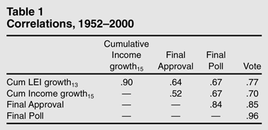
Table 1 shows bivariate correlations between the measure of leading economic indicator (LEI) growth and our final pre-election measures of income growth and approval as well as the final pre-election polls and the actual vote itself. The data relate to the 13 elections between 1952 and 2000. As for income growth, we measure LEI growth cumulatively during the current presidential term. Specifically, the measure is the weighted average of quarterly summaries of monthly growth, with each quarter weighted 0.90 as much as the following quarter (1.11 the weight of the preceding quarter). This weighting scheme maximizes the correlation with the presidential vote, which peaks using quarter 13 indicators, through the first quarter of the election year.6
The weight (.90) of prior quarterly information about LEI is greater than that (.80) for income growth, which implies greater discounting of the latter.
Measured in this way, cumulated leading indicators over a presidency represent the weighted accumulation of projected economic shocks, which smooth out as the aggregation of actual economic shocks. For additional detail about the measure, see the Appendix.
In Table 1 we can see that the quarter 13 measure of cumulative LEI growth nicely predicts the final, quarter 15 measure of cumulative income growth. The correlation is a healthy 0.90. The relationship partly reflects the strong correlation between the measure and quarterly income growth leading up to the election, especially in the 14th quarter of the cycle.7
The correlation is 0.88. The correlation with quarter 15 income growth is a much more modest 0.25.
It also reflects the fact that our measure of LEI summarizes income growth during the first 13 quarters, the correlation with which is 0.78. Notice as well in
Table 1 that leading indicators predict the final, pre-election reading of presidential approval from the Gallup poll. The correlation (0.64) is modest by comparison with what we see for income growth, which is as we would expect. That is, evaluations of sitting presidents reflect economics
and other things. Perhaps most importantly, LEI growth correlates well with the incumbent party share of the final pre-election poll and, even more so, the presidential vote.
8 These political variables measure the incumbent party share of the two-party vote, ignoring third party candidates such as Nader. The poll data are from Wlezien and Erikson (2002), and are available through the Inter-University Consortium for Political and Social Research (ICPSR): http://www.icpsr.org/.
Approval still is the better predictor: As we have noted, it captures other things besides economics and tells us quite a lot about what voters actually do. The polls tell most of all. Indeed, the correlation between the final preelection poll and the vote is a near-perfect 0.96. Taking into account sampling error, it is indistinguishable from unity. This is not surprising; it nevertheless is satisfying.
Now, let us see what the variables tell us when measured at different points in the election cycle, following our previous research (especially Wlezien and Erikson 1996). Our dependent variable is the incumbent party share of the two-party vote. The independent variables include the current quarterly readings of cumulative income growth and presidential approval during the election year.9
Except for the last quarter of the election cycle, the measure of approval is the average percentage of the public that approves of the president during each particular quarter or the most recent quarter for which data is available. The quarter 16 measure is the percentage of the public that approves of the president in October or the most recent month for which data is available.
We also include the quarter 13 measure of cumulative LEI growth.
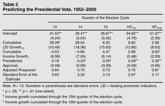
Table 2 shows the results of regression analysis for the final four quarters of the election cycle. These results are as expected given what we have already seen. The effect of LEI growth is greatest in the “quarter 13” model, using readings of income growth and approval through the first quarter of the election year. The effect drops off as more updated information about income growth and approval is used, which increasingly reflects the economic change predicted by early leading indicators. By the end of the cycle, the three variables, though particularly cumulative LEI and income growth, are highly correlated with each other.
This is especially true in the final pre-election models, in the third and fourth columns in Table 2. These models use a measure of income growth cumulated through quarter 15, which we know from Table 1 has a 0.90 correlation with the measure of quarter 13 cumulative LEI. The results in the fifth column indicate that income growth in the final quarter (substantially) helps predict the vote. Indeed, the quarter 16 measure of cumulative income growth clearly dominates the measure of LEI growth, and the increase in explained variance is significant (p<.01). The pattern implies that at least some portion of voters responds to the slope of the economy at the very end of the campaign. Regardless, the model is not useful for the purposes of forecasting, as quarter 16 data are not available until well after the election—specifically, not until the end of January, almost three months after the fact. Before the election, income growth adds absolutely nothing to our forecasting power (also see Wlezien and Erikson 1996).10
The coefficient for income growth in Table 2 actually is negative, though not statistically significant, in the quarter 13 and 14 models.
What about the 2004 election? Let us see what LEI growth and approval tell us now, at the end of the 14th quarter of this election cycle. To do so, we first estimate the following equation, excluding income growth:
where the subscripts 13 and 14 indicate the quarters of the election cycle and standard errors are in parentheses. Then, to produce a forecast for 2004, we simply plug the 2004 values of cumulative LEI growth and approval into the equation. Through the first quarter of 2004 (quarter 13 of the election cycle), the value of LEI growth is 0.195. The number is above average compared to the previous 13 election years (mean=0.14, s.d.=0.15).
11 However, it is virtually right in the middle, 7th highest of the 14. The median is .172.
This may surprise somewhat, as the economy did not perform well for Bush in his first three years. However, there were strong LEI gains in quarters 10–13, and these bode well for the election year economy. As for approval, Bush's most recent (June) number is 48%. Plugging this number and the LEI estimate into the equation predicts 52.8% of the two-party vote for Bush. Based on the model, therefore, it currently is advantage Bush. This advantage perhaps is best expressed as the probability of winning the majority share of the vote. We compute the
p-value using the forecast itself, the standard forecast error, and the
t distribution (with 10 degrees of freedom).
12 The standard error of the forecast takes into account the standard errors of the coefficients and thus is larger than the standard error of the estimate (also see Beck 2000).
Based on the statistical history of the model, we estimate Bush's chances at the moment to be a little better than 2/3.
The Fundamentals and the Polls
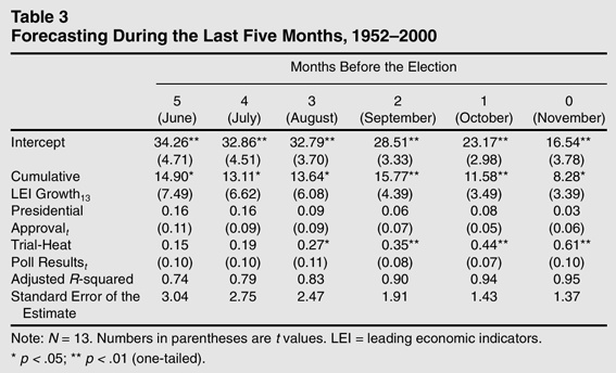
Not to be ignored is the information from trial-heat polls. As the campaign evolves and preferences develop, these polls become increasingly more informative about the outcome (Erikson and Wlezien 1996; Brown and Chappell 1999; Campbell 1996; 2000). Let us see what they add to our forecasting ability during the last five months of the campaign. Table 3 shows the regressions predicting the incumbent party vote from quarter 13 cumulative LEI growth, measures of approval and the incumbent candidate's poll share in each of the last five months prior to Election Day and at the very end of the cycle.13
As before, the approval data are from the Gallup poll and the poll results from Wlezien and Erikson (2002). For more details see note 8.
In the table we can see that the polls improve our forecasts quite a lot, though particularly as we move into the depths of summer, 3–4 months before the election. Early on, the polls are highly correlated (0.68) with presidential approval. Over the ensuing months, the correlation actually increases but the polls also incorporate other important information about the candidates. Thus, the size and significance of their effect on the vote increase markedly while the effect of presidential approval declines. The same is true for LEI growth, though note that the measure predicts the vote independently of the polls even in the final model. The result implies that the economy does not
fully register with voters until Election Day itself.
This analysis affords us another forecast for 2004. Recall from above that the value of quarter 13 cumulative LEI growth is .195 and that the president's June approval is 48%. The June trial-heat poll share is approximately 49% for Bush.14
This is based on polls from ABC/Washington Post, CBS/New York Times, and CNN/USA Today/Gallup. See www.pollingreport.com.
Inserting these numbers into the “5 months before” equation in the first column of
Table 3 predicts 52.2% of the vote for Bush. This is only slightly lower than we predicted without the polls, and is further evidence of a Bush advantage at this point in time. Indeed, the probability of victory remains about .67.
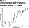
Of course, things can change leading up to the election. Indeed, it is from this point on that the polls become increasingly informative. This is clear in Figure 1, which displays the R-squareds (across the 13 election years) from regressing the vote division on quarter 13 cumulative LEI growth and the poll division for each date starting 200 days before the election, again using data from Wlezien and Erikson (2002). That is, we do exactly what we did in Table 3 except that we estimate a model using polling numbers for each day—instead of each month—and exclude approval, which allows us to isolate the effects of new poll information over time.15
Besides, approval does not add to our forecasting power during the final stages of the campaign, and decreasingly so as the cycle evolves (see Table 3).
Given that the measure of LEI growth does not change, the pattern of the
R-squareds from these 200 daily regressions tells us what the polls add from day to day.
Forecasting using Leading Economic Indicators and the Polls as the Election Campaign Unfolds, 1952–2000
In Figure 1 we can see that the model performs equally well using poll data from about 125–200 days before Election Day. There is a good amount of information at that point in time, as R-squareds hover between 70 and 75%. We see stark improvement in predictability thereafter, especially during the last 100 days of the campaign, and this improvement is essentially linear, with perhaps a slight hint of decreasing marginal returns. A ready interpretation is that the early campaign is largely frozen in place, but then picks up by midsummer— about the time the conventions occur—and continues through Election Day.16
For a more in-depth analysis, see Wlezien and Erikson (2002).
Regardless of the details, it is absolutely clear that the polls become more and more informative as the election campaign unfolds. This partly reflects the fact that polls increasingly reflect final Election Day judgments about the economy and the sitting president. They also reflect other aspects of preferences, some of which are not known or even knowable in advance. To the extent the latter is true, election forecasting is inherently dynamic.
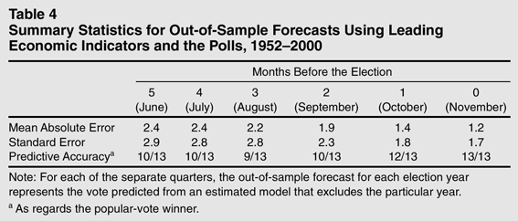
We can update our forecasts as we go along, using the additional information contained in the trial-heat polls. Table 4 reveals what happens when we simulate the past 13 elections. The table summarizes out-of-sample forecasts from a model containing the measure of cumulative LEI growth and the polls measured at monthly intervals. For each election, the out-of-sample forecast represents the vote predicted from an estimated model that excludes the particular year. Table 4 presents summary statistics of the “forecast” errors for each monthly model. Here we can see that the mean absolute out-of-sample forecast error is 2.4 percentage points using poll data from 4–5 months before the election. The mean error drops sharply when using poll data for the last three months, especially numbers from the fall general election campaign. By Election Day, the average absolute error is only 1.2 percentage points. The standard error shows a similar decline.
The third row of Table 4 summarizes the predictive accuracy of the out-of-sample forecasts in terms of the popular-vote winner. In this row we see that the accuracy remains largely unchanged using polls 2–5 months before Election Day. That is, we successfully forecast the winner in 10 (or 9) of the 13 elections during the period. Things really come into clear focus during the final 60 days. Using polls from 30 days out, the model correctly predicts 12 of the 13 winners. Using the final pre-election polls, the model correctly predicts all 13.
Conclusions
The foregoing analysis reveals the important impact of temporal horizons on election forecasting. Forecasts made at different points in time can differ meaningfully because of the available data. Well in advance of Election Day, the polls give us only a little insight about the final vote. Conditions in the country early on also provide only limited information about ultimate Election Day preferences. Even leading economic indicators do not perfectly predict how the economy will evolve in the coming months. We also cannot anticipate all new events that will affect the course of the campaign. The different effects on voters' preferences do become incorporated over time in the trial-heat polls, however, especially as Election Day approaches. This fact, while obvious, is important from the point of view of forecasting. Pre-election trial heats (increasingly) provide information about the “other things” that impact the ultimate vote.17
By the end of the campaign, the polls not only add to what we know about the economy and approval measured right before the election, they add to what we know about these variables after the election. Following the post-election model in the fifth column of Table 2, we first predicted the vote from quarter 13 LEI growth, the final pre-election reading of approval, and income growth cumulated through the 16th quarter. We then generated the predicted vote using this equation and estimated a vote equation containing this predicted vote variable and the final pre-election polls. From this analysis we see that the effect of the polls is statistically significant (b=.49; s.e.=.16) and the effect of the predicted vote (b=.40; s.e.=.20) actually is not. The same is true when either the presidential incumbency variable or Abramowitz's “time for a change” is included in the equation.
What then does this tell us about the 2004 election? As of this writing, five months in advance, the available information clearly is incomplete. We nevertheless can offer a tentative forecast. Our analysis of various combinations of economic conditions, leading indicators, presidential approval, and the latest polls themselves suggests a close race, with President Bush about a two-to-one favorite for reelection in November. Of course, to the extent past elections are any guide, this fuzzy prediction is subject to change.
We originally forecasted (on June 28) that Bush will receive 52.5% of the two-party presidential vote with a probability of election of about two-out-of-three. Given our modeling approach, we can update our forecasts as we go, virtually on a daily basis using new trial-heat polls. We update now, just in advance of the Republican convention, using the latest numbers available from pollingreport.com—specifically, the current Gallup presidential approval rating of 49% and the mean Bush two-party share in the four trial-heat polls reported in the last two weeks, which is 49.9%, a coin flip.18
We rely only on the results from samples of registered voters. The specific survey organizations are: CBS, CNN/USA Today/Gallup, Investor's Business Daily/Christian Science Monitor/TIPP, and the Los Angeles Times.
Our first model, containing the cumulative growth in leading economic indicators through quarter 13 and the August reading of presidential approval, predicts 52.9% for Bush, almost exactly what we predicted (52.8%) using the model estimated in June. Our second model, which adds in late-August trial-heat poll results, predicts only 51.7% for Bush. This is 1.2 percentage points lower than what we forecast without the trial-heats; it is 0.5 of a point lower than we forecasted two months earlier, using the corresponding June model. The implied probability of a Bush victory is about 75%.
Appendix: The Measure of Leading Economic Indicators
There are two different series of Leading Economic Indicators (LEI). The first—the one we traditionally have relied on—began in 1949 and ended in 1996. The second, newer series begins in 1959 and carries forward to the present. Beginning with this manuscript, we rely primarily on the newer, more updated, and presumably better series, available from The Conference Board. To preserve data for the years between 1952 and 1958, we use the original data as well. It was our original assumption that, although the series differed in levels and changes, percentage change measures would be comparable. Based on analysis of the overlapping years, however, we discovered that this was not true. It thus was necessary to predict the new LEI data from the old using the overlapping years. Let us outline the full details.
To begin with, we created the percentage change in the monthly leading economic indicators, i.e., (LEIt−LEIt−1)/LEIt−1*100. Notice that the numbers are not annualized. Next, we calculated the quarterly mean of these monthly numbers. For 1949–1958, we generated predicted quarterly numbers by simply regressing the new numbers on the old in the overlapping years, 1959–1996. Then we weight each quarter 0.90 as much as the following quarter (i.e., 1.11 the weight of the previous quarter), based on empirical analysis (Wlezien and Erikson 1996). Thus, LEI growth in quarter 13 counts approximately four times (1/.912) as much as LEI growth in the first quarter of the president's term. Finally, we sum the weighted quarterly growth rates through quarter 13 and then calculate the average. To calculate the average, we divide the sum of the weighted growth rates by the sum of the weights for the 13 quarters, not the number of quarters (13) itself. The sum of quarterly weights is 7.46. The resulting numbers are not that easy to interpret. For instance, the number (0.201) for 2000 indicates that the weighted average quarterly growth rate in monthly leading economic indicators is 0.201%. (To be absolutely clear, the weight is 1.0 in quarter 13, .9 in quarter 12, .81 in quarter 11, .729 in quarter 10, and so on to .912 in the first quarter of a presidential term.)
This article was presented at the Annual Meeting of the American Political Science Association, Chicago, September 2, 2004. We thank Cristina Adams, James Campbell, Mark Kayser, Des King, Pat Lynch, Iain McLean, Clive Payne, Laura Stoker, and Steve Yoder for comments on earlier incarnations.