1. Introduction
Current scientific, engineering and societal interest in the sequestration of
 $\text{CO}_{2}$
in underground brine-filled aquifers has motivated numerous recent studies of convection in porous media (Huppert & Neufeld Reference Huppert and Neufeld2014). The problem is complicated by uncertainties about the physical and chemical structure of the host rock and the intrinsic fluid-mechanical complexity of high-Rayleigh-number convection (Otero et al.
Reference Otero, Dontcheva, Johnston, Worthing, Kurganov, Petrova and Doering2004). The full chemical pathway of
 $\text{CO}_{2}$
dissolving in brine and reacting with host rock involves reaction rates spanning many orders of magnitude (Mitchell et al.
Reference Mitchell, Jensen, Cliffe and Maroto-Valer2010), while the large convective plumes arising in classical Rayleigh–Bénard porous-medium convection are intrinsically coupled to very thin boundary layers (Graham & Steen Reference Graham and Steen1994; Hewitt, Neufeld & Lister Reference Hewitt, Neufeld and Lister2012; Hidalgo et al.
Reference Hidalgo, Fe, Cueto-Felgueroso and Juanes2012; Slim Reference Slim2014). Computational simulations of the full reactive transport processes must therefore resolve very fine spatial and temporal features, restricting the parameter regimes that can be reliably investigated. There is significant benefit in deriving reliable low-order approximations of key underlying processes in order to facilitate the development of efficient multiscale simulations.
To this end we consider here an idealised problem involving a distributed source of solute at fixed concentration at the upper surface of a saturated porous medium. The solute dissolves in the interstitial liquid, raising its density and inducing gravity-driven convection. The solute simultaneously undergoes a first-order chemical reaction, interacting with the matrix of the porous medium, which limits the vertical penetration depth of the solute. At sufficiently high Rayleigh number
 $\mathit{Ra}$
(with molecular diffusion weak in comparison to convective flow, the regime appropriate to
 $\text{CO}_{2}$
sequestration applications (Ennis-King & Paterson Reference Ennis-King and Paterson2007)), the system can establish a statistically constant convective state, in which the net rate of supply of fresh solute is balanced by the net loss through chemical reaction. Our aim in this model problem is to quantify the net solute transfer rate at very high
 $\mathit{Ra}$
and understand how this is related to the structure of the convective flow; this extends our prior study of the two-dimensional flow close to the onset of convection (Ward et al.
Reference Ward, Cliffe, Jensen and Power2014). Inevitably, numerous features of real geological formations are neglected, notably changes in permeability and porosity due to dissolution or precipitation (Ritchie & Pritchard Reference Ritchie and Pritchard2011), depletion of the substrate during the reaction (Ghesmat, Hassanzadeh & Abedi Reference Ghesmat, Hassanzadeh and Abedi2009), heterogeneity and anisotropy of the host material (Rapaka et al.
Reference Rapaka, Pawar, Stauffer, Zhang and Chen2009; Bestehorn & Firoozabadi Reference Bestehorn and Firoozabadi2012), heterogeneity of the source (Szulczewski, Hesse & Juanes Reference Szulczewski, Hesse and Juanes2013) and three-dimensionality (Pau et al.
Reference Pau, Bell, Pruess, Almgren, Lijewski and Zhang2010; Fu, Cueto-Felgueroso & Juanes Reference Fu, Cueto-Felgueroso and Juanes2013; Hewitt, Neufeld & Lister Reference Hewitt, Neufeld and Lister2014). However, we anticipate that many of the processes and relationships revealed here will be relevant to flows involving these additional features.
Previous authors have modelled the reaction between dissolved
 $\text{CO}_{2}$
and minerals trapped in a fixed substrate as second-order (Ennis-King & Paterson Reference Ennis-King and Paterson2007; Ghesmat et al.
Reference Ghesmat, Hassanzadeh and Abedi2009). If the reaction rate is sufficiently rapid, the reaction is confined to a thin zone at the leading edge of the solute field (Ennis-King & Paterson Reference Ennis-King and Paterson2007). However, if the second-order reaction rate is slow compared to the convective time scale, and the solute is dilute in comparison to the substrate with which it reacts, the problem may instead be described using first-order reaction kinetics, at least over intermediate time scales (Ward et al.
Reference Ward, Cliffe, Jensen and Power2014). In this case the flow is parametrised by
 $\mathit{Ra}$
and a Damköhler number
 $\mathit{Da}$
(a dimensionless reaction rate). When the porous medium is shallow (or
 $\mathit{Da}$
is sufficiently small), the reaction can be further approximated as zeroth-order (Ward et al.
Reference Ward, Cliffe, Jensen and Power2014) and the problem parametrised by
 ${\it\gamma}=\mathit{Da}\,\mathit{Ra}^{2}$
. Alternatively, when the porous layer is sufficiently deep, the first-order system can be described by
 ${\it\beta}=\sqrt{Ra/Da}$
(Andres & Cardoso Reference Andres and Cardoso2011, Reference Andres and Cardoso2012; Ward et al.
Reference Ward, Cliffe, Jensen and Power2014). For fixed
 $\mathit{Da}$
, as
 $\mathit{Ra}$
increases from low values, the steady no-flow base state sequentially loses stability to eigenmodes with distinct patterns of convective rolls. These generate an intricate network of mixed-mode steady states in phase space, which provide a scaffold that is explored by the time-evolving flow (Ward et al.
Reference Ward, Cliffe, Jensen and Power2014).
The asymptotic structure of a non-reacting flow when
 $\mathit{Ra}$
becomes very large has been of long-standing interest in the context of two-sided thermal convection in a domain of fixed depth (Otero et al.
Reference Otero, Dontcheva, Johnston, Worthing, Kurganov, Petrova and Doering2004; Hewitt et al.
Reference Hewitt, Neufeld and Lister2012; Wen et al.
Reference Wen, Chini, Dianati and Doering2013). Here, thin boundary layers at the horizontal domain boundaries feed large vertical straight-sided columns filling the bulk of the flow domain. Most studies show that the time-averaged solute transfer rate, measured by a Sherwood or Nusselt number, increases proportionally to
 $\mathit{Ra}$
for sufficiently large
 $\mathit{Ra}$
. This is consistent with the notion that the solute transfer rate should be independent of molecular diffusivity at leading order, even though diffusion plays an intrinsic role in determining the structure of the columns (Hewitt, Neufeld & Lister Reference Hewitt, Neufeld and Lister2013b
; Slim Reference Slim2014). Previous authors have used a ‘heat-exchanger’ approximation to understand the columnar flow; Hewitt et al. (Reference Hewitt, Neufeld and Lister2013b
) provide evidence that wavenumber selection is determined via a stability criterion.
One-sided Rayleigh–Bénard–Darcy convection, with solute delivered just from the upper boundary, also exhibits a columnar structure, but is characterised by distinct temporal phases as the solute accumulates within the domain (Hewitt, Neufeld & Lister Reference Hewitt, Neufeld and Lister2013a ; Slim et al. Reference Slim, Bandi, Miller and Mahadevan2013; Slim Reference Slim2014). After introduction of the solute, a diffusive boundary layer becomes unstable to a fingering instability; the onset of convection has been intensively investigated, and a variety of techniques have been used to describe the growth of perturbations over a time-evolving base state (Riaz et al. Reference Riaz, Hesse, Tchelepi and Orr2006; Rapaka et al. Reference Rapaka, Chen, Pawar, Stauffer and Zhang2008; Rees, Selim & Ennis-King Reference Rees, Selim and Ennis-King2008; Daniel, Tilton & Riaz Reference Daniel, Tilton and Riaz2013; Myint & Firoozabadi Reference Myint and Firoozabadi2013; Tilton, Daniel & Riaz Reference Tilton, Daniel and Riaz2013; Tilton & Riaz Reference Tilton and Riaz2014). Once convection is fully established, but before plumes have grown sufficiently to interact with the base of the domain, the average rate of solute transfer is constant; the solute transfer rate begins to fall after the plumes reach the base of the box (Hewitt et al. Reference Hewitt, Neufeld and Lister2013a ; Slim Reference Slim2014).
Here we will assess the impact of a simple first-order chemical reaction on this configuration, focusing attention on the statistically constant convective state. The model we investigate is described in § 2 below. In § 3 we provide two-dimensional numerical realisations of the flow structure at high
 $\mathit{Ra}$
across a range of
 $\mathit{Da}$
, which we compare in §§ 4–6 to an approximate model that shows how a thin boundary layer near the upper surface feeds, and is sustained by upwelling fluid displaced by, slender plumes that penetrate into the porous medium. In particular, motivated by the work of Malkus (Reference Malkus1954) and Howard (Reference Howard and Görtler1964), who studied the Rayleigh–Bénard problem for pure fluid, we investigate the stability of an error-function-shaped time-averaged concentration boundary layer. In our case, small disturbances continually grow and are swept laterally by a forward-stagnation-point flow into a concentration hotspot where the dense fluid falls vertically under gravity. This basic structure persists in time, in contrast to Howard’s picture of the Rayleigh–Bénard problem, where Howard’s error function describes a time-dependent purely conductive state, which is disrupted by break-up into a thermal, before the diffusive boundary layer re-forms and the cycle is repeated. In the present problem, disturbances to the boundary layer grow within a restricted window of space and time and we employ a transient-growth analysis to track the growth of optimal perturbations. While similar approaches have been adopted to investigate the stability of spatially homogeneous time-evolving base states in porous-medium convection (Rapaka et al.
Reference Rapaka, Chen, Pawar, Stauffer and Zhang2008; Daniel et al.
Reference Daniel, Tilton and Riaz2013), here we investigate a spatially heterogeneous but steady base state. A marginal stability criterion turns out to be useful in establishing scalings for fully established convection and in explaining the growth of disturbances in the boundary layer but fails to specify flow parameters precisely. However, by coupling the boundary-layer analysis to a model for the underlying plumes, we provide a near-complete description of the convective state (the model reduces to four algebraic equations for five unknowns and is closed by extracting parameters from numerical simulations) and offer mechanistic insights into measured scaling relationships. We predict solute transfer rates for a wide range of
 $\mathit{Da}$
with
 $\mathit{Ra}\gg 1$
, finding when
 $\mathit{Da}$
is large an unexpected connection with the classical Rayleigh–Bénard–Darcy problem.
2. Model
We consider the dissolution of a solute in a two-dimensional homogeneous porous medium in which the solute undergoes a first-order A
 $\rightarrow$
B reaction, where species A (but not B) increases the solution density and the substrate of the reaction remains abundant (Ward et al.
Reference Ward, Cliffe, Jensen and Power2014). The non-dimensionalised equations governing the system are the continuity equation (which is eliminated by introducing a streamfunction), the convection–diffusion–reaction equation and Darcy’s law,
 $$\begin{eqnarray}C_{t^{\ast }}^{\ast }+{\it\psi}_{z^{\ast }}^{\ast }C_{x^{\ast }}^{\ast }-{\it\psi}_{x^{\ast }}^{\ast }C_{z^{\ast }}^{\ast }=\frac{1}{\mathit{Ra}}(C_{x^{\ast }x^{\ast }}^{\ast }+C_{z^{\ast }z^{\ast }}^{\ast })-\mathit{Da}\,C^{\ast },\quad {\it\psi}_{x^{\ast }x^{\ast }}^{\ast }+{\it\psi}_{z^{\ast }z^{\ast }}^{\ast }=-C_{x^{\ast }}^{\ast },\end{eqnarray}$$
defined on the domain
 $z^{\ast }\in [-1,1]$
,
 $x^{\ast }\in [0,\mathscr{L}]$
; gravity acts in the direction of increasing
 $z^{\ast }$
. The boundary conditions are
 $$\begin{eqnarray}\displaystyle C^{\ast }(x^{\ast },-1,t^{\ast })=1, & \quad & \displaystyle C_{z^{\ast }}^{\ast }(x^{\ast },1,t^{\ast })=0,\end{eqnarray}$$
 $$\begin{eqnarray}\displaystyle {\it\psi}^{\ast }(x^{\ast },-1,t^{\ast })=0, & \quad & \displaystyle {\it\psi}^{\ast }(x^{\ast },1,t^{\ast })=0,\end{eqnarray}$$
 $$\begin{eqnarray}\displaystyle C^{\ast }(x^{\ast },z^{\ast },t^{\ast })=C^{\ast }(x^{\ast }+\mathscr{L},z^{\ast },t^{\ast }), & \quad & \displaystyle {\it\psi}^{\ast }(x^{\ast },z^{\ast },t^{\ast })={\it\psi}^{\ast }(x^{\ast }+\mathscr{L},z^{\ast },t^{\ast }).\end{eqnarray}$$
 $C^{\ast }$
and
 ${\it\psi}^{\ast }$
are the non-dimensional concentration of species A and the streamfunction, respectively. In (2.2),
 $C^{\ast }$
is held constant at the upper boundary of the domain and no-flux conditions apply at its base; periodic conditions are applied on the lateral boundaries. Dimensional variables are defined as
 $(\hat{x}^{\ast },\hat{z}^{\ast })=H(x^{\ast },z^{\ast })$
,
 $\hat{t}^{\ast }=(H{\it\varphi}{\it\mu})t^{\ast }/({\it\delta}Kg\mathscr{C})$
,
 ${\hat{C}}^{\ast }=\mathscr{C}C^{\ast }$
and
 $\hat{{\it\psi}}^{\ast }=(KgH\mathscr{C}{\it\delta}){\it\psi}^{\ast }/{\it\mu}$
. The Rayleigh number,
 $\mathit{Ra}$
, and the Damköhler number,
 $\mathit{Da}$
, characterising the size of the diffusive and uptake terms in (2.1), are defined by
 $$\begin{eqnarray}\mathit{Ra}=\frac{HKg\mathscr{C}{\it\delta}}{{\it\varphi}{\it\mu}D},\quad \mathit{Da}=\frac{{\it\alpha}{\it\varphi}H{\it\mu}}{Kg\mathscr{C}{\it\delta}},\end{eqnarray}$$
where
 $2H$
,
 $K$
,
 ${\it\mu}$
,
 $D$
,
 ${\it\varphi}$
,
 ${\it\alpha}$
,
 $g$
,
 ${\it\delta}$
and
 $\mathscr{C}$
are the dimensional domain depth, medium permeability, solvent viscosity, solute diffusion coefficient, medium porosity, solute reaction rate, acceleration due to gravity, density increase per unit concentration of solute and the dimensional solute concentration. Here,
 $\mathit{Ra}$
and
 $\mathit{Da}$
are defined in terms of the domain half-depth, making them half the value reported in some other studies.
The net uptake of solute (in units of
 $\mathscr{C}{\it\varphi}D/H$
) is expressed using the Sherwood number,
 $$\begin{eqnarray}\mathit{Sh}^{\ast }(t^{\ast };\mathit{Ra},\mathit{Da})=\langle -C_{z^{\ast }}^{\ast }(x^{\ast },-1,t^{\ast })\rangle ,\quad \text{where}\ \langle \,\cdot \,\rangle \equiv \frac{1}{\mathscr{L}}\int _{0}^{\mathscr{L}}\cdot \,\text{d}\mathit{x}^{\ast },\end{eqnarray}$$
and, when the system is in a statistically constant state, by its time average,
 $\overline{\mathit{Sh}^{\ast }}(\mathit{Ra},\mathit{Da})$
. Integration of (2.1) subject to (2.2) shows that the total dimensionless mass
 $M^{\ast }$
(in units of
 $\mathscr{C}{\it\varphi}H^{2}$
) of dissolved solute satisfies
 $$\begin{eqnarray}M_{t^{\ast }}^{\ast }=(\mathscr{L}\mathit{Sh}^{\ast }/\mathit{Ra})-\mathit{Da}\,M^{\ast }\quad \text{where}\ M^{\ast }(t^{\ast })\equiv \int _{0}^{\mathscr{L}}\!\int _{-1}^{1}C^{\ast }\text{d}z^{\ast }\text{d}x^{\ast }.\end{eqnarray}$$
Note that superscripts
 $\text{}^{\ast }$
and
 $\text{}^{\star }$
are used for this general formulation and for the intermediate case
 $\mathit{Da}=O(1)$
, respectively.
For
 $\mathit{Ra}\,Da\gg 1$
, strong solute uptake confines the distribution to a region close to the upper boundary and the domain depth has negligible influence on the convection (Andres & Cardoso Reference Andres and Cardoso2011, Reference Andres and Cardoso2012; Ward et al.
Reference Ward, Cliffe, Jensen and Power2014). In this limit we introduce the associated leading-order deep-domain problem with depth-independent parameters
 $$\begin{eqnarray}{\it\beta}^{2}=\mathit{Ra}/\mathit{Da},\quad {\it\Lambda}=\sqrt{\mathit{Ra }\,\mathit{Da}}\,\mathscr{L},\end{eqnarray}$$
and new variables
 $(x,z)=\sqrt{\mathit{Ra }\,\mathit{Da}}(x^{\ast },(z^{\ast }+1))$
,
 $C={\it\beta}C^{\ast }$
,
 $t=t^{\ast }\mathit{Ra}/{\it\beta}^{2}$
and
 ${\it\psi}={\it\beta}\sqrt{\mathit{Ra }\,\mathit{Da}}\,{\it\psi}^{\ast }$
. Equations (2.1) and (2.2) then become, in the limit
 $\mathit{Ra}\,\mathit{Da}\rightarrow \infty$
with
 ${\it\beta}=O(1)$
,
 $$\begin{eqnarray}C_{t}+{\it\psi}_{z}C_{x}-{\it\psi}_{x}C_{z}=C_{xx}+C_{zz}-C,\quad {\it\psi}_{xx}+{\it\psi}_{zz}=-C_{x},\end{eqnarray}$$
subject to
 $$\begin{eqnarray}\displaystyle C(x,0,t)={\it\beta}, & \quad & \displaystyle C_{z}\rightarrow 0\quad \text{as}\ z\rightarrow \infty ,\end{eqnarray}$$
 $$\begin{eqnarray}\displaystyle {\it\psi}(x,0,t)=0, & \quad & \displaystyle {\it\psi}\rightarrow 0\quad \text{as}\ z\rightarrow \infty ,\end{eqnarray}$$
 $$\begin{eqnarray}\displaystyle C(x,z,t)=C(x+{\it\Lambda},z,t), & \quad & \displaystyle {\it\psi}(x,z,t)={\it\psi}(x+{\it\Lambda},z,t).\end{eqnarray}$$
 $$\begin{eqnarray}\mathit{Sh}(t;{\it\beta})=\langle -C_{z}(x,0,t)\rangle\end{eqnarray}$$
(integrating over
 $(0,{\it\Lambda})$
), where
 $\mathit{Sh}^{\ast }=\mathit{Sh}\,\mathit{Da}$
; the mass of dissolved solute,
 $M(t)\equiv \int _{0}^{{\it\Lambda}}\!\int _{0}^{\infty }C\,\text{d}z\,\text{d}x$
, satisfies
 $M_{t}={\it\Lambda}\,\mathit{Sh}-M$
. Note that variables without superscripts are used in the deep-domain case.
Alternatively, for
 $\mathit{Ra}\,\mathit{Da}\ll 1$
, solute diffuses quickly across the domain and we introduce the associated shallow-domain problem (Ward et al.
Reference Ward, Cliffe, Jensen and Power2014) with parameter
 $$\begin{eqnarray}{\it\gamma}=\mathit{Da}\,\mathit{Ra}^{2},\end{eqnarray}$$
and new variables
 $C^{\ast }=1+\mathit{Ra}\,\mathit{Da}\,C^{\prime }$
,
 ${\it\psi}^{\ast }=\mathit{Ra}\,\mathit{Da}\,{\it\psi}^{\prime }$
,
 $(x^{\ast },z^{\ast })=(x^{\prime },z^{\prime })$
and
 $t^{\ast }=\mathit{Ra}\,t^{\prime }$
, so that (2.1) and (2.2) become, in the limit
 $\mathit{Ra}\,\mathit{Da}\rightarrow 0$
with
 ${\it\gamma}=O(1)$
,
 $$\begin{eqnarray}C_{t^{\prime }}^{\prime }+{\it\gamma}({\it\psi}_{z^{\prime }}^{\prime }C_{x^{\prime }}^{\prime }-{\it\psi}_{x^{\prime }}^{\prime }C_{z^{\prime }}^{\prime })=C_{x^{\prime }x^{\prime }}^{\prime }+C_{z^{\prime }z^{\prime }}^{\prime }-1,\quad {\it\psi}_{x^{\prime }x^{\prime }}^{\prime }+{\it\psi}_{z^{\prime }z^{\prime }}^{\prime }=-C_{x^{\prime }}^{\prime },\end{eqnarray}$$
subject to
 $$\begin{eqnarray}\displaystyle C^{\prime }(x^{\prime },-1,t^{\prime })=0, & \quad & \displaystyle C_{z^{\prime }}^{\prime }(x^{\prime },1,t^{\prime })=0,\end{eqnarray}$$
 $$\begin{eqnarray}\displaystyle {\it\psi}^{\prime }(x^{\prime },-1,t^{\prime })=0, & \quad & \displaystyle {\it\psi}^{\prime }(x^{\prime },1,t^{\prime })=0,\end{eqnarray}$$
 $$\begin{eqnarray}\displaystyle C^{\prime }(x^{\prime },z^{\prime },t^{\prime })=C^{\prime }(x^{\prime }+\mathscr{L},z^{\prime },t^{\prime }), & \quad & \displaystyle {\it\psi}^{\prime }(x^{\prime },z^{\prime },t^{\prime })={\it\psi}^{\prime }(x^{\prime }+\mathscr{L},z^{\prime },t^{\prime }).\end{eqnarray}$$
 $$\begin{eqnarray}\mathit{Sh}^{\prime }(t^{\prime };{\it\gamma})=\langle -C_{z^{\prime }}^{\prime }(x^{\prime },-1,t^{\prime })\rangle ,\end{eqnarray}$$
where
 $\mathit{Sh}^{\ast }=\mathit{Ra}\,\mathit{Da}\,\mathit{Sh}^{\prime }$
. The mass of dissolved solute,
 $M^{\prime }(t^{\prime })\equiv \int _{0}^{\mathscr{L}}\!\int _{-1}^{1}C^{\prime }\text{d}z^{\prime }\text{d}x^{\prime }$
, satisfies
 $M_{t^{\prime }}^{\prime }=\mathscr{L}(\mathit{Sh}^{\prime }-2)$
, implying that the time-averaged flux in this shallow-domain problem satisfies
 $$\begin{eqnarray}\overline{\mathit{Sh}^{\prime }}=2.\end{eqnarray}$$
In this case, the leading-order uptake rate (dimensionally, it is
 $2\mathscr{C}{\it\phi}{\it\alpha}H$
,
 $2H$
being the depth of the domain) is restricted by the depth of the domain. This approximation does not capture initial transients that may arise when the solute concentration
 $C^{\ast }$
in the bulk differs significantly from unity. Note that primed variables are used in the shallow-domain case.
As shown in Ward et al. (Reference Ward, Cliffe, Jensen and Power2014), the pure-conduction state of (2.1) and (2.2),
 $$\begin{eqnarray}C^{\ast }=\frac{\cosh (\sqrt{\mathit{Ra }\,\mathit{Da}}(1-z^{\ast }))}{\cosh (2\sqrt{\mathit{Ra }\,\mathit{Da}})},\quad {\it\psi}^{\ast }=0,\quad \mathit{Sh}^{\ast }=\sqrt{\mathit{Ra }\,\mathit{Da}}\tanh (2\sqrt{\mathit{Ra }\,\mathit{Da}}),\end{eqnarray}$$
is linearly unstable to perturbations for
 $\mathit{Ra}>\mathit{Ra}_{c}(\mathit{Da})$
, where
 $\mathit{Ra}_{c}(\mathit{Da})$
is plotted in figure 1. For
 $\mathit{Da}\gg 1$
,
 $\mathit{Ra}_{c}\approx \mathit{Da}{\it\beta}_{c}^{2}$
where
 ${\it\beta}_{c}\approx 19.9$
; for
 $\mathit{Da}\ll 1$
,
 $\mathit{Ra}_{c}\approx ({\it\gamma}_{c}/\mathit{Da})^{1/2}$
for
 ${\it\gamma}_{c}\approx 7.73$
. Below, we will address solutions of (2.1) and (2.2) for
 $\mathit{Ra}\gg 1$
with
 $\mathit{Da}=O(1)$
, and show how these connect to solutions of (2.7) and (2.8) for
 ${\it\beta}\gg 1$
(with
 $1\ll \mathit{Da}\ll Ra$
) and (2.11) and (2.12) with
 ${\it\gamma}\gg 1$
(with
 $\mathit{Ra}^{-2}\ll \mathit{Da}\ll 1$
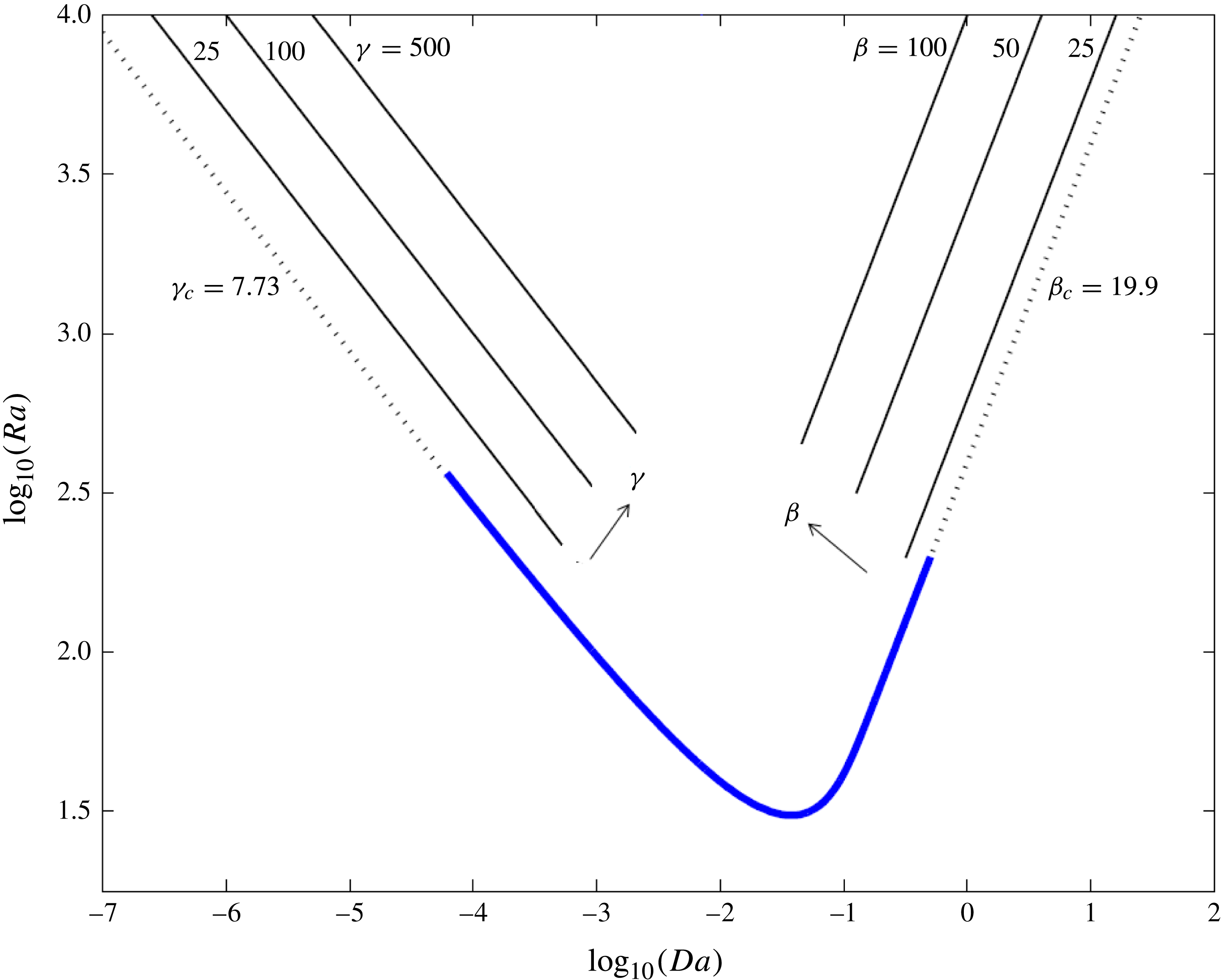
). As figure 1 suggests, this provides comprehensive coverage of parameter space.
The linear stability envelope
 $\mathit{Ra}_{c}(\mathit{Da})$
(thick solid curve; blue online) in
 $(\mathit{Ra},\mathit{Da})$
parameter space, below which the no-flow state (2.15) is stable. Dashed lines show asymptotic approximations for
 $\mathit{Da}\ll 1$
and
 $\mathit{Da}\gg 1$
with
 ${\it\gamma}_{c}\approx 7.73$
and
 ${\it\beta}_{c}\approx 19.9$
, respectively. Straight lines illustrate the effect of increasing the parameters
 ${\it\gamma}$
and
 ${\it\beta}$
.

For fully developed convection in the limit
 $\mathit{Ra}\gg 1$
, it is reasonable to expect the leading-order dimensional uptake rate to be independent of molecular diffusivity. Thus on dimensional grounds, for
 $\mathit{Da}=O(1)$
, we expect
 $\overline{\mathit{Sh}^{\ast }}(\mathit{Ra},\mathit{Da})\sim \mathit{Ra}\,\overline{\mathit{Sh}_{0}^{\ast }}(\mathit{Da})$
for
 $\mathit{Ra}\gg 1$
and some function
 $\overline{\mathit{Sh}_{0}^{\ast }}(\mathit{Da})$
, which measures uptake rate in units of
 $\mathscr{C}^{2}Kg{\it\delta}/{\it\mu}$
. Likewise, for large
 $\mathit{Da}$
(corresponding to the limit
 ${\it\beta}\gg 1$
), we anticipate that
 $\overline{\mathit{Sh}}({\it\beta})\sim {\it\beta}^{2}\,\overline{\mathit{Sh}_{0}}$
for some constant
 $\overline{\mathit{Sh}_{0}}$
(which is equivalent to
 $\overline{\mathit{Sh}_{0}^{\ast }}(\mathit{Da})\rightarrow \overline{\mathit{Sh}_{0}}$
for
 $1\ll \mathit{Da}$
). The condition (2.14) requires
 $\overline{\mathit{Sh}_{0}^{\ast }}(\mathit{Da})\sim 2\mathit{Da}$
for
 $\mathit{Da}\ll 1$
.
Equations (2.1)–(2.2), (2.7)–(2.8) and (2.11)–(2.12) were solved numerically using a spectral method, the details of which are given in appendix A. Quantities such as the time- and horizontally averaged concentration,
 $\overline{\langle C\rangle }(z)$
, were calculated over a time interval
 $(T_{0},T_{0}+T)$
in which solutions to (2.1) and (2.2) had reached a statistically constant state that was independent of the initial condition. Starting from either a perturbed no-flow steady solution or an unsteady solution at nearby parameter values,
 $T_{0}$
was selected as the time at which the rate of change of
 $M^{\ast }$
(or
 $M$
and
 $M^{\prime }$
) was sufficiently close to zero. The time interval
 $T$
was chosen to ensure that relative changes of estimates of
 $\overline{\mathit{Sh}^{\ast }}$
were less than
 $10^{-6}$
.
3. Numerical simulations of high-
 $\mathit{Ra}$
convection

We begin by addressing the simpler deep-domain and shallow-domain problems before reporting results for the full two-parameter problem.
3.1. Deep-domain limit:
${\it\beta}\gg 1$
,
$1\ll \mathit{Da}\ll \mathit{Ra}$


When
 $\mathit{Da}\gg 1$
, the time scale for reaction is much shorter than the time taken for the solute to diffuse across the domain. This maintains a small penetration depth of solute; the system is described by (2.7) and (2.8) and the depth-independent parameters
 ${\it\beta}=(\mathit{Ra}/\mathit{Da})^{1/2}$
and
 ${\it\Lambda}=(\mathit{Ra}\,\mathit{Da})^{1/2}\mathscr{L}$
. For
 ${\it\beta}<{\it\beta}_{c}\approx 19.9$
, the system is linearly stable and the concentration of solute is given by the horizontally uniform base state
 $C_{0}(z)\approx {\it\beta}\exp (-z)$
,
 ${\it\psi}_{0}=0$
. Disordered time-dependent behaviour arises for
 ${\it\beta}>{\it\beta}_{c}$
, as an increasing number of eigenmodes lose stability (Ward et al.
Reference Ward, Cliffe, Jensen and Power2014). Figure 1 illustrates how, for sufficiently large
 $\mathit{Da}$
, solutions of (2.7) and (2.8) for fixed
 ${\it\beta}$
correspond to a family of solutions to (2.1) and (2.2) for which
 $\mathit{Ra}/\mathit{Da}={\it\beta}^{2}$
; thus increasing
 ${\it\beta}$
corresponds to increasing
 $\mathit{Ra}$
for fixed
 $\mathit{Da}$
or decreasing
 $\mathit{Da}$
for fixed
 $\mathit{Ra}$
.
Simulations of (2.7) and (2.8) for
 ${\it\beta}\gg 1$
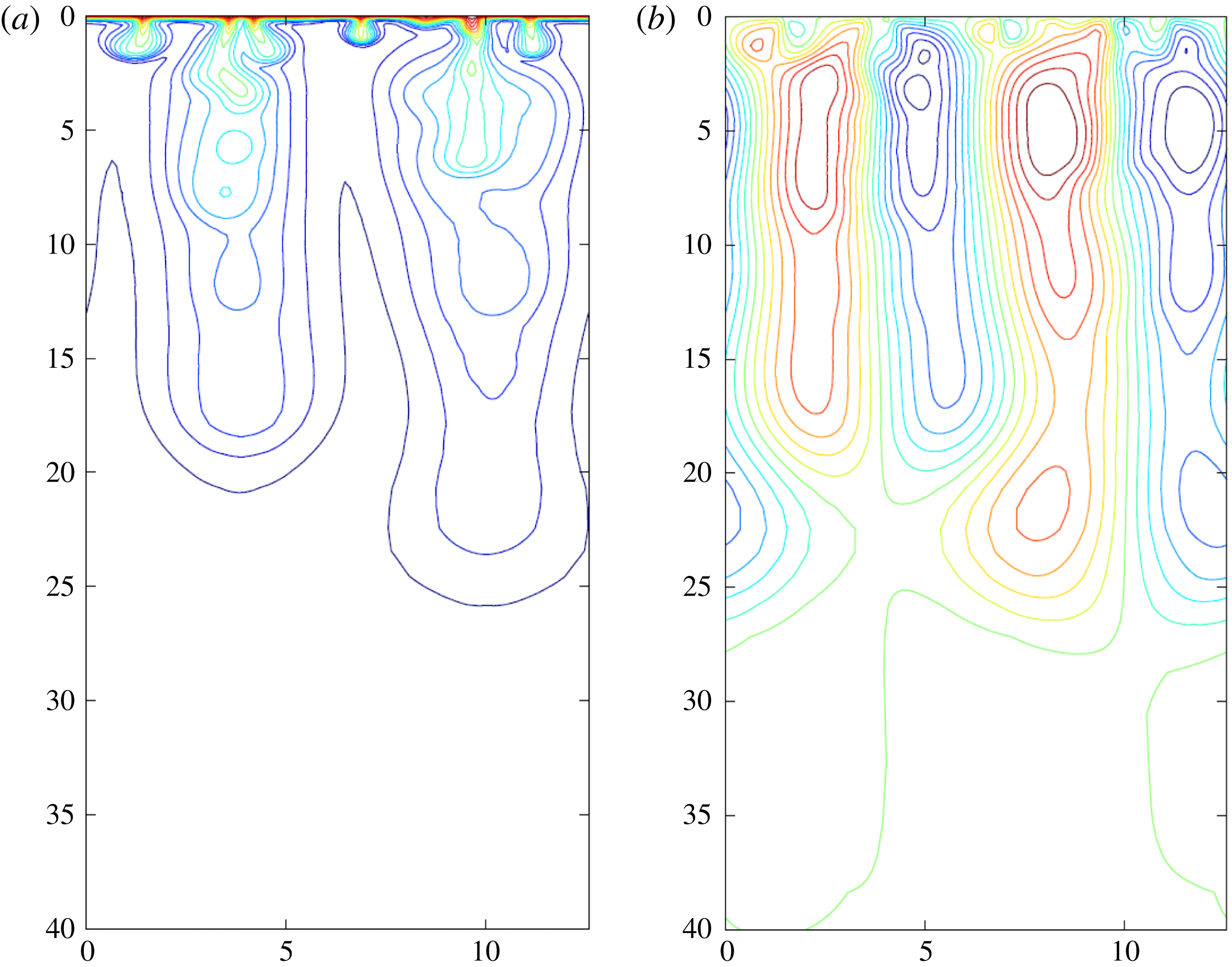
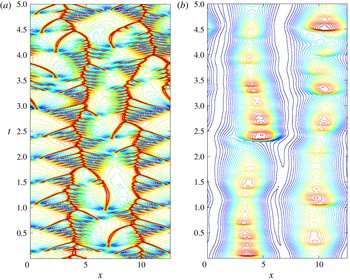
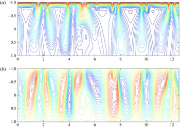
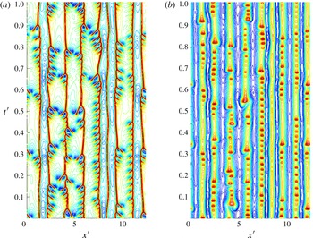
reveal how at large times an active boundary layer forms near the upper surface and large plumes sink into the domain below (see figure 2 and the supplementary movie available at http://dx.doi.org/10.1017/jfm.2014.594). The large plumes transport solute away from the boundary; the solute concentration decays as it descends, but creates an upwelling of dilute solvent between the plumes. Small plumes also form in the boundary layer and grow before being swept horizontally across the boundary layer, driven by the recirculation of the dilute solvent towards a concentration ‘hotspot’. This acts as a negative-buoyancy source for larger plumes to grow deeper into the domain. The supplementary movie illustrates the rich dynamics of the interacting plumes and boundary layer. To illustrate the evolution over longer times, figure 3 shows horizontal slices (for fixed
 $z$
) of the concentration field, presented as space–time maps for
 ${\it\beta}=200$
. Figure 3(a) resembles a fishbone pattern where the two tracks running vertically (the ‘backbones’) correspond to the concentration hotspots forming the centre of two large plumes, and the shorter horizontal tracks (the ‘ribs’) represent smaller plumes forming in the boundary layer and being swept towards the concentration hotspots. Similar patterns have been reported by Hewitt et al. (Reference Hewitt, Neufeld and Lister2012) and Slim (Reference Slim2014). Each backbone shows distinct kinks where it merges with larger ribs, indicating interactions between small plumes and concentration hotspots. Once the smaller plumes are absorbed by a concentration hotspot, there can be transient increases in solute concentration in the larger plumes, as pulses of denser fluid sink intermittently to the bottom of the plume (figure 3
b).


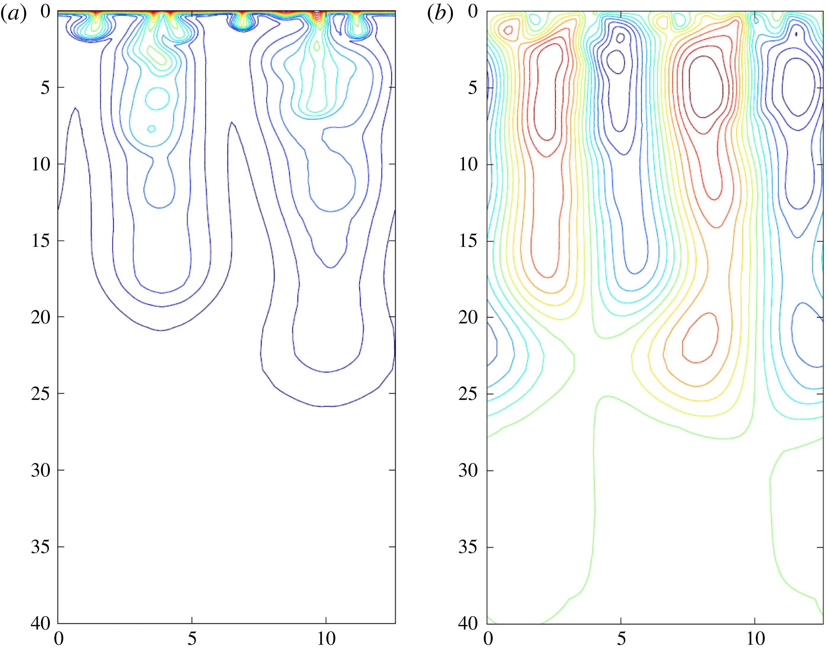
Space–time maps of the concentration field for
 ${\it\beta}=200$
,
 ${\it\Lambda}=4{\rm\pi}$
evaluated at (a)
 $z=0.1$
(within the boundary layer) and (b)
 $z=12.5$
(cutting across large vertical plumes). Pulses in panel (b) can be traced to mergers of smaller plumes within the boundary layer (panel (a)) approximately 0.5 time units earlier.

For larger
 ${\it\beta}$
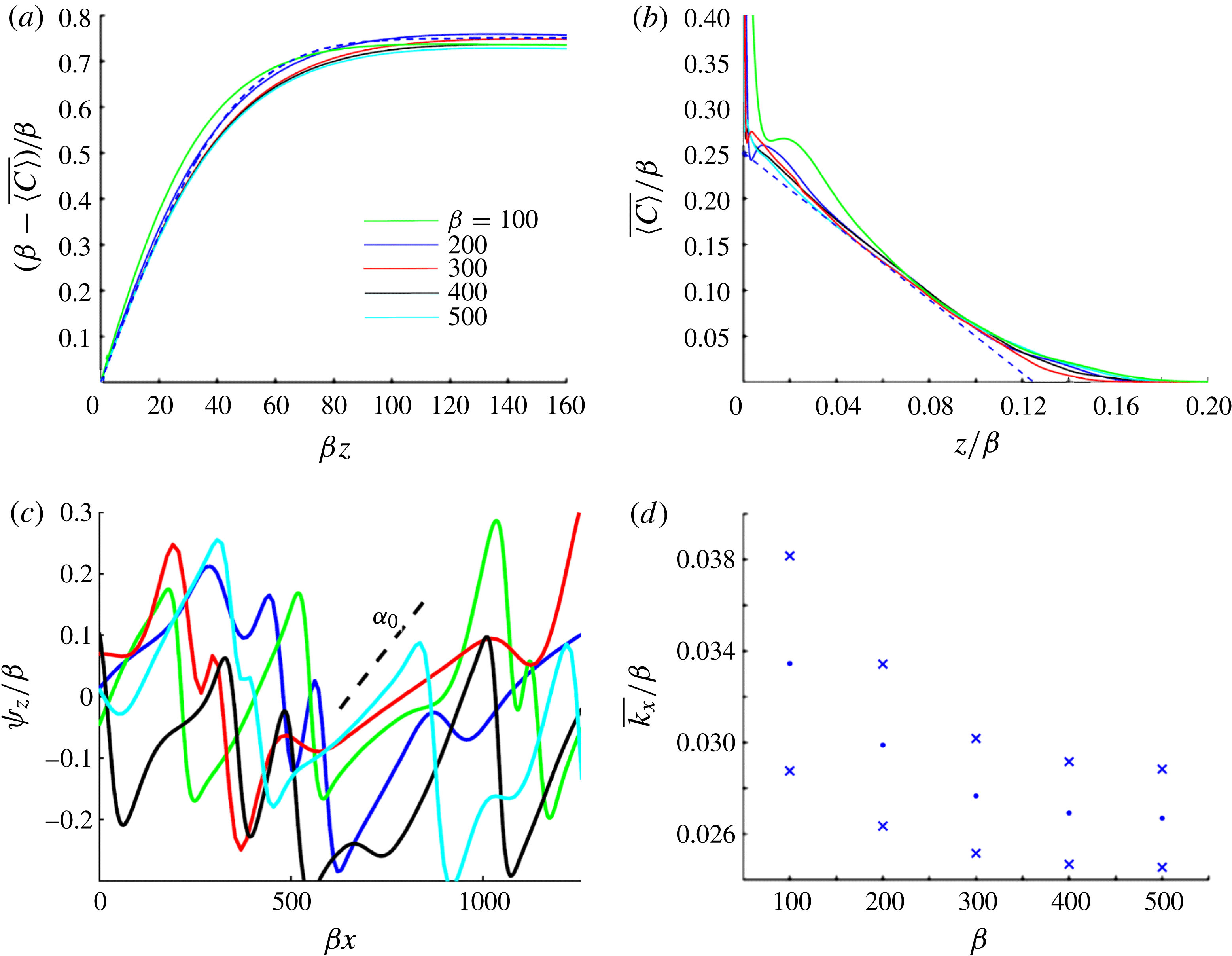
, the boundary layer becomes increasingly disordered, with small plumes forming and being swept into the concentration hotspots at a faster rate. Time- and horizontally averaged concentration profiles are fitted well by an error function in the boundary layer, over which the concentration falls abruptly (figure 4
a), before decaying approximately linearly deeper in the domain (figure 4
b). Collapse of the solutions for different values of
 ${\it\beta}$
in figure 4 suggests that the penetration depth of the boundary layer is
 $O(1/{\it\beta})$
and the penetration depth of the larger plumes is
 $O({\it\beta})$
. These scalings are supported by analysis in § 4 below. We expect the boundary layer to be sufficiently thin for the reaction of solute to have negligible influence in this region. The time-averaged vertical solute flux switches from being purely diffusive at
 $z=0$
(where
 ${\it\psi}_{x}=0$
) to fully advective at the outer edge of the boundary layer (where
 $\overline{\langle C\rangle }_{z}\approx 0$
).
Profiles of the time- and horizontally averaged concentration field
 $\overline{\langle C\rangle }$
plotted against (a)
 ${\it\beta}z$
and (b)
 $z/{\it\beta}$
for
 ${\it\Lambda}=4{\rm\pi}$
and
 ${\it\beta}$
values as shown. For later reference, the error function approximation (4.2) (dashed) in § 4 is plotted in panel (a) with
 ${\it\alpha}={\it\alpha}_{0}{\it\beta}^{2}$
,
 ${\it\alpha}_{0}=8\times 10^{-4}$
and
 ${\it\lambda}=0.25$
. The approximation
 $C/{\it\beta}={\it\lambda}(1-z/z_{0})$
with
 $z_{0}={\it\zeta}{\it\beta}$
and
 ${\it\zeta}=0.125$
(dashed) is plotted in panel (b). (c) Snapshots of the horizontal velocity along
 $z=0$
for the given
 ${\it\beta}$
values: although highly variable, the magnitude of the mean velocity is of order
 ${\it\beta}$
; strain rates are comparable in magnitude to
 ${\it\alpha}={\it\alpha}_{0}{\it\beta}^{2}$
(as indicated by the dashed line) where the flow is elongating above an upwelling (
 ${\it\psi}_{xz}>0$
), and even larger where the surface flow is compressive (
 ${\it\psi}_{xz}<0$
). (d) Time-averaged wavenumber of plumes in the boundary layer (dots) evaluated at
 $z=10/{\it\beta}$
; the crosses represent
 $\pm$
one standard deviation.

Figure 4(c) shows snapshots of the horizontal velocity along
 $z=0$
. Instantaneously, the surface velocity has regions of rapid stretching (
 ${\it\psi}_{xz}>0$
) interspersed by short regions of even greater compression (
 ${\it\psi}_{xz}<0$
), which correspond to the bases of plumes descending from the boundary layer. As suggested by figure 3, the surface velocity profile is very dynamic, as plumes continually migrate and merge.
We estimate the horizontal wavenumber in the boundary layer following Slim (Reference Slim2014) by defining
 ${\hat{C}}=C-\langle C\rangle$
and computing the time average
 $\overline{k_{x}}$
and variance of
 $$\begin{eqnarray}k_{x}=\sqrt{\langle {\hat{C}}_{x}^{2}\rangle /\langle {\hat{C}}^{2}\rangle }.\end{eqnarray}$$
Figure 4(d) suggests that, for large
 ${\it\beta}$
, plumes in the boundary layer have a wavelength that scales with the boundary-layer depth
 $1/{\it\beta}$
.
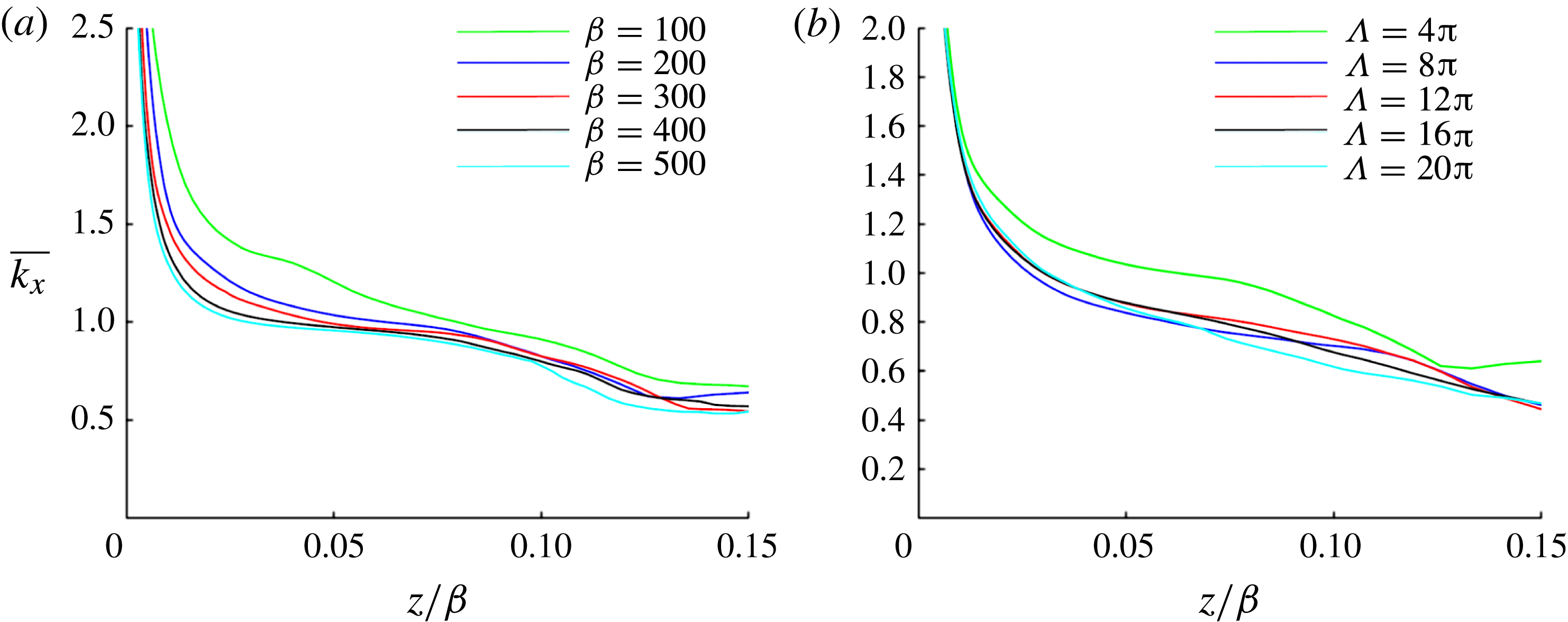
To characterise the structure of the large plumes beneath, figure 5 shows the time-averaged horizontal wavenumber calculated using (3.1). Using this measure of the wavenumber,
 $\overline{k_{x}}$
varies with depth, albeit weakly sufficiently below the boundary layer. Figure 5(a) shows that the dominant wavenumber does not vary appreciably with
 ${\it\beta}$
, at least over the range of
 ${\it\beta}$
investigated, nor with the width
 ${\it\Lambda}$
of the box (figure 5
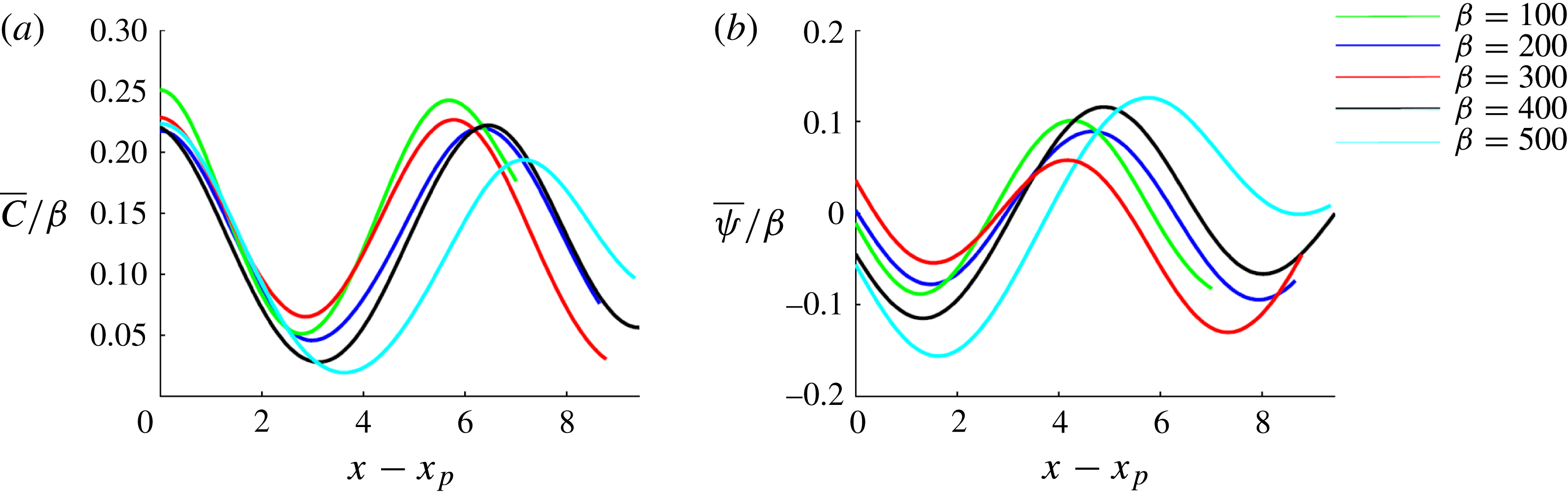
b). Figure 6 shows horizontal slices of the time-averaged concentration field and streamfunction (measured from the centre of a large plume), suggesting that the large plumes have a sinusoidal structure in the
 $x$
direction.
Wavenumber of the large plumes calculated using (3.1) for (a)
 ${\it\beta}=100$
, 200, 300, 400, 500,
 ${\it\Lambda}=4{\rm\pi}$
and (b)
 ${\it\Lambda}=4{\rm\pi},8{\rm\pi},12{\rm\pi},16{\rm\pi},20{\rm\pi}$
,
 ${\it\beta}=200$
.

(a) Concentration and (b) streamfunction profiles taken at
 $z={\it\zeta}{\it\beta}/2$
,
 ${\it\zeta}=0.125$
, obtained from time-averaged data for
 ${\it\Lambda}=4{\rm\pi}$
,
 ${\it\beta}=100,200,300,400$
and 500. Profiles are plotted against a shifted
 $x$
coordinate, where
 $x_{p}$
is the centre of a plume.

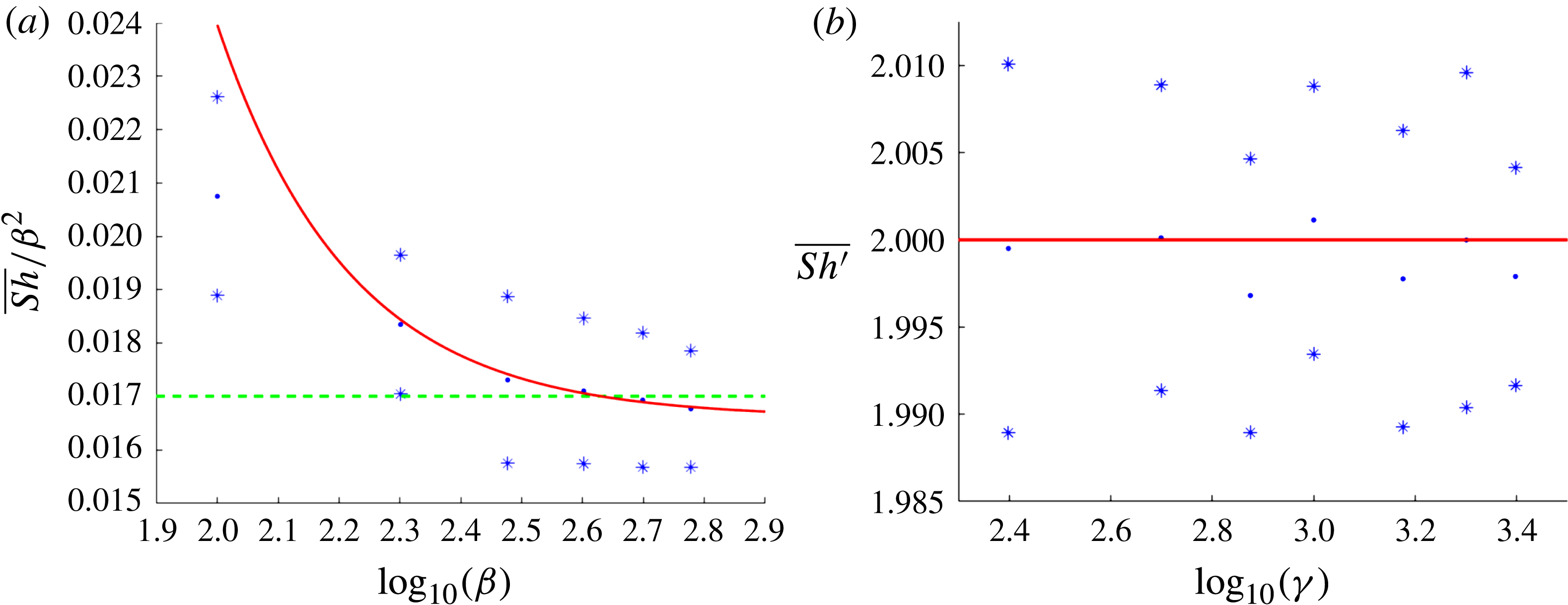
Figure 7(a) shows the time-averaged uptake rate
 $\overline{\mathit{Sh}}/{\it\beta}^{2}$
for
 ${\it\beta}\gg 1$
. The data support the conjecture that
 $\overline{\mathit{Sh}}$
scales like
 ${\it\beta}^{2}$
for
 ${\it\beta}\gg 1$
(at least for the range of
 ${\it\beta}$
investigated; equivalently, that
 $\overline{\mathit{Sh}^{\ast }}$
scales like
 $\mathit{Ra}$
for
 $1\ll \mathit{Da}\ll \mathit{Ra}$
). Furthermore,
 $\overline{\mathit{Sh}}/{\it\beta}^{2}$
fluctuates around 0.017, the mean dimensionless solute flux reported by Pau et al. (Reference Pau, Bell, Pruess, Almgren, Lijewski and Zhang2010) and Slim (Reference Slim2014) in simulations of the one-sided Rayleigh–Bénard–Darcy problem (during the phase in which there is not appreciable accumulation of solute in the domain), even though the structure of the plumes beneath the boundary layer differ from the present example. This suggests that (2.7) and (2.8) with
 ${\it\beta}\gg 1$
and the Rayleigh–Bénard–Darcy problem for
 $\mathit{Ra}\gg 1$
share a similar boundary-layer structure (with the reaction term negligible in (2.7)), which governs the flux of solute into the domain.
(a) Plot of
 $\overline{\mathit{Sh}}/{\it\beta}^{2}$
(dots)
 $\pm$
one standard deviation (asterisks) calculated from the deep-domain equations (2.7) and (2.8). The horizontal dashed line (green online) shows the estimate
 $\overline{\mathit{Sh}}/{\it\beta}^{2}\approx 0.017$
obtained from (4.3) and the solid curve (red online) shows the least-mean-square fit
 $\overline{\mathit{Sh}}=73.6+0.0166{\it\beta}^{2}$
. (b) Time-averaged
 $\overline{\mathit{Sh}^{\prime }}$
(dots)
 $\pm$
one standard deviation (asterisks) calculated from the shallow-domain equations (2.11) and (2.12); the horizontal line (red online) shows
 $\overline{\mathit{Sh}^{\prime }}=2$
.

3.2. Shallow-domain limit:
${\it\gamma}\gg 1$
,
$\mathit{Ra}^{-2}\ll \mathit{Da}\ll 1$


For
 $\mathit{Da}\ll 1$
, the system is approximated by (2.11) and (2.12) at large times. In contrast to the deep-domain problem, solutions to (2.11) and (2.12) fill the domain, and interaction with the lower boundary is an important factor in the flow. For
 ${\it\gamma}=\mathit{Da}\,\mathit{Ra}^{2}<{\it\gamma}_{c}\approx 7.73$
, the system is linearly stable and the concentration of solute is approximated by the horizontally uniform base state (2.15), which takes the form
 $C_{0}^{\prime }\approx (z^{\prime }-3)(z^{\prime }+1)/2$
,
 ${\it\psi}_{0}^{\prime }=0$
. For
 ${\it\gamma}>{\it\gamma}_{c}$
the system loses stability to an increasing number of modes. As figure 1 illustrates, solutions to (2.11) and (2.12) with constant
 ${\it\gamma}$
correspond to families of solutions to (2.1) and (2.2) for which
 $\mathit{Da}\,\mathit{Ra}^{2}={\it\gamma}$
.
We now consider numerical simulations of (2.11) and (2.12) for
 ${\it\gamma}\gg 1$
. At large times, predictions of the time-averaged flux are consistent with (2.14) for all
 ${\it\gamma}$
(figure 7
b), suggesting that
 $\overline{\mathit{Sh}^{\ast }}\approx 2\mathit{Ra}\,\mathit{Da}$
for
 $\mathit{Ra}^{-2}\ll Da\ll 1$
. Nonlinear simulations show a similar (but thicker and generally less dynamic) boundary-layer structure as the deep-domain problem, with large bottom-standing plumes forming beneath (figure 8). The large plumes transport solute away from the upper boundary, causing a recirculation of dilute solvent towards the upper boundary, which in turn sweeps disturbances in the upper boundary layer towards the concentration hotspots in the centre of the large plumes (figure 9
a); these disturbances appear as perturbations deeper in the domain shortly afterwards (figure 9
b).


Space–time maps of the concentration field for
 ${\it\gamma}=1000$
,
 $\mathscr{L}=4{\rm\pi}$
evaluated (a) within the boundary layer, at
 $z=-0.95$
, and (b) in the middle of the domain, at
 $z=0$
.

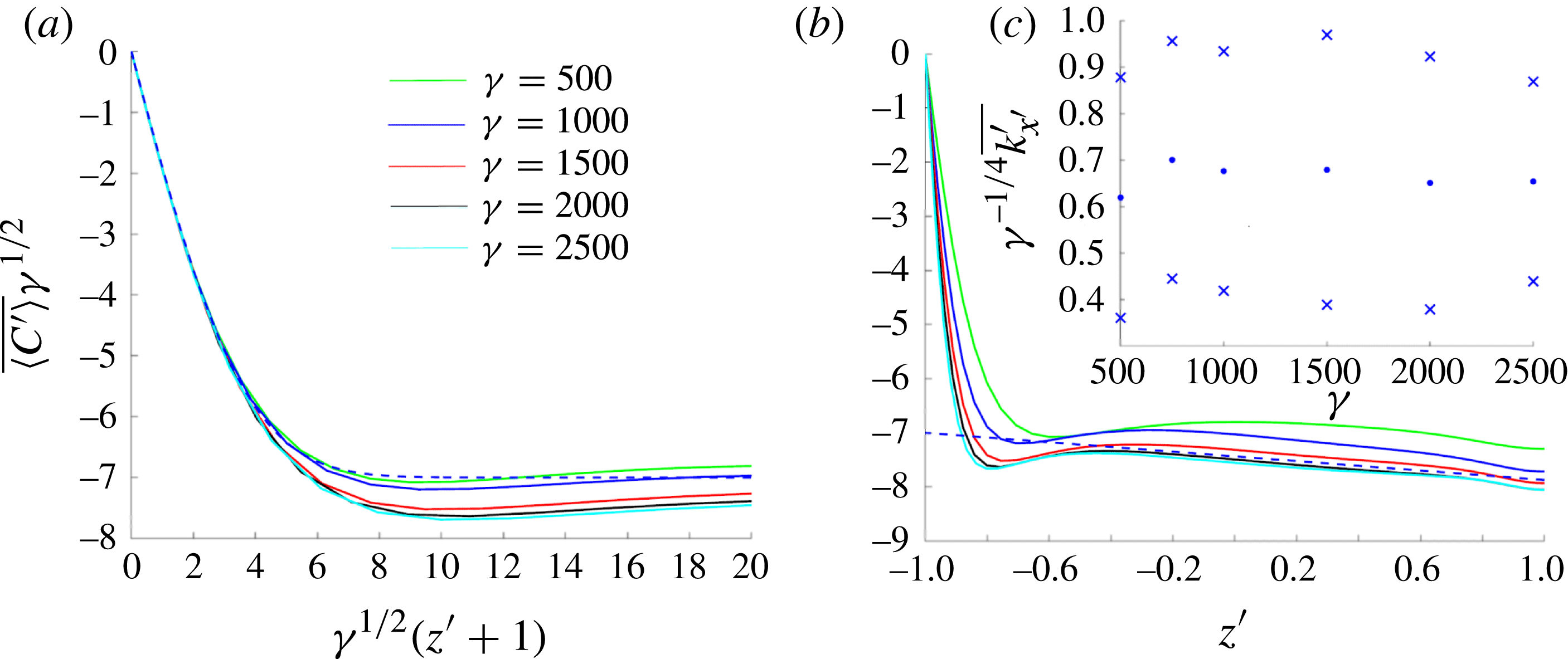
For larger
 ${\it\gamma}$
, the upper boundary layer becomes increasingly active. The averaged concentration profile in the boundary layer again resembles a graph of an error function and has a penetration depth of
 $O({\it\gamma}^{-1/2})$
(figure 10
a). We expect that for
 ${\it\gamma}\gg 1$
the penetration depth of the upper boundary layer will be sufficiently small for the reaction of solute to be negligible; the time- and horizontally averaged concentration profile decays approximately linearly outside the boundary layer (figure 10
b).
Profile of the horizontally and time-averaged concentration field plotted against (a)
 ${\it\gamma}^{1/2}(z^{\prime }+1)$
and (b)
 $z^{\prime }$
for
 $\mathscr{L}=4{\rm\pi}$
. The error-function approximation (5.1) (dashed) is plotted in panel (a) with
 ${\it\alpha}^{\prime }={\it\alpha}_{0}^{\prime }{\it\gamma}$
,
 ${\it\alpha}_{0}^{\prime }=0.125$
and
 ${\it\lambda}^{\prime }=7$
. The dashed line in panel (b) is
 $\overline{C^{\prime }}{\it\gamma}^{1/2}=-{\it\lambda}^{\prime }-\tilde{k}^{\prime 2}(1+z^{\prime })$
with
 $\tilde{k}^{\prime }=0.66$
. The inset panel (c) suggests that the time-averaged wavenumber evaluated at
 $z^{\prime }=0$
scales like
 ${\it\gamma}^{1/4}$
; dots and crosses show mean and standard deviation, respectively.

To characterise the plumes, we again follow Slim (Reference Slim2014) and estimate the mean wavenumber of plumes by defining
 ${\hat{C}}^{\prime }=C^{\prime }-\langle C^{\prime }\rangle$
and computing the time average
 $\overline{k_{x^{\prime }}^{\prime }}$
and variance of
 $\sqrt{\langle {\hat{C}}_{x^{\prime }}^{\prime 2}\rangle /\langle {\hat{C}}^{\prime 2}\rangle }$
. The data in figure 10(c) suggest that the wavenumber is approximately
 $0.66{\it\gamma}^{1/4}$
for
 ${\it\gamma}\gg 1$
, although there are appreciable fluctuations around this mean value.
3.3. Finite domain depth:
$\mathit{Da}=O(1)$
,
$\mathit{Ra}\gg 1$


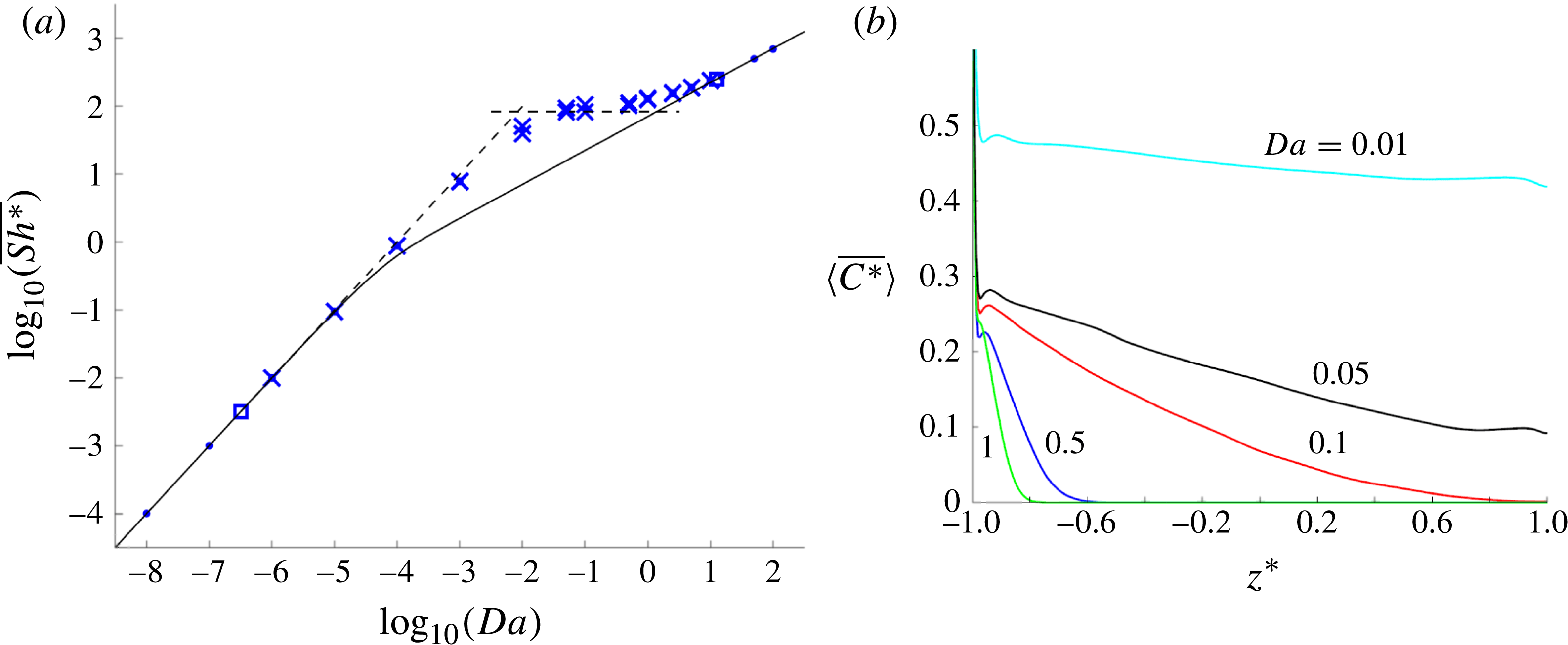
Figure 11(a) shows
 $\overline{\mathit{Sh}^{\ast }}$
calculated from solutions to (2.1) and (2.2) for
 $\mathit{Ra}=5000$
. The uptake rate exceeds the value corresponding to the no-flow state (2.15) when convection is established and
 $\mathit{Da}$
is sufficiently large. For
 $\mathit{Da}<{\it\gamma}_{c}/Ra^{2}\approx 3.1\times 10^{-7}$
and
 $\mathit{Da}>{\it\beta}_{c}^{2}/\mathit{Ra}\approx 12.5$
, the no-flow state is linearly stable and the concentration field is approximated by the horizontally uniform base state (2.15), with
 $\mathit{Sh}^{\ast }=2\mathit{Ra}\,\mathit{Da}$
and
 $\mathit{Sh}^{\ast }=\sqrt{\mathit{Ra }\,\mathit{Da}}$
, respectively. Figure 11(a) illustrates how the no-flow solutions connect smoothly to the asymptotes
 $\mathit{Sh}^{\ast }\approx 2\mathit{Ra}\,\mathit{Da}$
(for
 $\mathit{Ra}^{-2}\ll \mathit{Da}\ll 1$
) and
 $\mathit{Sh}^{\ast }\approx 0.017\mathit{Ra}$
(for
 $1\ll \mathit{Da}\ll \mathit{Ra}$
; see figure 7), and that there is a further smooth connection between these asymptotes for
 $\mathit{Da}=O(1)$
(numerically, this is around
 $\mathit{Da}\approx 0.01$
). To understand this transition, figure 11(b) shows profiles of
 $\overline{\langle C^{\ast }\rangle }(z^{\ast })$
for
 $\mathit{Ra}=5000$
and increasing
 $\mathit{Da}$
. This illustrates three distinct regimes: the deep-domain case for larger
 $\mathit{Da}$
, characterised by the concentration profile decaying to zero at
 $z^{\ast }=z_{0}^{\ast }<1$
(as in figure 4); the shallow-domain case for smaller
 $\mathit{Da}$
, characterised by
 $\overline{\langle C^{\ast }\rangle }$
being approximately uniform across the majority of the domain (as in figure 10
b); and an intermediate regime characterised by
 $\overline{\langle C^{\ast }\rangle }$
decaying to zero close to
 $z^{\ast }=1$
. Previous simulations by Andres & Cardoso (Reference Andres and Cardoso2012) confirm that convective mixing becomes increasingly important as
 $\mathit{Da}$
decreases and the system transitions from a pure conductive state with flux
 $\sqrt{\mathit{Ra }\,\mathit{Da}}$
to the plateau with flux
 $0.017\mathit{Ra}$
.
(a) Time-averaged
 $\overline{\mathit{Sh}^{\ast }}$
(dots)
 $\pm$
one standard deviation (crosses) obtained from solutions to (2.1) and (2.2) for
 $\mathit{Ra}=5000$
. In some instances dots are obscured by crosses. The solid line shows the no-flow
 $\mathit{Sh}^{\ast }$
(2.15); squares mark points of neutral stability of the no-flow state; dashed lines show the shallow-domain approximation
 $\overline{\mathit{Sh}}^{\ast }=2\mathit{Ra}\,\mathit{Da}$
from (2.14) for
 $\mathit{Da}<10^{-2}$
and the deep-domain approximation
 $\overline{\mathit{Sh}}^{\ast }=0.017\mathit{Ra}$
from (4.6) for
 $\mathit{Da}>10^{-2}$
. (b) Time- and horizontally averaged concentrations
 $\langle \overline{C^{\ast }}\rangle (z^{\ast })$
for values of
 $\mathit{Da}$
as shown.

The states presented so far represent a large-time statistical equilibrium between the flux from the source at the upper boundary and solute uptake within the domain. In appendix B, we present the solution to an initial-value problem for
 $\mathit{Ra}=5000$
and
 $\mathit{Da}=10^{-5}$
when little solute is initially in the domain, illustrating how the system passes through successive regimes of plume growth. With such a low
 $\mathit{Da}$
, these solutions recapitulate many features of the non-reactive one-sided convection problem of Slim (Reference Slim2014) before reaching a statistically constant steady state.
We now analyse the large-time flow structures in more detail, starting with the deep-domain case.
4. The structure of the deep-domain flow
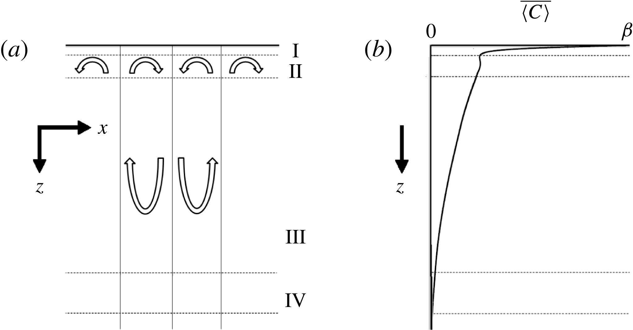
Figure 12 illustrates the likely structure of the flow when
 ${\it\beta}\gg 1$
(cf. figure 4). We anticipate four regions: an active boundary layer at the top of the domain of depth
 $O(1/{\it\beta})$
(region I; see figure 4
a), which is kept thin by upwelling flows from beneath; a region containing long slender plumes of depth
 $O({\it\beta})$
(region III; figure 4), in which advection balances horizontal diffusion and uptake; an intermediate region linking regions I and III, where the tops of the plumes recirculate (region II); and a region near the tip of the large plumes where the concentration falls to zero (region IV). We conjecture that regions II and IV include flow structures with order-unity aspect ratio, and that region II in particular is inherently dynamic. We present approximations of the flow in the elongated regions (I and III), which are sufficient to characterise the primary features of the flow.
Schematic of the flow structure for
 ${\it\beta}\gg 1$
showing (a) the recirculation cells about one of the larger plumes and (b) the time- and horizontally averaged concentration profile. The kink in the concentration profile is observed in simulations but not explained by the simplified model.

4.1. Upwelling boundary-layer flow (region I)
To gain some insight into the mechanism by which disturbances grow in the boundary layer near
 $z=0$
, we make the very crude assumption that, locally,
 ${\it\psi}\approx {\it\alpha}xz$
(representing the upwelling between two plumes, centred on
 $x=0$
without loss of generality), for some strain rate
 ${\it\alpha}({\it\beta})$
. Assuming
 $C\approx C(z)$
, (2.7) becomes
 $$\begin{eqnarray}-{\it\alpha}zC_{z}=C_{zz}-C.\end{eqnarray}$$
When
 ${\it\alpha}$
is large, the boundary-layer depth is thin and the dominant balance in (4.1) becomes
 $-{\it\alpha}zC_{z}=C_{zz}$
. Imposing
 $C={\it\beta}$
on
 $z=0$
and
 $C_{z}\rightarrow 0$
for large
 $z$
, (2.7) (with the uptake term neglected) is satisfied exactly by
 $$\begin{eqnarray}C_{0}(z)={\it\beta}-(1-{\it\lambda}){\it\beta}\,\text{erf}(({\it\alpha}/2)^{1/2}z),\quad {\it\psi}_{0}(x,z)={\it\alpha}xz.\end{eqnarray}$$
Here
 $0<{\it\lambda}<1$
is a constant such that
 $C\rightarrow {\it\lambda}{\it\beta}$
for large
 $z$
. We expect the boundary-layer thickness, of order
 ${\it\alpha}^{-1/2}$
in (4.2), to be
 $O({\it\beta})$
(from figure 4
a), so we set
 ${\it\alpha}={\it\alpha}_{0}{\it\beta}^{2}$
. The simulations in figure 4(a) are then well approximated by (4.2) with
 ${\it\alpha}_{0}\approx 8\times 10^{-4}$
and
 ${\it\lambda}\approx 0.25$
. Since the surface flow in figure 4(c) is dominated by regions of upwelling (where
 ${\it\psi}_{xz}>0$
) in comparison to downwelling, it is reasonable to estimate the solute flux per unit length through the upper boundary as
 $$\begin{eqnarray}\mathit{Sh}=-C_{0z}(0)=(1-{\it\lambda}){\it\beta}^{2}(2{\it\alpha}_{0}/{\rm\pi})^{1/2}.\end{eqnarray}$$
These values of
 ${\it\alpha}_{0}$
and
 ${\it\lambda}$
are consistent with the approximation
 $\overline{\mathit{Sh}}\approx 0.017{\it\beta}^{2}$
demonstrated in figure 7(a).
The time- and horizontally averaged vertical velocity profile scales with
 ${\it\beta}$
over a distance
 $1/{\it\beta}$
, consistent with (4.2b
) (data not shown), which is sufficient to maintain a thin concentration boundary layer. The time-averaged horizontal velocity field scales as order
 ${\it\beta}$
(consistent with snapshots shown in figure 4(c)), a factor
 ${\it\beta}$
smaller than suggested by (4.2b
). However
 ${\it\psi}_{0xz}(x,0)={\it\alpha}_{0}{\it\beta}^{2}$
provides a satisfactory approximation to the instantaneous surface strain rate where the flow is upwelling (figure 4
c). The flux at the outer edge of the boundary layer is dominated by concentrated downwellings of high concentration, which are not included in the present analysis.
To consider how
 ${\it\alpha}_{0}$
and
 ${\it\lambda}$
are related, we follow the spirit of Malkus (Reference Malkus1954) and Howard (Reference Howard and Görtler1964) and seek a condition under which the local boundary-layer solution (4.2) is neutrally stable. To investigate its linear stability, we write
 $$\begin{eqnarray}C=C_{0}(z)+\bar{C}(\bar{x},\bar{z},\bar{t}),\quad {\it\psi}={\it\psi}_{0}(x,z)+{\it\alpha}^{-1/2}\bar{{\it\psi}}(\bar{x},\bar{z},\bar{t}),\end{eqnarray}$$
where
 $(\bar{x},\bar{z})={\it\alpha}^{1/2}(x,z)$
and
 $\bar{t}={\it\alpha}t$
. Here, we allow for disturbances to vary over horizontal distances comparable to the boundary-layer depth (see figure 4
d), to capture the growth of small plumes. Then, neglecting terms that are quadratic in
 $\bar{C}$
and
 $\bar{{\it\psi}}$
, and discarding
 $O(1/{\it\beta}^{2})$
terms associated with uptake, (2.7) becomes
 $$\begin{eqnarray}\displaystyle \bar{C}_{\bar{t}}+\bar{x}\bar{C}_{\bar{x}}-\bar{z}\bar{C}_{\bar{z}}+{\rm\Delta}\text{e}^{-\bar{z}^{2}/2}\bar{{\it\psi}}_{\bar{x}}=\bar{C}_{\bar{x}\bar{x}}+\bar{C}_{\bar{z}\bar{z}},\quad \bar{{\it\psi}}_{\bar{x}\bar{x}}+\bar{{\it\psi}}_{\bar{z}\bar{z}}=-\bar{C}_{\bar{x}}, & & \displaystyle\end{eqnarray}$$
with boundary conditions
 $$\begin{eqnarray}\displaystyle \bar{C}=0\quad \text{on}\ \bar{z}=0, & \quad & \displaystyle \bar{C}\rightarrow 0\quad \text{as}\ \bar{z}\rightarrow \infty ,\end{eqnarray}$$
 $$\begin{eqnarray}\displaystyle \bar{{\it\psi}}=0\quad \text{on}\ \bar{z}=0, & \quad & \displaystyle \bar{{\it\psi}}\rightarrow 0\quad \text{as}\ \bar{z}\rightarrow \infty ,\end{eqnarray}$$
where
 ${\it\Delta}\equiv (1-{\it\lambda})/({\rm\pi}{\it\alpha}_{0}/2)^{1/2}$
. The term proportional to
 ${\it\Delta}$
involves vertical flow perturbations disturbing the base concentration profile, generating horizontal concentration gradients that drive a flow that reinforces the perturbation. This is modified by advection and horizontal stretching of the perturbation by the base straining flow as well as solute diffusion. Consequently
 ${\it\Delta}$
measures the excitability of the boundary layer. We therefore seek the value
 ${\it\Delta}_{c}$
(or a range of values) for which the boundary layer is neutrally stable (or nearly so), which will connect the parameters
 ${\it\alpha}_{0}$
and
 ${\it\lambda}$
. From (4.3), the flux per unit length through the boundary layer at neutral stability can then be written as
 $$\begin{eqnarray}\mathit{Sh}=\frac{2(1-{\it\lambda})^{2}{\it\beta}^{2}}{{\rm\pi}{\it\Delta}_{c}}={\it\alpha}_{0}{\it\Delta}_{c}{\it\beta}^{2}.\end{eqnarray}$$
Our previous estimates of
 ${\it\lambda}$
and
 ${\it\alpha}_{0}$
suggest that
 ${\it\Delta}_{c}\approx 21.2$
.
To interpret this value, we initially solve (4.5a–c
) neglecting the
 $\bar{x}$
advection term in (4.5a
): this problem is then homogeneous in
 $\bar{x}$
and solutions that grow exponentially in time can be computed. These are neutrally stable for
 ${\it\Delta}_{c}\approx 14.6$
with wavenumber
 $\bar{k}_{\bar{x}}\approx 1.54$
, as explained in appendix C. While encouraging, this approximation neglects the limited range in
 $\bar{x}$
and
 $\bar{t}$
over which perturbations may grow, represented by the ribs in the fishbone plot in figure 3.
4.2. Optimal perturbations of the boundary layer
For a more realistic assessment of the stability of (4.5a–c
), we seek solutions of the form
 $\bar{C}=\bar{C}({\it\xi},\bar{z},\bar{t})$
,
 $\bar{{\it\psi}}=\bar{{\it\psi}}({\it\xi},\bar{z},\bar{t})$
, where
 ${\it\xi}=\bar{x}\exp (-\bar{t})$
. This eliminates the
 $\bar{x}$
advection term but introduces time-dependent coefficients to terms with
 ${\it\xi}$
derivatives. We then make a Fourier decomposition in
 ${\it\xi}$
, writing solutions as
 $$\begin{eqnarray}\bar{C}={\hat{C}}(\bar{z},\bar{t})\,\text{e}^{\text{i}\bar{k}_{{\it\xi}}{\it\xi}},\quad \bar{{\it\psi}}=-\text{i}\hat{{\it\psi}}(\bar{z},\bar{t})\,\text{e}^{\text{i}\bar{k}_{{\it\xi}}{\it\xi}},\end{eqnarray}$$
for some wavenumber
 $\bar{k}_{{\it\xi}}$
. Substituting (4.7) into (4.5a
) gives the system
 $$\begin{eqnarray}\displaystyle & {\hat{C}}_{\bar{t}}-\bar{z}{\hat{C}}_{\bar{z}}+{\it\Delta}\bar{k}_{{\it\xi}}\text{e}^{-\bar{z}^{2}/2-\bar{t}}\hat{{\it\psi}}-{\hat{C}}_{\bar{z}\bar{z}}+\bar{k}_{{\it\xi}}^{2}\text{e}^{-2\bar{t}}{\hat{C}}=0, & \displaystyle\end{eqnarray}$$
 $$\begin{eqnarray}\displaystyle & \hat{{\it\psi}}_{\bar{z}\bar{z}}-\bar{k}_{{\it\xi}}^{2}\text{e}^{-2\bar{t}}\hat{{\it\psi}}-\bar{k}_{{\it\xi}}\text{e}^{-\bar{t}}{\hat{C}}=0, & \displaystyle\end{eqnarray}$$
 $$\begin{eqnarray}\displaystyle {\hat{C}}=0\quad \text{on}\ \bar{z}=0, & \quad & \displaystyle {\hat{C}}\rightarrow 0\quad \text{as}\ \bar{z}\rightarrow \infty ,\end{eqnarray}$$
 $$\begin{eqnarray}\displaystyle \hat{{\it\psi}}=0\quad \text{on}\ \bar{z}=0, & \quad & \displaystyle \bar{{\it\psi}}\rightarrow 0\quad \text{as}\ \bar{z}\rightarrow \infty .\end{eqnarray}$$
 $\bar{z}$
and
 $\bar{t}$
parametrised by
 $\bar{k}_{{\it\xi}}$
and
 ${\it\Delta}$
.
To investigate (4.8) and (4.9), we choose a wavenumber and an initial concentration distribution and then seek to maximise the square of the concentration perturbation integrated over the
 $\bar{z}$
domain at some later time
 $\bar{T}$
. Here
 $\bar{T}$
is chosen to represent the time taken for a disturbance to grow at the centre of an upwelling region and to be swept towards a nearby concentration hotspot at the base of a large plume. (Of course, the approximation
 ${\it\psi}={\it\alpha}xz$
will not be uniformly valid across this region, but it provides a useful initial approximation.) We define a Lagrangian that maximises the growth factor
 $\Vert \boldsymbol{q}(\bar{T})\Vert ^{2}/\Vert \boldsymbol{q}_{0}\Vert ^{2}$
, subject to constraints (4.8) and (4.9), as explained in appendix D. This involves solving the forward problem (4.8) and (4.9), the backward problem given by its adjoint, and using a power method to iterate over the initial condition,
 $\boldsymbol{q}_{0}$
, to find the initial state that maximises the growth factor (following Schmid (Reference Schmid2007)).
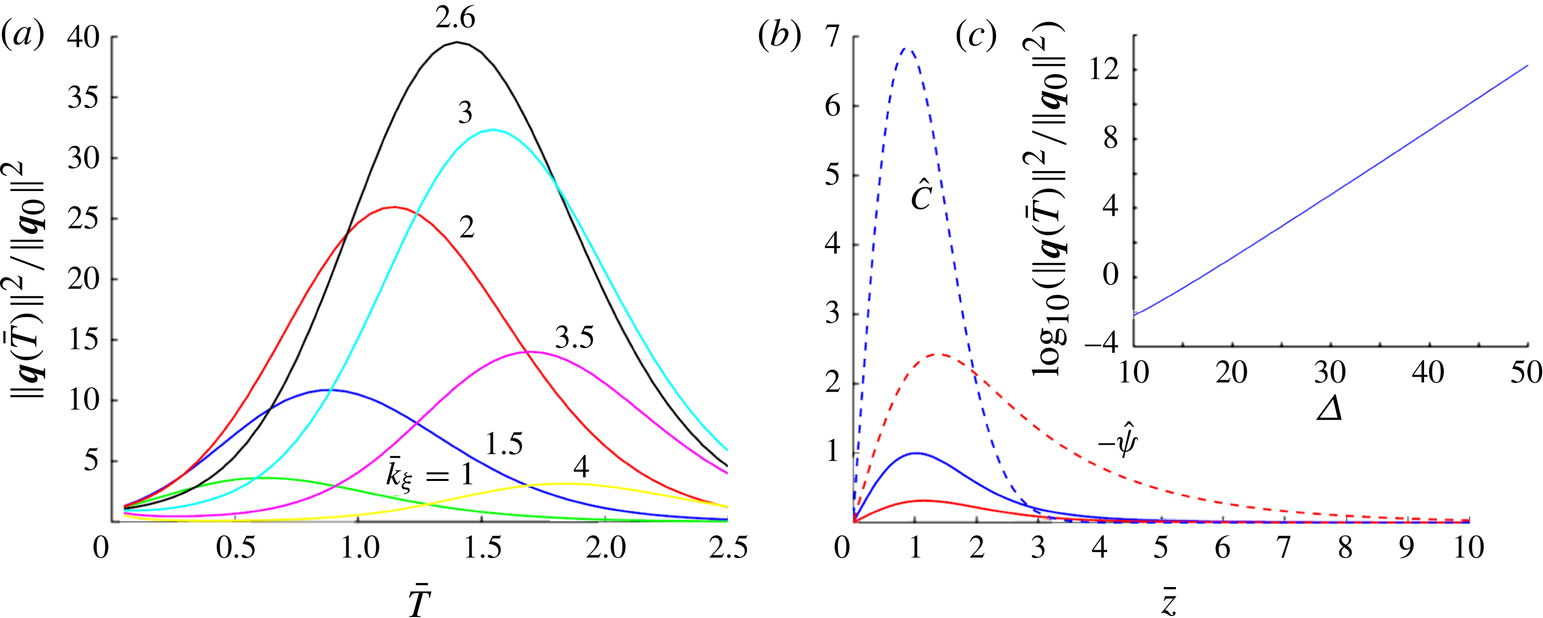
Figure 13(a) presents solutions to (4.8) and (4.9) showing the growth factor of perturbations over a range of
 $\bar{T}$
using
 ${\it\Delta}=21.2$
for different wavenumbers. Over a time interval
 $\bar{T}=1.6$
, for example, corresponding to a
 $t$
interval 0.05 (a typical rib lifetime in figure 3
a), disturbances with
 $\bar{k}_{{\it\xi}}\approx 2.6$
show the greatest growth. Figure 13(b) shows the concentration and streamfunction profiles at
 $\bar{t}=0$
and
 $\bar{t}=\bar{T}$
corresponding to the optimal perturbation for
 $\bar{T}=1.6$
. Figure 13(c) shows how the amplification of such disturbances grows rapidly with
 ${\it\Delta}$
.
(a) Growth factor amplification over different time intervals
 $\bar{T}$
for given wavenumbers for
 ${\it\Delta}=21.2$
. (b) Concentration and streamfunction profiles corresponding to the initial (solid) perturbation and final (dashed) perturbation for
 $\bar{T}=1.6$
,
 $\bar{k}_{{\it\xi}}=2.6$
. The inset panel (c) shows how the growth factor increases dramatically for a moderate increase in
 ${\it\Delta}$
for
 $\bar{k}_{{\it\xi}}=2.6$
,
 $\bar{T}=1.6$
.

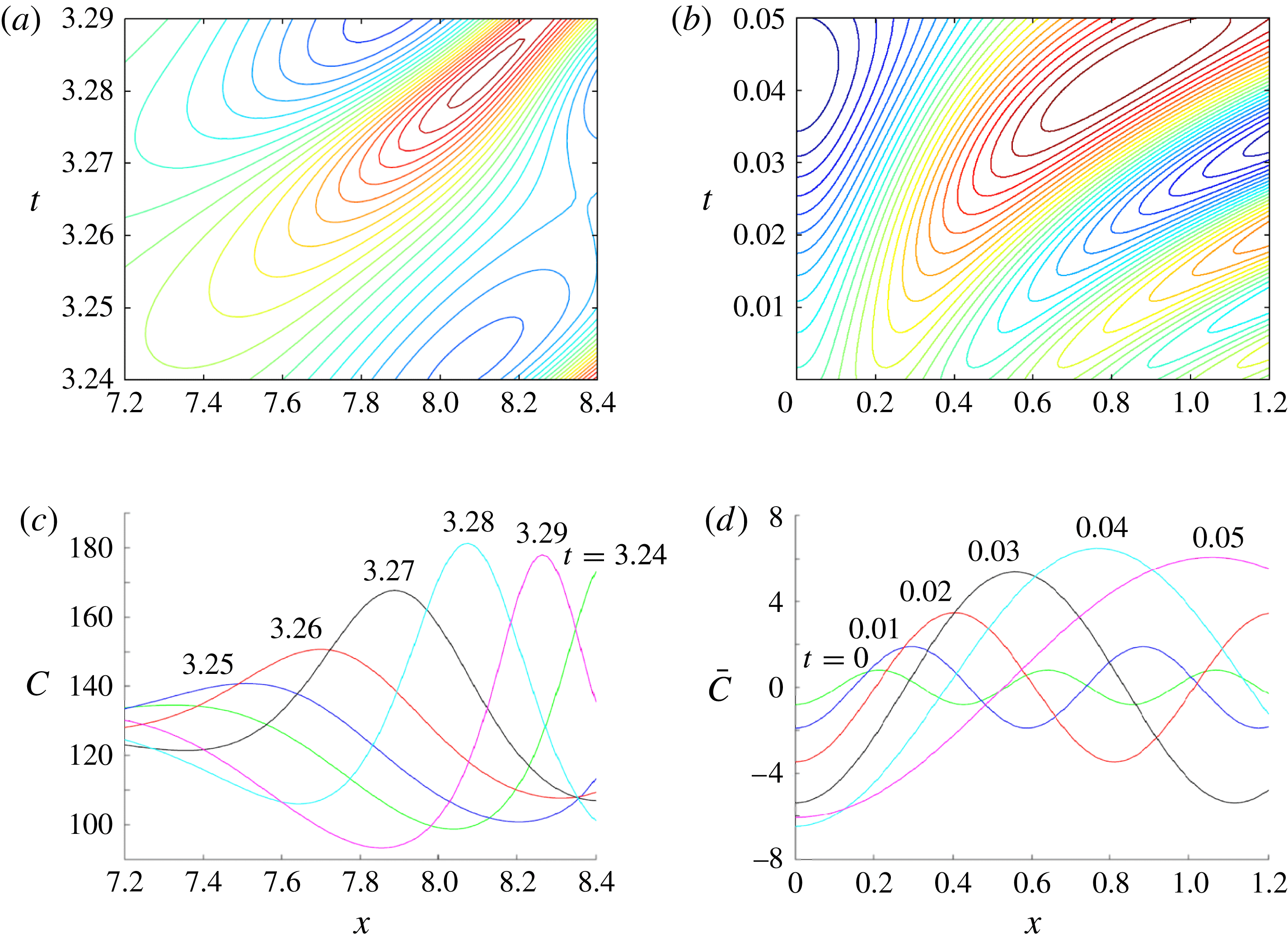
Figure 14(a,c) shows the evolution of a single rib from the fishbone plot in figure 3(a). To illustrate the solution shown in figure 13(b) more clearly, figure 14(b,d) shows the solution to (4.8) and (4.9) with
 $\bar{k}_{{\it\xi}}=2.6$
with
 ${\it\Delta}=21.2$
in the domain
 $\bar{x}\in [0,{\rm\pi}/3]$
. Clearly, the assumption of a simple extensional flow
 ${\it\psi}={\it\alpha}xz$
is not uniformly valid, as the ribs in figure 14(a) appear to travel at a steady speed as they increase in amplitude rather than accelerating in figure 14(b), and the linear optimal growth calculation at fixed wavenumber
 $\bar{k}_{{\it\xi}}$
cannot capture the non-sinusoidal shape evident in figure 14(c). Thus the parameters chosen are at best illustrative of likely behaviour. Nevertheless, the estimate of disturbance wavenumber is not unreasonable, while figure 13(c) shows that disturbances of this wavenumber amplify exponentially with
 ${\it\Delta}$
over a given time interval.
(a) A magnification of the space–time plot of figure 3, showing the evolution of a rib for
 ${\it\beta}=200$
. (c) Concentration magnitudes are shown at times indicated. (b,d) Equivalent maps of the concentration field
 $\bar{C}$
(see (4.7)) reconstructed using optimally amplified solutions to (4.8), for
 ${\it\Delta}=21.2$
,
 $\bar{T}=1.6$
,
 $\bar{k}_{{\it\xi}}=2.6$
, and rescaled using
 ${\it\alpha}={\it\alpha}_{0}{\it\beta}^{2}$
,
 ${\it\alpha}_{0}=8\times 10^{-4}$
,
 ${\it\beta}=200$
. In all cases variables are plotted against
 $(x,t)$
coordinates.

The Malkus–Howard idea of the boundary layer being close to neutral stability is helpful in supporting the chosen scalings. However, simulations (figure 3) suggest that the boundary layer operates in a state slightly above neutral stability, particularly at larger
 ${\it\beta}$
, so that disturbances grow appreciably as they are swept towards the base of the nearest large plume, but not so much that the boundary layer is profoundly disrupted. This suggests that
 ${\it\Delta}$
can be expected to occupy a range of values. This calculation therefore provides evidence that taking
 ${\it\Delta}\approx 21.2$
is consistent with simulation data, but does not provide a definitive prediction of
 ${\it\Delta}_{c}$
in (4.6).
We now connect the boundary-layer solution of § 4.1 to the large plumes below.
4.3. Slender plumes (region III)
The plumes that penetrate deep into the domain have depth
 $O({\it\beta})$
(figure 4
b) and width
 $O(1)$
(figures 5 and 6). To describe them, we seek steady solutions of (2.7) and (2.8) using a Reynolds decomposition of the form
 $C=\langle C\rangle (z)+{\hat{C}}(x,z)$
, where
 $\langle {\hat{C}}\rangle =0$
, in a domain
 $-L/2<x<L/2$
(where
 $L$
is the width of a plume and
 $x=0$
is now chosen to be the centre of a plume). Assuming that horizontal diffusion dominates vertical diffusion (the assumption used in ‘heat-exchanger’ approximations in the Rayleigh–Bénard problem by Hewitt et al. (Reference Hewitt, Neufeld and Lister2012) and Slim (Reference Slim2014)), and imposing the condition
 $[{\it\psi}]_{-L/2}^{L/2}=0$
(implying no mean vertical flow), (2.7) can be integrated to give
 $$\begin{eqnarray}{\it\psi}_{x}=-{\hat{C}},\end{eqnarray}$$
with
 $$\begin{eqnarray}{\it\psi}_{z}{\hat{C}}_{x}+{\hat{C}}(\langle C\rangle _{z}+{\hat{C}}_{z})={\hat{C}}_{xx}-\langle C\rangle -{\hat{C}}.\end{eqnarray}$$
Taking the horizontal average of (4.11) gives
 $$\begin{eqnarray}\langle {\it\psi}_{z}{\hat{C}}_{x}\rangle +\langle {\hat{C}}{\hat{C}}_{z}\rangle =-\langle C\rangle ,\end{eqnarray}$$
which with (4.11) gives
 $$\begin{eqnarray}({\it\psi}_{z}{\hat{C}}_{x}-\langle {\it\psi}_{z}{\hat{C}}_{x}\rangle )+{\hat{C}}\langle C\rangle _{z}+({\hat{C}}{\hat{C}}_{z}-\langle {\hat{C}}{\hat{C}}_{z}\rangle )={\hat{C}}_{xx}-\hat{C.}\end{eqnarray}$$
Correspondingly, the dominant contribution to the mean vertical flux is
 $J(z)=-\langle {\it\psi}_{x}{\hat{C}}\rangle$
. Assuming uptake is negligible in regions I and II relative to that in region III, we may set
 $\overline{\mathit{Sh}}=J(0)$
.
Assuming
 ${\it\psi}=-f(z)\sin (kx)$
and
 ${\hat{C}}=g(z)\cos (kx)$
, where
 $g\geqslant 0$
and
 $k=2{\rm\pi}/L$
, equations (4.10), (4.12) and (4.13) reduce exactly to
 $$\begin{eqnarray}k\,f=g,\quad gg_{z}=-\langle C\rangle ,\quad g[\langle C\rangle _{z}+(1+k^{2})]=0,\end{eqnarray}$$
with
 $J={\textstyle \frac{1}{2}}g^{2}$
. Equation (4.14b
) shows how convective fluxes balance the reactive decay of the mean concentration field, while (4.14c
) shows that the flow partitions into domains in which
 $g=0$
(in
 $z>z_{0}$
, say) and
 $g>0$
(in
 $0\leqslant z<z_{0}$
). We assume that
 $\langle C\rangle \rightarrow 0$
and
 $g\rightarrow 0$
as
 $z\rightarrow z_{0}-$
, so that
 $\langle C\rangle =(1+k^{2})(z_{0}-z)$
in
 $0\leqslant z<z_{0}$
, and hence
 $g=(1+k^{2})^{1/2}(z_{0}-z)$
in this region. Thus
 $$\begin{eqnarray}C=(z_{0}-z)[(1+k^{2})+(1+k^{2})^{1/2}\cos (kx)],\quad {\it\psi}=-(z_{0}-z)\frac{(1+k^{2})^{1/2}}{k}\sin (kx)\end{eqnarray}$$
in
 $0<z<z_{0}$
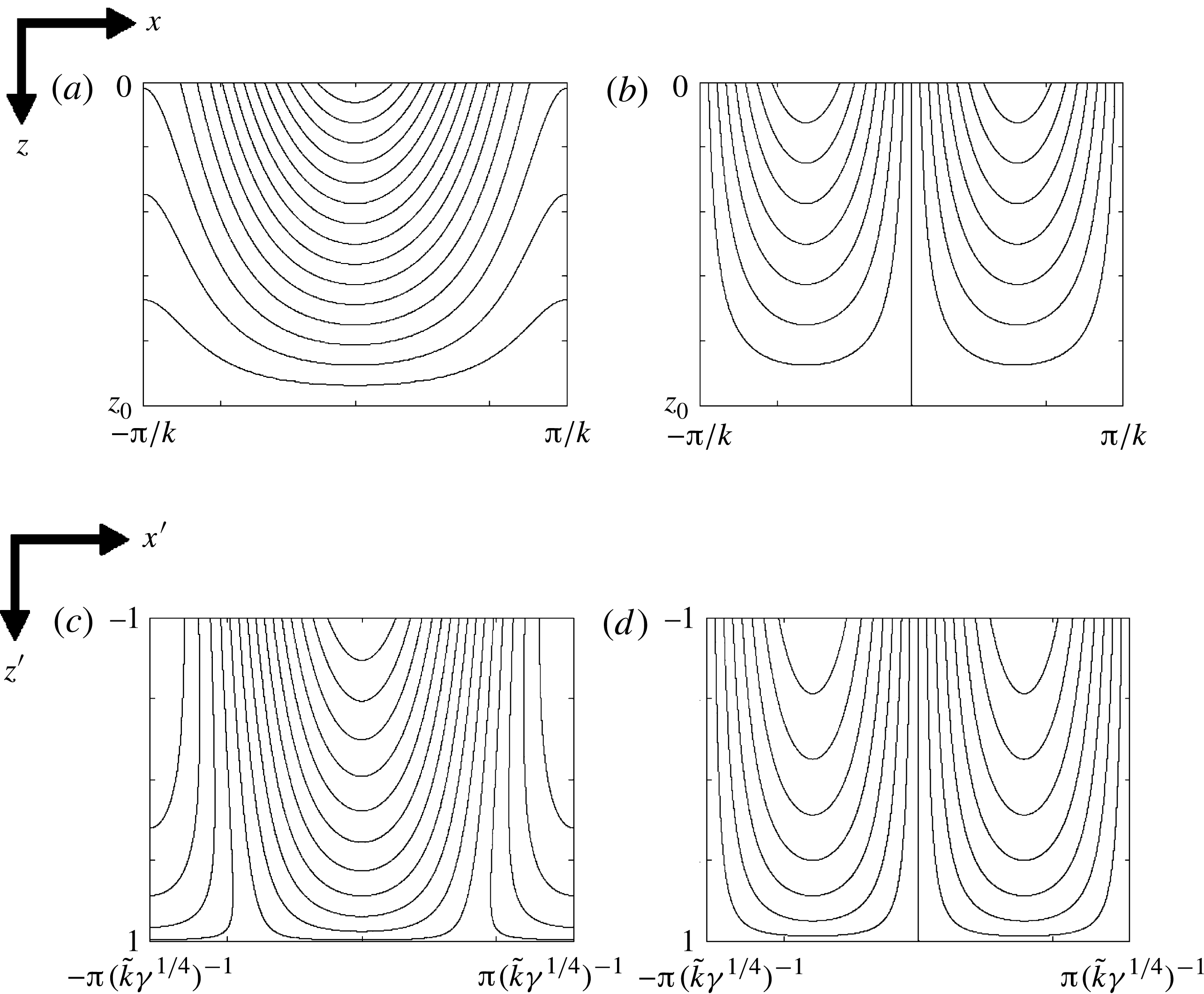
. This turns out to be a locally exact nonlinear solution to (2.7); unlike some others who have developed similar approximations, we are not required to make a closure assumption. Figure 15(a,b) shows an example of a solution to (4.15) for
 $L=4{\rm\pi}$
. Solutions capture the sinusoidal behaviour illustrated in figure 6(a,b), but do not incorporate the recirculation at the tops of plumes evident in figure 2.
(a,b) Plumes for the deep-domain case, showing (a) concentration perturbation and (b) streamfunction, using (4.15), with
 $z_{0}={\it\zeta}{\it\beta}$
,
 ${\it\zeta}=0.125$
,
 ${\it\beta}=200$
and
 $k=1.08$
. (c,d) Plumes for the shallow-domain case, using (5.8), with
 $\tilde{k}=0.66$
,
 $\tilde{C}_{0}=-{\it\lambda}^{\prime }-\tilde{k}^{2}$
,
 ${\it\lambda}^{\prime }=7$
and
 ${\it\gamma}=1000$
.

The horizontally averaged vertical flux satisfies
 $J={\textstyle \frac{1}{2}}(z_{0}-z)^{2}(1+k^{2})$
, so at the top of region III one has
 $J(0)=z_{0}^{2}(1+k^{2})/2$
. Matching the flux per unit length through the boundary layer (4.6) to that in the plume is consistent with simulation data of figures 4(b) and 5, which suggests that
 $k=O(1)$
and
 $z_{0}\approx {\it\zeta}{\it\beta}$
, where
 ${\it\zeta}\approx 0.125$
; with existing estimates for
 ${\it\lambda}$
and
 ${\it\Delta}_{c}$
, matching predicts
 $k\approx 1.08$
, which is consistent with numerical estimates in figure 5 at the top of region III. In addition, one can match the leading-order average concentration in (4.15) to the outer limit of the boundary layer, giving
 $z_{0}(1+k^{2})\approx {\it\lambda}{\it\beta}$
, i.e.
 ${\it\zeta}(1+k^{2})={\it\lambda}$
, which again fits with numerical estimates of the parameters. However, it is unclear at present how the streamfunction in (4.15) might connect to the straining flow in the boundary layer; this requires assessment of the recirculating flow in region II. At present we simply observe that the
 $O({\it\beta})$
vertical flow at the top of region III balances the
 $O({\it\beta})$
vertical and horizontal time-averaged flow outside the boundary layer, whereas the
 $O({\it\beta}^{2})$
(or larger) strain rates in the boundary layer (figure 4
c) arise through dynamic effects.
Overall, therefore, this analysis provides a self-consistent (albeit incomplete) description of regions I and III, with four relations that link the five parameters
 ${\it\lambda}$
,
 ${\it\alpha}_{0}$
,
 ${\it\Delta}$
,
 ${\it\zeta}$
and
 $k$
:
 $$\begin{eqnarray}{\it\Delta}={\it\Delta}_{c},\quad 1+k^{2}=\frac{{\it\lambda}^{2}{\rm\pi}{\it\Delta}}{4(1-{\it\lambda})^{2}},\quad {\it\alpha}_{0}=\frac{2(1-{\it\lambda})^{2}}{{\rm\pi}{\it\Delta}^{2}},\quad {\it\zeta}=\frac{{\it\lambda}}{1+k^{2}}.\end{eqnarray}$$
The predicted flux is
 $\overline{\mathit{Sh}_{0}}\approx {\textstyle \frac{1}{2}}(1+k^{2}){\it\zeta}^{2}={\it\alpha}_{0}{\it\Delta}_{c}$
. We anticipate that vertical diffusion will be significant in a passive boundary layer at the base of the plume, smoothing the transition from a linear average concentration profile to zero (region IV in figure 12). Regions I–III of the assumed flow structure resemble features proposed in a scaling argument by Neufeld et al. (Reference Neufeld, Hesse, Riaz, Hallworth, Tchelepi and Huppert2010) for non-reactive convection, except that the down- and upwellings have equal width in the present problem and the intrinsically dynamic nature of region II precludes a quasi-steady mass balance, requiring instead consideration of the stability of the boundary layer in region I. Further analysis, for example of plume stability (Hewitt et al.
Reference Hewitt, Neufeld and Lister2013b
) and of the intermediate region II, is needed to make this approximation fully predictive, but is not pursued further here.
5. The structure of the shallow-domain flow
We anticipate that solutions to the shallow-domain problem (2.11) and (2.12) have a similar structure to figure 12, except that plumes penetrate to the lower boundary of the domain, placing the region-IV boundary layer along
 $z^{\prime }=1$
.
5.1. Boundary-layer flow (region I)
As with the deep-domain case, we assume that the upper boundary layer is fully developed and governed by (2.11) with
 $C^{\prime }=0$
and
 ${\it\psi}^{\prime }=0$
on
 $z^{\prime }=-1$
. Assuming near
 $z^{\prime }=-1$
in upwelling regions that
 ${\it\psi}^{\prime }\approx {\it\alpha}^{\prime }x^{\prime }(z^{\prime }+1)/{\it\gamma}$
for some constant
 ${\it\alpha}^{\prime }$
and
 $C^{\prime }=C^{\prime }(z^{\prime })$
, and following similar reasoning to that in § 4.1, (2.11) with the reaction term neglected is satisfied by
 $$\begin{eqnarray}C_{0}^{\prime }(z^{\prime })=-{\it\lambda}^{\prime }{\it\gamma}^{-1/2}\,\text{erf}(({\it\alpha}^{\prime }/2)^{1/2}(z^{\prime }+1)),\quad {\it\psi}_{0}^{\prime }={\it\alpha}^{\prime }x^{\prime }(z^{\prime }+1)/{\it\gamma},\end{eqnarray}$$
for some
 ${\it\lambda}^{\prime }$
such that
 $C^{\prime }\rightarrow -{\it\lambda}^{\prime }{\it\gamma}^{-1/2}$
for large
 $z^{\prime }$
. The constraint (2.14) on the flux, which we assume applies to the base-state boundary layer, requires that
 $$\begin{eqnarray}\overline{\mathit{Sh}^{\prime }}=-C_{0z}^{\prime }(-1)={\it\lambda}^{\prime }(2{\it\alpha}^{\prime }/{\rm\pi}{\it\gamma})^{1/2}=2.\end{eqnarray}$$
Both (5.2) and figure 10(a) suggest that the boundary-layer depth is
 $O({\it\gamma}^{-1/2})$
. Setting
 ${\it\alpha}^{\prime }\approx {\it\alpha}_{0}^{\prime }{\it\gamma}$
, and matching (5.1) to the simulation data in figure 10(a) gives
 ${\it\alpha}_{0}^{\prime }\approx 0.125$
and
 ${\it\lambda}^{\prime }\approx 7$
, which are reasonably consistent with the constraint
 ${\it\lambda}^{\prime 2}{\it\alpha}_{0}^{\prime }=2{\rm\pi}$
from (5.2).
Assuming solutions of the form
 $$\begin{eqnarray}C^{\prime }=C_{0}^{\prime }(z^{\prime })+\bar{C}^{\prime }(\bar{x}^{\prime },\bar{z}^{\prime },\bar{t}^{\prime }),\quad {\it\psi}^{\prime }={\it\psi}_{0}^{\prime }(x^{\prime },z^{\prime })+({\it\alpha}^{\prime })^{-1/2}\bar{{\it\psi}}^{\prime }(\bar{x}^{\prime },\bar{z}^{\prime },\bar{t}^{\prime }),\end{eqnarray}$$
where
 $(\bar{x}^{\prime },\bar{z}^{\prime })={\it\alpha}^{\prime 1/2}(x^{\prime },z^{\prime }+1)$
and
 $\bar{t}^{\prime }={\it\alpha}^{\prime }t^{\prime }$
, linearising (2.11) about the steady state and discarding
 $O(1/{\it\alpha}^{\prime })$
terms associated with uptake yields (4.5a–c
) with
 ${\it\Delta}$
replaced by
 ${\it\Delta}^{\prime }={\it\lambda}^{\prime }(2/({\rm\pi}{\it\alpha}_{0}^{\prime }))^{1/2}={\it\lambda}^{\prime 2}/{\rm\pi}$
. The existing numerical estimate of
 ${\it\lambda}^{\prime }$
gives
 ${\it\Delta}^{\prime }\approx 16$
, which is again close to values at which the boundary layer can be expected to be weakly unstable according to figure 13.
5.2. Slender plumes (region III)
For
 ${\it\gamma}\gg 1$
, noting the wavenumber scaling in figure 10(c), we set
 $C^{\prime }=\tilde{C}^{\prime }/{\it\gamma}^{1/2}$
,
 ${\it\psi}^{\prime }=\tilde{{\it\psi}}^{\prime }/{\it\gamma}^{3/4}$
,
 $x^{\prime }=\tilde{x}^{\prime }/{\it\gamma}^{1/4}$
,
 $z^{\prime }=\tilde{z}^{\prime }$
and seek a steady slender-plume solution to (2.11) and (2.12). With error
 $O({\it\gamma}^{-1/2})$
, (2.11) becomes
 $$\begin{eqnarray}\tilde{{\it\psi}}_{\tilde{z}^{\prime }}^{\prime }\tilde{C}_{\tilde{x}^{\prime }}^{\prime }-\tilde{{\it\psi}}_{\tilde{x}^{\prime }}^{\prime }\tilde{C}_{\tilde{z}^{\prime }}^{\prime }=\tilde{C}_{\tilde{x}^{\prime }\tilde{x}^{\prime }}^{\prime }-1,\quad \tilde{{\it\psi}}_{\tilde{x}^{\prime }\tilde{x}^{\prime }}^{\prime }=-\tilde{C}_{\tilde{x}^{\prime }}^{\prime }.\end{eqnarray}$$
The vertical flux satisfies
 $J^{\prime }=-{\it\gamma}{\it\psi}_{x^{\prime }}^{\prime }C^{\prime }-{C^{\prime }}_{z^{\prime }}=-\tilde{{\it\psi}}_{\tilde{x}^{\prime }}^{\prime }\tilde{C}^{\prime }+O({\it\gamma}^{-1/2})$
. Again assuming solutions of the form
 $\tilde{C}^{\prime }(\tilde{x}^{\prime },\tilde{z}^{\prime })=\langle \tilde{C}^{\prime }\rangle (\tilde{z}^{\prime })+{\hat{C}}^{\prime }(\tilde{x}^{\prime },\tilde{z}^{\prime })$
, where
 $\langle {\hat{C}}^{\prime }\rangle =0$
and
 $\langle \tilde{{\it\psi}}_{x^{\prime }}^{\prime }\rangle =0$
, (5.4b
) becomes
 $$\begin{eqnarray}\tilde{{\it\psi}}_{\tilde{z}^{\prime }}^{\prime }{\hat{C}}_{\tilde{x}^{\prime }}^{\prime }+{\hat{C}}^{\prime }(\langle \tilde{C}^{\prime }\rangle _{\tilde{z}^{\prime }}+{\hat{C}}_{\tilde{z}^{\prime }}^{\prime })={\hat{C}}_{\tilde{x}^{\prime }\tilde{x}^{\prime }}^{\prime }-1,\quad \tilde{{\it\psi}}_{\tilde{x}^{\prime }}^{\prime }=-{\hat{C}}^{\prime }.\end{eqnarray}$$
Averaging (5.5) and subtracting the average from (5.5) gives
 $$\begin{eqnarray}\displaystyle & \langle \tilde{{\it\psi}}_{\tilde{z}^{\prime }}^{\prime }{\hat{C}}_{\tilde{x}^{\prime }}^{\prime }\rangle +\langle {\hat{C}}^{\prime }{\hat{C}}_{\tilde{z}^{\prime }}^{\prime }\rangle =-1, & \displaystyle\end{eqnarray}$$
 $$\begin{eqnarray}\displaystyle & (\tilde{{\it\psi}}_{\tilde{z}^{\prime }}^{\prime }{\hat{C}}_{\tilde{x}^{\prime }}^{\prime }-\langle \tilde{{\it\psi}}^{\prime }{\hat{C}}_{\tilde{x}^{\prime }}^{\prime }\rangle )+{\hat{C}}^{\prime }\langle \tilde{C}^{\prime }\rangle _{\tilde{z}^{\prime }}+({\hat{C}}^{\prime }{\hat{C}}_{\tilde{z}^{\prime }}^{\prime }-\langle {\hat{C}}^{\prime }{\hat{C}}_{\tilde{z}^{\prime }}^{\prime }\rangle )={\hat{C}}_{\tilde{x}^{\prime }\tilde{x}^{\prime }}^{\prime }. & \displaystyle\end{eqnarray}$$
 $\tilde{{\it\psi}}^{\prime }=-f^{\prime }(\tilde{z}^{\prime })\sin (\tilde{k}^{\prime }\tilde{x}^{\prime })$
and
 ${\hat{C}}^{\prime }=g^{\prime }(\tilde{z}^{\prime })\cos (\tilde{k}^{\prime }\tilde{x}^{\prime })$
yields
 $$\begin{eqnarray}g^{\prime }=f^{\prime }\tilde{k}^{\prime },\quad g^{\prime }g_{\tilde{z}^{\prime }}^{\prime }=-1,\quad g^{\prime }[\langle \tilde{C}^{\prime }\rangle _{\tilde{z}^{\prime }}+\tilde{k}^{\prime 2}]=0.\end{eqnarray}$$
The vertical flux satisfies
 $J_{\tilde{z}^{\prime }}^{\prime }={\textstyle \frac{1}{2}}g^{\prime 2}$
, so we impose
 $g^{\prime }=0$
on
 $\tilde{z}^{\prime }=1$
, implying that
 $g^{\prime 2}=2(1-\tilde{z}^{\prime })$
. This automatically satisfies the constraint
 $J^{\prime }=2$
on
 $\tilde{z}^{\prime }=-1$
, consistent with (2.14). In addition,
 $\langle \tilde{C}^{\prime }\rangle =\tilde{C}_{0}^{\prime }-\tilde{k}^{\prime 2}\tilde{z}^{\prime }$
. In the original variables, this gives the following approximation for the plumes:
 $$\begin{eqnarray}\displaystyle & \displaystyle C^{\prime }={\it\gamma}^{-1/2}[\tilde{C}_{0}^{\prime }-\tilde{k}^{\prime 2}z^{\prime }+\sqrt{2}(1-z^{\prime })^{1/2}\cos (\tilde{k}^{\prime }{\it\gamma}^{1/4}x^{\prime })], & \displaystyle\end{eqnarray}$$
 $$\begin{eqnarray}\displaystyle & \displaystyle {\it\psi}^{\prime }=-(\sqrt{2}/{\it\gamma}^{3/4}\tilde{k}^{\prime })(1-z^{\prime })^{1/2}\sin (\tilde{k}^{\prime }{\it\gamma}^{1/4}x^{\prime }). & \displaystyle\end{eqnarray}$$
 $\tilde{C}_{0}^{\prime }+\tilde{k}^{\prime 2}=-{\it\lambda}^{\prime }$
, again giving four conditions for five parameters. The estimate
 $\tilde{k}^{\prime }\approx 0.66$
from time-averaged simulations (figure 10
c) supports the proposed scaling of wavenumber with
 ${\it\gamma}^{1/4}$
. The plume structure (5.8) for these parameters is illustrated in figure 15(c,d).
6. Flow structure for
$\mathit{Da}=O(1)$
,
$\mathit{Ra}\gg 1$


In order to demonstrate how the shallow- and deep-domain cases are related, we briefly investigate the structure of the flow in the intermediate case with
 $\mathit{Da}=O(1)$
and
 $\mathit{Ra}\gg 1$
, considering solutions of the full system (2.1) and (2.2).
As seen previously, uptake is not significant in region I, and so the boundary layer is expected to have the structure seen in §§ 4.1 and 5.1. Setting
 ${\it\psi}^{\ast }={\it\alpha}^{\ast }x^{\ast }(z^{\ast }+1)$
,
 $C^{\ast }=C^{\ast }(z^{\ast })$
and imposing
 $C^{\ast }\rightarrow {\it\lambda}^{\ast }(\mathit{Da})$
at the outer edge of the boundary layer yields an error-function distribution for
 $C^{\ast }$
over a length scale
 $({\it\alpha}^{\ast }Ra)^{-1/2}$
. Perturbations to this base state then satisfy (4.5a–c
) with
 ${\it\Delta}$
replaced by
 ${\it\Delta}^{\ast }\equiv (1-{\it\lambda}^{\ast })(2/{\rm\pi}{\it\alpha}_{0}^{\ast })^{1/2}$
, where
 ${\it\alpha}^{\ast }={\it\alpha}_{0}^{\ast }(\mathit{Da})\mathit{Ra}$
, giving uptake rate
 $$\begin{eqnarray}\overline{\mathit{Sh}^{\ast }}=(1-{\it\lambda}^{\ast })Ra(2{\it\alpha}_{0}^{\ast }/{\rm\pi})^{1/2}={\it\Delta}^{\ast }{\it\alpha}_{0}^{\ast }\mathit{Ra}.\end{eqnarray}$$
This expression illustrates neatly how the solute transfer is related to the strain rate of the upwelling flow,
 ${\it\alpha}_{0}^{\ast }(\mathit{Da})$
, and the excitability of the boundary layer,
 ${\it\Delta}^{\ast }(\mathit{Da})$
. We anticipate that
 ${\it\Delta}^{\ast }$
lies in the range in which the boundary layer is close to neutral stability. We do not seek to determine the functions
 ${\it\lambda}^{\ast }(\mathit{Da})$
,
 ${\it\alpha}_{0}^{\ast }(\mathit{Da})$
and
 ${\it\Delta}^{\ast }(\mathit{Da})$
in detail here, except to note their limiting forms. For large
 $\mathit{Da}$
,
 ${\it\lambda}_{0}^{\ast }\rightarrow {\it\lambda}$
,
 ${\it\Delta}^{\ast }\rightarrow {\it\Delta}$
and
 ${\it\alpha}_{0}^{\ast }\rightarrow {\it\alpha}_{0}$
, matching with the deep-domain solution and ensuring that
 $\overline{\mathit{Sh}^{\ast }}\rightarrow 0.017\mathit{Ra}$
. For small
 $\mathit{Da}$
,
 ${\it\lambda}^{\ast }\rightarrow 1-\mathit{Da}^{1/2}{\it\lambda}^{\prime }$
,
 ${\it\Delta}^{\ast }\rightarrow {\it\Delta}^{\prime }$
and
 ${\it\alpha}^{\ast }\rightarrow Da{\it\alpha}_{0}^{\prime }$
, ensuring that
 $\overline{\mathit{Sh}^{\ast }}\rightarrow 2\mathit{Ra}\,\mathit{Da}$
.
To address the plume structure, we set
 $x^{\ast }=x^{\star }/\mathit{Ra}^{1/2}$
(choosing
 $x^{\star }=0$
to align with the centre of a plume),
 $z^{\ast }=z^{\star }$
,
 ${\it\psi}^{\ast }={\it\psi}^{\star }/\mathit{Ra}^{1/2}$
and
 $C^{\ast }=C^{\star }$
. Then to
 $O(\mathit{Ra}^{-1})$
, equations (2.1) and (2.2) (at steady state) become
 $$\begin{eqnarray}{\it\psi}_{z^{\star }}^{\star }C_{x^{\star }}^{\star }-{\it\psi}_{x^{\star }}^{\star }C_{z^{\star }}^{\star }=C_{x^{\star }x^{\star }}^{\star }-\mathit{Da}C^{\star },\quad {\it\psi}_{x^{\star }x^{\star }}^{\star }=-C_{x^{\star }}^{\star },\end{eqnarray}$$
with vertical flux
 $J^{\star }/Ra=-{\it\psi}_{x^{\star }}^{\star }C^{\star }+O(\mathit{Ra}^{-1})$
. Once again, vertical diffusion is subdominant to horizontal diffusion. The averaging procedure employed in §§ 5.2 and 4.3 may again be employed. Assuming solutions are of the form
 $$\begin{eqnarray}C^{\star }=\langle C^{\star }\rangle (z^{\star })+g^{\star }(z^{\star })\cos (k^{\star }x^{\star }),\quad {\it\psi}^{\star }=-f^{\star }(z^{\star })\sin (k^{\star }x^{\star })\end{eqnarray}$$
for some wavenumber
 $k^{\star }(\mathit{Da})$
, we can derive the analogues of (4.14) and (5.7), namely
 $$\begin{eqnarray}g^{\star }=k^{\star }f^{\star },\quad g^{\star }g_{z^{\star }}^{\star }=-\mathit{Da}\,\langle C^{\star }\rangle ,\quad g^{\star }[\langle C^{\star }\rangle _{z^{\star }}+(k^{\star 2}+\mathit{Da})]=0,\end{eqnarray}$$
while the average vertical flux is
 $J^{\star }/Ra={\textstyle \frac{1}{2}}g^{\star 2}$
; we can estimate
 $\overline{\mathit{Sh}^{\ast }}$
using
 $J^{\star }$
evaluated at
 $z^{\star }=-1$
. Thus either
 $g^{\star }=0$
or
 $$\begin{eqnarray}\langle C^{\star }\rangle =(k^{\star 2}+\mathit{Da})(z_{0}^{\star }-z^{\star }),\quad g^{\star 2}=Da(k^{\star 2}+\mathit{Da})((z^{\star }-z_{0}^{\star })^{2}-(z_{1}^{\star }-z_{0}^{\star })^{2}),\end{eqnarray}$$
for some constants
 $z_{0}^{\star }(\mathit{Da})$
and
 $z_{1}^{\star }(\mathit{Da})$
; matching the mean concentration with the outer limit of the boundary layer requires
 $(k^{\star 2}+\mathit{Da})(z_{0}^{\star }+1)={\it\lambda}^{\ast }<1$
. Thus the time- and horizontally averaged concentration profiles in figure 11(b) can be approximated by linear functions
 $\langle C^{\star }\rangle =(z_{0}^{\star }-z^{\star }){\it\lambda}^{\ast }/(z_{0}^{\star }+1)$
, so that decreasing
 $\mathit{Da}$
decreases the slope by increasing
 $z_{0}^{\star }$
, initially from values below 1 for which the plumes terminate within the domain, to above 1 for which plumes extend to the base of the domain.
To connect this to the deep-domain solution for large
 $\mathit{Da}$
, we impose
 $\langle C^{\star }\rangle =0$
and
 $g^{\star }=0$
at
 $z^{\star }=z_{1}^{\star }=z_{0}^{\star }\leqslant 1$
. Then (6.5) implies that
 $$\begin{eqnarray}g^{\star }=(\mathit{Da}(k^{\star 2}+\mathit{Da}))^{1/2}(z_{0}^{\star }-z^{\star }),\quad \overline{\mathit{Sh}^{\ast }}\approx {\textstyle \frac{1}{2}}\mathit{Ra\,Da}(k^{\star 2}+\mathit{Da})(z_{0}^{\star }+1)^{2}.\end{eqnarray}$$
The solution corresponds to (4.15) with
 $k^{\star }=\mathit{Da}^{1/2}k$
and
 $z_{0}^{\star }=-1+{\it\zeta}/\mathit{Da}$
for large
 $\mathit{Da}$
, implying that the plume penetration distance from the upper boundary is
 ${\it\zeta}/\mathit{Da}$
. A necessary condition for this solution to be valid is
 $\mathit{Da}>{\it\zeta}/2\approx 0.06$
. The associated flux is
 $\overline{\mathit{Sh}^{\ast }}={\textstyle \frac{1}{2}}\mathit{Ra}(1+k^{2}){\it\zeta}^{2}$
.
Alternatively, plumes penetrate to the bottom boundary at
 $z^{\star }=1$
when
 $\mathit{Da}$
is sufficiently small, in which case we impose
 $g^{\star }=0$
at
 $z^{\star }=z_{1}^{\star }=1$
and take
 $z_{0}^{\star }\geqslant 1$
. In this case (6.5) becomes
 $$\begin{eqnarray}g^{\star 2}=Da(k^{\star 2}+\mathit{Da})(z^{\star }-1)(z^{\star }+1-2z_{0}^{\star }),\quad \overline{\mathit{Sh}^{\ast }}\approx 2\mathit{Ra\,Da}(k^{\star 2}+\mathit{Da})z_{0}^{\star }.\end{eqnarray}$$
To recover the shallow-domain solution for
 $\mathit{Da}\ll 1$
, we set
 $k^{\star }=\tilde{k}^{\prime }\mathit{Da}^{1/4}$
and
 $z_{0}^{\star }=(1+\mathit{Da}^{1/2}\tilde{C}_{0}^{\prime })/\mathit{Da}^{1/2}\tilde{k}^{\prime 2}$
, in which case the leading-order concentration field recovers (5.8). This yields the leading-order flux
 $\overline{\mathit{Sh}^{\ast }}\approx 2\mathit{Ra}\,\mathit{Da}$
.
7. Discussion
Table 1 summarises the main results of this study. We have investigated three distinct regimes of fully established convection at high
 $\mathit{Ra}$
: the deep-domain case (
 $1\ll \mathit{Da}\ll \mathit{Ra}$
), the shallow-domain case
 $\mathit{Ra}^{-2}\ll \mathit{Da}\ll 1$
and the intermediate case (with
 $\mathit{Da}$
of order unity). Our simulations have necessarily been restricted to a finite range of parameters and we cannot rule out that different structures and scalings may emerge at even higher values of
 $\mathit{Ra}$
. However, over the range of parameters investigated, our simulations and analysis suggest that the time-averaged uptake rate
 $\overline{\mathit{Sh}^{\ast }}$
follows the classical scaling, namely being proportional to
 $\mathit{Ra}$
when convection has reached statistically steady state. However,
 $\overline{\mathit{Sh}^{\ast }}$
has a strong dependence on
 $\mathit{Da}$
, as shown in figure 11. In the deep-domain case, simulations suggest that the flux is identical (at leading order) to that arising in classical one-sided Rayleigh–Bénard–Darcy convection during intervals when the lower boundary has no influence (Slim Reference Slim2014). This provides evidence that the flux in this regime is restricted by the boundary layer (or at least by the regions I and II), and that the plumes beneath accommodate this constraint. In the shallow-domain case, however, the limited capacity of the domain to absorb solute restricts the uptake rate and
 $\overline{\mathit{Sh}^{\ast }}$
falls dramatically to
 $2\mathit{Ra}\,\mathit{Da}$
. In this limit, the flow is so weak that convective mixing has negligible impact on the leading-order uptake rate. The estimate
 $\overline{\mathit{Sh}^{\ast }}={\it\Delta}^{\ast }{\it\alpha}_{0}^{\ast }\mathit{Ra}$
in (6.1), where the order-unity parameter
 ${\it\Delta}^{\ast }$
measures the excitability of the boundary layer, supports the notion that the flux weakens as the strain rate
 ${\it\alpha}^{\ast }$
of the upwelling flow in the boundary layer diminishes.
Summary of leading-order scalings of the mean uptake rate
 $\overline{\mathit{Sh}^{\ast }}$
, the wavenumber of large plumes
 $k^{\ast }$
, the plume penetration depth
 $1+z_{0}^{\ast }$
, the average subsurface concentration
 $\overline{C_{-}^{\ast }}$
just outside the boundary layer and the strain rate
 ${\it\alpha}^{\ast }$
of the flow in the boundary layer; numerical estimates of the constants
 $k$
,
 $\tilde{k}$
,
 ${\it\zeta}$
,
 ${\it\lambda}$
,
 ${\it\lambda}^{\prime }$
,
 ${\it\alpha}_{0}$
and
 ${\it\alpha}_{0}^{\prime }$
are given in the text.
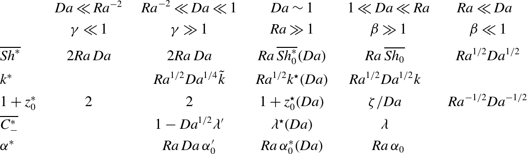
Simulations and theory suggest that the wavenumber of large plumes in all three cases follows the scaling
 $\mathit{Ra}^{1/2}$
(table 1), which differs slightly from the
 $\mathit{Ra}^{0.4}$
scaling reported for the Rayleigh–Bénard–Darcy problem (Hewitt et al.
Reference Hewitt, Neufeld and Lister2013b
). Although there is additional dependence on
 $\mathit{Da}$
, such that the plume wavelength increases as
 $\mathit{Da}$
falls, the plumes always remain slender structures. Figure 5 illustrates the difficulty of identifying the wavenumber precisely: the measure (3.1), for a time-evolving nonlinear flow, is necessarily amplitude-dependent, even though the time-averaged plumes have a clear sinusoidal structure (figure 6). The penetration depth
 $1+z_{0}^{\ast }$
of plumes falls as
 $\mathit{Da}$
increases, but is independent of
 $\mathit{Ra}$
. In the deep-domain case, mixing increases the plume length substantially relative to the penetration depth of the no-flow base state.
The boundary layer at the upper domain boundary is characterised by a rapid drop in concentration over a vertical distance of order
 $1/\mathit{Ra}$
when
 $\mathit{Da}\gtrsim 1$
(the boundary-layer thickness increases to order
 $1/(\mathit{Ra}\,\mathit{Da}^{1/2})$
for
 $\mathit{Ra}^{-2}\ll \mathit{Da}\ll 1$
). In the deep-domain case the subsurface concentration drops to approximately 25 % of its surface value; in the shallow-domain case, the drop is much smaller (
 $O(\mathit{Da}^{1/2})$
), indicating increasing saturation of the medium with solute. The strain rate of the flow near the upper wall, arising from upwelling between plumes, always scales like
 $\mathit{Ra}$
(table 1) but falls in strength as the layer becomes shallow. At any instant, the horizontal velocity field within the boundary layer is heterogeneous (figure 4
c) and dynamic. However, an approximate stability analysis (§ 4.2) suggests that the wavelength of disturbances that grow into small plumes within the boundary layer scales with the boundary-layer depth, i.e. like
 $1/\mathit{Ra}$
in the deep-domain case (confirmed by measurements of plume wavenumber in the boundary layer in figure 4
d) and
 $1/(\mathit{Ra}\,\mathit{Da}^{1/2})$
in the shallow-domain case.
Plot of
 $\mathit{Sh}^{\ast }$
computed from a time-dependent solution with solute initially added to the top of the domain for
 $\mathit{Ra}=5000$
,
 $\mathit{Da}=10^{-5}$
and
 $\mathscr{L}={\rm\pi}$
. In panel (a) the solid curve (blue online) shows
 $\mathit{Sh}^{\ast }(t^{\ast })$
, and the dashed line (red online) shows
 $\mathit{Ra}\,\mathit{Da}\,M^{\ast }/\mathscr{L}$
. Inset panels (b) and (c) focus on the evolution of
 $\mathit{Sh}^{\ast }$
over early and long time scales, with the horizontal lines illustrating the approximations
 $\mathit{Sh}^{\ast }=0.017\mathit{Ra}$
and
 $\mathit{Sh}^{\ast }=2\mathit{Ra}\,\mathit{Da}$
, respectively. Inset panel (d) shows the horizontally averaged concentration profiles at
 $t^{\ast }=0.5,10,30,250$
and 12 000, respectively.

The approximate theoretical model we have developed explains many features of the observed flow structures but falls short of providing independent estimates of all quantities. The boundary-layer analysis suggests that the flow operates close to marginal stability, but indicates that there is some variability in its excitability between different cases. The coefficient
 ${\it\Delta}$
is estimated to be larger in the deep-domain case than in the shallow-domain case, suggesting that the boundary layer is more active in the former case. In § 4.2 we used a transient-growth analysis to interpret the estimated values of
 ${\it\Delta}$
. This was sufficient to approximate the growth of small-amplitude disturbances but failed to capture features arising at larger amplitudes. The intricate anatomy of multiple interacting ribs and backbones (figure 3
a) awaits further study. The simple heat-exchanger model for the large vertical plumes captures major features of the time-averaged flow and concentration fields. However, the dynamic recirculation in region II has so far defied simple approximation; this region is likely to be key in developing a fully predictive model.
The present study provides a valuable foundation on which to develop further studies relevant to
 $\text{CO}_{2}$
sequestration. For example, the simulation showing the sequence of states through which the system passes before reaching a statistically constant steady state for small
 $\mathit{Da}$
(figure 16) emphasises the importance of understanding transient phenomena. Similarly, it may be important to consider slow changes to the matrix arising from the chemical reaction that degrades the solute. Over long times, the convective patterns investigated here can be expected to degrade the matrix, effectively lowering
 $\mathit{Da}$
in regions that have been exposed to solute for long periods. Provided the domain is sufficiently deep and
 $\mathit{Ra}$
sufficiently high, and assuming there are not dramatic changes to the matrix permeability and porosity, the present model suggests that the solute transfer rate may saturate close to its deep-domain value
 $0.017\mathit{Ra}$
, corresponding to conditions along the plateau in figure 11 for
 $1\ll \mathit{Da}\ll \mathit{Ra}$
. Plumes will penetrate further into the medium as the effective Damköhler number falls, without changing the solute transfer rate, until encountering the base of the domain. Eventually, once the substrate is depleted sufficiently, diminishing the capacity of the domain to absorb additional solute, we expect the solute transfer rate to fall, as the finite domain depth feeds back on the boundary layer (corresponding to shallow-domain behaviour seen in figure 11 for
 $\mathit{Ra}^{-2}\ll \mathit{Da}\ll 1$
). We will report our investigations of this problem in a future study.
Acknowledgements
We acknowledge the invaluable contributions made by Professor A. Cliffe to the early stages of this study, prior to his untimely death in January 2014. We are also grateful to Dr C. A. Rochelle and Dr D. Noy of the British Geological Survey for valuable disussions. This project was in part funded by the Nottingham Centre for Carbon Capture and Storage and the EU FP7 PANACEA project.
Supplementary movie
Supplementary movie is available at http://dx.doi.org/10.1017/jfm.2014.594.
Appendix A. Method: leapfrog time-stepping scheme
Equations (2.1)–(2.2) and (2.11)–(2.12) were solved numerically using a spectral method (Trefethen Reference Trefethen2000), approximating
 $C$
and
 ${\it\psi}$
by
 $N$
Chebyshev polynomials (satisfying the vertical boundary conditions) in the
 $z$
direction and evaluating the governing equations at the Chebyshev collocation points
 $k_{j}=\cos ((2j-1){\rm\pi}/(2N))$
for
 $j=1,\dots ,N$
. To avoid the artificiality of truncating the computational domain in the semi-infinite case (2.7)–(2.8), we simply map the collocation points
 $k_{j}$
to
 ${\it\zeta}_{j}$
, where
 ${\it\zeta}_{j}={\it\sigma}(1+k_{j})/\sqrt{4-(1+k_{j})^{2}}$
for a scaling parameter
 ${\it\sigma}$
that is used to distribute the collocation points such that there is a large number near the top boundary (which we anticipate to be a very active region) with larger spacings deeper into the domain (Boyd Reference Boyd2001). The governing equations were then solved using a leapfrog time-stepping scheme; the deep-domain case is described to illustrate the method.
Fourier series with
 $M$
modes were used to approximate the solutions in the horizontal direction, enforcing periodic boundary conditions along the vertical walls. Solutions to (2.7) and (2.8) are assumed to be of the form
 $$\begin{eqnarray}C(x,z)=\mathop{\sum }\limits_{m=-M/2}^{M/2}C_{m}(z)\exp (2\text{i}m{\rm\pi}x/{\it\Lambda}),\quad {\it\psi}(x,z)=\mathop{\sum }\limits_{m=-M/2}^{M/2}{\it\psi}_{m}(z)\exp (2\text{i}m{\rm\pi}x/{\it\Lambda}).\end{eqnarray}$$
Solving (2.7) and (2.8) in Fourier space decouples the system into
 $M$
linear equations each of order
 $N$
.
Equations (2.7) and (2.8) were evolved in time using a leapfrog scheme requiring two previous solutions (at steps
 $n-1$
and
 $n$
) to find a solution at time step
 $n+1$
. The problem was formulated as follows. The concentration and streamfunction at time step
 $n$
(
 $C^{n},{\it\psi}^{n}$
) were transformed into Fourier space and the first-order derivatives with respect to
 $z$
and
 $x$
were found. These derivatives were transformed into real space, combined to form the nonlinear term in (2.7a
) and transformed back into Fourier space to give the advection term
 $\mathit{Conv}^{n}$
. The
 $m$
th component of (2.7a
) was then solved using
 $$\begin{eqnarray}\frac{C_{m}^{n+1}-C_{m}^{n-1}}{\mathit{d t}/2}+2\,\mathit{Conv}_{m}^{n}=(\text{D}_{zz}-(2m{\rm\pi}/{\it\Lambda})^{2}I)(C_{m}^{n+1}+C_{m}^{n-1})-(C_{m}^{n+1}+C_{m}^{n-1}),\end{eqnarray}$$
where
 $\text{d}t$
is the time step and
 $\text{D}_{zz}$
is the second-order differential operator acting on the rescaled Chebyshev polynomials. Having solved (A 2) for
 $m=-M/2,\dots ,M/2$
, the
 $m$
th component of the corresponding streamfunction was obtained from
 $$\begin{eqnarray}(\text{D}_{zz}-(2m{\rm\pi}/{\it\Lambda})^{2}I){\it\psi}_{m}^{n+1}=-(2\text{i}m{\rm\pi}/{\it\Lambda})C_{m}^{n+1}.\end{eqnarray}$$
We also applied the Robert–Asselin filter to this leapfrog scheme to suppress any computational modes resulting in time-splitting instability (Asselin Reference Asselin1972). The numbers of Chebyshev and Fourier modes were increased and the time-stepping interval was decreased until there was no change in the time- and horizontally averaged solutions. Equation (2.5) also provided useful computational validation of solutions.
Appendix B. The initial-value problem for
$\mathit{Ra}=5000$
,
$\mathit{Da}=10^{-5}$
and
$\mathscr{L}={\rm\pi}$


Figure 16(a) shows the evolution of
 $\mathit{Sh}^{\ast }$
obtained by solving (2.7) and (2.8) for
 $\mathit{Ra}=5000$
,
 $\mathit{Da}=10^{-5}$
and
 $\mathscr{L}={\rm\pi}$
and with little solute initially in the domain. Inset panels (b) and (c) show
 $\mathit{Sh}^{\ast }$
over early and long time scales, respectively, and inset panel (d) shows the horizontally averaged concentration profile at given times.
Initially, a horizontally uniform layer forms across the upper boundary, which diffuses into the domain (see figure 16
d,
 $t^{\ast }=0.5$
). Once the boundary layer has reached a sufficient thickness, it loses stability and small fingers form, which grow vertically downwards.
When the fingers have grown to a sufficient length (corresponding to a local maximum in
 $\mathit{Sh}^{\ast }$
, figure 16
a), neighbouring fingers interact; adjacent fingers merge and the growth of shorter fingers is stunted by the shielding of larger plumes. This results in fewer, thicker plumes. As the plumes descend into the domain, they displace dilute solvent, which is forced upwards between the plumes. Instabilities form in the boundary, which are swept horizontally by the recirculation of the dilute solvent into the base of the larger plumes, feeding the growth of the larger plumes. This regime is characterised by the flux of solute into the domain fluctuating at a value close to
 $\mathit{Sh}^{\ast }=0.017\mathit{Ra}$
(line in figure 16
b), the approximation of
 $\mathit{Sh}^{\ast }$
when
 $\mathit{Ra}\,\mathit{Da}\gg 1$
and similar to the ‘reinitiation regime’ reported by Slim (Reference Slim2014) in simulations of the one-sided Rayleigh–Bénard–Darcy problem. During this regime
 $\langle C^{\ast }\rangle$
takes the form of the horizontally averaged concentration profile when
 $\mathit{Ra}\,\mathit{Da}\gg 1$
(figure 16
d,
 $t^{\ast }=10$
).
As the plumes reach the bottom of the domain, the solute spreads across the lower boundary and connects the plumes (figure 16
d,
 $t^{\ast }=30$
). Once the build-up of solute at the lower boundary is sufficient such that solute-rich fluid is recirculated to the upper boundary, the flux begins to decay. The domain begins to saturate with dissolved solute and the boundary layer at the top of the domain thickens similar to the ‘shutdown regime’ reported in Slim (Reference Slim2014) (figure 16
d,
 $t^{\ast }=250$
).
Over longer time scales the system reaches a statistically steady state at
 $t^{\ast }=T_{0}$
,
 $T_{0}\approx 12\,000$
, at which point
 $\mathit{Sh}^{\ast }$
is approximately equal to
 $\mathit{Ra}\,\mathit{Da}\,M^{\ast }/\mathscr{L}$
(solid and dashed curves in figure 16
c, respectively). In this statistically steady state the flux of solute into the domain approaches
 $\mathit{Sh}^{\ast }=2\mathit{Ra}\,\mathit{Da}$
(horizontal line in figure 16
b), the approximation of
 $\mathit{Sh}^{\ast }$
when
 $\mathit{Da}\ll 1$
,
 $\mathit{Ra}\gg 1$
.
For different Da the evolution of the plumes progresses in a similar manner. For smaller
 $\mathit{Da}$
, when vertical diffusion dominates reaction, it is expected that the box-filling regime corresponding to a decay in
 $\mathit{Sh}^{\ast }$
may continue for a longer time before attaining a statistically steady state. For larger Da the vertical growth of the plumes will eventually be restricted by the reaction of solute and the system will remain in the constant flux regime. However, the time needed to attain a statistically steady state is sensitive to the initial value used.
Appendix C. Solution to (4.5a–c
) with
$\bar{x}$
advection neglected

We consider the simplified case of (4.5a–c
) where the horizontal advection term,
 $\bar{x}\bar{C}_{\bar{x}}$
, is neglected. Assuming solutions of the form
 $$\begin{eqnarray}\bar{C}=\tilde{C}(\bar{z})\exp (\text{i}\bar{k}_{\bar{x}}\bar{x}+{\it\sigma}\bar{t}),\quad \bar{{\it\psi}}=\tilde{{\it\psi}}(\bar{z})\exp (\text{i}\bar{k}_{\bar{x}}\bar{x}+{\it\sigma}\bar{t}),\end{eqnarray}$$
where
 ${\it\sigma}$
and
 $\bar{k}_{\bar{x}}$
are the growth rate and wavenumber, respectively, gives an eigenvalue problem for
 ${\it\sigma}={\it\sigma}(\bar{k}_{\bar{x}},{\it\Delta})$
. The problem was solved using a spectral method, approximating
 $C$
and
 ${\it\psi}$
in
 $z$
as a sum of
 $N$
Chebyshev polynomials and the governing equations evaluated at the Chebyshev collocation points
 $k_{j}=\cos ((2j-1){\rm\pi}/(2N))$
, for
 $j=1,\dots ,N$
, yielding an eigenvalue problem of the form
 ${\it\sigma}\unicode[STIX]{x1D63D}(C,{\it\psi})^{\text{T}}=\unicode[STIX]{x1D63C}(C,{\it\psi})^{\text{T}}$
for some
 $2N\times 2N$
matrices
 $\unicode[STIX]{x1D63C}$
and
 $\unicode[STIX]{x1D63D}$
, following Ward et al. (Reference Ward, Cliffe, Jensen and Power2014).
Figure 17(a) shows the neutral stability curve, indicating the onset of linear instability for
 ${\it\Delta}\approx 14.6$
,
 $\bar{k}_{\bar{x}}\approx 1.54$
; figure 17(b) illustrates the concentration and streamfunction profiles corresponding to these critical values.
(a) The neutral stability curve obtained by solving (4.5a–c
) with no
 $x$
advection, showing the critical value of
 ${\it\Delta}$
for the onset of linear instability. (b) The concentration and streamfunction profiles corresponding to the critical value of
 ${\it\Delta}\approx 14.6$
(corresponding to
 $\bar{k}_{\bar{x}}\approx 1.54$
).

Appendix D. Transient-growth problem
A common method of investigating the stability of unsteady flows is to use an iterative method to find the optimal initial condition resulting in the maximum amplification of perturbation energy over a period of time (Schmid Reference Schmid2007).
To investigate (4.8) and (4.9), we represent the concentration and streamfunction as a vector
 $\boldsymbol{q}=({\hat{C}},\hat{{\it\psi}})^{\text{T}}$
and then define the integral of the scalar product of two such vectors by
 $$\begin{eqnarray}\{\boldsymbol{p},\boldsymbol{q}\}\equiv \int _{0}^{\infty }\boldsymbol{p}^{\text{T}}\boldsymbol{q}\text{d}\bar{z}.\end{eqnarray}$$
Since the streamfunction is slaved to the concentration field by a Poisson equation, we measure disturbance growth using the concentration field alone, via
 $$\begin{eqnarray}\Vert \boldsymbol{q}\Vert ^{2}\equiv \{\boldsymbol{q},\unicode[STIX]{x1D63D}\boldsymbol{q}\},\quad \unicode[STIX]{x1D63D}=\left(\begin{array}{@{}cc@{}}1 & 0\\ 0 & 0\end{array}\right).\end{eqnarray}$$
The governing equations (4.8) are written as
 $\unicode[STIX]{x1D63D}\boldsymbol{q}_{\bar{t}}=\boldsymbol{\mathfrak{L}}\boldsymbol{q}$
where
 $$\begin{eqnarray}\boldsymbol{\mathfrak{L}}=\left(\begin{array}{@{}cc@{}}\partial _{\bar{z}\bar{z}}-k_{{\it\xi}}^{2}\exp (-2\bar{t})+\bar{z}\partial _{\bar{z}} & -{\rm\Delta}k_{{\it\xi}}\exp (-\bar{z}^{2}/2-\bar{t})\\ -k_{{\it\xi}}\exp (-\bar{t}) & \partial _{\bar{z}\bar{z}}-k_{{\it\xi}}^{2}\exp (-2\bar{t})\end{array}\right).\end{eqnarray}$$
The corresponding adjoint operator and adjoint vector are written as
 $$\begin{eqnarray}\boldsymbol{\mathfrak{L}}^{\dagger }=\left(\begin{array}{@{}cc@{}}\partial _{\bar{z}\bar{z}}-k_{{\it\xi}}^{2}\exp (-2\bar{t})-\partial _{\bar{z}}(\bar{z}\cdot ) & -k_{{\it\xi}}\exp (-\bar{t})\\ -{\rm\Delta}k_{{\it\xi}}\exp (-\bar{z}^{2}/2-\bar{t}) & \partial _{\bar{z}\bar{z}}-k_{{\it\xi}}^{2}\exp (-2\bar{t})\end{array}\right),\quad \boldsymbol{q}^{\dagger }=\left(\begin{array}{@{}c@{}}{\hat{C}}^{\dagger }\\ \hat{{\it\psi}}^{\dagger }\end{array}\right).\end{eqnarray}$$
With boundary conditions (4.9), and imposing
 $$\begin{eqnarray}\displaystyle {\hat{C}}^{\dagger }=0\quad \text{on}\ \bar{z}=0, & \quad & \displaystyle {\hat{C}}^{\dagger }\rightarrow 0\quad \text{as}\ \bar{z}\rightarrow \infty ,\end{eqnarray}$$
 $$\begin{eqnarray}\displaystyle \hat{{\it\psi}}^{\dagger }=0\quad \text{on}\ \bar{z}=0, & \quad & \displaystyle \hat{{\it\psi}}^{\dagger }\rightarrow 0\quad \text{as}\ \bar{z}\rightarrow \infty ,\end{eqnarray}$$
 $\{\boldsymbol{q}^{\dagger },\boldsymbol{\mathfrak{L}}\boldsymbol{q}\}=\{\mathfrak{L}^{\dagger }\boldsymbol{q}^{\dagger },\boldsymbol{q}\}$
.
Over an interval
 $0\leqslant \bar{t}\leqslant \bar{T}$
, we wish to maximise the relative disturbance growth by adjusting the initial condition. To achieve this we define the Lagrangian
 $$\begin{eqnarray}\mathbb{L}=\frac{\Vert \boldsymbol{q}(\bar{T})\Vert ^{2}}{\Vert \boldsymbol{q}_{0}\Vert ^{2}}-\int _{0}^{\bar{T}}\{\boldsymbol{q}^{\dagger },(\unicode[STIX]{x1D63D}\partial _{\bar{t}}-\boldsymbol{\mathfrak{L}})\boldsymbol{q}\}\,\text{d}\bar{t}-\{\boldsymbol{q}_{0}^{\dagger },\unicode[STIX]{x1D63D}(\boldsymbol{q}(0)-\boldsymbol{q}_{0})\}.\end{eqnarray}$$
The first term represents the growth factor that we wish to maximise. The second and third terms enforce the governing equations and the initial condition, respectively. The adjoint solution,
 $\boldsymbol{q}^{\dagger }$
, and its initial condition
 $\boldsymbol{q}_{0}^{\dagger }$
act as Lagrange multipliers. Integration by parts yields
 $$\begin{eqnarray}\mathbb{L}=\frac{\Vert \boldsymbol{q}(\bar{T})\Vert ^{2}}{\Vert \boldsymbol{q}_{0}\Vert ^{2}}-\int _{0}^{\bar{T}}\{\boldsymbol{q},(-\unicode[STIX]{x1D63D}\partial _{\bar{t}}-\boldsymbol{\mathfrak{L}}^{\dagger })\boldsymbol{q}^{\dagger }\}\text{d}\bar{t}-\{\boldsymbol{q},\unicode[STIX]{x1D63D}\boldsymbol{q}^{\dagger }\}|_{\bar{T}}+\{\boldsymbol{q},\unicode[STIX]{x1D63D}(\boldsymbol{q}^{\dagger }-\boldsymbol{q}_{0}^{\dagger })\}|_{0}+\{\boldsymbol{q}_{0},\unicode[STIX]{x1D63D}\boldsymbol{q}_{0}^{\dagger }\}.\end{eqnarray}$$
Setting to zero the first variation of
 $\mathbb{L}$
with respect to the independent variables gives equations that define the iterative process used to obtain the optimal initial condition. Enforcing
 ${\it\delta}\mathbb{L}/{\it\delta}\boldsymbol{q}^{\dagger }=0$
and
 ${\it\delta}\mathbb{L}/{\it\delta}\boldsymbol{q}_{0}^{\dagger }=0$
in (D 6) gives
 $$\begin{eqnarray}(\unicode[STIX]{x1D63D}\partial _{\bar{t}}-\boldsymbol{\mathfrak{L}})\boldsymbol{q}=0\quad \text{in}\ 0<\bar{t}<\bar{T},\quad \unicode[STIX]{x1D63D}(\boldsymbol{q}(0)-\boldsymbol{q}_{0})=0,\end{eqnarray}$$
which defines the forward problem; enforcing
 ${\it\delta}\mathbb{L}/{\it\delta}\boldsymbol{q}=0$
and
 ${\it\delta}\mathbb{L}/{\it\delta}\boldsymbol{q}(0)=0$
in (D 7) defines the backward problem
 $$\begin{eqnarray}(\unicode[STIX]{x1D63D}\partial _{\bar{t}}+\boldsymbol{\mathfrak{L}}^{\dagger })\boldsymbol{q}^{\dagger }=0\quad \text{in}\ \bar{T}>\bar{t}>0,\quad \unicode[STIX]{x1D63D}(\boldsymbol{q}^{\dagger }(0)-\boldsymbol{q}_{0}^{\dagger })=0.\end{eqnarray}$$
Noting that
 $$\begin{eqnarray}\frac{\Vert \boldsymbol{q}(\bar{T})\Vert ^{2}}{\Vert \boldsymbol{q}_{0}+{\it\delta}\boldsymbol{q}_{0}\Vert ^{2}}\approx \frac{\Vert \boldsymbol{q}(\bar{T})\Vert ^{2}}{\Vert \boldsymbol{q}_{0}\Vert ^{2}}-\frac{2\Vert \boldsymbol{q}(\bar{T})\Vert ^{2}\{\boldsymbol{q}_{0},\unicode[STIX]{x1D63D}\boldsymbol{q}_{0}\}}{\Vert \boldsymbol{q}_{0}\Vert ^{4}}+\cdots \,,\end{eqnarray}$$
then
 ${\it\delta}\mathbb{L}/{\it\delta}\boldsymbol{q}(\bar{T})=0$
and
 ${\it\delta}\mathbb{L}/{\it\delta}\boldsymbol{q}_{0}=0$
using (D 7) give, respectively,
 $$\begin{eqnarray}\unicode[STIX]{x1D63D}\left(\boldsymbol{q}^{\dagger }(\bar{T})-\frac{2}{\Vert \boldsymbol{q}_{0}\Vert ^{2}}\boldsymbol{q}(\bar{T})\right)=0,\quad \unicode[STIX]{x1D63D}\left(\boldsymbol{q}_{0}^{\dagger }-\frac{2\Vert \boldsymbol{q}(\bar{T})\Vert ^{2}}{\Vert \boldsymbol{q}_{0}\Vert ^{4}}\boldsymbol{q}_{0}\right)=0.\end{eqnarray}$$
The iterative cycle is formulated as follows. Using an initial condition
 $\boldsymbol{q}_{0}$
, equations (D 8) and (4.9) are solved forwards in time for
 $0<\bar{t}<\bar{T}$
using a Crank–Nicolson method to obtain
 $\boldsymbol{q}(\bar{T})$
. Then (D 11a
) provides an initial condition for the backwards problem (D 9) and (D 5), which is solved to obtain
 $\boldsymbol{q}^{\dagger }(0)$
. Equation (D 11b
) is solved using Newton’s method to find a new initial condition for the forward problem, starting the next cycle of the iterative process. The procedure is repeated until convergence is achieved. The final result is the optimal initial condition that maximises the growth factor over a given time interval
 $0<\bar{t}<\bar{T}$
.