1 Introduction
Exploring the dynamics of a thin, flexible plate-like structure subjected to axial flow has been of constant interest to researchers as it can enhance our understanding of natural processes, such as the reconfiguration of plants in wind (Gosselin, De Langre & Machado-Almeida Reference Gosselin, De Langre and Machado-Almeida2010), snoring in humans (Huang Reference Huang1995a,Reference Huangb) and flight of insects (Sane Reference Sane2003). It can also help in the design of trouble-free engineering systems, such as aircraft and paper handling machines. The body of literature on the subject is enormous and cannot be fully covered in this paper. For comprehensive reviews of the subject, the reader is referred to Dowell (Reference Dowell1975), Mei, Abdel-Motagaly & Chen (Reference Mei, Abdel-Motagaly and Chen1999), Shelley & Zhang (Reference Shelley and Zhang2011) and Païdoussis (Reference Païdoussis2016). Here, we focus only on a subset of fluid–structure interaction (FSI) problems involving a flexible thin plate in axial flow: a cantilevered thin plate (or a flag) of length  $L$ and height
 $H$ subjected to a fluid flowing axially with velocity
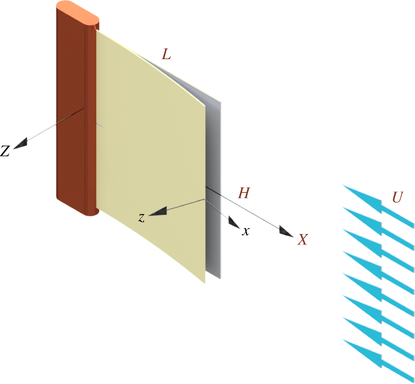
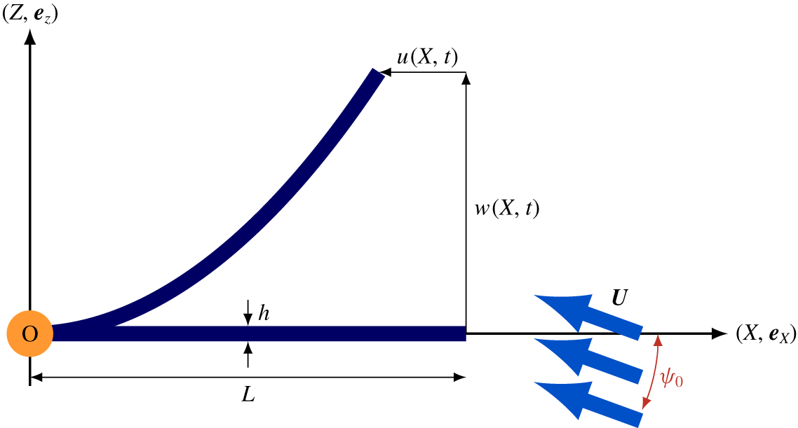
 $U$ and directed from the free end towards the clamped one, otherwise known as an ‘inverted flag’; see figure 1.
The first investigation on the dynamics and stability of inverted flags may be attributed to Guo & Païdoussis (Reference Guo and Païdoussis2000). They studied theoretically the linear stability of rectangular plates with various boundary conditions, such as clamped–free, free–free and free–clamped, in inviscid, incompressible two-dimensional (2-D) flow. They found that a free–clamped (or inverted) plate flutters via a Hopf bifurcation at a non-zero critical flow velocity which is inversely proportional to the fluid-to-plate mass ratio defined as  $\unicode[STIX]{x1D707}=\unicode[STIX]{x1D70C}_{f}L/\unicode[STIX]{x1D70C}_{p}h$;
 $\unicode[STIX]{x1D70C}_{f}$ and
 $\unicode[STIX]{x1D70C}_{p}$ being the mass density of the fluid and plate, respectively, and
 $h$ being the thickness of the plate. (Throughout the present paper, including the Introduction, the mass ratio
 $\unicode[STIX]{x1D707}$ is defined as fluid mass to structure mass. Some other authors use the inverse definition.) This differs from the divergence instability proposed by Kim et al. (Reference Kim, Cossé, Huertas Cerdeira and Gharib2013), and reported by Sader, Huertas-Cerdeira & Gharib (Reference Sader, Huertas-Cerdeira and Gharib2016b), Gurugubelli & Jaiman (Reference Gurugubelli and Jaiman2015) and Goza, Colonius & Sader (Reference Goza, Colonius and Sader2018). Recently, interest in the dynamics of inverted flags has been revived mainly due to their potential application to small-scale energy harvesting; see, for example, the experimental study by Orrego et al. (Reference Orrego, Shoele, Ruas, Doran, Caggiano, Mittal and Kang2017) on inverted piezoelectric flags. Moreover, exploring the dynamics of inverted flags is expected to improve our understanding of the flapping of biological structures, such as plant leaves in wind (Sader et al. Reference Sader, Cossé, Kim, Fan and Gharib2016a; Fan et al. Reference Fan, Huertas-Cerdeira, Cossé, Sader and Gharib2019).
Kim et al. (Reference Kim, Cossé, Huertas Cerdeira and Gharib2013) explored the dynamics of inverted flags in an open-loop wind tunnel at high Reynolds numbers  $Re\equiv UL/\unicode[STIX]{x1D708}\approx 10^{4}{-}10^{5}$,
 $\unicode[STIX]{x1D708}$ being the kinematic viscosity of the fluid. They identified three consecutive regimes/modes of dynamical behaviour, namely the stretched-straight mode, the flapping mode and the fully deflected mode, as the flow velocity in the test-section was increased. It was found that, in contrast to a typical flag, which undergoes flapping beyond a critical flow velocity, the inverted flag performs flapping only within a finite range of flow velocities, somewhat analogously to vortex-induced vibration of a spring-supported cylinder in cross-flow. It was also found that the inverted flag displays larger peak-to-peak flapping amplitude
 $A$ (up to
 $A/L=1.8$) than the conventional flag.
Following the seminal work by Kim et al. (Reference Kim, Cossé, Huertas Cerdeira and Gharib2013), several researchers employed fully computational approaches to solve the fluid–structure interaction problem of inverted flags. For example, Ryu et al. (Reference Ryu, Park, Kim and Sung2015) used the immersed boundary method (IBM) to investigate the flapping dynamics of 2-D inverted flags at relatively low Reynolds numbers (up to  $Re=250$). For
 $Re<50$, the stretched-straight and flapping modes did not arise. For
 $100\leqslant Re\leqslant 250$, however, the stretched-straight, flapping and deflected modes occurred in a regular sequence as the bending rigidity parameter of the flag, which is the reciprocal of the dimensionless flow velocity, was decreased. They found numerically that the deformation of the free end of the flag grows steadily, as the bending rigidity is decreased in the range between the stretched-straight and flapping modes. They called this intermediate regime ‘the biased mode’.
Two-dimensional inverted flag in axial flow: free at the upstream and clamped at the downstream end. The flag is assumed to be infinitely wide (i.e.  $H/L\rightarrow \infty$); hence, the fluid flow surrounding the flag is treated as two-dimensional.

Almost concurrently with Ryu et al. (Reference Ryu, Park, Kim and Sung2015), two other research groups performed computational investigations on the dynamics of inverted flags. Gilmanov, Le & Sotiropoulos (Reference Gilmanov, Le and Sotiropoulos2015) developed an FSI solver by coupling the curvilinear immersed boundary method and a free-rotation finite element model to solve systems undergoing arbitrarily large deformation. One of the case studies they considered was an inverted flag of aspect ratio  and
 $\unicode[STIX]{x1D707}\approx 0.31$ flapping in a high Reynolds number axial flow (
 $Re\sim 10^{5}$). They obtained excellent agreement with the experimental results reported by Kim et al. (Reference Kim, Cossé, Huertas Cerdeira and Gharib2013), particularly on the time history of the flag free-end displacement and the maximum and mean values of the drag coefficient. Tang, Liu & Lu (Reference Tang, Liu and Lu2015) performed computational studies on the dynamics of 3-D inverted flags in the
 $Re=100-500$ flow regime. In particular, they examined the effects of the aspect ratio of the flag and the incidence angle of the oncoming flow. For zero incidence angle, they found that, as the dimensionless flow velocity is increased (or the bending rigidity parameter is decreased) beyond the deflected mode, the flag may undergo flapping motion about the deflected shape with the free end pointing downstream. They called this behaviour the ‘deflected-flapping’ mode. They also found that, as the mass ratio or aspect ratio is increased, the flag starts flapping at a lower dimensionless flow velocity, which also persists for a wider range of flow velocities. Bistability and hysteresis are present in the range between the stretched-straight and flapping modes and between the flapping and deflected modes. For small non-zero incidence angles, they found that the flapping motion becomes asymmetric about the static equilibrium.
Shoele & Mittal (Reference Shoele and Mittal2016a) investigated interactions between a 2-D inverted piezoelectric flag and axial flow. The majority of their simulations were conducted at  $Re=200$. They found that the inverted flag is dynamically nearly insensitive to the mass ratio for the range of dimensionless flow velocities where low- or high-amplitude symmetric flapping occurs. This finding agrees with the observations made by Kim et al. (Reference Kim, Cossé, Huertas Cerdeira and Gharib2013), but contradicts the computational findings by Tang et al. (Reference Tang, Liu and Lu2015). However, it was shown that at sufficiently high flow velocities the flag bends completely, pointing downstream, and flapping becomes asymmetric. The dynamical behaviour shows a strong correlation with the mass ratio in this flow regime. In this latter configuration, in fact, the inverted flag behaves very much like a conventional flag in axial flow – where the fluid flows from the clamped end towards the free end – whose dynamical behaviour is known to be strongly dependent on the mass ratio; see, for example, Kornecki, Dowell & O’Brien (Reference Kornecki, Dowell and O’Brien1976), Connell & Yue (Reference Connell and Yue2007), Tang & Païdoussis (Reference Tang and Païdoussis2007), Eloy et al. (Reference Eloy, Lagrange, Souilliez and Schouveiler2008) and Howell et al. (Reference Howell, Lucey, Carpenter and Pitman2009). Finally, they attributed the mechanism of flapping of light flags to vortex-induced vibration (VIV) and the lock-in phenomenon.
Yu, Liu & Chen (Reference Yu, Liu and Chen2017) conducted experiments with an inverted flag in a relatively confined water channel ( $W/L=2$,
 $W$ being the width of the test-section) in the
 $Re=4660{-}7600$ flow regime. The inverted flag had an aspect ratio
 and mass ratio
 $\unicode[STIX]{x1D707}\simeq 143$. The initially straight flag buckled in the
 $Re<4940$ flow regime, becoming slightly deflected (
 $A/L<0.3$). Beyond the buckling regime, while increasing (decreasing) the Reynolds number (the dimensionless bending stiffness), three other modes were encountered: the biased mode, the flapping mode and the deflected mode. The biased mode corresponds to moderate-amplitude flapping (
 $0.3\leqslant A/L\leqslant 1.2$) about the buckled shape in the
 $5100\leqslant Re\leqslant 6000$ flow regime. The other two modes correspond, respectively, to large-amplitude flapping (
 $A/L\sim 1.8$) in the
 $6000<Re\leqslant 7122$ flow regime, and large-amplitude buckling beyond
 $Re=7400$. The flapping motion was found to undergo a hysteresis loop when the Reynolds number was decreased from
 $Re=7600$ down to
 $Re=4660$. The existence of large-amplitude flapping and deflected modes, as well as the hysteresis phenomenon, had previously been reported by Kim et al. (Reference Kim, Cossé, Huertas Cerdeira and Gharib2013).
More recently, Gurugubelli & Jaiman (Reference Gurugubelli and Jaiman2019) computationally explored the mechanism for large-amplitude flapping of 3-D inverted flags, assuming spanwise periodicity while ignoring the side-edge effects. They employed the arbitrary Lagrangian–Eulerian technique which allows the deforming mesh used for solving the fluid system to adapt to the deforming body’s Lagrangian mesh. Most simulations were conducted for a flag with  $\unicode[STIX]{x1D707}=1$ and at
 $Re=3\times 10^{4}$. In particular, they showed that flapping does not arise below a critical
 $Re$, presumably because vortex shedding does not occur in the low-
 $Re$ flow regime (
 $Re\lesssim 40$; refer to Blevins (Reference Blevins1990) and Païdoussis, Price & De Langre (Reference Païdoussis, Price and De Langre2010)). They found that the flag undergoes divergence, leading to large static deformation instead, in that flow regime. However, most recently, Goza et al. (Reference Goza, Colonius and Sader2018) showed that for sufficiently heavy flags, i.e.
 $\unicode[STIX]{x1D707}\ll 1$, large-amplitude flapping arises even for
 $Re<50$, but the mechanism of instability is not classical VIV. Gurugubelli & Jaiman (Reference Gurugubelli and Jaiman2019) also found that the aspect ratio of the flag (
 ) has a marginal effect on large-amplitude flapping. Finally, they attributed the periodic flapping motion to a complex interplay between the unsteady shedding of leading-edge vortices and the structural dynamics of the flexible flag; the trailing-edge vortices were found to have an insignificant effect on the flapping.
In an elaborate study, Sader et al. (Reference Sader, Cossé, Kim, Fan and Gharib2016a) employed a combination of mathematical theory, scaling analysis and experimental measurement to understand the underlying physical mechanism of flapping of inverted flags. They concluded that the large-amplitude flapping motion of an inverted flag is a vortex-induced vibration, in contrast to flapping of a conventional flag, which is a ‘self-excited’ oscillation. They provided some observations and analyses to support this hypothesis, e.g. that flapping occurred over the approximate range of Strouhal numbers  $St\in [0.1\,\,0.2]$ (the Strouhal number being independent of the Reynolds number) and flapping occurred above a minimum amplitude, accompanied by flow separation and periodic vortex shedding. The Strouhal number was calculated by measuring the peak-to-peak amplitude of flapping and considering the synchronization of vortex shedding and flag motion, as observed in experiments (refer also to Kim et al. (Reference Kim, Cossé, Huertas Cerdeira and Gharib2013)). Adopting steady-state aerodynamic theory in the equations obtained by Kornecki et al. (Reference Kornecki, Dowell and O’Brien1976), they showed that the onset of flapping is due to a static divergence instability and is thus independent of the mass ratio. In addition, they showed analytically (using lifting-line theory and the vortex-lattice method) and experimentally that the critical dimensionless flow velocity at which the zero-deflection equilibrium loses stability decreases as the aspect ratio is increased.
In a subsequent paper, Sader et al. (Reference Sader, Huertas-Cerdeira and Gharib2016b) examined theoretically the stability of low aspect ratio (or slender) flags and cylindrical beams (or ‘rods’ as they call them) in uniform steady axial flow. Employing the Bollay (Reference Bollay1939) quadratic normal force coefficient (i.e.  $C_{N}=2\sin ^{2}\unicode[STIX]{x1D6FC}$ for rigid, rectangular, very low aspect ratio plates,
 $\unicode[STIX]{x1D6FC}$ being the incidence angle, or angle of attack), they developed a theory to examine the static stability of slender flexible and flexibly supported rigid inverted flags. They found that at low flow velocities the zero-deflection equilibrium is the only possible stable state. However, at a critical flow velocity, a saddle-node bifurcation occurs, from which a new deflected equilibrium state emanates and grows in amplitude as the flow velocity is increased. Their experimental measurements for low aspect ratio (down to
 ) inverted flags agree well with their theoretical results, both qualitatively and quantitatively.
Sader et al. (Reference Sader, Huertas-Cerdeira and Gharib2016b) also extended the theory to the case of inverted flexible cylinders and produced some results by employing experimental system parameters in Rinaldi & Païdoussis (Reference Rinaldi and Païdoussis2012). The normal force coefficient was taken as  $C_{D}=1.1$ (Taylor Reference Taylor1952; Hoerner Reference Hoerner1965) for the theoretical calculations. They found that an inverted cylinder is stable at low flow velocities, but undergoes a saddle-node bifurcation at higher flow velocities, leading to a large-amplitude deflected equilibrium state, similarly to low aspect ratio inverted flags. This differs from Rinaldi & Païdoussis’s observations of a ‘weak’ flutter-like instability at low flow velocities, followed by divergence at higher flow velocities. Moreover, the transition from zero-deflection equilibrium to large-amplitude deflected equilibrium should normally occur abruptly, which is again different from Rinaldi & Païdoussis’s observations of a steadily growing bow with increasing flow. On the other hand, the very recent nonlinear model developed by Abdelbaki, Païdoussis & Misra (Reference Abdelbaki, Païdoussis and Misra2018) for inverted cylinders in confined axial flow corroborates qualitatively several aspects of the dynamics observed by Rinaldi & Païdoussis (Reference Rinaldi and Païdoussis2012). All of the above call for fresh experimental studies with inverted flexible cylinders. Interestingly, the theoretical predictions by Sader et al. (Reference Sader, Huertas-Cerdeira and Gharib2016b) for the saddle-node bifurcation point agree well with Rinaldi & Païdoussis’s experimental measurements of the critical flow velocity for static divergence.
In a series of studies, Tavallaeinejad, Legrand & Païdoussis (Reference Tavallaeinejad, Legrand and Païdoussis2020), Tavallaeinejad, Païdoussis & Legrand (Reference Tavallaeinejad, Païdoussis and Legrand2018) developed nonlinear theoretical models to explore the static and dynamic responses of flexible, low aspect ratio (mostly  ) inverted flags in axial flow. They used a Hamiltonian framework to derive the equations of motion. The ‘reactive’ fluid force – the fluid flow momentum change in the transverse direction due to the immersed flag’s motion – was formulated using the large-amplitude elongated body theory of Lighthill (Reference Lighthill1971), while the nonlinear or ‘vortex’ lift – due to strong vortex formation along the lateral edges of the flag (Hoerner & Borst Reference Hoerner and Borst1985) – was approximated by the nonlinear wing theory proposed by Bollay (Reference Bollay1939). They cast Bollay’s implicit equation for the normal force coefficient of a finite aspect ratio plate-like wing into a closed-form equation similar to that given by Polhamus (Reference Polhamus1966).
The nonlinear static response of the system was examined in Tavallaeinejad et al. (Reference Tavallaeinejad, Païdoussis and Legrand2018) by considering steady fluid-related forces. It was found that a low aspect ratio flag undergoes a static divergence via a subcritical pitchfork bifurcation followed by a saddle-node bifurcation. However, beyond a critical aspect ratio, the subcritical bifurcation was replaced by a supercritical bifurcation. Also, increasing the aspect ratio was found to have a destabilizing effect, which is consistent with the experimental/analytical observations of Sader et al. (Reference Sader, Cossé, Kim, Fan and Gharib2016a) and the computational results of Tang et al. (Reference Tang, Liu and Lu2015). For initially curved flags (i.e. imperfect flags), the pitchfork bifurcation was replaced by a saddle-node bifurcation. By increasing the aspect ratio, the bistable range between the two saddle-node bifurcations was progressively diminished and eventually a supercritical response appeared.
Tavallaeinejad et al. (Reference Tavallaeinejad, Legrand and Païdoussis2020) explored the nonlinear dynamics of low aspect ratio ( ), relatively heavy (
 $\unicode[STIX]{x1D707}\leqslant 0.4$) inverted flags in axial flow. For a not too slender flag, they found the following typical sequence of dynamical states, as the flow velocity is increased: (i) stable at the position of rest, (ii) flapping about the position of rest via a supercritical Hopf bifurcation (i.e. symmetric flapping mode), (iii) flapping about a deflected equilibrium (i.e. asymmetric flapping or deflected-flapping mode) via two saddle-node bifurcations and (iv) highly deflected state on one side via a Hopf bifurcation. They also found that as
 was increased from
 to
 , the behaviour changed from a fully static response (as reported in Tavallaeinejad et al. (Reference Tavallaeinejad, Païdoussis and Legrand2018)) to the complex sequence of dynamical behaviour outlined above. In addition, it was shown that the fluid flow with a non-zero incidence angle would break the symmetry of the response from essentially zero flow. Increasing the incidence angle was found to change the dynamics dramatically. At a sufficiently large incidence angle, the bistable regime vanishes altogether. Increasing the mass ratio from
 $\unicode[STIX]{x1D707}=0.1$ to
 $\unicode[STIX]{x1D707}=0.4$ was found to lower the critical flow velocity for flapping and to increase the flapping amplitude. The latter differs from the experimental observations by Kim et al. (Reference Kim, Cossé, Huertas Cerdeira and Gharib2013) (with only two data points, however) but agrees with the computational results of Tang et al. (Reference Tang, Liu and Lu2015). Finally, increasing the skin friction coefficient, approximated by boundary layer solutions (Anderson Reference Anderson2017), was found to lower the critical flow velocities for the secondary bifurcations, as well as the flapping amplitude.
Finally, inspired by the planform of tree leaves, Fan et al. (Reference Fan, Huertas-Cerdeira, Cossé, Sader and Gharib2019) explored the effects of the plan-view shape of the inverted flag on its stability and dynamics. Wind tunnel tests were carried out with trapezoidal sheets of  , taper ratio
 $0\leqslant \unicode[STIX]{x1D6E5}/H\leqslant 1.75$ (
 $\unicode[STIX]{x1D6E5}$ and
 $H$ being the height at the free and clamped ends, respectively) and two different thicknesses, yielding
 $\unicode[STIX]{x1D707}=0.40$ and
 $\unicode[STIX]{x1D707}=0.61$ (presumably for the rectangular sheets), in
 $Re\approx 10^{4}-10^{5}$ flow. They found that, as the taper ratio (or shape parameter)
 $\unicode[STIX]{x1D6E5}/H$ is increased, the critical flow velocities for both the onset and cessation of flapping and the flow speed range over which flapping occurs decrease. Interestingly, the ratio of the two critical flow velocities (i.e. cessation to onset) for all trapezoidal shapes tested was found to be approximately
 $4$. In addition, they developed an extended form of the analytical model developed in Sader et al. (Reference Sader, Cossé, Kim, Fan and Gharib2016a) for predicting the divergence instability of an inverted flag of arbitrary shape, and good agreement with experimental results was achieved. Moreover, they studied experimentally and analytically a new configuration of inverted flags, where a rectangular sheet is attached to a slender elastic strip (to mimic a ‘petiole’ or the stalk that attaches the leaf to the stem) which is clamped at its other end. Similar global dynamical behaviour as for the flag with no petiole was observed, namely: undeflected equilibrium, flapping and deflected equilibrium. It was also reported that it is the petiole which provides the primary source of elasticity, while the elastic sheet undergoes rigid-body motion.
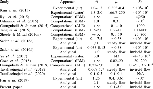
A summary and taxonomy of previous studies is presented in table 1. This table strictly aims at reporting the range of system parameters investigated in each study and does not assess the validity of their findings. The present paper explores the effect of mass ratio for  $\unicode[STIX]{x1D707}\in [0.1\,\,5.0]$, but the results may not match all features present in the experiments of Kim et al. (Reference Kim, Cossé, Huertas Cerdeira and Gharib2013).
Taxonomy of recent studies on inverted flags. IBM and ALE are the abbreviations for ‘immersed boundary method’ and ‘arbitrary Lagrangian–Eulerian’ scheme, respectively; N/A stands for ‘not applicable’.

The aim of the present paper is to investigate analytically the nonlinear dynamics and post-critical behaviour of inverted flags in axial flow. In particular, we aim at deriving an analytical model for the dynamics of high aspect ratio, heavy inverted flags by leveraging inviscid flow aerodynamic theory. Despite recent advances in computational fluid dynamics methods, which make them practically viable for use in fully coupled fluid–structure interaction solvers, analytical approaches are still attractive for solving complex FSI problems. Analytical solutions are obtained in a faster fashion and thus are superior for parametric studies to, for example, computational models based on direct numerical simulation (DNS) or large-eddy simulation (LES) of the fluid flow. Moreover, analytical models often give valuable insight into the underlying mechanisms of the dynamics of the system.
Thus, a continuum analytical representation of fluid forces is obtained and detailed based on the quasi-steady version of the unsteady aerodynamic theory of Theodorsen (Reference Theodorsen1949) to formulate the reactive force, and the leading-edge suction analogy of Polhamus (Reference Polhamus1966) to deal with the separated flow at the flag leading edge, with no account taken of periodicity of fluid dynamic forces due to leading-edge vortex shedding. The analytical model will be used to predict, for example, the onset of instabilities, frequency and amplitude of flapping, as well as the physical mechanisms involved in the transition from one regime to another.
The rest of the paper is organized as follows. In § 2, the extended Hamilton’s principle is employed to derive the equations of motion from the kinetic and potential energies of the system, as well as the virtual work due to fluid-related forces. The resulting partial-integro-differential equations are then discretized spatially by means of the Galerkin method and they are recast as a set of nonlinear ordinary differential equations. In § 3, the linearized form of the equations of motion is obtained, and the linear dynamics of the system is explored by solving an eigenvalue problem. The nonlinear response of the system is examined in detail in § 4, by utilizing direct time integration and bifurcation analysis. The sensitivity of the dynamics to the mass ratio and the angle of attack is also explored. The results are summarized in the form of bifurcation diagrams to identify the transition between various regimes. It is shown that lighter flags are more likely to exhibit hysteresis in their dynamical response. In § 5, the effectiveness of the model is demonstrated by comparing the obtained results with those available in the literature, highlighting that the proposed model captures both the qualitative behaviour and the detailed dynamics observed in previous studies.
2 Analytical modelling
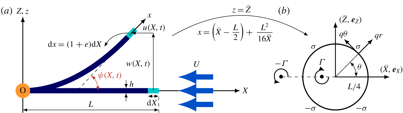
In this section, a nonlinear model is developed for the inverted flag problem. First, the inverted flag problem is defined mathematically. The kinetic and potential energies of the inverted flag, idealized as a cantilevered elastic beam, as shown in figure 2, are derived according to the nonlinear Euler–Bernoulli beam theory. Next, expressions for fluid forces are formulated separately, and the associated virtual work is derived. Finally, the nonlinear integro-partial-differential equations governing the rotation of the mid-plane are derived via the extended Hamilton’s principle. These equations are non-dimensionalized and then discretized via the Galerkin method.
2.1 Definitions and preliminaries
The system under consideration is shown schematically in figure 1, consisting of a vertical cantilevered thin plate subjected to an inviscid axial flow impinging on its free end. The flag is assumed to be infinitely wide (i.e.  ); hence, the fluid flow surrounding the flag is treated as being two-dimensional. The spanwise variation of the fluid-related loads is neglected; the flag is therefore idealized as a cantilevered Euler–Bernoulli beam. The inverted flag is of infinite span, finite chord
 $L$, thickness
 $h$ and flexural rigidity
 $D$. The mechanical properties of the flag, i.e. the mass density, Poisson ratio, Young’s modulus and internal damping coefficient are represented by
 $\unicode[STIX]{x1D70C}_{p}$,
 $\unicode[STIX]{x1D708}_{p}$,
 $E$ and
 $\unicode[STIX]{x1D702}$, respectively;
 $\unicode[STIX]{x1D70C}_{f}$ stands for the density of the fluid flowing with mean flow velocity
 $U$. Two coordinate systems are defined: (i) a right-handed rectangular Cartesian reference system
 $(O;XZ)$, with the
 $X(\boldsymbol{e}_{X})$ and
 $Z(\boldsymbol{e}_{Z})$ axes being in the axial and transverse directions, respectively; (ii) a curvilinear coordinate system
 $(O;xz)$, with the
 $x$-axis being along the flag centreline from its clamped end towards the free one. The unit vectors
 $\boldsymbol{e}_{x}$ and
 $\boldsymbol{e}_{z}$ are tangential and normal to the centreline, respectively.
(a) The flag is idealized as an inextensible (i.e.  $e=0$) cantilevered beam. An arbitrary infinitesimal element
 $\text{d}x$ of the beam undergoes longitudinal
 $u(X,t)$ and transverse
 $w(X,t)$ displacements, related to each other by the rotation angle
 $\unicode[STIX]{x1D713}(X,t)$. (b) Joukowski’s conformal mapping of the plate into a circle of radius
 $L/4$ (i.e.
 $\bar{X}\bar{Z}$-plane);
 $q_{r}$ and
 $q_{\unicode[STIX]{x1D703}}$ are the radial and circumferential velocities on the circle in the
 $\bar{X}\bar{Z}$-plane, respectively. The impermeability condition is satisfied by considering a set of sources and sinks of strength
 $\unicode[STIX]{x1D70E}$ on the top and bottom halves of the circle, respectively. The induced velocity due to a single bound vortex of strength
 $\unicode[STIX]{x1D6E4}$ and its image (i.e. the wake vortex of strength
 $-\unicode[STIX]{x1D6E4}$) at an arbitrary point on the circle satisfies the Kutta condition.

The rotation angle  $\unicode[STIX]{x1D713}(X,t)$, the curvature
 $\unicode[STIX]{x1D705}(X,t)$ and the axial strain
 $e(X,t)$ are related to the longitudinal and transverse motions,
 $u(X,t)$ and
 $w(X,t)$ respectively, of a generic point at a distance
 $Z$ from the mid-plane on the cross-section, by
 $$\begin{eqnarray}\sin \unicode[STIX]{x1D713}(X,t)=\frac{\unicode[STIX]{x2202}_{X}w(X,t)}{1+e(X,t)},\quad \cos \unicode[STIX]{x1D713}(X,t)=\frac{1+\unicode[STIX]{x2202}_{X}u(X,t)}{1+e(X,t)},\quad \unicode[STIX]{x1D705}(X,t)=\frac{\unicode[STIX]{x2202}_{X}\unicode[STIX]{x1D713}(x,t)}{1+e(X,t)},\end{eqnarray}$$
where  $\unicode[STIX]{x2202}_{X}\equiv \unicode[STIX]{x2202}/\unicode[STIX]{x2202}X$ denotes the first spatial derivative. In the remainder of this paper,
 $\unicode[STIX]{x2202}_{\bullet }$ is defined as the first derivative with respect to
 $\bullet$,
 $\unicode[STIX]{x2202}_{\bullet \bullet }$ denotes the second derivative, and so on. The inextensibility assumption reads
 $e(X,t)=0$, which yields
 $(1+\unicode[STIX]{x2202}_{X}u(X,t))^{2}+(\unicode[STIX]{x2202}_{X}w(X,t))^{2}=1$ (Farokhi, Païdoussis & Misra Reference Farokhi, Païdoussis and Misra2018), indicating that the length of the flag centreline remains constant during vibrations. This condition allows us to express all physical quantities in terms of the curvilinear coordinate
 $(x,t)$ (refer to Nayfeh & Pai (Reference Nayfeh and Pai2008) or Lopes, Païdoussis & Semler (Reference Lopes, Païdoussis and Semler2002)). Additionally, it reduces the dependent variables to one, and
 $w(x,t)$ and
 $u(x,t)$ may be expressed in terms of the rotation angle of the cross-section
 $\unicode[STIX]{x1D713}(x,t)$. Hence, velocity components of an element may be formulated as
 $$\begin{eqnarray}\left.\begin{array}{@{}c@{}}\displaystyle {\dot{w}}(x,t)=\int _{0}^{s}\dot{\unicode[STIX]{x1D713}}(s,t)\cos \unicode[STIX]{x1D713}(s,t)\,\text{d}s,\\ \displaystyle \dot{u}(x,t)=-\int _{0}^{s}\dot{\unicode[STIX]{x1D713}}(s,t)\sin \unicode[STIX]{x1D713}(s,t)\,\text{d}s,\end{array}\right\}\end{eqnarray}$$
where the overdot denotes the derivative with respect to time.
Considering a set of longitudinal and transverse displacements (i.e.  $u(x,t)$ and
 $w(x,t)$, respectively) of the element
 $\text{d}x$ shown in figure 2, away from its undeflected static equilibrium, the relative velocity between the structure and the incident flow in the tangential and normal directions may be written as
 $$\begin{eqnarray}\displaystyle \boldsymbol{V}_{rel}(x,t) & = & \displaystyle V_{\unicode[STIX]{x1D70F}}(x,t)\boldsymbol{e}_{x}+V_{n}(x,t)\boldsymbol{e}_{z}\nonumber\\ \displaystyle & = & \displaystyle [(\dot{u}+U)\cos \unicode[STIX]{x1D713}+{\dot{w}}\sin \unicode[STIX]{x1D713}]\boldsymbol{e}_{x}+[-(\dot{u}+U)\sin \unicode[STIX]{x1D713}+{\dot{w}}\cos \unicode[STIX]{x1D713}]\boldsymbol{e}_{z}.\end{eqnarray}$$
In this paper, the governing equations are derived in a Hamiltonian framework. The extended Hamilton’s principle may be expressed as
 $$\begin{eqnarray}\int _{t_{1}}^{t_{2}}(\unicode[STIX]{x1D6FF}{\mathcal{T}}(t)-\unicode[STIX]{x1D6FF}{\mathcal{V}}(t)+\unicode[STIX]{x1D6FF}{\mathcal{W}}_{f}(t)+\unicode[STIX]{x1D6FF}{\mathcal{W}}_{d}(t))\,\text{d}t=0,\end{eqnarray}$$
with  ${\mathcal{T}}(t)$ and
 ${\mathcal{V}}(t)$ denoting the kinetic and potential energies of the system, respectively, and
 $\unicode[STIX]{x1D6FF}{\mathcal{W}}_{f}(t)$ and
 $\unicode[STIX]{x1D6FF}{\mathcal{W}}_{d}(t)$ the virtual work by the fluid forces acting on the inverted flag and damping, respectively; here
 $\unicode[STIX]{x1D6FF}$ denotes the variational operator.
2.2 Kinetic and potential energies
In this study, the centreline rotation of the inverted flag  $\unicode[STIX]{x1D713}(x,t)$, is taken as the primary variable for describing the flag motion. This can be achieved with the aid of (2.1) and taking into account the inextensibility assumption. Derivation of the equation of motion in terms of the rotation angle allows prediction of large-amplitude deformations even when the tip rotation exceeds
 $\unicode[STIX]{x03C0}/2$ (refer to Tavallaeinejad et al. (Reference Tavallaeinejad, Païdoussis and Legrand2018)). Thus, in what follows, the kinetic and potential energies as well as the virtual work of fluid-related forces and damping are formulated as functions of
 $\unicode[STIX]{x1D713}(x,t)$.
The kinetic energy of the system for translational and rotational motions of the inverted flag may be written as
 $$\begin{eqnarray}\displaystyle {\mathcal{T}}(t) & = & \displaystyle {\textstyle \frac{1}{2}}\unicode[STIX]{x1D70C}_{p}h\int _{0}^{L}\left[\left(\int _{0}^{x}\sin \unicode[STIX]{x1D713}(s,t)\dot{\unicode[STIX]{x1D713}}(s,t)\,\text{d}s\right)^{2}+\left(\int _{0}^{x}\cos \unicode[STIX]{x1D713}(s,t)\dot{\unicode[STIX]{x1D713}}(s,t)\,\text{d}s\right)^{2}\right]\,\text{d}x\nonumber\\ \displaystyle & & \displaystyle +\,{\textstyle \frac{1}{24}}\unicode[STIX]{x1D70C}_{p}h^{3}\int _{0}^{L}\dot{\unicode[STIX]{x1D713}}(x,t)^{2}\,\text{d}x.\end{eqnarray}$$
The potential strain energy of the inextensible inverted flag in terms of the rotation angle is
 $$\begin{eqnarray}{\mathcal{V}}(t)={\textstyle \frac{1}{2}}D\int _{0}^{L}(\unicode[STIX]{x2202}_{x}\unicode[STIX]{x1D713}(x,t))^{2}\,\text{d}x,\end{eqnarray}$$
in which  $D=Eh^{3}/(12(1-\unicode[STIX]{x1D708}_{p}^{2}))$ is the plane-strain flexural rigidity for plates of large aspect ratio. The virtual work done by the Kelvin–Voigt structural damping may be formulated as
 $$\begin{eqnarray}\unicode[STIX]{x1D6FF}{\mathcal{W}}_{d}(t)=-D\unicode[STIX]{x1D702}\int _{0}^{L}\unicode[STIX]{x2202}_{xx}\dot{\unicode[STIX]{x1D713}}(x,t)\unicode[STIX]{x1D6FF}\unicode[STIX]{x1D713}\,\text{d}x,\end{eqnarray}$$
where  $\unicode[STIX]{x1D702}$ denotes the viscoelastic damping coefficient. Material damping is introduced in the model since it is an inherent property of all materials; it provides a means to model the dissipation of the energy pumped into the flag from the fluid flow. The structural damping model utilized in the proposed model is more appropriate than a generic linear viscous damping model. The virtual work done by the fluid-related force normal to the flag is given by
 $$\begin{eqnarray}\unicode[STIX]{x1D6FF}{\mathcal{W}}_{F}(t)=\int _{0}^{L}(F_{N}(x,t)\cos \unicode[STIX]{x1D713}(x,t)\unicode[STIX]{x1D6FF}w-F_{N}(x,t)\sin \unicode[STIX]{x1D713}(x,t)\unicode[STIX]{x1D6FF}u)\,\text{d}x,\end{eqnarray}$$
in which  $F_{N}$ represents the normal force acting on the flag, and is derived in the following section.
2.3 Aerodynamic model
The inviscid pressure-related forces are modelled in this section. The flow is assumed to be inviscid and two-dimensional around a thin flat plate. The 2-D quasi-steady thin airfoil theory, involving large angles of attack, is employed to formulate the reactive fluid forces corresponding to the relative motion of the inverted flag with respect to the incident flow; for details the reader is referred to Bisplinghoff, Ashley & Halfman (Reference Bisplinghoff, Ashley and Halfman2013), Ramesh et al. (Reference Ramesh, Gopalarathnam, Edwards, Ol and Granlund2013) and Yan, Taha & Hajj (Reference Yan, Taha and Hajj2014). The influence of leading-edge separation is dealt with separately. First, the quasi-steady forces are derived using a velocity potential approach in a way that the solution is divided into non-circulatory and circulatory contributions; each part is obtained using a Joukowski conformal transformation. Next, the separated flow at the leading edge is modelled utilizing the leading edge suction analogy of Polhamus (Reference Polhamus1966).
We consider a two-dimensional perturbation velocity potential due to the motion of the plate  $\unicode[STIX]{x1D719}(x,z,t)$, which satisfies the Laplace equation (i.e.
 $\unicode[STIX]{x1D6FB}^{2}\unicode[STIX]{x1D719}=0$, with
 $\unicode[STIX]{x1D735}$ being a first-order spatial differential operator). Following Theodorsen’s approach, the perturbation velocity potential may be divided into two parts:
 $\unicode[STIX]{x1D719}=\unicode[STIX]{x1D719}^{nc}+\unicode[STIX]{x1D719}^{c}$, where
 $\unicode[STIX]{x1D719}^{c}$ is the circulatory component, fulfilling the Kutta condition, and
 $\unicode[STIX]{x1D719}^{nc}$ denotes the non-circulatory component which satisfies the impermeability condition.
The pressure difference between the lower and upper surfaces may be formulated using the unsteady Bernoulli equation (refer to Ramesh et al. (Reference Ramesh, Gopalarathnam, Edwards, Ol and Granlund2013) and Yan et al. (Reference Yan, Taha and Hajj2014)),
 $$\begin{eqnarray}\unicode[STIX]{x0394}P(x,t)=P_{u}(x,t)-P_{l}(x,t)=-2\unicode[STIX]{x1D70C}[\dot{\unicode[STIX]{x1D719}}_{u}-((\dot{u}+U)\cos \unicode[STIX]{x1D713}+{\dot{w}}\sin \unicode[STIX]{x1D713})\unicode[STIX]{x2202}_{x}\unicode[STIX]{x1D719}_{u}].\end{eqnarray}$$
Following Theodorsen’s approach, the pressure difference over the flag is decomposed into two contributions, namely non-circulatory and circulatory components. Hence, the total pressure may be written as
 $$\begin{eqnarray}\unicode[STIX]{x0394}P(x,t)=\unicode[STIX]{x0394}P^{nc}(x,t)+\unicode[STIX]{x0394}P^{c}(x,t).\end{eqnarray}$$
The non-circulatory (or added mass) component, represented by  $\unicode[STIX]{x0394}P^{nc}(x,t)$, contributes to the perturbation pressure due to the displacement of the surrounding fluid (Bisplinghoff et al. Reference Bisplinghoff, Ashley and Halfman2013). The circulatory contribution (vortex-induced pressure), denoted by
 $\unicode[STIX]{x0394}P^{c}(x,t)$, on the other hand, dominates the perturbation pressure in the vicinity of the trailing edge due to shedding of vorticity (Staubli & Rockwell Reference Staubli and Rockwell1989).
2.3.1 Non-circulatory contribution
In order to find the solution of the two-dimensional incompressible potential flow, the plate is mapped into a circle with its centre at the origin and radius  $r=L/4$, through the following standard conformal mapping illustrated in figure 2:
 $$\begin{eqnarray}x+\text{i}z=\bar{X}+\frac{L}{2}+\text{i}\bar{Z}+\frac{L^{2}}{16(\bar{X}+\text{i}\bar{Z})}.\end{eqnarray}$$
Given that  $\bar{X}=L/(4\cos \unicode[STIX]{x1D703})$ and
 $\bar{Z}=L/(4\sin \unicode[STIX]{x1D703})$, the relation between points on the flag and the circle may be found using (2.11) as
 $x=(1+\cos \unicode[STIX]{x1D703})/2$.
Considering a continuous distribution of source–sink of strengths  $\unicode[STIX]{x1D70E}(\unicode[STIX]{x1D703},t)$ and
 $-\unicode[STIX]{x1D70E}(\unicode[STIX]{x1D703},t)$ over the upper and lower surfaces of the sheet (or on its circle counterpart in figure 2), which satisfies the impermeability boundary condition, and after several manipulations, the strength per unit length of the source sheet can be found as
 $\unicode[STIX]{x1D70E}(\unicode[STIX]{x1D703},t)=4V_{n}(\unicode[STIX]{x1D703},t)\sin \unicode[STIX]{x1D703}$ (refer to Bisplinghoff et al. (Reference Bisplinghoff, Ashley and Halfman2013)). Considering an infinitesimal element of the source sheet
 $(L/4)\,\text{d}\unicode[STIX]{x1D711}$ on the circle at
 $\unicode[STIX]{x1D703}=\unicode[STIX]{x1D711}$, along with its sink counterpart at
 $\unicode[STIX]{x1D703}=-\unicode[STIX]{x1D711}$, and integrating over the half-circle, the non-circulatory component of the resultant tangential velocity may be formulated as
 $$\begin{eqnarray}q_{\unicode[STIX]{x1D703}}^{nc}(\unicode[STIX]{x1D703},t)=\frac{2}{\unicode[STIX]{x03C0}}\int _{0}^{\unicode[STIX]{x03C0}}V_{n}(\unicode[STIX]{x1D711},t)\frac{\sin ^{2}\unicode[STIX]{x1D711}}{\cos \unicode[STIX]{x1D711}-\cos \unicode[STIX]{x1D703}}\,\text{d}\unicode[STIX]{x1D711}.\end{eqnarray}$$
Assuming that  $\unicode[STIX]{x1D719}_{u}^{nc}(L/4,0,t)=0$ at the leading edge (i.e.
 $\unicode[STIX]{x1D703}=0$), the non-circulatory perturbation velocity potential in the
 $\bar{X}\bar{Z}$ plane at
 $r=L/4$ may be found,
 $$\begin{eqnarray}\unicode[STIX]{x1D719}_{u}^{nc}(\unicode[STIX]{x1D703},t)=-\frac{L}{2\unicode[STIX]{x03C0}}\int _{\unicode[STIX]{x1D703}}^{0}\int _{0}^{\unicode[STIX]{x03C0}}\frac{V_{n}(\unicode[STIX]{x1D711},t)\sin ^{2}\unicode[STIX]{x1D711}}{\cos \unicode[STIX]{x1D711}-\cos \unicode[STIX]{x1D717}}\,\text{d}\unicode[STIX]{x1D711}\,\text{d}\unicode[STIX]{x1D717}.\end{eqnarray}$$
Substitution of (2.13) into (2.9), changing the variables by making use of  $x=(1+\cos \unicode[STIX]{x1D703})/2$ and using the chain rule, the pressure distribution over the flag due to the non-circulatory contribution of the flow in the
 $\bar{X}\bar{Z}$ plane at
 $r=L/4$ may be written as
 $$\begin{eqnarray}\displaystyle \unicode[STIX]{x0394}P^{nc}(\unicode[STIX]{x1D703},t) & = & \displaystyle -\unicode[STIX]{x1D70C}\left[\frac{L}{2}\unicode[STIX]{x2202}_{t}\left(\int _{\unicode[STIX]{x1D703}}^{0}\int _{0}^{\unicode[STIX]{x03C0}}\frac{V_{n}(\unicode[STIX]{x1D711},t)\sin ^{2}\unicode[STIX]{x1D711}}{\cos \unicode[STIX]{x1D711}-\cos \unicode[STIX]{x1D717}}\,\text{d}\unicode[STIX]{x1D711}\,\text{d}\unicode[STIX]{x1D717}\right)\right.\nonumber\\ \displaystyle & & \displaystyle -\left.\frac{1}{\sin \unicode[STIX]{x1D703}}((\dot{u}+U)\cos \unicode[STIX]{x1D713}+{\dot{w}}\sin \unicode[STIX]{x1D713})\int _{0}^{\unicode[STIX]{x03C0}}\frac{V_{n}(\unicode[STIX]{x1D711},t)\sin ^{2}\unicode[STIX]{x1D711}}{\cos \unicode[STIX]{x1D711}-\cos \unicode[STIX]{x1D703}}\,\text{d}\unicode[STIX]{x1D711}\right].\qquad\end{eqnarray}$$
2.3.2 Circulatory contribution
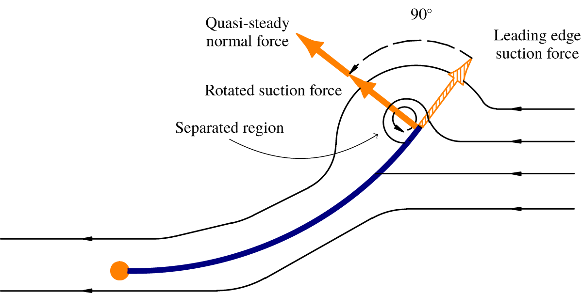
The Kutta condition enforces that the flow leaves smoothly the trailing edge of the inverted flag and hence avoids an infinite velocity at the trailing edge (i.e.  $\unicode[STIX]{x1D703}=\unicode[STIX]{x03C0}$); see figure 3. It is known that the non-circulatory solution by itself is unable to satisfy the Kutta condition. Theodorsen (Reference Theodorsen1949) fulfilled the condition by considering bound vortices, along with a wake of counter-vortices continuously shedding from the trailing edge at the free-stream velocity. The induced velocity due to the bound vortices and their ‘images’ cancels the tangential velocity at the trailing edge due to the non-circulatory component of the flow. Hence,
 $$\begin{eqnarray}q_{\unicode[STIX]{x1D703}}^{nc}(L/4,\unicode[STIX]{x1D703}=\unicode[STIX]{x03C0},t)+q_{\unicode[STIX]{x1D703}}^{c}(L/4,\unicode[STIX]{x1D703}=\unicode[STIX]{x03C0},t)=0.\end{eqnarray}$$
Subsequently, Theodorsen obtained the induced velocity due to a single bound vortex of strength  $\unicode[STIX]{x1D6E4}$ and its image (i.e. the wake vortex of strength
 $-\unicode[STIX]{x1D6E4}$) at an arbitrary point on the circle and formulated the circulatory component of the tangential velocity as
 $$\begin{eqnarray}q_{\unicode[STIX]{x1D703}}^{c}(\unicode[STIX]{x1D703},\bar{X},t)=-\frac{\unicode[STIX]{x1D6E4}}{2\unicode[STIX]{x03C0}}\left(\frac{\bar{X}^{2}-L^{2}/4}{\bar{X}^{2}+L^{2}/4+\bar{X}(L/2)\cos \unicode[STIX]{x1D703}}\right).\end{eqnarray}$$
Applying the Kutta condition at the trailing edge (i.e.  $\unicode[STIX]{x1D703}=\unicode[STIX]{x03C0}$) and the quasi-steady assumption, which neglects only the influence of the wake vortices on the flow (refer to Bisplinghoff et al. (Reference Bisplinghoff, Ashley and Halfman2013)), the pressure distribution originating from the circulatory contribution of the flow may be written as
 $$\begin{eqnarray}\unicode[STIX]{x0394}P^{c}(\unicode[STIX]{x1D703},t)=-2\unicode[STIX]{x1D70C}\left(-\dot{\unicode[STIX]{x1D719}}_{u}^{c}(\unicode[STIX]{x1D703},t)+\frac{2V_{\unicode[STIX]{x1D70F}}}{L\sin \unicode[STIX]{x1D703}}\unicode[STIX]{x2202}_{\unicode[STIX]{x1D703}}\unicode[STIX]{x1D719}_{u}^{c}(\unicode[STIX]{x1D703},t)\right)=-\frac{\unicode[STIX]{x1D70C}V_{\unicode[STIX]{x1D70F}}q_{\unicode[STIX]{x1D703}}^{nc}(\unicode[STIX]{x03C0},t)}{\sin \unicode[STIX]{x1D703}}.\end{eqnarray}$$
To see the full derivation, the interested reader is referred to Bisplinghoff et al. (Reference Bisplinghoff, Ashley and Halfman2013). The quasi-steady assumption is an approximation of Theodorsen’s theory, in which  $C(k)\rightarrow 1$, with
 $C(k)$ being Theodorsen’s function based on Hankel functions of the second kind, with
 $k$ denoting the reduced frequency. The quasi-steady theory can be used in the time domain for slow harmonic oscillations with small
 $k$, or slowly varying motion that is not harmonic (Hodges & Pierce Reference Hodges and Pierce2011). It ought to be noted that expression (2.17) ignores the effects of flow history in the wake behind the trailing edge, and instead considers the forces generated by the instantaneous deformation, velocity and acceleration of the flag; the rationale for this is detailed in the following.
Direct numerical simulations by Gurugubelli & Jaiman (Reference Gurugubelli and Jaiman2019) for an inverted flag with a splitter plate at the trailing edge reveal that, despite the total suppression of vortex shedding from the trailing edge, the large-amplitude flapping persists, with only a minor change in the frequency and amplitude of the oscillations. This suggests that the large-amplitude flapping of inverted flags may not require wake–flag synchronization. In other words, the effect of wake flow unsteadiness on the dynamical behaviour of the system seems to be insignificant, suggesting that a quasi-steady modelling of fluid forces may be acceptable.
Flow around the 2-D inverted flag placed in an inviscid fluid. The Kutta condition enforces a smooth, tangential flow leaving the trailing edge. However, according to Polhamus’ leading-edge suction analogy, the leading-edge suction vanishes due to separation at the leading edge, and it forms a leading-edge vortex. This results in a normal force component of equal magnitude to the leading-edge suction. Effectively, the leading-edge suction force is rotated by  $90^{\circ }$ onto the low-pressure side of the flag.

Nevertheless, future work ought to employ a nonlinear analytical model accounting for the unsteady wake function (in the time domain) behind the trailing edge, to further investigate the global dynamical behaviour of the inverted flag system; this is not a trivial task and it is beyond the scope of this paper.
2.3.3 Leading-edge suction force
The 2-D quasi-steady aerodynamic model employed in this paper is based on inviscid potential flow theory which, by definition, ignores any viscous effects such as flow separation or viscous stresses acting on the inverted flag. Accounting for the effects of flow separation from the leading edge is of particular importance for modelling the dynamics of inverted flags. As observed by Yu et al. (Reference Yu, Liu and Chen2017), the flow separates from the leading edge, giving rise to a stable attached vortex above the leading edge up to the angle of attack of about  $22^{\circ }$, and a normal force stall at larger angles of attack where reattachment fails to occur. The leading-edge flow separation reduces the pressure over the upper surface of the plate and its impact becomes typically stronger at high incidence angles on thin sharp-edged plates. In fact, potential flow theories alone tend to underestimate the normal force for thin sharp-edged plates at high angles, and they need to be modified either by employing analytical models, such as the Polhamus suction analogy, or by employing fully numerical schemes to model the actual flow field.
In the present work, in order to account for the effects of the leading-edge vortices, the nonlinear vortex force associated with the separated flow from the leading edge is formulated via the Polhamus analogy (Polhamus Reference Polhamus1966) as a correction to the quasi-steady pressure derived earlier. This model formulates a nonlinear relation between the potential force and the angle of attack, which acts normal to the flag, and thus modifies the normal force, as shown in figure 3. Thus, the effect of leading-edge vortices can be taken into account via superimposing linearly the nonlinear vortex lift and the quasi-steady forces due to the attached flow (Sane Reference Sane2003). A more comprehensive approach may be to determine all contributions together, via a direct utilization of the Navier–Stokes equations, for instance. The approach employed here simplifies the analysis considerably and has been shown to give acceptable results for a wide range of problems; for example, refer to the work of Pedersen & Żbikowski (Reference Pedersen and Żbikowski2006) on insect-like flapping wings in hover and Azuma & Okamoto (Reference Azuma and Okamoto2005) on deflected wings, among others.
In order to implement the method outlined above, the leading-edge suction needs to be expressed in terms of the quasi-steady force obtained earlier. Hence, the Blasius formula (Yan et al. Reference Yan, Taha and Hajj2014) is employed to determine the leading-edge suction. Integration of the pressure around a contour at the leading edge, and application of Bernoulli’s equation yields
 $$\begin{eqnarray}F_{x}-\text{i}F_{z}=-\frac{\text{i}\unicode[STIX]{x1D70C}L}{4}\int _{LE}\left(\frac{q_{\bar{X}}-\text{i}q_{\bar{Z}}}{1-2e^{-\text{i}\unicode[STIX]{x1D703}}}\right)^{2}\sin \unicode[STIX]{x1D703}\,\text{d}\unicode[STIX]{x1D703},\end{eqnarray}$$
where  $F_{x}$ and
 $F_{z}$ represent the aerodynamic forces acting on an immersed body. Assuming that the contribution of the non-circulatory component in the induced velocity near the leading edge outweighs the other contributions and recalling that
 $q_{\bar{X}}=-q_{\unicode[STIX]{x1D703}}^{nc}\sin \unicode[STIX]{x1D703}$ and
 $q_{\bar{Z}}=q_{\unicode[STIX]{x1D703}}^{nc}\cos \unicode[STIX]{x1D703}$, the leading-edge suction force at
 $r=L/4$ is
 $$\begin{eqnarray}F_{p}(t)=\frac{\unicode[STIX]{x03C0}\unicode[STIX]{x1D70C}L}{16}(q_{\unicode[STIX]{x1D703}}^{nc}(0,t))^{2}.\end{eqnarray}$$
Although the suction analogy does not model the actual flow field, it has been shown to be remarkably accurate, especially at high angles of incidence. For instance, this model has been used successfully in predicting the nonlinear vortex lift of delta wings (Purvis Reference Purvis1981; DeVoria & Mohseni Reference DeVoria and Mohseni2017) and in the theoretical modelling of flapping flight of insects (Pedersen & Żbikowski Reference Pedersen and Żbikowski2006).
It ought to be emphasized that the leading-edge suction model used in the present paper fails to include the effects of vortex shedding from the leading edge. Thus, the time-variant fluid forces acting on the flag model may not be truly representative of those in reality, which in turn may result in inaccurate predictions of the dynamical behaviour (stability, amplitude and frequency of oscillations). Nevertheless, how the vortex-shedding load affects both the local and global dynamics of the flag is not yet known and is yet to be understood. Accounting for such a load in the analytical model is a very challenging task and is not attempted in this paper.
2.3.4 Total aerodynamic force
As mentioned in the last section, the nonlinear vortex lift can be superimposed linearly on the quasi-steady pressure. Hence, the total quasi-steady normal force acting on the inverted flag is obtained as
 $$\begin{eqnarray}F_{N}(\unicode[STIX]{x1D703},t)=-\unicode[STIX]{x0394}P(\unicode[STIX]{x1D703},t)-2F_{p}(t)\,\unicode[STIX]{x1D6FF}_{D}(\cos \unicode[STIX]{x1D703}-1),\end{eqnarray}$$
with the total quasi-steady pressure formulated as
 $$\begin{eqnarray}\unicode[STIX]{x0394}P(\unicode[STIX]{x1D703},t)=\unicode[STIX]{x1D70C}\left[\frac{L}{2}\unicode[STIX]{x2202}_{t}\left(\int _{0}^{\unicode[STIX]{x1D703}}q_{\unicode[STIX]{x1D703}}^{nc}(\unicode[STIX]{x1D717},t)\,\text{d}\unicode[STIX]{x1D717}\right)+\frac{V_{\unicode[STIX]{x1D70F}}}{\sin \unicode[STIX]{x1D703}}(q_{\unicode[STIX]{x1D703}}^{nc}(\unicode[STIX]{x1D703},t)-q_{\unicode[STIX]{x1D703}}^{nc}(\unicode[STIX]{x03C0},t))\right],\end{eqnarray}$$
where  $\unicode[STIX]{x1D6FF}_{D}(x-L)$ denotes the Dirac delta function. It is noted that dealing with a non-homogenous, non-classical boundary condition is a more challenging task; hence, the end shear due to the force that results from the Polhamus effect at the leading edge is transferred from the boundary condition into the equation of motion via the Dirac delta function.
Substituting (2.21) into (2.8) and recalling that  $x=(1+\cos \unicode[STIX]{x1D703})/2$ yields the virtual work done by the fluid-related force normal to the flag.
2.4 Equation of motion
Substituting equations (2.5)–(2.8) into the generalized Hamilton’s principle given in (2.4) and performing integration by parts yields the nonlinear governing equation of motion in terms of the rotation angle  $\unicode[STIX]{x1D713}(x,t)$:
 $$\begin{eqnarray}\displaystyle & & \displaystyle {\textstyle \frac{1}{12}}\unicode[STIX]{x1D70C}_{p}h^{3}\ddot{\unicode[STIX]{x1D713}}(x,t)-D\unicode[STIX]{x2202}_{xx}(1+\unicode[STIX]{x1D702}\unicode[STIX]{x2202}_{t})\unicode[STIX]{x1D713}(x,t)\nonumber\\ \displaystyle & & \displaystyle \quad +\,\unicode[STIX]{x1D70C}_{p}h\left[\cos \unicode[STIX]{x1D713}(x,t)\unicode[STIX]{x2202}_{tt}\left(\int _{x}^{L}\int _{0}^{s}\sin \unicode[STIX]{x1D713}(\unicode[STIX]{x1D709},t)\,\text{d}\unicode[STIX]{x1D709}\,\text{d}s\right)\right.\nonumber\\ \displaystyle & & \displaystyle \quad -\left.\sin \unicode[STIX]{x1D713}(x,t)\unicode[STIX]{x2202}_{tt}\left(\int _{x}^{L}\int _{0}^{s}\cos \unicode[STIX]{x1D713}(\unicode[STIX]{x1D709},t)\,\text{d}\unicode[STIX]{x1D709}\,\text{d}s\right)\right]\nonumber\\ \displaystyle & & \displaystyle \quad +\,\cos \unicode[STIX]{x1D713}(x,t)\int _{L}^{x}F_{N}(s,t)\cos \unicode[STIX]{x1D713}(s,t)\,\text{d}s\nonumber\\ \displaystyle & & \displaystyle \quad +\,\sin \unicode[STIX]{x1D713}(x,t)\int _{L}^{x}F_{N}(s,t)\sin \unicode[STIX]{x1D713}(s,t)\,\text{d}s=0.\end{eqnarray}$$
Utilizing the dimensionless parameters
 $$\begin{eqnarray}x^{\ast }=\frac{x}{L},\quad t^{\ast }=\frac{t}{\unicode[STIX]{x1D70F}},\quad \unicode[STIX]{x1D6FD}=\frac{1}{12}\left(\frac{h}{L}\right)^{2},\quad \unicode[STIX]{x1D702}_{s}=\frac{\unicode[STIX]{x1D702}}{\unicode[STIX]{x1D70F}},\quad f^{\ast }=f\unicode[STIX]{x1D70F},\quad \unicode[STIX]{x1D707}=\frac{\unicode[STIX]{x1D70C}_{f}L}{\unicode[STIX]{x1D70C}_{p}h},\quad \unicode[STIX]{x1D6F1}=\sqrt{\frac{\unicode[STIX]{x1D70C}_{f}L}{D}}LU,\end{eqnarray}$$
in which  $f$ is the frequency of flapping and
 $\unicode[STIX]{x1D70F}=\sqrt{\unicode[STIX]{x1D70C}_{p}h/D}L^{2}$, one obtains the following nonlinear dimensionless equation of motion, in which the asterisk notation for
 $x^{\ast }$ and
 $t^{\ast }$ has been dropped throughout for simplicity:
 $$\begin{eqnarray}\displaystyle & & \displaystyle \unicode[STIX]{x1D6FD}\ddot{\unicode[STIX]{x1D713}}(x,t)-(\unicode[STIX]{x2202}_{xx}(1+\unicode[STIX]{x1D702}_{s}\unicode[STIX]{x2202}_{t}))\unicode[STIX]{x1D713}(x,t)\nonumber\\ \displaystyle & & \displaystyle \quad +\,\cos \unicode[STIX]{x1D713}(x,t)\unicode[STIX]{x2202}_{tt}\left(\int _{x}^{1}\int _{0}^{s}\sin \unicode[STIX]{x1D713}(\unicode[STIX]{x1D709},t)\,\text{d}\unicode[STIX]{x1D709}\,\text{d}s\right)\nonumber\\ \displaystyle & & \displaystyle \quad -\,\sin \unicode[STIX]{x1D713}(x,t)\unicode[STIX]{x2202}_{tt}\left(\int _{x}^{1}\int _{0}^{s}\cos \unicode[STIX]{x1D713}(\unicode[STIX]{x1D709},t)\,\text{d}\unicode[STIX]{x1D709}\,\text{d}s\right)\nonumber\\ \displaystyle & & \displaystyle \quad +\,\cos \unicode[STIX]{x1D713}(x,t)\int _{L}^{x}C_{f}(s,t)\cos \unicode[STIX]{x1D713}(s,t)\,\text{d}s+\sin \unicode[STIX]{x1D713}(x,t)\nonumber\\ \displaystyle & & \displaystyle \quad \times \,\int _{L}^{x}C_{f}(s,t)\sin \unicode[STIX]{x1D713}(s,t)\,\text{d}s=0,\end{eqnarray}$$
where
 $$\begin{eqnarray}\displaystyle C_{f} & = & \displaystyle \frac{\unicode[STIX]{x1D707}}{\unicode[STIX]{x03C0}}\int _{\unicode[STIX]{x1D703}}^{0}\int _{0}^{\unicode[STIX]{x03C0}}\left((\ddot{w}-\dot{u}\dot{\unicode[STIX]{x1D713}})\cos \unicode[STIX]{x1D713}-(\ddot{u} +{\dot{w}}\dot{\unicode[STIX]{x1D713}})\sin \unicode[STIX]{x1D713}-\frac{\unicode[STIX]{x1D6F1}}{\sqrt{\unicode[STIX]{x1D707}}}\dot{\unicode[STIX]{x1D713}}\cos \unicode[STIX]{x1D713}\right)f(\unicode[STIX]{x1D711},\unicode[STIX]{x1D717})\,\text{d}\unicode[STIX]{x1D711}\,\text{d}\unicode[STIX]{x1D717}\nonumber\\ \displaystyle & & \displaystyle -\,\frac{2}{\unicode[STIX]{x03C0}\sin \unicode[STIX]{x1D703}}\left[(\dot{u}\cos \unicode[STIX]{x1D713}+{\dot{w}}\sin \unicode[STIX]{x1D713})\right.\nonumber\\ \displaystyle & & \displaystyle \times \,\left(\int _{0}^{\unicode[STIX]{x03C0}}(\unicode[STIX]{x1D707}({\dot{w}}\cos \unicode[STIX]{x1D713}-\dot{u}\sin \unicode[STIX]{x1D713})-\unicode[STIX]{x1D6F1}\sqrt{\unicode[STIX]{x1D707}}\sin \unicode[STIX]{x1D713})g(\unicode[STIX]{x1D711},\unicode[STIX]{x1D703})\,\text{d}\unicode[STIX]{x1D711}\right)\nonumber\\ \displaystyle & & \displaystyle +\left.\unicode[STIX]{x1D6F1}\cos \unicode[STIX]{x1D713}\int _{0}^{\unicode[STIX]{x03C0}}(\sqrt{\unicode[STIX]{x1D707}}({\dot{w}}\cos \unicode[STIX]{x1D713}-\dot{u}\sin \unicode[STIX]{x1D713})-\unicode[STIX]{x1D6F1}\sin \unicode[STIX]{x1D713})g(\unicode[STIX]{x1D711},\unicode[STIX]{x1D703})\,\text{d}\unicode[STIX]{x1D711})\right]\nonumber\\ \displaystyle & & \displaystyle -\,\frac{1}{16\unicode[STIX]{x03C0}}I_{1}|I_{1}|\unicode[STIX]{x1D6FF}_{D}(s-1),\nonumber\end{eqnarray}$$
with
 $$\begin{eqnarray}I_{1}=\int _{0}^{\unicode[STIX]{x03C0}}(1+\cos \unicode[STIX]{x1D711})(\unicode[STIX]{x1D6F1}\sqrt{\unicode[STIX]{x1D707}}{\dot{w}}\cos \unicode[STIX]{x1D713}-(\unicode[STIX]{x1D6F1}\sqrt{\unicode[STIX]{x1D707}}\dot{u}+1)\sin \unicode[STIX]{x1D713})\,\text{d}\unicode[STIX]{x1D711}\end{eqnarray}$$
and
 $$\begin{eqnarray}f(\unicode[STIX]{x1D711},\unicode[STIX]{x1D717})=\frac{\sin ^{2}\unicode[STIX]{x1D711}}{\cos \unicode[STIX]{x1D711}-\cos \unicode[STIX]{x1D717}},\quad g(\unicode[STIX]{x1D711},\unicode[STIX]{x1D703})=\frac{(1-\cos \unicode[STIX]{x1D711})(1+\cos \unicode[STIX]{x1D703})}{\cos \unicode[STIX]{x1D711}-\cos \unicode[STIX]{x1D703}},\end{eqnarray}$$
in which  $\unicode[STIX]{x1D713}=\unicode[STIX]{x1D713}(\unicode[STIX]{x1D709},t)$,
 $w=w(\unicode[STIX]{x1D709},t)$ and
 $u=u(\unicode[STIX]{x1D709},t)$ for simplicity. It is recalled that
 $C_{f}=C_{f}(s,t)$ via
 $s=(1+\cos \unicode[STIX]{x1D703})/2$ and
 $\unicode[STIX]{x1D709}=(1+\cos \unicode[STIX]{x1D711})/2$. The absolute operator is used in
 $C_{f}$ to modify the force, accounting for the inherent symmetry of deformations with respect to the longitudinal axis.
The clamped–free boundary conditions read  $\unicode[STIX]{x1D713}(0,t)=0$ and
 $\unicode[STIX]{x2202}_{x}\unicode[STIX]{x1D713}(L,t)=0$.
3 Linear stability analysis
In this section, the typical linear dynamics of the system, the mechanism of instability, and the sensitivity of the first two critical flow velocities to the mass ratio are explored. A linearized partial differential equation is first derived in the vicinity of the position at rest and is then transformed into an ordinary differential equation (ODE) via the Galerkin method, which may subsequently be transformed to an eigenvalue problem. The stability analysis is performed by considering the eigenvalues or equivalently eigenfrequencies of the system obtained by solving the eigenvalue problem for given system parameters.
3.1 Linear equation of motion
The linearized form of the nonlinear equation presented in § 2.4 is expressed in terms of the transverse displacement  $w(x,t)$. The resulting equation differs from that in Sader et al. (Reference Sader, Cossé, Kim, Fan and Gharib2016a) in that the time-dependent terms in the fluid model adopted here have been retained. Assuming a small and purely transverse deflection of the inverted flag (i.e.
 $w(x,t)\ll 1$,
 $u(x,t)\approx 0$), equation (2.24) may be linearized as
 $$\begin{eqnarray}\displaystyle & & \displaystyle \ddot{w}(x,t)+(1+\unicode[STIX]{x1D702}_{s}\unicode[STIX]{x2202}_{t})\unicode[STIX]{x2202}_{xxxx}w(x,t)\nonumber\\ \displaystyle & & \displaystyle \quad +\,\frac{1}{\unicode[STIX]{x03C0}}\int _{\unicode[STIX]{x1D703}}^{0}\int _{0}^{\unicode[STIX]{x03C0}}(\unicode[STIX]{x1D707}\ddot{w}(\unicode[STIX]{x1D709},t)-\unicode[STIX]{x1D6F1}\sqrt{\unicode[STIX]{x1D707}}\unicode[STIX]{x2202}_{\unicode[STIX]{x1D709}}{\dot{w}}(\unicode[STIX]{x1D709},t))f(\unicode[STIX]{x1D711},\unicode[STIX]{x1D717})\,\text{d}\unicode[STIX]{x1D711}\,\text{d}\unicode[STIX]{x1D717}\nonumber\\ \displaystyle & & \displaystyle \quad +\,\frac{2\unicode[STIX]{x1D6F1}}{\unicode[STIX]{x03C0}\sin \unicode[STIX]{x1D703}}\int _{0}^{\unicode[STIX]{x03C0}}(\unicode[STIX]{x1D6F1}\unicode[STIX]{x2202}_{\unicode[STIX]{x1D709}}w(\unicode[STIX]{x1D709},t)-\sqrt{\unicode[STIX]{x1D707}}{\dot{w}}(\unicode[STIX]{x1D709},t))g(\unicode[STIX]{x1D711},\unicode[STIX]{x1D703})\,\text{d}\unicode[STIX]{x1D711}=0,\end{eqnarray}$$
where  $x=(1+\cos \unicode[STIX]{x1D703})/2$ and
 $\unicode[STIX]{x1D709}=(1+\cos \unicode[STIX]{x1D711})/2$. The boundary conditions for the clamped–free flag are expressed as
 $$\begin{eqnarray}w(0,t)=0,\quad \unicode[STIX]{x2202}_{x}w(0,t)=0\quad \unicode[STIX]{x2202}_{xx}w(1,t)=0,\quad \unicode[STIX]{x2202}_{xxx}w(1,t)=0.\end{eqnarray}$$
The series expansion
 $$\begin{eqnarray}w(x,t)=\mathop{\sum }_{i=1}^{M}W_{i}(x)p_{i}(t)\end{eqnarray}$$
is introduced as an approximate solution for the linearized equation of motion of the inverted flag, where  $p_{i}(t)$ are the time-dependent generalized coordinates, and
 $W_{i}(x)$ are the corresponding mode shapes of a cantilevered beam in vacuo;
 $M$ is the number of modes utilized in the solution.
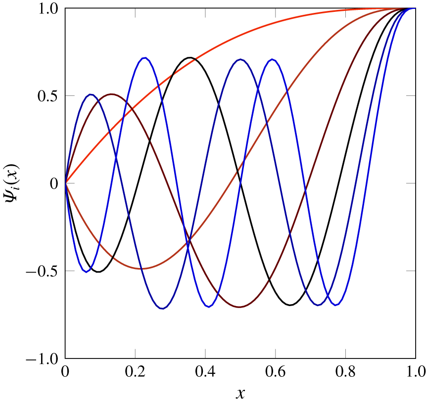
It is noted that direct application of conventional eigenfunctions in the expansion (3.3) hinders the development of the exact evaluation of the non-circulatory velocity potential due to the presence of singular terms. In order to overcome this problem, an expansion of Chebyshev polynomials of the first kind with a sufficiently large number of terms is utilized to approximate each mode shape of the sheet. Polynomial representation of the mode shapes allows the integration in (3.1) to be performed exactly over  $\unicode[STIX]{x1D711}$ with the aid of Glauert’s integral given in (A 1).
Applying the Galerkin technique, equation (3.1) reduces to the well-known second-order form  $\unicode[STIX]{x1D648}\ddot{\boldsymbol{p}}+\unicode[STIX]{x1D63E}\dot{\boldsymbol{p}}+\unicode[STIX]{x1D646}\boldsymbol{p}=\mathbf{0}$ (see (A 7)). Defining the following partitioned vector and matrices of order
 $2M$:
 $$\begin{eqnarray}\unicode[STIX]{x1D667}=\left\{\begin{array}{@{}c@{}}\dot{\unicode[STIX]{x1D665}}\\ \unicode[STIX]{x1D665}\end{array}\right\},\quad \unicode[STIX]{x1D63D}=\left[\begin{array}{@{}cc@{}}\unicode[STIX]{x1D7EC} & \unicode[STIX]{x1D648}\\ \unicode[STIX]{x1D648} & \unicode[STIX]{x1D63E}\end{array}\right],\quad \unicode[STIX]{x1D640}=\left[\begin{array}{@{}cc@{}}-\unicode[STIX]{x1D648} & \unicode[STIX]{x1D7EC}\\ \unicode[STIX]{x1D7EC} & \unicode[STIX]{x1D646}\end{array}\right],\end{eqnarray}$$
the problem reduces into the first-order form  $\unicode[STIX]{x1D63D}\dot{\boldsymbol{r}}+\unicode[STIX]{x1D640}\boldsymbol{r}=\mathbf{0}$. Seeking periodic solutions in the form of
 $\boldsymbol{r}(t)=\tilde{\boldsymbol{r}}\exp (\text{i}\unicode[STIX]{x1D714}t)$, where
 $\tilde{\boldsymbol{r}}$ is the modal amplitude and
 $\unicode[STIX]{x1D714}$ is the complex frequency, one can obtain the following eigenvalue problem
 $[\text{i}\unicode[STIX]{x1D714}\unicode[STIX]{x1D63D}+\unicode[STIX]{x1D640}]\tilde{\boldsymbol{r}}=\mathbf{0}$.
3.2 Numerical results
The dynamics of the linear system is examined by obtaining the eigenfrequencies of the system as a function of the dimensionless flow velocity. The evolution of the generally complex eigenfrequencies of the system with varying flow velocity is commonly displayed as an Argand diagram. In the Argand diagram, the ordinate and the abscissa are associated with the imaginary and real parts of the eigenfrequencies, i.e.  $\text{Im}(\unicode[STIX]{x1D714})$ and
 $\text{Re}(\unicode[STIX]{x1D714})$, respectively. It is recalled that
 $\text{Im}(\unicode[STIX]{x1D714})$ corresponds to the damping ratio, and
 $\text{Re}(\unicode[STIX]{x1D714})$ represents the dimensionless frequency of the oscillation. Instability materializes by the crossing of the eigenfrequency locus from the positive to the negative half-plane in the Argand diagram (i.e. when
 $\text{Im}(\unicode[STIX]{x1D714})<0$); refer to Païdoussis (Reference Païdoussis2014) for more details.
In this study, six modes are employed for numerical solutions (i.e.  $M=6$); this is sufficient for obtaining converged solutions. The other system parameters utilized in the simulations are as follows:
 $L=10~\text{cm}$,
 $h=0.1~\text{mm}$,
 $\unicode[STIX]{x1D70C}=1200~\text{kg}~\text{m}^{-3}$,
 $\unicode[STIX]{x1D70C}_{f}=1.2~\text{kg}~\text{m}^{-3}$,
 $D=2454~\text{N}~\text{cm}^{2}$ and
 $\unicode[STIX]{x1D702}_{s}=0.0002$.
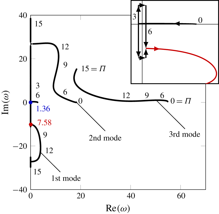
Argand diagram for an inverted flag with  $\unicode[STIX]{x1D707}=1.0$, showing the evolution of the first three modes with the dimensionless flow velocity
 $\unicode[STIX]{x1D6F1}$.

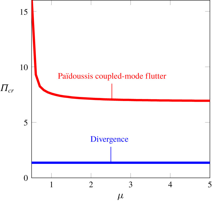
Stability map for a 2-D inverted flag; (——, blue): the onset of divergence, (——, red): the onset of flutter.

Figure 4 is the Argand diagram for an inverted flag with  $\unicode[STIX]{x1D707}=1.0$, showing the evolution of the lowest three eigenfrequencies of the system. The linear response can be interpreted as follows.
(i) Free motion of the inverted flag is damped at low flow velocities; this is evident from the positive imaginary part of the eigenfrequencies.
(ii) At a sufficiently high flow velocity, the frequency of the first mode becomes purely imaginary, and then bifurcates on the
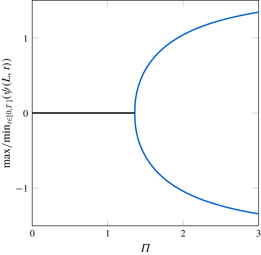
 $\text{Im}(\unicode[STIX]{x1D714})$-axis. One of the solution branches associated with this mode eventually vanishes altogether (i.e. $\text{Re}(\unicode[STIX]{x1D714})=0$, $\text{Im}(\unicode[STIX]{x1D714})=0$) at $\unicode[STIX]{x1D6F1}=1.36$ and crosses from the positive to the negative half-plane, indicating the onset of static divergence (buckling) via a pitchfork bifurcation.
(iii) At a higher flow velocity (
$\unicode[STIX]{x1D6F1}=7.58$), the negative and positive branches of the first mode loci coincide and leave the imaginary axis, while $\text{Im}(\unicode[STIX]{x1D714})<0$ (shown in the inset in this figure). This indicates the onset of Païdoussis-type coupled-mode flutter (Done & Simpson Reference Done and Simpson1977; Païdoussis Reference Païdoussis2014). This bifurcation emanates directly form a divergent state; hence, the frequency of oscillation is zero at the onset of flapping.(iv) The eigenfrequency of the first mode becomes purely imaginary once again as the flow velocity is increased further, at
$\unicode[STIX]{x1D6F1}=14.74$, giving rise to a second buckling of the inverted flag in the first mode.(v) The frequency of the second mode diminishes, and it vanishes circa
$\unicode[STIX]{x1D6F1}=15$.


Let us now consider how well linear theory predicts the dynamics of the system as observed in the experiments. For a physical system, the inverted flag loses its straight, undeformed configuration and buckles similarly to a column under axial load. Thereafter, the flag exhibits flapping motion. Increasing the flow velocity further, the flapping motion gradually diminishes in magnitude, and the flag displays a buckled shape once again, but with a larger amplitude of deformation (compared to the initial buckling) as the fluid dynamic forces grow with increasing flow velocity. Thus, up to this point, the linear model succeeds in predicting, qualitatively at least, the dynamics of the physical system.
It is worth mentioning that stability of the stretched-straight state of the inverted flag up to the occurrence of divergence is not affected by the mass ratio parameter. Thus, for static divergence, the mass ratio does not change the value of the critical flow velocity. This is evident from the stability map shown in figure 5, which highlights the sensitivity of the foregoing bifurcations to the mass ratio parameter. The onset of flapping, however, is sensitive to the mass ratio. More specifically, the Païdoussis-type coupled-mode flutter occurs at considerably higher values of  $\unicode[STIX]{x1D6F1}$ as
 $\unicode[STIX]{x1D707}$ is decreased, in the range
 $\unicode[STIX]{x1D707}\in [0.1\,\,0.6]$. For larger values of
 $\unicode[STIX]{x1D707}$, the change becomes much less significant, and the curve of the boundary of stability displays a near-plateau.
The divergence instability mechanism was originally suggested by the Kim et al. (Reference Kim, Cossé, Huertas Cerdeira and Gharib2013) experiments (where they found that changing the mass ratio does not affect the onset of flapping), and by Sader et al. (Reference Sader, Cossé, Kim, Fan and Gharib2016a) theoretically via a linear stability analysis. Sader et al. (Reference Sader, Cossé, Kim, Fan and Gharib2016a) argued that the divergence instability of the inverted flag is a steady process, with steady aerodynamic forces being involved. Then, unsteadiness in the flow comes into play and leads to flapping motion. This is also predicted by the nonlinear model in the next section.
Before closing this section, an important note should be made. Since linear theory is valid only up to the onset of the first instability, in this case divergence, the system must be analysed by the nonlinear model to ascertain the reliability of the predicted post-divergence behaviour. Thus, the loss of the stability of the original equilibrium predicted by the linear model is valid. However, other states may be encountered once nonlinear effects are taken into account. The reason for this is that, in the linear model, it is assumed that motions are small, remaining in the proximity of the undeflected equilibrium. This is not the case for larger values of the flow velocity, where the inverted flag diverges considerably, away from original equilibrium.
4 Post-divergence behaviour
The nonlinear aspects of the system dynamics, such as limit-cycle frequencies and amplitudes, as well as the transition between the various dynamical states, are studied numerically. The nonlinear integro-partial-differential model of (2.24) is first discretized in space, and then recast in a system of first-order ODEs. The resultant set of ODEs is solved using a pseudo-arclength continuation technique. The Gear backward differentiation formula is also used to obtain the time histories of oscillation.
4.1 Nonlinear discretized model
The spatial discretization of the nonlinear equation of motion (2.24) is made in a similar fashion to that described in § 3.1 by employing the Galerkin method. Hence, a linear combination of suitable comparison functions  $\unicode[STIX]{x1D6F9}_{i}(x)$ is selected to approximate the rotation of the flag
 $$\begin{eqnarray}\unicode[STIX]{x1D713}(x,t)=\mathop{\sum }_{i=1}^{M}\unicode[STIX]{x1D6F9}_{i}(x)q_{i}(t),\end{eqnarray}$$
where  $q_{i}(t)$ represent the unknown time-dependent generalized coordinates;
 $M$ denotes the number of modes used.
As discussed in § 3.1, Chebyshev polynomials of the first kind with a sufficient number of terms are utilized to approximate the comparison functions  $\unicode[STIX]{x1D6F9}_{i}(x)$ (see (A 8)). Applying Galerkin’s technique, i.e. inserting (4.1) into (2.24), multiplying it by the corresponding comparison functions and integrating the resulting equation with respect to the spatial coordinate from
 $0$ to
 $1$ results in a set of
 $M$ second-order ODEs with trigonometric nonlinearities
 $$\begin{eqnarray}\displaystyle & & \displaystyle \unicode[STIX]{x1D6FD}\mathop{\sum }_{j=1}^{M}\left(\int _{0}^{1}\unicode[STIX]{x1D6F9}_{i}\unicode[STIX]{x1D6F9}_{j}\,\text{d}x\right)\ddot{q}_{j}-\unicode[STIX]{x1D702}_{s}\mathop{\sum }_{j=1}^{M}\left(\int _{0}^{1}\unicode[STIX]{x1D6F9}_{i}\unicode[STIX]{x1D6F9}_{j}^{\prime \prime }\,\text{d}x\right)\dot{q}_{j}-\mathop{\sum }_{j=1}^{M}\left(\int _{0}^{1}\unicode[STIX]{x1D6F9}_{i}\unicode[STIX]{x1D6F9}_{j}^{\prime \prime }\,\text{d}x\right)q_{j}\nonumber\\ \displaystyle & & \displaystyle \quad +\,\int _{0}^{1}\unicode[STIX]{x1D6F9}_{i}(x)\left[\sin \left(\mathop{\sum }_{j=1}^{M}\unicode[STIX]{x1D6F9}_{j}(x)q_{j}(t)\right)\right.\nonumber\\ \displaystyle & & \displaystyle \quad \times \left.\int _{1}^{x}\int _{0}^{s}\unicode[STIX]{x2202}_{tt}\left(\mathop{\sum }_{j=1}^{M}\unicode[STIX]{x1D6F9}_{j}(\unicode[STIX]{x1D709})q_{j}(t)\right)\sin \left(\mathop{\sum }_{j=1}^{M}\unicode[STIX]{x1D6F9}_{j}(\unicode[STIX]{x1D709})q_{j}(t)\right)\,\text{d}\unicode[STIX]{x1D709}\,\text{d}s\right]\,\text{d}x\nonumber\\ \displaystyle & & \displaystyle \quad +\,\int _{0}^{1}\unicode[STIX]{x1D6F9}_{i}(x)\left[\cos \left(\mathop{\sum }_{j=1}^{M}\unicode[STIX]{x1D6F9}_{j}(x)q_{j}(t)\right)\right.\nonumber\\ \displaystyle & & \displaystyle \quad \times \left.\int _{1}^{x}\int _{0}^{s}\unicode[STIX]{x2202}_{tt}\left(\mathop{\sum }_{j=1}^{M}\unicode[STIX]{x1D6F9}_{j}(\unicode[STIX]{x1D709})q_{j}(t)\right)\cos \left(\mathop{\sum }_{j=1}^{M}\unicode[STIX]{x1D6F9}_{j}(\unicode[STIX]{x1D709})q_{j}(t)\right)\,\text{d}\unicode[STIX]{x1D709}\,\text{d}s\right]\,\text{d}x\nonumber\\ \displaystyle & & \displaystyle \quad +\,\int _{0}^{1}\unicode[STIX]{x1D6F9}_{i}(x)\left[\sin \left(\mathop{\sum }_{j=1}^{M}\unicode[STIX]{x1D6F9}_{j}(x)q_{j}(t)\right)\right.\nonumber\\ \displaystyle & & \displaystyle \quad \times \left.\int _{1}^{x}\int _{0}^{s}\left(\unicode[STIX]{x2202}_{t}\left(\mathop{\sum }_{j=1}^{M}\unicode[STIX]{x1D6F9}_{j}(\unicode[STIX]{x1D709})q_{j}(t)\right)\right)^{2}\cos \left(\mathop{\sum }_{j=1}^{M}\unicode[STIX]{x1D6F9}_{j}(\unicode[STIX]{x1D709})q_{j}(t)\right)\,\text{d}\unicode[STIX]{x1D709}\,\text{d}s\right]\,\text{d}x\nonumber\\ \displaystyle & & \displaystyle \quad -\,\int _{0}^{1}\unicode[STIX]{x1D6F9}_{i}(x)\left[\cos \left(\mathop{\sum }_{j=1}^{M}\unicode[STIX]{x1D6F9}_{j}(x)q_{j}(t)\right)\right.\nonumber\\ \displaystyle & & \displaystyle \quad \times \left.\int _{1}^{x}\int _{0}^{s}\left(\unicode[STIX]{x2202}_{t}\left(\mathop{\sum }_{j=1}^{M}\unicode[STIX]{x1D6F9}_{j}(\unicode[STIX]{x1D709})q_{j}(t)\right)\right)^{2}\sin \left(\mathop{\sum }_{j=1}^{M}\unicode[STIX]{x1D6F9}_{j}(\unicode[STIX]{x1D709})q_{j}(t)\right)\,\text{d}\unicode[STIX]{x1D709}\,\text{d}s\right]\,\text{d}x\nonumber\\ \displaystyle & & \displaystyle \quad +\,\int _{0}^{1}\unicode[STIX]{x1D6F9}_{i}(x)\left[\cos \left(\mathop{\sum }_{j=1}^{M}\unicode[STIX]{x1D6F9}_{j}(x)q_{j}(t)\right)\int _{1}^{x}\unicode[STIX]{x0394}p(s,t)\cos \left(\mathop{\sum }_{j=1}^{M}\unicode[STIX]{x1D6F9}_{j}(x)q_{j}(t)\right)\,\text{d}s\right]\,\text{d}x\nonumber\\ \displaystyle & & \displaystyle \quad +\,\int _{0}^{1}\unicode[STIX]{x1D6F9}_{i}(x)\left[\sin \left(\mathop{\sum }_{j=1}^{M}\unicode[STIX]{x1D6F9}_{j}(x)q_{j}(t)\right)\int _{1}^{x}\unicode[STIX]{x0394}p(s,t)\sin \left(\mathop{\sum }_{j=1}^{M}\unicode[STIX]{x1D6F9}_{j}(x)q_{j}(t)\right)\,\text{d}s\right]\,\text{d}x\nonumber\\ \displaystyle & & \displaystyle \quad -\,\left(f_{p}(t)\sin \left(\mathop{\sum }_{j=1}^{M}\unicode[STIX]{x1D6F9}_{j}(1)q_{j}(t)\right)\right)\int _{0}^{1}\unicode[STIX]{x1D6F9}_{i}(x)\sin \left(\mathop{\sum }_{j=1}^{M}\unicode[STIX]{x1D6F9}_{j}(x)q_{j}(t)\right)\,\text{d}x\nonumber\\ \displaystyle & & \displaystyle \quad -\,\left(f_{p}(t)\cos \left(\mathop{\sum }_{j=1}^{M}\unicode[STIX]{x1D6F9}_{j}(1)q_{j}(t)\right)\right)\int _{0}^{1}\unicode[STIX]{x1D6F9}_{i}(x)\cos \left(\mathop{\sum }_{j=1}^{M}\unicode[STIX]{x1D6F9}_{j}(x)q_{j}(t)\right)\,\text{d}x=0,\end{eqnarray}$$
with  $\unicode[STIX]{x0394}p$ and
 $f_{p}$ denoting the dimensionless counterparts of
 $\unicode[STIX]{x0394}P$ and
 $F_{p}$, respectively; the prime denotes a spatial derivative.
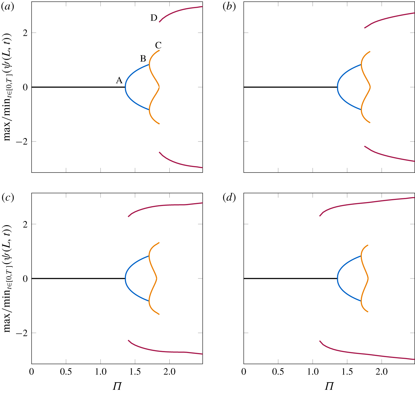
It is evident from (4.2) that sine and cosine terms have been retained intact in the discretization scheme and the numerical integration. Consequently, the number of terms in the discretized system and, in turn, the computational cost, increase significantly. Nevertheless, this ensures that reliable predictions are made when the flag deformation becomes very large, at high flow velocities (Tavallaeinejad et al. Reference Tavallaeinejad, Païdoussis and Legrand2018). In this study, six generalized coordinates are retained in the series expansion of the rotation angle, resulting in  $6$ second-order ODEs. These equations are then recast into state-space form, i.e. a set of twelve first-order ODEs, and are solved using the pseudo-arclength continuation technique implemented in AUTO (Doedel et al. Reference Doedel, Champneys, Fairgrieve, Kuznetsov, Sandstede and Wang1997) to construct the bifurcation diagrams. This technique enables us to perform continuation of both stable and unstable branches of the solution. Direct time integration is also performed via Gear’s backward differentiation formula (Gear Reference Gear1971) yielding the time-varying generalized coordinates
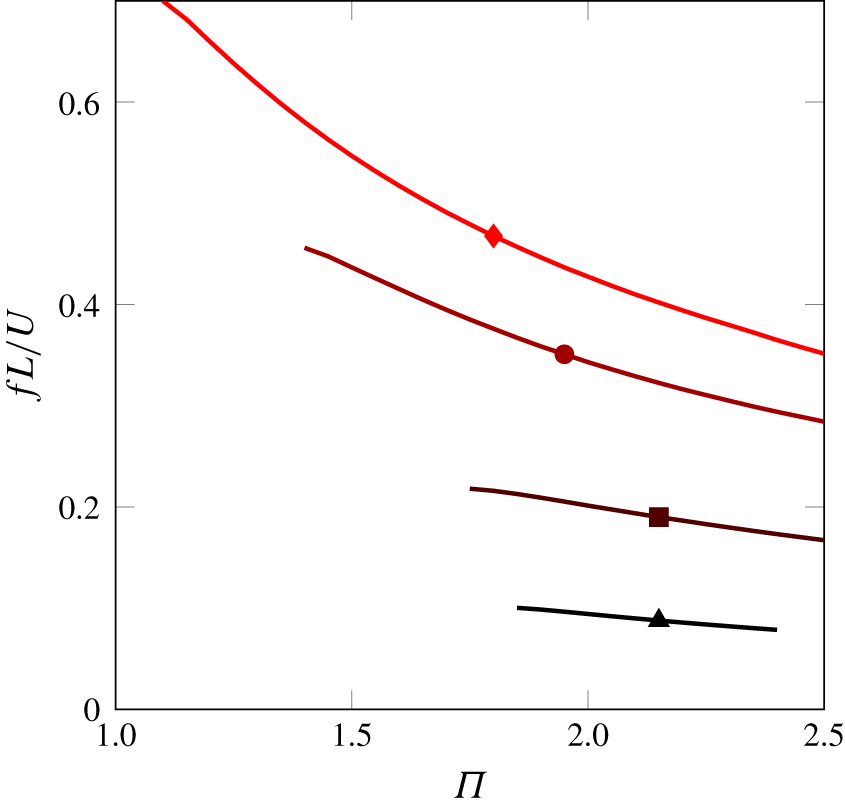
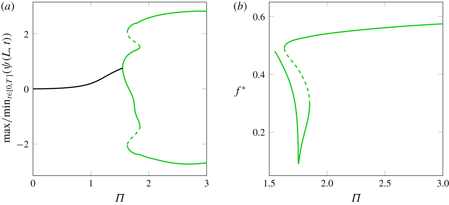
 $q_{i}$. Time histories of the amplitude of oscillation are used to plot phase-plane portraits, Fast Fourier transforms (FFT), and (flapping) flag shapes at points of interest in the parameter space. In some cases, where the change in the state of the system is sharp, the stable periodic solution emerging from a saddle-node bifurcation is numerically traced via direct time integration, using the calculated generalized coordinates at a given flow velocity as initial conditions for the next flow velocity. In order to plot the flag shapes in various states, the transverse and longitudinal motions (i.e.
 $w(x,t)$ and
 $u(x,t)$, respectively) are retrieved, making use of the integral form of (2.2).
4.2 Numerical results
The numerical results from the nonlinear model are shown in the form of bifurcation diagrams, in which the ordinate is the maximum tip rotation of the inverted flag and the abscissa is the dimensionless flow velocity  $\unicode[STIX]{x1D6F1}$. The system parameters in § 3.2 are again utilized in this section. The convention in all bifurcation diagrams is as follows: continuous and dashed lines represent stable and unstable branches of the solution, respectively. A stable solution represents either a buckled state corresponding to static equilibrium, or the amplitude of oscillation for flapping. Each colour used in the bifurcation diagrams corresponds to a specific regime of dynamical behaviour in the considered range of flow velocities.
Bifurcation diagram for a two-dimensional inverted flag with  $\unicode[STIX]{x1D707}=1.0$, indicating the minimum and maximum values of the leading-edge rotation over a cycle of steady-state oscillation of period
 $T^{\ast }$. (——, black) Undeflected stable equilibrium; (——, blue) deflected stable equilibrium corresponding to buckling of the inverted flag to either side; (——, orange) stable periodic solutions (oscillation around deflected equilibria) corresponding to deformed flapping of the inverted flag to either side; (——, brown) stable periodic solution (oscillations around undeflected equilibrium). This colour scheme is also utilized in figures 7–10.

Figure 6 gives the bifurcation diagram for a two-dimensional inverted flag with  $\unicode[STIX]{x1D707}=1.0$, demonstrating four distinct states/regimes, which can be summarized as follows.
(i) Stretched-straight state: as also expected from the linear analysis, the trivial solution associated with the undeflected static equilibrium is stable at small flow velocities. Small perturbations generate motions which ultimately die out, and the inverted flag remains stable at its undeflected equilibrium, as illustrated in figure 7(a). This regime was first identified by Kim et al. (Reference Kim, Cossé, Huertas Cerdeira and Gharib2013) and its stability was characterized to some extent by Kim et al. (Reference Kim, Cossé, Huertas Cerdeira and Gharib2013), Gurugubelli & Jaiman (Reference Gurugubelli and Jaiman2015) and Sader et al. (Reference Sader, Cossé, Kim, Fan and Gharib2016a).
(ii) Buckled state: the undeflected static equilibrium loses stability at point A where
$\unicode[STIX]{x1D6F1}=1.36$ through a supercritical pitchfork bifurcation, in line with the linear model. This leads to divergence (buckling) in the first mode, the amplitude of which increases with flow velocity (see figure 7(b)). The existence of the buckled state was first reported by Gurugubelli & Jaiman (Reference Gurugubelli and Jaiman2015), observed experimentally by Yu et al. (Reference Yu, Liu and Chen2017) and subsequently demonstrated to be an equilibrium of the inverted flag system by Goza et al. (Reference Goza, Colonius and Sader2018).(iii) Deformed-flapping state: the deflected solution loses stability via a supercritical Hopf bifurcation at point B where
$\unicode[STIX]{x1D6F1}=1.70$, leading to ‘deformed-flapping motions’, that is periodic oscillation around the buckled state. The response is predominantly in the first mode of a cantilevered beam. This motion lasts over the range of $\unicode[STIX]{x1D6F1}\in [1.70\,\,1.82]$, and the amplitude of oscillation increases with $\unicode[STIX]{x1D6F1}$, as illustrated in figure 7(c,d). Additional features of the system dynamics are given in figure 8, displaying the time history, phase-plane portrait and FFT plot at $\unicode[STIX]{x1D6F1}=1.80$, all indicating a periodic motion; the dimensionless frequency of oscillation is $f^{\ast }=0.33$. The appearance of deformed flapping was identified by Yu et al. (Reference Yu, Liu and Chen2017), and its emergence was reported to be via a supercritical Hopf bifurcation by Goza et al. (Reference Goza, Colonius and Sader2018).(iv) Large-amplitude flapping state: increasing the flow velocity further causes a transition from the deformed-flapping regime to flapping around the undeflected equilibrium, the amplitude of which increases with the flow velocity. The transition is accompanied by a jump in the amplitude of flapping via two saddle-node bifurcations at points C and D, at
$\unicode[STIX]{x1D6F1}=1.82$ and $\unicode[STIX]{x1D6F1}=1.65$, respectively. This forms a region wherein the response of the system is attracted by either the stable limit cycle around the deflected equilibrium or that around the undeflected equilibrium. Hence, the behaviour of the system is indeed subcritical. The existence of this bistable zone implies the existence of an unstable repelling limit cycle (not shown in the bifurcation diagram as AUTO was unable to find it) bounded by the two saddle-node bifurcations. Figure 9 shows the time history, phase-plane portrait and FFT plot for $\unicode[STIX]{x1D6F1}=1.65$, all displaying a periodic motion; the dimensionless frequency of oscillation is $f^{\ast }=0.52$. This regime has been characterized in a number of references (see, for instance, Gurugubelli & Jaiman (Reference Gurugubelli and Jaiman2015), Shoele & Mittal (Reference Shoele and Mittal2016a) and Goza et al. (Reference Goza, Colonius and Sader2018)).


Shapes of the two-dimensional inverted flag studied in figure 6: (a) stretched-straight state ( $\unicode[STIX]{x1D6F1}=1.35$), (b) buckled state (
 $\unicode[STIX]{x1D6F1}=1.40$), (c) at the onset of deformed-flapping mode (
 $\unicode[STIX]{x1D6F1}=1.71$), (d) deformed-flapping mode (
 $\unicode[STIX]{x1D6F1}=1.75$) and (e) large-amplitude flapping (
 $\unicode[STIX]{x1D6F1}=1.65$). Colour scheme as in figure 6.

Response of the inverted flag, with  $\unicode[STIX]{x1D707}=1.0$ at
 $\unicode[STIX]{x1D6F1}=1.80$, displaying a periodic motion around the deflected equilibrium; (a) time history, (b) phase portrait and (c) the frequency content of the response, obtained from FFT. Colour scheme as in figure 6.

Response of the inverted flag with  $\unicode[STIX]{x1D707}=1.0$ at
 $\unicode[STIX]{x1D6F1}=1.65$, displaying a periodic motion around the undeflected equilibrium; (a) time history, (b) phase-plane portrait and (c) the frequency content of the response, obtained from FFT. Colour scheme as in figure 6.

The qualitative dynamical behaviour of the inverted flag with increasing flow velocity is illustrated in figure 7, showing successively the stretched-straight, buckled, deformed-flapping and the large-amplitude flapping states.
Figure 10 shows the sensitivity of  $f^{\ast }$ to the dimensionless flow velocity
 $\unicode[STIX]{x1D6F1}$. As depicted,
 $f^{\ast }$ sharply decreases with increasing
 $\unicode[STIX]{x1D6F1}$ in the deformed-flapping regime, while it increases only slightly in the large-amplitude flapping regime as
 $\unicode[STIX]{x1D6F1}$ is increased. This latter aspect is in good agreement with the experimental measurements by Sader et al. (Reference Sader, Cossé, Kim, Fan and Gharib2016a), which confirms that the large-amplitude flapping frequency varies only slightly with flow velocity.
Dimensionless frequency  $f^{\ast }$ versus dimensionless flow velocity
 $\unicode[STIX]{x1D6F1}$ for an inverted flag with
 $\unicode[STIX]{x1D707}=1.0$. Colour scheme as in figure 6.

The model developed in the present study is believed to simulate fairly accurately the effect of fluid flow on stability of the system, since it is capable of predicting reasonably well the dynamical response of the system up to moderate angles of attack. It is nevertheless realized that the flag exhibits highly curved shapes in the course of large-amplitude flapping (see figure 7), signalling that the limit of applicability of inviscid flow theory may well have been surpassed.
At very large angles of attack, massive separation occurs at the leading edge of the flag, resulting in a sharp drop in the normal force, which in turn causes a sudden oscillation decrease. This phenomenon is not captured by inviscid flow theory which, in principle, cannot model such viscous effects. Interestingly, nevertheless, the ‘qualitative route’ (i.e. stability, buckling, deformed flapping and large-amplitude flapping), as well as the bifurcation values for  $\unicode[STIX]{x1D6F1}$ are in very good agreement with the fully coupled computational study of Goza et al. (Reference Goza, Colonius and Sader2018), who conducted simulations using an immersed boundary method. For example, for a two-dimensional inverted flag with
 $\unicode[STIX]{x1D707}=0.2$ (which is the reciprocal of the dimensionless mass ratio used by Goza et al. (Reference Goza, Colonius and Sader2018), denoted by
 $M_{\unicode[STIX]{x1D70C}}=5.0$), the present model predicts the onset of divergence (pitchfork bifurcation) at
 $\unicode[STIX]{x1D6F1}_{A}=1.36$, the onset of deformed flapping (Hopf bifurcation) at
 $\unicode[STIX]{x1D6F1}_{B}=1.71$ and the onset of large-amplitude flapping (saddle-node bifurcation) at
 $\unicode[STIX]{x1D6F1}_{D}=1.80$, while the computational model of Goza et al. (Reference Goza, Colonius and Sader2018) predicts
 $\unicode[STIX]{x1D6F1}_{A}=1.42$,
 $\unicode[STIX]{x1D6F1}_{B}=1.55$ and
 $\unicode[STIX]{x1D6F1}_{D}=1.78$, respectively. A more complete comparison between the results of the present model and those of Goza et al. (Reference Goza, Colonius and Sader2018) is provided in § 5. It should be noted that the simulations by Goza et al. (Reference Goza, Colonius and Sader2018) were performed in the
 $Re=200$ flow regime, while the results obtained via the present model correspond to a higher flow regime,
 $Re\sim O(10^{5})$.
An additional comment is useful here. The buckled and deformed-flapping regimes predicted by the proposed model and the simulations of Goza et al. (Reference Goza, Colonius and Sader2018) have not been observed in the experiments of Kim et al. (Reference Kim, Cossé, Huertas Cerdeira and Gharib2013). Nevertheless, these two regimes are experimentally identified in the measurements of Yu et al. (Reference Yu, Liu and Chen2017). It is noted that Yu et al. (Reference Yu, Liu and Chen2017) used a channel with a half-width dimension equal to the flag length (and hence, close to the flapping amplitude). Thus, the flow was partially blocked, which may have affected the dynamics. Additionally, the existence of the (unstable) deflected equilibrium was observed experimentally by Sader et al. (Reference Sader, Huertas-Cerdeira and Gharib2016b) via the introduction of additional damping.
The numerical results in figure 6 offer a plausible explanation for the above-mentioned discrepancy. It is known that there is a potential for hysteresis in the onset of flapping, resulting in a bistable region. For a physical flag, the existence of this phenomenon gives rise to the possibility of a sudden jump from quiescent undeflected equilibrium to large-amplitude flapping motion, without encountering other states. Vortex shedding, overshoots during flow-speed increments, or incoming flow turbulence may provide a sufficiently strong disturbance for the jump to occur.
The absence of unsteady vortex shedding in the model proposed in this paper could well explain the discrepancy in the predicted sequence of displayed regimes and experimental observations. However, it should be noted that in the low- $Re$ simulations by Goza et al. (Reference Goza, Colonius and Sader2018) and Ryu et al. (Reference Ryu, Park, Kim and Sung2015) (
 $Re=200$), as well as high-
 $Re$ simulations by Gurugubelli & Jaiman (Reference Gurugubelli and Jaiman2019) (
 $Re=30\,000$), vortex shedding is present, yet the deformed-flapping regime is observed in these studies over a range of flow speeds, in contrast to experimental observations of Kim et al. (Reference Kim, Cossé, Huertas Cerdeira and Gharib2013). Indeed, the relationship between experimentally observed regime transitions and the predictions of low- and high-
 $Re$ simulations is an interesting avenue for further experimental and theoretical research.
The numerical results discussed here suggest that ‘fluidelastic instabilities’ may be the underlying mechanisms for the rich dynamical behaviour displayed by two-dimensional, strictly speaking heavy inverted flags. Thus, the flapping motion may be viewed as a ‘self-excited oscillation’, that is flutter. The same mechanism is responsible for flapping of conventional flags in axial flow. More specifically, the proposed model is developed based on self-excited (or movement-induced) vibration principles and does not include flow instability and its consequences, such as vortex-shedding-induced fluctuating loads. Nevertheless, it does capture qualitatively the bifurcations, as well as some detailed intricate dynamics (including the large-amplitude flapping regime), observed in previous studies for small mass ratio flags.
4.3 Influence of mass ratio
As discussed in the foregoing, the undeflected equilibrium of the inverted flag loses stability first via divergence, and the post-buckling response of the system remains static prior to the occurrence of a Hopf bifurcation. As seen from (2.24), the mass ratio parameter  $\unicode[STIX]{x1D707}$ is present only in the time-dependent terms. Thus, it is expected that
 $\unicode[STIX]{x1D707}$ has no impact on the critical point for divergence or the existence of the deflected equilibria. This conclusion agrees well with experimental/theoretical findings of Sader et al. (Reference Sader, Cossé, Kim, Fan and Gharib2016a) for the onset of divergence. The existence of a deflected equilibrium following the onset of divergence was realized in their experiments by introducing additional damping by touching the flag with a slender rigid pole.
The mass ratio  $\unicode[STIX]{x1D707}$, on the other hand, does affect the dynamical behaviour of the system and significantly affects the stability of the associated solution branches. Setting the time-dependent fluid forces to zero (all terms multiplied by
 $\unicode[STIX]{x1D707}$ in (2.24) disappear) results in governing equations equivalent to a model for an inverted flag subject only to steady-flow forces. As can be seen from figure 11, the deflected static solutions branching off from the pitchfork bifurcation point remain stable with increasing flow velocity. On the other hand, considering all time-dependent fluid forces (with
 $\unicode[STIX]{x1D707}\neq 0$) and performing a stability analysis leads to the detection of Hopf bifurcations on each deflected static solution, giving rise to periodic solutions, i.e. flutter.
Bifurcation diagram of an inverted flag subjected to steady fluid forces showing the leading-edge rotation angle versus dimensionless flow velocity. (——, black) Undeflected stable equilibrium and (——, blue) deflected static equilibrium solutions corresponding to buckling of the inverted flag to either side. No secondary bifurcation (dynamic or static) materializes. Colour scheme as in figure 6.

Figure 12 shows how  $\unicode[STIX]{x1D707}$ affects the nonlinear response of the system. It is seen that the stability of the trivial solution, the critical flow velocities for divergence and (virtually) the Hopf bifurcation are not affected by
 $\unicode[STIX]{x1D707}$. The post-critical behaviour, on the other hand, is significantly altered. For instance, for
 $\unicode[STIX]{x1D707}=0.5$, the critical values of the flow velocity are
 $\unicode[STIX]{x1D6F1}_{A}=1.36$,
 $\unicode[STIX]{x1D6F1}_{B}=1.70$,
 $\unicode[STIX]{x1D6F1}_{C}=1.83$ and
 $\unicode[STIX]{x1D6F1}_{D}=1.75$, while for
 $\unicode[STIX]{x1D707}=5.0$ these values are
 $\unicode[STIX]{x1D6F1}_{A}=1.36$,
 $\unicode[STIX]{x1D6F1}_{B}=1.70$,
 $\unicode[STIX]{x1D6F1}_{C}=1.80$ and
 $\unicode[STIX]{x1D6F1}_{D}=1.40$.
Bifurcation diagrams for a two-dimensional inverted flag with different mass ratios: (a)  $\unicode[STIX]{x1D707}=0.1$, (b)
 $\unicode[STIX]{x1D707}=0.5$, (c)
 $\unicode[STIX]{x1D707}=2.0$ and (d)
 $\unicode[STIX]{x1D707}=5.0$, indicating the minimum and maximum values of the leading-edge rotation over a cycle of steady-state oscillation of period
 $T^{\ast }$. (——, black) Stable static solution (undeflected stable equilibria); (——, blue) stable static solutions (deflected static equilibria) corresponding to buckling of the inverted flag to either side; (——, orange) stable periodic solutions (oscillation around deflected equilibria) corresponding to deformed flapping of the inverted flag to either side; (——, brown) stable periodic solutions (oscillations around undeflected equilibrium). Colour scheme as in figure 6.

Two additional points should be made here about the effects of the mass ratio parameter on the dynamics of the system. First, the critical flow velocity for the Hopf bifurcation,  $\unicode[STIX]{x1D6F1}_{B}$, obtained via the nonlinear model, is considerably lower than that obtained via the linearized model. This may be explained by considering the fact that a linear model assumes that instability emanates from the position of rest where the deflections are vanishingly small. However, in reality, once a divergence has developed, deflections away from the equilibrium state develop and grow with increasing flow velocity. As the deflection becomes larger, the nonlinear fluid-related forces become stronger. This causes a Hopf bifurcation, leading to a limit-cycle oscillation, to occur at appreciably different, and in this case lower, flow velocities, compared to the predictions of the linear model.
Secondly, as seen from figure 12, for sufficiently large  $\unicode[STIX]{x1D707}$ (i.e. for a light flag or a heavily loaded flag), the transition to large-amplitude flapping becomes strongly subcritical. An unstable periodic solution (not shown here as AUTO was unable to find it) which originates form the periodic solution around the deflected equilibrium (i.e. at
 $\unicode[STIX]{x1D6F1}_{C}$) goes backward and folds at a flow velocity (i.e.
 $\unicode[STIX]{x1D6F1}_{D}$) even lower than that for the onset of divergence. Refer to figure 6 for definitions of
 $\unicode[STIX]{x1D6F1}_{C}$ and
 $\unicode[STIX]{x1D6F1}_{D}$. The unstable solution then becomes stable, generating the large-amplitude periodic solution. The existence of this solution would give rise to the possibility of a sudden jump from static undeflected equilibrium to large-amplitude flapping motion, without encountering other states. More specifically, considering the case of
 $\unicode[STIX]{x1D707}=5.0$ (figure 12d), two stable solutions coexist for
 $\unicode[STIX]{x1D6F1}\in [1.10\,\,1.36]$: the trivial solution and a large-amplitude periodic one. For
 $\unicode[STIX]{x1D6F1}=1.20$, for instance, small perturbations about the undeflected equilibrium would die out and the inverted flag would come to rest at the original static equilibrium. Perturbations of sufficiently large amplitude, on the other hand, could lead the system to enter into the large-amplitude flapping state, without experiencing the usual route outlined in § 4.2. Interestingly, the results in figure 12 highlight that light flags are more likely to exhibit hysteresis in the onset of large-amplitude flapping.
Figure 13 shows the variation of the reduced frequency as a function of the dimensionless flow velocity for different values of mass ratio. Here, to be able to compare the numerical values for flapping frequency with those obtained by Goza et al. (Reference Goza, Colonius and Sader2018) and Shoele & Mittal (Reference Shoele and Mittal2016a), a fluid time scale, defined as  $\unicode[STIX]{x1D70F}_{f}=L/U$, is used to non-dimensionalize the flapping frequency
 $f$. Thus, the reduced frequency is defined as
 $f_{R}=fL/U=f^{\ast }\sqrt{\unicode[STIX]{x1D707}}/\unicode[STIX]{x1D6F1}$. The notation adopted here can be linked to that used in § 2.3.2 as
 $f_{R}=k/\unicode[STIX]{x03C0}$. As seen in the figure, for all cases studied,
 $f_{R}$ decreases monotonically with increasing
 $\unicode[STIX]{x1D6F1}$. For heavier flags (and thus lower mass ratios), the reduced frequency decreases approximately linearly with
 $\unicode[STIX]{x1D6F1}$.
As also seen in figure 13, the reduced frequency decreases as  $\unicode[STIX]{x1D707}$ is decreased. For example, for the heaviest flag with
 $\unicode[STIX]{x1D707}=0.1$, the reduced frequency is
 $f_{R}=0.09$ at
 $\unicode[STIX]{x1D6F1}=2.0$, while for the lightest flag with
 $\unicode[STIX]{x1D707}=5.0$,
 $f_{R}=0.43$. The reduction of flapping frequency with mass ratio is in line with Gurugubelli & Jaiman’s predictions. Strikingly, the results in figure 13 indicate that the dimensionless flapping frequency lies in the range
 $0.1\lesssim f_{R}\lesssim 0.2$, for
 $\unicode[STIX]{x1D707}=0.3$, which agrees well with predictions by Shoele & Mittal (Reference Shoele and Mittal2016a) and Goza et al. (Reference Goza, Colonius and Sader2018), and measurements by Kim et al. (Reference Kim, Cossé, Huertas Cerdeira and Gharib2013). This suggests that the absence of unsteady vortex shedding in the model may have a minimal impact on the dynamical behaviour of heavy flags. For lighter flags (or heavier fluid forcing), on the other hand, the model overestimates the flapping frequency as compared to the measurements of Yu et al. (Reference Yu, Liu and Chen2017) who reported that the dimensionless flapping frequency reaches to
 $f_{R}=0.18$, with the shedding frequency of the vortices being twice the flapping frequency of the inverted flag. Thus, the unsteady vortex shedding could well be central for light flags by virtue of injecting another time scale into the problem, and therefore may not be ignored.
The reduced frequency may be considered as a measure of the unsteadiness of the flow. It is generally acceptable to use quasi-steady-flow theory for a body oscillating with a low value of reduced frequency in fluid flow (Hodges & Pierce Reference Hodges and Pierce2011). Small values of the reduced frequency allow sufficient time for vortex formation and shedding from the trailing edge (Shoele & Mittal Reference Shoele and Mittal2016a). Thus, the results shown in figure 13 suggest that the quasi-steady flow theory may be more appropriate for predicting the dynamics of heavier flags.
Sensitivity of the large-amplitude flapping reduced frequency to the dimensionless flow velocity  $\unicode[STIX]{x1D6F1}$ for inverted flags of different mass ratios: (▴)
 $\unicode[STIX]{x1D707}=0.1$; (▪)
 $\unicode[STIX]{x1D707}=0.5$; (●)
 $\unicode[STIX]{x1D707}=2.0$; and (♦)
 $\unicode[STIX]{x1D707}=5.0$.

4.4 Influence of angle of attack
It is of interest to explore the dynamical behaviour of inverted flags when they are subject to oncoming flow with a non-zero angle of attack  $\unicode[STIX]{x1D713}_{0}$, as illustrated in figure 14. Note that
 $\unicode[STIX]{x1D713}_{0}$ is constant with respect to temporal and spatial coordinates.
The projection of the undisturbed flow velocity onto the  $X$ and
 $Z$ directions leads to
 $U_{X}=\boldsymbol{U}\boldsymbol{\cdot }\boldsymbol{e}_{X}=U\cos \unicode[STIX]{x1D713}_{0}$ and
 $U_{Z}=\boldsymbol{U}\boldsymbol{\cdot }\boldsymbol{e}_{Z}=U\sin \unicode[STIX]{x1D713}_{0}$, respectively. Consequently, the normal and tangential components of the relative flow velocity in (2.3), and in turn the fluid-related forces, should be revised in order to take into account both components. Hence,
 $$\begin{eqnarray}\displaystyle & \displaystyle V_{n}(x,t)=({\dot{w}}-U\sin \unicode[STIX]{x1D713}_{0})\cos \unicode[STIX]{x1D713}-(\dot{u}+U\cos \unicode[STIX]{x1D713}_{0})\sin \unicode[STIX]{x1D713}, & \displaystyle\end{eqnarray}$$
 $$\begin{eqnarray}\displaystyle & \displaystyle V_{\unicode[STIX]{x1D70F}}(x,t)=(\dot{u}+U\cos \unicode[STIX]{x1D713}_{0})\cos \unicode[STIX]{x1D713}+({\dot{w}}-U\sin \unicode[STIX]{x1D713}_{0})\sin \unicode[STIX]{x1D713}. & \displaystyle\end{eqnarray}$$
Inverted flag in axial flow with a small initial angle of attack  $\unicode[STIX]{x1D713}_{0}$.

Nonlinear response of a two-dimensional inverted flag with  $\unicode[STIX]{x1D707}=1.0$ and
 $\unicode[STIX]{x1D713}_{0}=0.1$. (a) Bifurcation diagram indicating the minimum and maximum values of the leading-edge rotation over a cycle of steady-state oscillation of period
 $T^{\ast }$: (——, black) stable static solution; (– – –) unstable and (——, green) stable periodic solution (asymmetric oscillations). (b) Dimensionless frequency
 $f^{\ast }$ versus dimensionless flow velocity
 $\unicode[STIX]{x1D6F1}$.

Bifurcation diagrams for  $\unicode[STIX]{x1D713}_{0}=0.2$ and various mass ratios: (a)
 $\unicode[STIX]{x1D707}=0.1$, (b)
 $\unicode[STIX]{x1D707}=0.5$, (c)
 $\unicode[STIX]{x1D707}=2.0$ and (d)
 $\unicode[STIX]{x1D707}=5.0$, indicating the minimum and maximum values of the leading-edge rotation over a cycle of steady-state oscillation of period
 $T^{\ast }$. (——, black) Stable static solution; (– – –) unstable and (——, green) stable periodic solutions (asymmetric oscillations).

The bifurcation diagram and the flapping frequency for a 2-D inverted flag with  $\unicode[STIX]{x1D707}=1.0$, and
 $\unicode[STIX]{x1D713}_{0}=0.1\approx 5.7^{\circ }$ are plotted in figure 15. Even such a seemingly small angle of attack gives rise to asymmetric fluid loading on the inverted flag, which consequently breaks the symmetry of the nonlinear response. More specifically, the supercritical pitchfork bifurcation ‘point’ (point A in figure 6) is replaced by a gradual transition from small to large deflections. In contrast to the case of
 $\unicode[STIX]{x1D713}_{0}=0$, the flag bends continuously more with increasing flow velocity. This behaviour is followed by a Païdoussis-type Hopf bifurcation, giving rise to a stable limit cycle corresponding to asymmetric flapping around the deflected equilibrium. This solution folds at the first saddle-node bifurcation encountered (at
 $\unicode[STIX]{x1D6F1}=1.8$) and becomes unstable. By tracing the unstable solution, a second saddle-node bifurcation arises at
 $\unicode[STIX]{x1D6F1}=1.63$, where the response of the system folds once more. Following the second saddle-node bifurcation, the solution becomes stable, which is physically manifested as asymmetric large-amplitude flapping around the origin.
As seen in figure 15(b), except for a sharp increase of  $f^{\ast }$ within a short range in the bistable regime, the behaviour is generally similar to that for the higher mass ratio
 $\unicode[STIX]{x1D707}=1.0$ and
 $\unicode[STIX]{x1D713}_{0}=0$ (see figure 10).
The bifurcation diagrams shown in figure 16 for  $\unicode[STIX]{x1D713}_{0}=0.2$ illustrate the effects of the resulting symmetry breaking on the response of the system for various mass ratios (cf. figure 12 for
 $\unicode[STIX]{x1D713}_{0}=0$). Interestingly, the broken symmetry as a result of a non-zero initial angle of attack enables us to obtain numerically the unstable solution branch connecting the two periodic solution branches – a task which was not feasible for
 $\unicode[STIX]{x1D713}_{0}=0$; see §§ 4.2 and 4.3 and figures 6 and 12.
As discussed in § 4.2, the periodic solution around the deflected equilibrium becomes unstable through a saddle-node bifurcation and recovers stability via another saddle-node bifurcation at a lower flow velocity. Different scenarios can be expected for flags of different mass ratios. While the sequence of progressive bending  $\rightarrow$ asymmetric deformed flapping
 $\rightarrow$ asymmetric large-amplitude flapping is more plausible for the inverted flag with a low mass ratio, e.g.
 $\unicode[STIX]{x1D707}=0.1$, the flag with the higher mass ratio
 $\unicode[STIX]{x1D707}=5.0$ may go directly from the buckled shape to large-amplitude flapping due to the appearance of the limit cycle in the proximity of the static solution. This behaviour was also observed for flags with zero initial angle of attack, where an abrupt jump may occur from a static equilibrium to large-amplitude flapping (see § 4.3). However, a non-zero
 $\unicode[STIX]{x1D713}_{0}$ seems to facilitate the direct transition of light flags from the buckled shape to large-amplitude flapping.
The effect of the mass ratio on the flapping frequency of inverted flags with an initial incidence angle  $\unicode[STIX]{x1D713}_{0}=0.2$ is shown in figure 17. Here, the reduced frequency for both small- and large-amplitude flapping is shown. The branch in the low-
 $\unicode[STIX]{x1D6F1}$ region corresponds to small-amplitude flapping, while that appearing in the high-
 $\unicode[STIX]{x1D6F1}$ region corresponds to large-amplitude flapping. It is seen that the reduced frequency generally decreases as the flow velocity is increased, for both small- and large-amplitude flapping. However, in all the cases shown, a jump occurs in the value of the reduced frequency, in the region where the asymmetric small-amplitude flapping is transformed into large-amplitude flapping. Similarly to what was found for the flag with zero
 $\unicode[STIX]{x1D713}_{0}$ (see figure 13), the reduced frequency decreases with decreasing mass ratio.
Reduced frequency of the asymmetric flapping motion as a function of the dimensionless flow velocity  $\unicode[STIX]{x1D6F1}$ for
 $\unicode[STIX]{x1D713}_{0}=0.2$ and different mass ratios: (▴)
 $\unicode[STIX]{x1D707}=0.1$, (▪)
 $\unicode[STIX]{x1D707}=0.5$, (●)
 $\unicode[STIX]{x1D707}=2.0$ and (♦)
 $\unicode[STIX]{x1D707}=5.0$. (– – –) Unstable and (——) stable periodic solutions.

The sensitivity of the nonlinear response of the system to the initial angle of attack  $\unicode[STIX]{x1D713}_{0}$ is shown in figure 18. The present numerical results are in fairly good agreement with the observations provided by Cossé et al. (Reference Cossé, Sader, Kim, Cerdeira and Gharib2014) who investigated experimentally the effect of flag orientation to the impinging flow. In particular, they reported that the transition for cases with
 $\unicode[STIX]{x1D713}_{0}\neq 0$ was gradual, as opposed to the case with
 $\unicode[STIX]{x1D713}_{0}=0$, where an abrupt jump to large-amplitude flapping was observed. Likewise, the numerical results show that the transition between the two flapping motions becomes smoother as
 $\unicode[STIX]{x1D713}_{0}$ is increased. Furthermore, varying
 $\unicode[STIX]{x1D713}_{0}$ affects the onset of flapping significantly. For inverted flags with larger initial angles of attack, the asymmetric flapping motion around the buckled shape occurs at lower flow velocities. The amplitude of large-amplitude flapping also decreases correspondingly. This also agrees well with measurements by Cossé et al. (Reference Cossé, Sader, Kim, Cerdeira and Gharib2014) which reveal that, as the initial angle of attack is increased, the transition from static equilibrium to the flapping mode occurs at lower flow velocities and with smaller amplitudes of oscillation. Moreover, as seen in figure 18, the inverted flag undergoes the asymmetric deformed-flapping motion at different critical flow velocities, which is consistent with computational findings by Shoele & Mittal (Reference Shoele and Mittal2016b) and, again, the experimental observations of Cossé et al. (Reference Cossé, Sader, Kim, Cerdeira and Gharib2014).
Bifurcation diagram for  $\unicode[STIX]{x1D707}=1.0$ and various initial angles of attack
 $\unicode[STIX]{x1D713}_{0}$.

These findings highlight the ability of inverted flags to perform a flapping motion even when the oncoming flow is not parallel to their longitudinal axis. This is of practical importance for designing robust energy harvesters in actual ambient conditions where the wind direction is not necessarily parallel to the neutral plane of the inverted flag (Orrego et al. Reference Orrego, Shoele, Ruas, Doran, Caggiano, Mittal and Kang2017).
5 Comparison with simulations of Goza et al. (Reference Goza, Colonius and Sader2018)
Goza et al. (Reference Goza, Colonius and Sader2018) examined the dynamical behaviour of two-dimensional inverted flags for four different values of the mass ratio, defined as  $M_{\unicode[STIX]{x1D70C}}=\unicode[STIX]{x1D707}^{-1}$, at
 $Re=20$ and
 $Re=200$. They performed computational investigations by solving strongly coupled 2-D Navier–Stokes equations and the geometrically nonlinear Euler–Bernoulli beam equation. The simulation results were summarized in the form of bifurcation diagrams in which the peak values of tip displacement of the flag were plotted as a function of the dimensionless bending stiffness of the flag, denoted as
 $K_{B}=\unicode[STIX]{x1D6F1}^{-2}$. Here, the numerical results from the present model for the dynamics of an inverted flag with
 $\unicode[STIX]{x1D707}=0.2$ are compared with those obtained by Goza et al. (Reference Goza, Colonius and Sader2018) for
 $M_{\unicode[STIX]{x1D70C}}=5.0$ and at the above two Reynolds numbers.
Figure 19 shows the peak values of the tip deflection of the 2-D inverted flag over a cycle of steady-state oscillation of period  $T^{\ast }$ as a function of the dimensionless flow velocity. Two sets of values for each
 $\unicode[STIX]{x1D6F1}$ can be seen for a range of flow velocities on either the positive or negative side of the bifurcation diagram, as indicated by [♦]. This is perhaps because the local maxima and minima that appeared at the peak values of displacement (where tip transverse velocity goes thorough zero) have been included in the bifurcation diagram (Goza et al. Reference Goza, Colonius and Sader2018, figure 14a). The solid lines show our model predictions, while symbols show the results from Goza et al. (Reference Goza, Colonius and Sader2018). A good agreement on the global dynamical behaviour between the two sets of results may be observed. In particular, the type of instabilities and their sequence are identical across the two sets of results. Interestingly, also the amplitudes for different dynamical regimes predicted by the present model are comparable to those computed by Goza et al. (Reference Goza, Colonius and Sader2018) at
 $Re=20$.
Bifurcation diagrams for inverted flags with  $\unicode[STIX]{x1D707}=0.2$ over a cycle of period
 $T^{\ast }$ steady-state oscillation: (——, black) stretched-straight state; (——, blue) buckled state; (——, orange) deformed-flapping regime; and (——, brown) large-amplitude flapping around the origin. Lines show the results obtained by the present model, while symbols (♦, blue), (♦, orange) and (♦, brown) show the corresponding results obtained by Goza et al. (Reference Goza, Colonius and Sader2018). (a)
 $Re=200$ and (b)
 $Re=20$.

A quantitative comparison is made in table 2, where thresholds of divergence, deformed-flapping motion and large-amplitude flapping motion predicted by the present model and the computational model of Goza et al. (Reference Goza, Colonius and Sader2018) are given. As seen from the table, excellent agreement was achieved. The maximum relative error is approximately 8 %.
Moreover, large-amplitude flapping frequencies obtained by the two models are in the same ballpark. For example, for  $\unicode[STIX]{x1D707}=0.2$ at
 $\unicode[STIX]{x1D6F1}=2.0$,
 $f_{R}=0.13$ is obtained by our model, while
 $f_{R}\simeq 0.09$ is obtained by Goza et al. (Reference Goza, Colonius and Sader2018) at
 $Re=200$. The discrepancy may be explained by the fact that viscous flow effects have not systematically been considered in our model. These effects perhaps can produce a distributed compressive load along the plate which would tend to reduce the effective stiffness of the fluid–structure system and thus to decrease the flapping frequency.
Dimensionless flow velocity for various bifurcation points: comparison between the present model and simulations by Goza et al. (Reference Goza, Colonius and Sader2018).

a Simulations for  $Re=200$.
b Simulations for  $Re=20$. Values extracted from Goza et al. (Reference Goza, Colonius and Sader2018, figure 3).
An additional point ought to be made here concerning the Reynolds number independence in the dynamics of inverted flags. Interestingly, the qualitative comparison between the results obtained via the proposed model and the simulations of Goza et al. (Reference Goza, Colonius and Sader2018) at low Reynolds numbers (i.e.  $Re=200$ and
 $Re=20$) suggests that the overall dynamical behaviour and the characteristic features of inverted flags are insensitive to the Reynolds number. This has been shown by Shoele & Mittal (Reference Shoele and Mittal2016a), who performed direct numerical simulations at small Reynolds numbers and reported that the frequency and the amplitude of large-amplitude flapping remain almost unchanged in the range
 $100\leqslant Re<1000$. Tang et al. (Reference Tang, Liu and Lu2015) explored the Reynolds number effect in the range
 $100\leqslant Re\leqslant 500$ and found that the flag inertia dominates over the viscous effects with increasing
 $Re$, leading to fairly similar results for
 $Re>100$. Furthermore, a comparison between the high Reynolds number simulations of Gurugubelli & Jaiman (Reference Gurugubelli and Jaiman2019) at
 $Re=30\,000$ and those by others at small Reynolds numbers (i.e. Gilmanov et al. Reference Gilmanov, Le and Sotiropoulos2015; Gurugubelli & Jaiman Reference Gurugubelli and Jaiman2015; Ryu et al. Reference Ryu, Park, Kim and Sung2015; Tang et al. Reference Tang, Liu and Lu2015; Shoele & Mittal Reference Shoele and Mittal2016a) shows that the key features of the dynamics of the inverted flag do not change significantly with
 $Re$.
6 Conclusions
The main concern of the present paper is the mechanism for flapping of infinitely high aspect ratio heavy inverted flags in axial flow. It is shown that it may well be a ‘fluidelastic instability’. This means that flapping of two-dimensional inverted flags may be viewed as a self-excited (or movement-induced) vibration, similar to flutter of aircraft wings or of cantilevered pipes conveying fluid.
Our numerical results show that two-dimensional inverted flags undergo multiple bifurcations as the flow velocity is increased. Physically speaking, the flags exhibit four dynamical states (or regimes) as the flow velocity is increased: (i) stretched-straight state, (ii) buckled state, (iii) deflected-flapping state and (iv) large-amplitude flapping state. Our findings suggest that the system dynamics depends on the mass ratio as well as on the initial angle of attack. It was shown that the mass ratio parameter does not affect the stability of the stretched-straight state and the onset of divergence, as they are static phenomena; however, it controls the possibility of direct transition from undeflected equilibrium to large-amplitude flapping motion and it affects the amplitude of large-amplitude flapping. Furthermore, inverted flags of larger mass ratios are more likely to exhibit hysteresis, and thus are more prone to undergo flapping motion at lower flow velocities due to the presence of a subcritical periodic solution. At a certain critical flow velocity (via a saddle-node bifurcation), flow-induced disturbances may result in spontaneous large-amplitude flapping of inverted flags of sufficiently large mass ratio.
In addition, it was shown that the symmetry of the system response breaks down when the initial angle of attack is not zero. As this angle is increased, the system loses stability at lower flow velocities, while the amplitude of large-amplitude flapping decreases. In addition, smoother transitions ensue between the dynamical regimes. These results were found to be in qualitatively good agreement with the experimental observations of Cossé et al. (Reference Cossé, Sader, Kim, Cerdeira and Gharib2014). Where possible, the predictions based on the present model were also compared with experimental observations of Sader et al. (Reference Sader, Cossé, Kim, Fan and Gharib2016a), as well as computational results of Goza et al. (Reference Goza, Colonius and Sader2018). In general, very good agreement was achieved. In particular, the present analytical model predicts a similar sequence of instabilities to that obtained computationally by Goza et al.. The values for critical flow velocities, corresponding to the initiation of each regime, were also comparable. Interestingly, the qualitative comparison made in § 5 suggests that the global dynamics of inverted flags is independent of the Reynolds number. However, the comparison for some aspects of the post-critical dynamics, such as amplitudes of buckling/flapping, is less satisfactory. The discrepancy can probably be explained by the fact that the analytical model does not accurately account for the effects of massive flow separation from the leading edge of the inverted flag. These effects were considered to some extent by employing the leading-edge suction analogy proposed by Polhamus (Reference Polhamus1966) for the calculation of the vortex or nonlinear lift, but clearly not sufficiently well.
As evidenced from the review of previous work in the Introduction, many studies on the dynamics of inverted flags proposed that VIV is the underlying mechanism for flapping (Sader et al. (Reference Sader, Cossé, Kim, Fan and Gharib2016a), for example). (There is also the possibility of a combined vortex-shedding (VIV) and self-excited (SEV) fluidelastic excitation mechanism, or VIV–SEV, in a similar way as found for slender prismatic bodies with bluff cross-section and sufficiently long afterbody by Nemes et al. (Reference Nemes, Zhao, Lo Jacono and Sheridan2012) and Mannini, Marra & Bartoli (Reference Mannini, Marra and Bartoli2014).) Nevertheless, the model proposed in the present paper, although totally ignoring vortex-shedding excitation, does predict many of the salient features of the dynamics of heavy inverted flags. Figure 19 bears witness to that, convincingly. Furthermore, flapping has been found to arise in very low Reynolds number flows ( $Re=20$) by Goza et al. (Reference Goza, Colonius and Sader2018), where classical vortex shedding was not observed. Therefore, although not casting doubts that VIV is important, or even determining, in the generation of flapping in the case of light flags, the work in the present paper shows that self-excitation is the principal underlying mechanism for heavy flags; even so, we recognize that further work should be done to establish this unequivocally.
The findings of the present paper are based on several assumptions, such as that the flow over the flag is a two-dimensional quasi-steady flow. These assumptions might limit the capability of the model to accurately predict the dynamics of the flag, for example, when very large flapping motion occurs. Nevertheless, the findings of this paper will hopefully motivate further research on the analytical modelling of inverted flags subject to axial flow. Such modelling can provide deep insights into, for example, the underlying mechanisms for the various instabilities, and the impact of different parameters on the global as well as local dynamics and stability of the system. They can also be used to corroborate experimental and computational studies.
Finally, it ought to be mentioned also that the findings of this study should be of practical importance for the design of small-scale energy harvesting systems.
Acknowledgements
The authors gratefully acknowledge the financial support by the Natural Sciences and Engineering Research Council of Canada, the Solution Mining Research Institute (SMRI) and Pipeline Research Council International (PRCI). The last author also appreciates the financial support by Concordia University through a Start-Up grant.
Appendix A. Analytical solution to the aeroelastic response
The pressure distribution along the inverted flag depends on the normal component of relative velocity via the singular integral formulated in (2.12), which in turn is a function of flag deformation. This integral may be evaluated using Glauert’s principal value integral given as
 $$\begin{eqnarray}\frac{1}{\unicode[STIX]{x03C0}}\int _{0}^{\unicode[STIX]{x03C0}}\frac{\cos n\unicode[STIX]{x1D711}}{\cos \unicode[STIX]{x1D711}-\cos \unicode[STIX]{x1D717}}\,\text{d}\unicode[STIX]{x1D711}=\frac{\sin n\unicode[STIX]{x1D717}}{\sin \unicode[STIX]{x1D717}},\quad n=0,1,2,\ldots .\end{eqnarray}$$
To enable the use of (A 1), polynomial representation of exact solutions of a linear uniform Euler–Bernoulli cantilevered beam is utilized, using Chebyshev polynomial expansions of the first kind, which are used in the discretization procedure. It is noted that convergence and accuracy of the solution obtained via the Galerkin method depend on the number and type of trial functions in the expansion series. Hence, a sufficiently large number of terms in the Chebyshev polynomial expansions are considered to guarantee that each polynomial-type comparison function mimics its associated exact counterpart, even up to the fourth spatial derivative. The polynomial eigenfunctions are written as
 $$\begin{eqnarray}W_{i}(x)=\mathop{\sum }_{j=1}^{J_{i}}a_{ij}x^{\,j},\end{eqnarray}$$
with  $a_{ij}$ being the constants of the
 $j$th term associated with the
 $i$th eigenfunction to be approximated;
 $J_{i}$ represents the maximum power needed for approximation of the
 $i$th eigenfunction. Recalling that
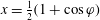 $x=\frac{1}{2}(1+\cos \unicode[STIX]{x1D711})$, and making use of the binomial theorem as well as the multiple angle formula of the sine and cosine functions, the transverse displacement of the inverted flag may be formulated as
 $$\begin{eqnarray}w(\unicode[STIX]{x1D711},t)=\mathop{\sum }_{i=1}^{M}p_{i}(t)\mathop{\sum }_{j=0}^{J_{i}}a_{i,j}\frac{1}{2^{j}}\mathop{\sum }_{m=0}^{j}\binom{j}{m}\cos ^{m}\unicode[STIX]{x1D711}.\end{eqnarray}$$
The perturbation pressure may be obtained analytically upon inserting (A 3) into (3.1), and applying Glauert’s integral equality (A 1) to perform integrations over  $\unicode[STIX]{x1D711}$. The resultant expression may be decomposed into three terms, associated with three effects of the pressure force in (3.1),
 $$\begin{eqnarray}\displaystyle \unicode[STIX]{x0394}p(\unicode[STIX]{x1D703},t) & = & \displaystyle \unicode[STIX]{x1D707}\mathop{\sum }_{i=1}^{M}\left(\ddot{p}_{i}(t)\int _{\unicode[STIX]{x1D703}}^{0}(\unicode[STIX]{x1D6F4}1_{i}-\unicode[STIX]{x1D6F4}2_{i})\,\text{d}\unicode[STIX]{x1D717}\right)+\unicode[STIX]{x1D6F1}^{2}\mathop{\sum }_{i=1}^{M}p_{i}(t)(\unicode[STIX]{x1D6F4}3_{i}-\unicode[STIX]{x1D6F4}4_{i}-\unicode[STIX]{x1D6F4}6_{i})\nonumber\\ \displaystyle & & \displaystyle -\,\unicode[STIX]{x1D6F1}\sqrt{\unicode[STIX]{x1D707}}\mathop{\sum }_{i=1}^{M}\left[{\dot{p}}_{i}(t)\left(\int _{\unicode[STIX]{x1D703}}^{0}(\unicode[STIX]{x1D6F4}3_{i}-\unicode[STIX]{x1D6F4}4_{i})\,\text{d}\unicode[STIX]{x1D717}+(\unicode[STIX]{x1D6F4}1_{i}-\unicode[STIX]{x1D6F4}2_{i}-\unicode[STIX]{x1D6F4}5_{i})\right)\right]\nonumber\\ \displaystyle & \equiv & \displaystyle \unicode[STIX]{x1D707}\mathop{\sum }_{i=1}^{M}\ddot{p}_{i}(t)P^{M}(\unicode[STIX]{x1D703})+\unicode[STIX]{x1D6F1}^{2}\mathop{\sum }_{i=1}^{M}p_{i}(t)P^{K}(\unicode[STIX]{x1D703})-\unicode[STIX]{x1D6F1}\sqrt{\unicode[STIX]{x1D707}}\mathop{\sum }_{i=1}^{M}{\dot{p}}_{i}(t)P^{C}(\unicode[STIX]{x1D703}),\end{eqnarray}$$
with  $P^{M}(\unicode[STIX]{x1D703})$,
 $P^{C}(\unicode[STIX]{x1D703})$ and
 $P^{K}(\unicode[STIX]{x1D703})$ being the components of
 $\unicode[STIX]{x0394}P(\unicode[STIX]{x1D703},t)$ obtained by retaining terms associated with
 $\ddot{p}_{i}(t)$,
 ${\dot{p}}_{i}(t)$ and
 $p_{i}(t)$ respectively. The values of
 $\unicode[STIX]{x1D6F4}1_{i}$–
 $\unicode[STIX]{x1D6F4}6_{i}$ are defined as
 $$\begin{eqnarray}\left.\begin{array}{@{}c@{}}\displaystyle \unicode[STIX]{x1D6F4}1_{i}=\mathop{\sum }_{j=1}^{J_{i}}a_{i,j}\frac{1}{2^{j}}\mathop{\sum }_{m=0}^{j}\binom{j}{m}2^{1-m}\mathop{\sum }_{n=0}^{(m-1)/2}\binom{m}{n}\unicode[STIX]{x1D6F4}1_{n},\\ \displaystyle \unicode[STIX]{x1D6F4}2_{i}=\mathop{\sum }_{j=1}^{J_{i}}a_{i,j}\frac{1}{2^{j}}\mathop{\sum }_{m=0}^{j}\binom{j}{m}\frac{1}{2^{m+1}}\mathop{\sum }_{n=0}^{(m-1)/2}\binom{m+2}{n}\unicode[STIX]{x1D6F4}2_{n},\\ \displaystyle \unicode[STIX]{x1D6F4}3_{i}=\mathop{\sum }_{j=1}^{J_{i}}a_{i,j}\frac{j}{2^{j-1}}\mathop{\sum }_{m=0}^{j}\binom{j-1}{m}2^{1-m}\mathop{\sum }_{n=0}^{(m-1)/2}\binom{m}{n}\unicode[STIX]{x1D6F4}1_{n},\\ \displaystyle \unicode[STIX]{x1D6F4}4_{i}=\mathop{\sum }_{j=1}^{J_{i}}a_{i,j}\frac{j}{2^{j-1}}\mathop{\sum }_{m=0}^{j}\binom{j-1}{m}\frac{1}{2^{m+1}}\mathop{\sum }_{n=0}^{(m-1)/2}\binom{m+2}{n}\unicode[STIX]{x1D6F4}1_{n},\\ \displaystyle \unicode[STIX]{x1D6F4}5_{i}=\mathop{\sum }_{j=0}^{J_{i}}a_{i,j}\frac{1}{2^{j}}\int _{0}^{\unicode[STIX]{x03C0}}(\cos \unicode[STIX]{x1D711}+1)^{j}(1-\cos \unicode[STIX]{x1D711})\,\text{d}\unicode[STIX]{x1D711},\\ \displaystyle \unicode[STIX]{x1D6F4}6_{i}=\mathop{\sum }_{j=0}^{J_{i}}a_{i,j}\frac{j}{2^{j-1}}\int _{0}^{\unicode[STIX]{x03C0}}(\cos \unicode[STIX]{x1D711}+1)^{j-1}(1-\cos \unicode[STIX]{x1D711})\,\text{d}\unicode[STIX]{x1D711},\end{array}\right\}\end{eqnarray}$$
where
 $$\begin{eqnarray}\left.\begin{array}{@{}c@{}}\displaystyle \unicode[STIX]{x1D6F4}1_{n}=\mathop{\sum }_{r=0}^{m-2n}\binom{m-2n}{r}\cos ^{r}\unicode[STIX]{x1D717}\sin ^{k-1}\unicode[STIX]{x1D717}\sin \left(k\frac{\unicode[STIX]{x03C0}}{2}\right),\\ \displaystyle \unicode[STIX]{x1D6F4}2_{n}=\mathop{\sum }_{r=0}^{m-2n+2}\binom{m-2n+2}{r}\cos ^{r}\unicode[STIX]{x1D717}\sin ^{k+1}\unicode[STIX]{x1D717}\sin \left((k+2)\frac{\unicode[STIX]{x03C0}}{2}\right),\end{array}\right\}\end{eqnarray}$$
and  $k=m-2n-r$.
Hence, integrations over  $\unicode[STIX]{x1D711}$ are performed exactly and the pressure distribution over the inverted flag may be evaluated analytically. Applying the Galerkin technique to (3.1) yields
 $$\begin{eqnarray}\left.\begin{array}{@{}c@{}}\displaystyle M_{ij}=\int _{0}^{\unicode[STIX]{x03C0}}{\textstyle \frac{1}{2}}(\unicode[STIX]{x1D707}P_{i}^{M}(\unicode[STIX]{x1D703})+W_{i}(\unicode[STIX]{x1D703}))W_{j}(\unicode[STIX]{x1D703})\sin \unicode[STIX]{x1D703}\,\text{d}\unicode[STIX]{x1D703},\\ \displaystyle C_{ij}=-\unicode[STIX]{x1D6F1}\sqrt{\unicode[STIX]{x1D707}}\int _{0}^{\unicode[STIX]{x03C0}}{\textstyle \frac{1}{2}}P_{i}^{C}(\unicode[STIX]{x1D703})W_{j}(\unicode[STIX]{x1D703})\sin \unicode[STIX]{x1D703}\,\text{d}\unicode[STIX]{x1D703}+\unicode[STIX]{x1D702}_{s}\int _{0}^{1}\unicode[STIX]{x2202}_{xxxx}W_{i}(x)W_{j}(x)\,\text{d}x,\\ \displaystyle K_{ij}=\unicode[STIX]{x1D707}\int _{0}^{\unicode[STIX]{x03C0}}{\textstyle \frac{1}{2}}P_{i}^{K}(\unicode[STIX]{x1D703})W_{j}(\unicode[STIX]{x1D703})\sin \unicode[STIX]{x1D703}\,\text{d}\unicode[STIX]{x1D703}+\int _{0}^{1}\unicode[STIX]{x2202}_{xxxx}W_{i}(x)W_{j}(x)\,\text{d}x.\end{array}\right\}\end{eqnarray}$$
For the nonlinear analysis, the following comparison functions are defined by their polynomial successors to discretize the nonlinear equation of motion (2.24):
 $$\begin{eqnarray}\unicode[STIX]{x1D6F9}_{i}(x)=\sin (\unicode[STIX]{x1D706}_{i}x)+\sinh (\unicode[STIX]{x1D706}_{i}x)+\frac{\cos (\unicode[STIX]{x1D706}_{i})+\cosh (\unicode[STIX]{x1D706}_{i})}{\sin (\unicode[STIX]{x1D706}_{i})+\sinh (\unicode[STIX]{x1D706}_{i})}(\cos (\unicode[STIX]{x1D706}_{i}x)-\cosh (\unicode[STIX]{x1D706}_{i}x)),\end{eqnarray}$$
recalling that  $\unicode[STIX]{x1D706}_{i}$ is the
 $i$th root of the transcendental equation
 $1+\cosh (x)\cos (x)=0$ (Bishop & Johnson Reference Bishop and Johnson2011). These functions are suitable since they satisfy the clamped–free boundary conditions, and also convenient, as they are already known (note that
 $\unicode[STIX]{x1D713}(x,t)=\unicode[STIX]{x2202}_{x}w(x,t)$ holds for the linear equation of motion of the flag; hence
 $\unicode[STIX]{x1D6F9}_{i}(x)=\unicode[STIX]{x2202}_{x}W_{i}(x)$ are chosen). Similarly to (A 2), polynomial representations of these comparison functions are constructed with the aid of Chebyshev polynomial expansions of the first kind with a sufficiently large number of terms (i.e.
 $\unicode[STIX]{x1D6F9}_{i}(x)=\sum _{j=1}^{J_{i}}a_{ij}jx^{j-1}$). The first six comparison functions are shown in figure 20.
First six in vacuo comparison functions of a cantilevered beam utilized in the Galerkin discretization of the nonlinear system. First (red), second (light brown), third (brown), fourth (black), fifth (blue) and sixth (light blue) comparison functions.

It is clear from (2.3) that the normal component of the relative velocity is a function of trigonometric expressions in terms of  $\unicode[STIX]{x1D713}(x,t)$. For the problem at hand, retaining these trigonometric terms intact hinders the evaluation of the exact solution of the non-circulatory velocity potential, by virtue of the fact that the integral is singular and hence its principal value needs to be calculated. In order to overcome this difficulty, the normal component of the relative velocity is expressed in a succession of Taylor’s expansions. This results in a polynomial representation of the source/sink sheet strength in terms of the rotation angle. Hence,
 $$\begin{eqnarray}\displaystyle V_{n}(x,t) & {\approx} & \displaystyle -\unicode[STIX]{x1D6F1}\sqrt{\unicode[STIX]{x1D707}}\left[\unicode[STIX]{x2202}_{t}\left(\int _{0}^{x}\mathop{\sum }_{r=1}^{R}\frac{(-1)^{r}}{(2r)!}\unicode[STIX]{x1D713}(s,t)^{2r}\,\text{d}s\right)+1\right]\mathop{\sum }_{r=1}^{R}\frac{(-1)^{r}}{(2r+1)!}\unicode[STIX]{x1D713}(x,t)^{2r+1}\nonumber\\ \displaystyle & & \displaystyle +\,\unicode[STIX]{x1D6F1}\sqrt{\unicode[STIX]{x1D707}}\mathop{\sum }_{r=1}^{R}\frac{(-1)^{r}}{(2r)!}\unicode[STIX]{x1D713}(x,t)^{2r}\unicode[STIX]{x2202}_{t}\left(\int _{0}^{x}\mathop{\sum }_{r=1}^{R}\frac{(-1)^{r}}{(2r+1)!}\unicode[STIX]{x1D713}(s,t)^{2r+1}\,\text{d}s\right),\end{eqnarray}$$
where  $R$ is the order of truncation. Similarly to the procedure detailed earlier, inserting
 $\unicode[STIX]{x1D6F9}_{i}(x,t)=\sum _{i=1}^{M}q_{i}(t)(\sum _{j=1}^{J_{i}}a_{ij}jx^{j-1})$ into (A 9), the velocity potential given in (2.13) can be integrated based on Glauert’s integral. This enables the analytical evaluation of the pressure distribution over the flag, in a similar fashion to the discretization technique detailed for the linear model. In this paper, terms up to third order are retained in the Taylor expansions in (A 9), resulting in
 $$\begin{eqnarray}\displaystyle V_{n}(x,t) & {\approx} & \displaystyle \unicode[STIX]{x1D6F1}\sqrt{\unicode[STIX]{x1D707}}\left[\unicode[STIX]{x1D713}(x,t)\int _{0}^{x}\dot{\unicode[STIX]{x1D713}}(s,t)\unicode[STIX]{x1D713}(s,t)\,\text{d}s+(1-{\textstyle \frac{1}{2}}\unicode[STIX]{x1D713}(x,t)^{2})\int _{0}^{x}\dot{\unicode[STIX]{x1D713}}(s,t)\,\text{d}s\right.\nonumber\\ \displaystyle & & \displaystyle -\left.{\textstyle \frac{1}{2}}\int _{0}^{x}\dot{\unicode[STIX]{x1D713}}(s,t)\unicode[STIX]{x1D713}(s,t)^{2}\,\text{d}s\right]-\unicode[STIX]{x1D713}(x,t)+{\textstyle \frac{1}{6}}\unicode[STIX]{x1D713}(x,t)^{3}.\end{eqnarray}$$