Introduction
The transformation of deep water rice (DWR) to flooded rice (FDR) production systems prompted the need for practical and reliable recommendations for farmers to fully adapt to the newly introduced system. Recommendations can be generated under a series of field experiments and subsequently demonstrated or disseminated to farmers. However, field experiments are expensive and time-consuming (Kundu et al., Reference Kundu, Skogerboe and Walker1982; Knörzer et al., Reference Knörzer, Grözinger, Graeff-Hönninger, Hartung, Piepho and Claupein2011). Crop simulation models have been developed based on the theory of crop physiological ecology (Graves et al., Reference Graves, Hess, Matthews, Stephens and Middleton2002). They are dynamic in the mechanism, comprehensiveness and applicability, and can be used to simulate the interaction of weather, soil, genotype and crop management on crop growth and yield (Jones et al., Reference Jones, Hoogenboom, Porter, Boote, Batchelor, Hunt, Wilkens, Singh, Gijsman and Ritchie2003; Jiang and Jin, Reference Jiang and Jin2009). The concept of crop development mainly involves crop phenology, leaf age increment and appearance of various organs such as leaf blades, leaf sheaths, tillers, roots, stem internodes and panicles (Ritchie et al., Reference Ritchie, Alocilja, Singh and Uehera1987; Gao et al., Reference Gao, Jin, Huang and Zhang1992).
Crop simulation models have been used widely to describe systems and processes at various levels of agricultural systems from genotype, crop and farming system levels up to regional and global environment levels (Matthews et al., Reference Matthews, Stephens, Hess, Middleton and Graves2002). There have been various applications of the Cropping System Model-Crop Environment Resource Synthesis-Rice (CSM-CERES-Rice) model in Asia such as yield gap and yield trend analysis to improve overall crop management by making appropriate planting decisions, devising improved cultural practices, developing fertilizer use efficiency, water and pest management (Timsina and Humphreys, Reference Timsina and Humphreys2006b). The model was also applied to assess the impact of climate change on rice productivity to assist policymakers with strategic decision-making and planning (Timsina and Humphreys, Reference Timsina and Humphreys2006a; Yao et al., Reference Yao, Xu, Lin, Yokozawa and Zhang2007; Jintrawet and Chinvanno, Reference Jintrawet and Chinvanno2011). However, the ultimate goal of using a crop model would be beneficial for small-scale resource-poor households who are dependent upon crop production for their livelihoods. Therefore, there is an urgent need to evaluate the model in research more relevant to problems in the real world and to find effective alternative technology to overcome existing problems for those beneficiaries. This means that researchers must consider the real problems facing farmers in these regions, and evaluate and apply these models to contribute to solving local problems for small-holder farmers (Matthews et al., Reference Matthews, Stephens, Hess, Middleton and Graves2002). The advantage of decision support systems and crop simulation models is that these tools can reduce the need for expensive and time-consuming field experimentation and can be used to analyse yield gaps for various cropping systems including rice. However, proper calibration and evaluation in the environment of interest before applying them to evaluate management options must be done. This is especially important in the absence of reports on the evaluation of model processes as reflected in the models’ relative inabilities to predict a range of crop, soil and water parameters (Timsina and Humphreys, Reference Timsina and Humphreys2006a).
The CSM-CERES-Rice model of DSSAT Version 4.0.2.0 was calibrated and evaluated using the data from a field experiment carried out during the rainy season of 2004/05 at Shalimar, Srinagar (1587 m asl), India (Singh et al., Reference Singh, Singh and Hasan2007). A crop-growth simulation model, CERES-Rice, was applied to 16 locations representing major rice-growing regions of Bangladesh to determine baseline yield estimates for four transplanting dates (Mahmood et al., Reference Mahmood, Meo, David and Mark2003). Moreover, testing of the CERES-Rice model by statistical analysis and application confirmed that this model could be acceptable for use as a research tool to choose the most appropriate strategy prior to conducting field experiments (Cheyglinted et al., Reference Cheyglinted, Ranamukhaarachchi and Singh2001).
There are four different input data sets required for the evaluation and application of the cropping system model (CSM) of DSSAT including soil data, weather data, management data and crop characteristics data or crop genetic coefficients (GC) (Hoogenboom et al., Reference Hoogenboom, Jones, Porter, Wilkens, Boote, Hunt and Tsuji2013). In the past, crop modellers have used two techniques to calculate the GC of a rice variety for known crop development and growth of a particular experiment. The first method is by trial-and-error and the second is a calculation technique such as the GC calculator (GENCALC), which uses a deterministic stepwise procedure to automatically adjust the coefficients with values within the plant's realistic physiological ranges (Hunt et al., Reference Hunt, Pararajasingham, Jones, Hoogenboom, Imamura and Ogoshi1993; Pabico, Reference Pabico2008). GENCALC has been used successfully for the estimation of GC for peanut (Anothai et al., Reference Anothai, Patanothai, Jogloy, Pannangpetch, Boote and Hoogenboom2008), soybean (Bao et al., Reference Bao, Hoogenboom, McClendon and Paz2015) and maize (Bao et al., Reference Bao, Hoogenboom, McClendon and Vellidis2017).
Generalized likelihood uncertainty estimation (GLUE) has been used extensively in the field of hydrological modelling. It is a Bayesian estimation method that uses Monte Carlo sampling from prior distributions of the coefficients and a Gaussian likelihood function to determine the best coefficients based on the data that are used in the estimation process. The version of GLUE implemented in DSSAT was developed by He et al. (Reference He, Jones, Graham and Duke2010a, Reference He, Porter, Wilkens, Marin, Hu, Jones, Jones, Hoogenboom, Wilkens, Porter and Tsuji2010b). Based on known information, the distribution for each individual GC has been defined (prior distribution). GLUE is then applied to the simulation of one or more treatments and a new distribution for each individual GC is determined (posterior distribution). In DSSAT, the GC for the development processes are estimated first, followed by the GC for growth, yield and yield components.
Both GENCALC and GLUE were included in DSSAT Version 4.5 (Hoogenboom et al., Reference Hoogenboom, Jones, Wilkens, Porter, Boote, Hunt, Singh, Lizaso, White, Uryasev, Royce, Ogoshi, Gijsman and Tsuji2011). There are advantages and disadvantages of using these estimators. One disadvantage of the GLUE program is that it requires a lot of computation time, depending on the number of treatments selected for the estimation process and the complexity of the GC for a particular crop module in DSSAT (He et al., Reference He, Porter, Wilkens, Marin, Hu, Jones, Jones, Hoogenboom, Wilkens, Porter and Tsuji2010b). On the other hand, GENCALC requires more manual operation than GLUE.
The overall goal of the current study was to evaluate the performance of two different methods for estimating GC of FDR with the CSM-CERES-Rice model. The specific objectives were to determine the GC for a field experiment designed to study the effect of planting date and variety of FDR production system in a deep water area in Thailand and to compare simulated and observed phenology, yield and yield components for this experiment. The hypothesis was that the best GC estimator could be used to assist with providing recommendations to farmers to adapt and change to FDR production system in deep water area based on a modelling and systems analysis approach.
Materials and methods
Field experiment
A field experiment was conducted at the Bang Tean His Majesty's Private Development Project, Bansang, Prachin Buri, Thailand (13°52′N, 101°09′E, 2 m asl). The experimental design was a split-plot consisting of four planting dates and three rice varieties as main plot and sub-plot, respectively, with four replications. The four planting dates were 19 June, 12 July, 16 July and 23 July 2009. The rice varieties were Chai Nat 1 (CNT1), Pathum Thani 1 (PTT1) and Pitsanulok 2 (PSL2). These are all non-photosensitive rice varieties (Rice Department, 2009). The planting method was transplanting at a spacing of 20 × 20 cm2 with three seedlings per hill. The area of the main plot was 7.0 × 8.8 m2 with three sub-plots measuring 7.0 × 2.8 m2. The border between each main plot was 1 m. Each sub-plot contained 15 rows with 36 hills per row. Continuous flooding was maintained at a depth of 10 cm during the growing season. There were two applications of chemical fertilizer; the first applied at a rate of 30 kg nitrogen (N) and 36 kg phosphorus pentoxide (P2O5)/ha about 1 week after transplanting and the second applied at a rate of 29 kg N/ha at the panicle initiation (PI) development stage (growth stage (GS) 30 according to Meier, Reference Meier2001) of the three rice varieties (Department of Agriculture, 2004a, 2004b).
Data collection
The calibration and evaluation of the model requires crop management, weather, soil characteristics and genotype characteristics data as follows (Hunt and Boote, Reference Hunt, Boote, Tsuji, Hoogenboom and Thornton1998; Hunt et al., Reference Hunt, White and Hoogenboom2001);
(1) The data sets for model operation consist of:
– Description of field experiment site: Latitude, longitude, elevation and slope as above
– Weather data: Maximum and minimum temperature, precipitation and solar radiation on a daily basis
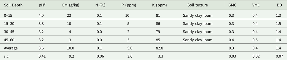
– Soil data: Soil analysis by layer, bulk density, organic carbon, organic nitrogen, pH, phosphorus (P) and potassium (K) (Table 1)
Table 1.Soil chemical and physical properties of the experimental site, Prachin Buri, Thailand, 2009

OM, organic matter; N, total nitrogen; P, available phosphorus; K, extractable potassium; GMC, gravimetric moisture content; VMC, volumetric moisture content; BD, soil bulk density; s.d., standard deviation.
a pH: 1:1 (H2O).
– Initial condition: Biomass of the previous crop
– Crop management: Rice cultivar, planting date, planting method, spacing and plant population
– Irrigation and water management
– Fertilizer management: Product, time and amount of application and method of application
(2) Rice crop performance: PI, flowering, milky ripe and harvesting dates, yield and yield components, and percentage of leaf N in crop biomass.

Biomass sampling for growth measurement and dates of phenology development were collected throughout the growing season (Buddhaboon et al., Reference Buddhaboon, Jintrawet and Hoogenboom2011; Hoogenboom et al., Reference Hoogenboom, Jones, Porter, Wilkens, Boote, Hunt and Tsuji2013). A rice plant has three major developmental phases: vegetative phase, the reproductive phase and ripening phase (Department of Agriculture, 2004a). The vegetative phase covers the period from germination (GS 05) to PI (GS 30). The reproductive phase covers the period from PI to flowering (GS 61) and the ripening phase (GS 89) covers the period from flowering (GS 61) to maturity (GS 89) (Meier, Reference Meier2001). The developmental stages and associated dates were monitored, including the PI date, flowering date, the milky ripe date and the maturity or harvest date. The PI date was monitored daily starting at 55 days after transplanting until the appearance of the panicle primordium. For the other developmental stages, a 5-day interval was used for monitoring. Biomass samples for growth analysis were collected throughout the growing season (Hoogenboom et al., Reference Hoogenboom, Jones, Porter, Wilkens, Boote, Hunt and Tsuji2013). Rice biomass and yield samples were collected five times, including at the seedling stage (GS 13, during the vegetative phase), PI stage (GS 30), flowering stage (GS 61), milky stage (GS 73) and maturing stage (GS 89) (Meier, Reference Meier2001; Department of Agriculture, 2004a). One hundred plants for each variety were collected at the seedling stage before transplanting. For the PI stage, flowering stage and milky ripe stage, 15 hills per plot were sampled. At final harvest, 40 hills were sampled for biomass, yield and yield component analysis. The individual stem, leaf and panicle components of the sampled rice hills were separated and dried in a fan-assisted oven at 75 °C for 72 h until constant weight.
Input file preparation
Five input files were created for running the DSSAT V4.5 CSM-CERES-rice model: FileX, FileA, FileT, Soil file and Weather file. FileX, or the management file, stored data of field conditions, field management, treatments in the experiment and simulation option. The existing field environment indicated weather data, soil properties and initial condition of the field. The major part of FileX is crop production management data, separated into various sections, for example, rice cultivar, planting detail, irrigation method, fertilizer application (organic and inorganic fertilizer), tillage, harvest and chemical application sections. In addition, the simulation option section served as a model calculation control. It defined the start simulation date, provided options to activate water and/or N modules and method of calculation for weather, soil water balance and photosynthesis. The output can also be framed under the simulation option section. The treatment section in FileX is a combination of environment, management and simulation options.
FileA and FileT are designed to store selected field experimental observations related to rice phenology and growth processes which can be compared with the simulated values as well as used to estimate GC. FileA stores values of selected observations of each treatment in the experiment at harvest, while FileT stores time series values at a given phenological stage, observed during the growing season of each treatment.
The soil input file contains physical and chemical soil properties of the field experiment plot. Composite soil samples were collected from four layers: 0–15, 15–30, 30–45 and 45–60 cm depth (Table 1). Most rice roots grow in the top layer. Soil pH, organic matter, total N, available P, extractable K and soil bulk density were analysed in laboratory based on standard methods (Bray and Kurtz, Reference Bray and Kurtz1945; Jackson, Reference Jackson1965; Pratt, Reference Pratt and Black1965). Biomass from the previous crop was also collected at the same time as soil sampling, 7 days prior to ploughing. The amount of previous crop biomass in the experimental field was 3725 kg/ha. The analysed data of soil samples and previous crop biomass were used to create the soil file and soil analysis and initial condition in FileX.
Daily weather data were obtained from the Prachin Buri Meteorology Station, located at 14°3′N, 101°22′E. Precipitation data were also collected by the Bang Tean His Majesty's Private Development Project. The two locations were located in the same DWR area, at the same altitude of 2 m asl and with no mountain ranges in the area. The observed weather data set consisted of precipitation, maximum and minimum temperature. Solar radiation was calculated using the minimum and maximum temperature (Hunt et al., Reference Hunt, Kuchar and Swanton1998; Phakamas et al., Reference Phakamas, Jintrawet, Patanothai, Sringam and Hoogenboom2013).
Genetic coefficient calculation
The GC for the three FDR varieties were estimated by using two GC calculator modules in the DSSAT V4.5 packages, GC calculator (GENCALC) and GLUE.
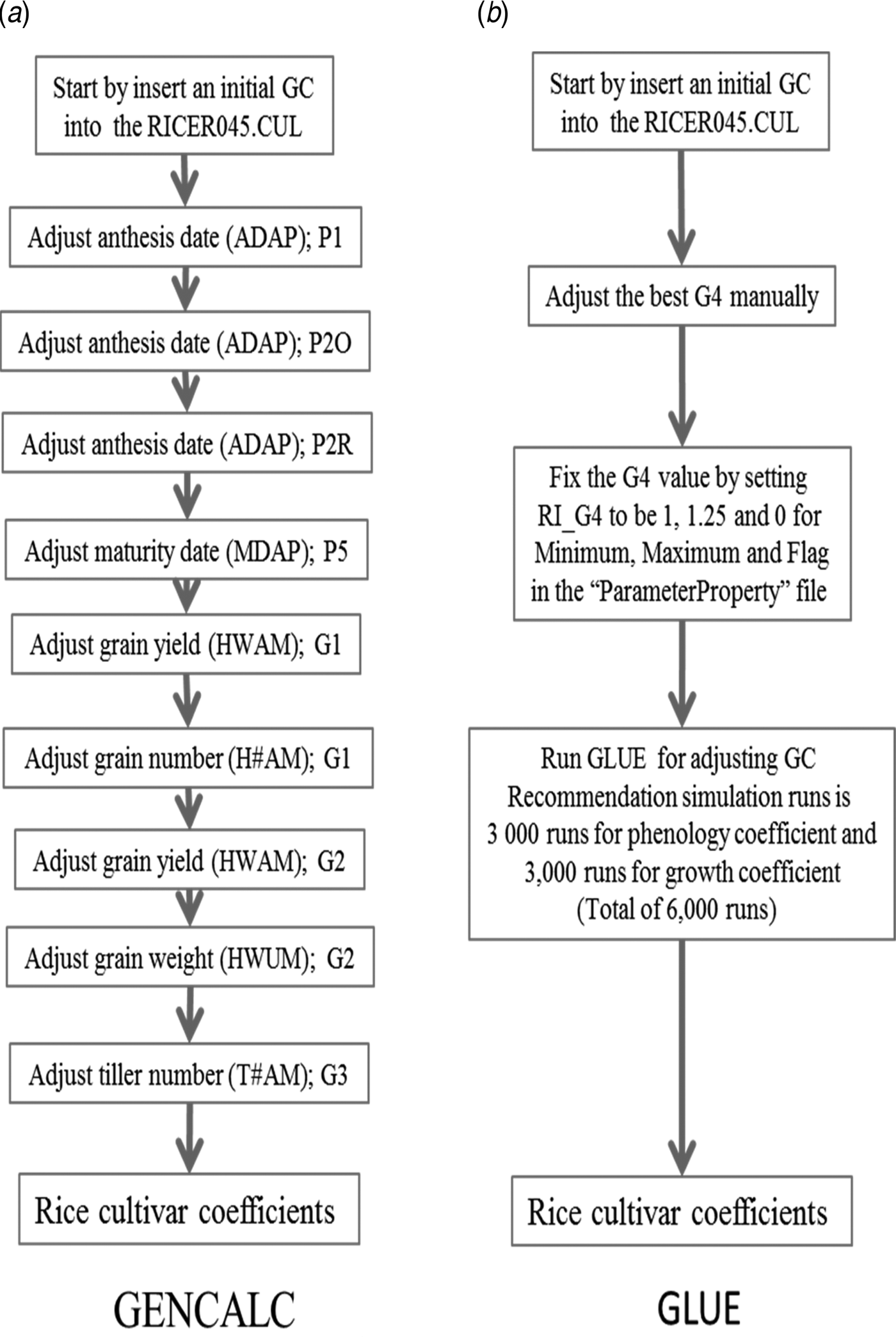
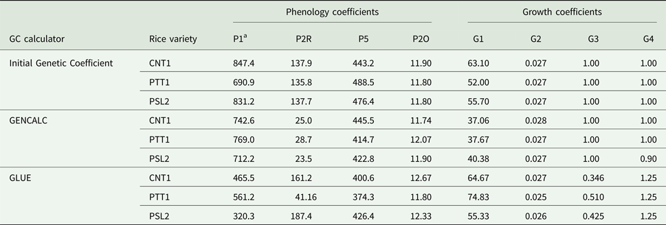
The GENCALC calculation for GC (Table 2) of the three rice varieties started with a set of the same initial cultivar coefficients as those used in GLUE GC. The rice model was defined by the user to perform step-by-step calculations for each coefficient. Beginning with the P1 coefficient, which controls anthesis date (anthesis days after planting), GENCALC searched the output file from the crop model and adjusted the P1 coefficient to produce the lowest RMSE between the simulated and observed dates to the anthesis dates (Wallach and Goffinet, Reference Wallach and Goffinet1987). The coefficient could be increased or decreased for optimization to minimize the RMSE between observed and simulated values. The new coefficients could be inserted automatically or manually into rice genetic cultivar file. The calculation was repeated using the newly inserted coefficient until the minimum value for RMSE and normalized root mean square error (RMSEn) was obtained (Wallach and Goffinet, Reference Wallach and Goffinet1987; Loague and Green, Reference Loague and Green1991). The same procedure was repeated to determine the values for P2O, P2R, P5 G1, G2 and G3 coefficients, respectively (Fig. 1(a)). After the final run of the GC calculation, the new set of GC for the new rice variety was obtained based on the experimental data set.
The sequence of optimizations for calibrating the cultivar coefficients using GENCALC (a) and GLUE GC (b) estimators.

Abbreviations, definitions and units of the eight rice genetic coefficients of the CSM-CERES-Rice model

The interface for the GLUE program in DSSAT can be accessed from the DSSAT tool menu to start the procedure (He et al., Reference He, Jones, Graham and Duke2010a, Reference He, Porter, Wilkens, Marin, Hu, Jones, Jones, Hoogenboom, Wilkens, Porter and Tsuji2010b). The user selects a crop and the cultivar for which the GC will be estimated. For the selected treatments from one or more experiments, the Monte Carlo method provides the maximum likelihood estimation (MLE) for the phenological development and growth GC (He et al., Reference He, Porter, Wilkens, Marin, Hu, Jones, Jones, Hoogenboom, Wilkens, Porter and Tsuji2010b). Maximum likelihood estimation is the preferred method for parameter estimation in statistics and has been a useful tool for many statistical modelling techniques, especially for non-linear modelling with non-normal data. It was based on the principle that the desired probability distribution is the one that makes the observed data ‘most likely’, which means that one must seek the value of the parameter vector that maximizes the likelihood function (Myung, Reference Myung2003). Among the eight rice GC of the CSM-CERES-Rice model, the G4 coefficient affects all others and was fixed at 1.25, before setting the GLUE program to run for all parameters of each variety. Recommendations for the number of simulations required for the GLUE estimator to obtain the best GC are 6000 simulations, e.g. 3000 simulation runs for the phenological coefficients and another 3000 simulations for the growth coefficients (Fig. 1(b)). However, this also depends on the complexity of the experimental input data sets (He et al., Reference He, Porter, Wilkens, Marin, Hu, Jones, Jones, Hoogenboom, Wilkens, Porter and Tsuji2010b).
Rice growth, development and yield simulation
The calibrated GC values of three rice cultivars used the two GC estimators to run the CSM-CERES-Rice model of DSSAT Version 4.5 for simulating rice development, growth and yield for different planting dates of FDR production before flooding in a deep water area. The simulated development, growth, yield and crop N uptake were compared with observed data.
Data analysis
The RMSE, RMSEn, r 2 and index of agreement (D-index or D-stat) statistics were used to compare the simulated data with observed values. The RMSE was used to compare the difference between the simulated data of the crop simulation model with the observed data from the field experiment. The model reproduced experimental data perfectly when RMSE value was 0. The calculation was made using the following formula:
 $$RMSE = \left[ {N^{ - 1}\mathop \sum \limits_{i = 1}^n {(\,p_i - o_i)}^2} \right]^{0{\cdot}5}\; $$
where p i is simulated value, o i is observed value and N is number of observation (equal to the number of simulation; Wallach and Goffinet, Reference Wallach and Goffinet1987; Timsina and Humphreys, Reference Timsina and Humphreys2006a).
The RMSEn was computed for each parameter to compare the outputs from simulation against observation data via the following equation:
 $$RMSEn = \displaystyle{{RMSE \times 100\;} \over {\bar o}}\; $$
where  $\bar o$ is the overall mean of observation values (Loague and Green, Reference Loague and Green1991).
The D-index or D stat, a descriptive (both relative and bounded) measure, was applied to calculate the agreement between observed and simulation. It has values between zero and one, with one being the best fit (Timsina and Humphreys, Reference Timsina and Humphreys2006a; Anothai et al., Reference Anothai, Patanothai, Jogloy, Pannangpetch, Boote and Hoogenboom2008). The formula to calculate the D-index is shown below:
 $$D - index = 1 - \left[ {\mathop \sum \limits_{i = 1}^n {(\,p_i - o_i)}^2/\mathop \sum \limits_{i = 1}^n {\left( {\left \vert {\,p_i^{\prime}} \right \vert + \left \vert {o_i^{\prime}} \right \vert} \right)}^2} \right]\; $$
where  $p_i^{\prime} $ =
 $p_i - \bar o$ and
 $o_i^{\prime} $ =
 $o_i - \bar o$.
The r 2 value ranges from 0 (the proposed model does not fit at all) to 1 (proposed model fits the data perfectly). The calculation was made using the following equation:
 $$r^2 = 1 - \displaystyle{{\mathop \sum \nolimits_i {(O_{i\;} - \; p_i)}^2} \over {\mathop \sum \nolimits_i {(O_{i\;} - \; \bar o\; )}^2}}\; $$
where o i is the ith observation of parameter o; p i is the ith simulation of parameter p;  $\bar o$ is arithmetic mean of parameter o (Kammen and Hassenzahl, Reference Kammen and Hassenzahl2001).
Results
Genetic coefficients of flooded rice variety
Eight GC of three FDR varieties, Chai Nat 1, Pathum Thani 1, and Pitsanulok 2, were determined using the GENCALC and GLUE GC estimators. The GC for rice phenology and growth were calculated. The phenology coefficients were P1, P2O, P2R and P5, while the growth coefficients were G1, G2, G3 and G4 (Table 2). The GC for the same rice variety determined with the GENCALC and GLUE GC estimators showed a difference for both the phenology and growth coefficients. The P1 coefficient values of GENCALC were higher than GLUE and significant at P < 0.016, while the P2R coefficients of GENCALC were lower than GLUE, but not significant. Likewise, the G3 coefficients of GENCALC were higher than GLUE and the G4 coefficient of GENCALC were lower than GLUE, both were not significant (Table 3). However, these two different sets of rice GC gave similar simulated values for the developmental and growth variables when compared with the observed values of FDR under deep water area condition in Thailand.
Initial and final values of the genetic coefficients for three flooded rice varieties calculated with the GENCALC and GLUE GC estimators under different planting dates of flooded rice production in deep water rice area, Prachin Buri, Thailand, 2009

GC, genetic coefficients.
a See Table 2 for explanation of acronyms for phenology and growth coefficients.
Phenology simulation
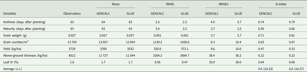
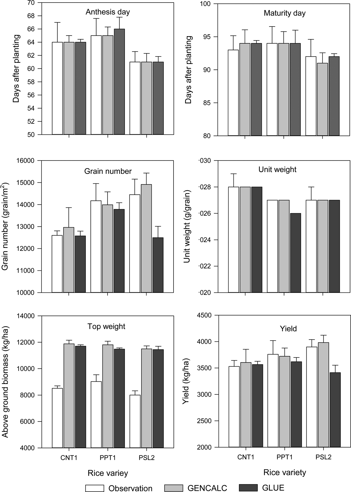
Two critical development phases of FDR to compare with observed data were the anthesis and maturity dates. The observed average duration of development phases across varieties and planting dates was 63 and 93 days after transplanting for anthesis and maturity, respectively. For estimated values, the outputs for anthesis and maturity using GENCALC GC were 64 and 93 days, respectively, and 63 and 93 days after planting, respectively, using GLUE. The RMSEn values for the two stages were 3.97 and 3.67, and 3.67 and 2.50 for GENCALC and GLUE, respectively. Both simulation results were satisfactory (RMSEn < 10) compared with the observed data (Table 4). Duration of growth from transplanting to harvest was the same at 93 days for both simulations and observations.
A comparison between simulated anthesis and flowering dates and yield and yield components with GENCALC and GLUE GC comparison with observed for flooded rice production in the deep water area, Prachin Buri, Thailand, 2009

RMSE, root mean square error; RMSEn, normalized root mean square error; D-index, index of agreement.
Growth and yield simulation
Three growth variables were selected for comparison of the two GC estimators with observed data: grain weight, grain number (Table 3) and above-ground biomass (Fig. 2). The overall grain weight was simulated precisely by both sets of GC when compared with field observations. The overall average grain weight was 0.027 g/grain (RMSEn = 3.68) for both GENCALC and GLUE, which was the same as observed values. Observed grain number/m2 was 13 743 while GENCALC and GLUE GC outputs were 13 957 and 12 945, respectively, with RMSEn values of 8.29 and 10.38, respectively (Table 4). GENCALC GC showed good agreement with observed values for grain number/m2 while GLUE GC showed fairly good agreement. Observed grain yield was 3729 kg/ha compared with 3769 and 3532 kg/ha for simulation outputs using GENCALC GC and GLUE GC, respectively. Therefore, the GENCALC GC seems to be better than the GLUE GC in terms of simulating rice yield. However, above-ground biomass was over-estimated by >3 t/ha by both GENCALC and GLUE GC (Table 4). In addition, the simulated leaf N (%) results showed good agreement (D-Index) and high correlations (R 2) between observed and simulated values, with high RMSEn values (Table 4, Fig. 3 and Fig. 4).
Observed and simulated stem weight, leaf weight, above-ground biomass and grain weight of Chai Nat 1 (CNT1), Pathum Thani 1 (PTT1) and Pitsanulok 2 (PSL2) from four planting dates (PD1: June 19, PD2: July 2, PD3: July 16 and PD4: July 23) using genetic coefficient estimated by GENCALC and GLUE estimators, Prachin Buri, Thailand, 2009.

Observed and simulated leaf nitrogen (%) of Chai Nat 1 (CNT1), Pathum Thani 1 (PTT1) and Pitsanulok 2 (PSL2) from four planting dates (PD1: 19 June, PD2: 2 July, PD3: 16 July and PD4: 23 July) using genetic coefficient estimated by GENCALC and GLUE estimators, Prachin Buri, Thailand, 2009.

Observed and simulated anthesis date, maturity date, grain number, unit weight (grain weight: gram/grain), top weight (above-ground biomass) and yield of Chai Nat 1 (CNT1), Pathum Thani 1 (PTT1), and Pitsanulok 2 (PSL2) from four planting dates (PD1: 19 June, PD2: 2 July, PD3: 16 July and PD4: 23 July) using genetic coefficient estimated by GENCALC and GLUE GC estimators, Prachin Buri, Thailand, 2009.

Comparison of anthesis date, maturity date, grain number, grain weight, yield and above-ground biomass under GENCALC and GLUE GC found that there were no significant differences between simulation under two GCs and observed values in term of anthesis date, maturity date and grain weight. However, grain number and yield simulated using the GLUE GC were less than observed and simulated values under GENCALC GC. Simulated above-ground biomass for the three varieties was over-estimated significantly, P = 0.009 (Fig. 4). The average D-index values of all GC were 0.6 (±0.23) and 0.6 (±0.27) under GENCALC and GLUE GC estimators, respectively. These indicated similarities between the simulated values from the GC under GENCALC and the GLUE GC estimators (Table 4).
Discussion
Rice GC were separated into two groups including the phenology coefficients and growth coefficients. GLUE was more accurate than GENCALC with respect to estimating the phenology GC, while GENCALC was more accurate than GLUE for estimating growth GC, based on the D-index. The most influential rice GC affecting other coefficients, both phenology and growth coefficients, was the G4 coefficient. The GENCALC method did not calibrate for the G4 coefficient; the value for G4 is fixed at 1.0 for varieties grown in a normal environment, while the value for G4 is <1.0 for indica-type rice grown in very cool environments or seasons (Hoogenboom et al., Reference Hoogenboom, Jones, Porter, Wilkens, Boote, Hunt and Tsuji2013). In GLUE GC, the G4 value was fixed as 1.25 and proceeded to run automatically within the defined ranges for all phenology and growth GC (He et al., Reference He, Jones, Graham and Duke2010a, Reference He, Porter, Wilkens, Marin, Hu, Jones, Jones, Hoogenboom, Wilkens, Porter and Tsuji2010b). Alternatively, the user may define the Maximum, Minimum and Flag values of G4 in the ‘ParameterProperty’ file of DSSAT and set to 1.25, 1.0 and 0.0, respectively.
One advantage of the GENCALC estimator is that it is less time-consuming compared with the GLUE estimator. The disadvantages are that the user's skill is needed and that the calculation of GC is based on a sequential manual operation, step by step from P1 to G3 coefficient, until the best GC are obtained with a minimum RMSE, RMSEn and D-stat when the simulated values are compared with the observed data. The GLUE estimator is run automatically for more than 6000 iterations, which can be time-consuming. In addition, the value for G4 must be defined manually and fixed prior to run the GLUE estimator for obtaining the best GC.
The simulated above-ground biomass was over-estimated by both GC inputs, partially due to issues with leaf and stem biomass towards the end of the growing season. However, the overall anthesis and maturity dates, grain weight, grain yield and leaf N (%) simulation outputs based on the GENCALC and GLUE GC were not significantly different and there was a good agreement with the observed values.
Conclusion
The calibration of the rice GC calibration using GENCALC and GLUE GC estimators included in DSSAT Version 4.5 resulted in simulated anthesis, maturity dates and grain weight with RMSEn of 3.97, 3.69 and 3.68, respectively, for the GENCALC GC and at RMSEn of 3.67, 2.50 and 3.68, respectively for the GLUE GC. The simulated and observed grain number and grain yield for the GENCALC GC were not significantly different, but their values were slightly higher than the simulated values for the GLUE GC. The simulated values for above-ground biomass for both GENCALC (11 727 kg/ha) and GLUE GC (11 544 kg/ha) were over-estimated compared with the observed data (8512 kg/ha). The current study showed the capability of GENCALC and GLUE to estimate the GC for three flooded rice cultivars grown in the DWR area in Thailand. Future applications of both GC estimators for other rice varieties are need as an efficient way to promote the implementation of crop simulation models in Thailand and Southeast Asia region for the evaluation of various rice production options.
Acknowledgements
The interface for the GLUE and GENCALC programs in DSSAT were designed and programmed by Dr Paul Wilkens. We appreciate the assistance of staff at the Prachin Buri Rice Research Center, Rice Department Thailand, who conducted the field experiment. Technical and crop modelling support was provided the Department of Biological and Agricultural Engineering, University of Georgia, USA and the AgWeatherNet Program at Washington State University, USA.
Financial support
Financial support for this research was provided by The Thailand Research Fund (TRF) grant number RDG51O0004-DSSPHD/001/2551.
Conflict of interest
The authors have no conflict of interest to declare.
Ethical standards
Not applicable.