


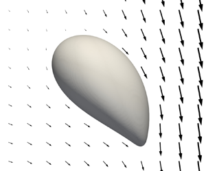



1. Introduction
When a bubble rises with a relative velocity in a shear flow, the surrounding liquid exerts a force on the bubble in a direction perpendicular to its relative motion. This force is commonly known as the shear-induced lift force. Accurate models for the lift force are important to correctly predict the spatial distribution of the bubbles in many bubbly flow applications (Mudde Reference Mudde2005; Ertekin et al. Reference Ertekin, Kavanagh, Fletcher and McClure2021). For example, in bubbly pipe flows, the lift force causes the bubbles to migrate either towards the pipe wall or the pipe centre, depending on the two-phase flow conditions (Lucas, Krepper & Prasser Reference Lucas, Krepper and Prasser2001). This change of the lift force direction also affects the flow stability in bubble columns because the direction influences whether the bubbles spread uniformly or in clusters (Lucas, Prasser & Manera Reference Lucas, Prasser and Manera2005; Mazzitelli & Lohse Reference Mazzitelli and Lohse2009).
Because of its practical importance, research related to discovering fundamental features of the lift force has been going on for more than 60 years. Based on previous studies, we distinguish four mechanisms that govern the net lift force acting on clean bubbles depending on the specific flow conditions. Lighthill (Reference Lighthill1956) described analytically the inviscid and weakly sheared flow past a sphere and showed that the lift force is induced by a pair of counter-rotating vortices in the sphere's wake. Auton (Reference Auton1987) further developed this work and evaluated the lift force acting on the sphere by calculating the effect of the vortices on the velocity field. In low-Reynolds-number shear flows, Saffman (Reference Saffman1965) derived an analytical expression for the lift force acting on a solid sphere. This expression was extended for spherical bubbles by Legendre & Magnaudet (Reference Legendre and Magnaudet1997) and a connection was outlined between the lift force and the vorticity generated at the surface of the bubble. Today, it is well established that for a spherical bubble in laminar shear flows and at any bubble Reynolds number, the lift force is positive (towards the pipe wall in upward pipe flows) (Legendre & Magnaudet Reference Legendre and Magnaudet1998).
However, there are additional distinct physical mechanisms that generate a lift force on non-spherical (and deformable) bubbles in linear shear flows. In particular, at low Reynolds numbers, a deformation-induced lift force acts on non-spherical bubbles in a shear flow (Magnaudet, Takagi & Legendre Reference Magnaudet, Takagi and Legendre2003), and, at higher Reynolds numbers, the vorticity produced at the deformed bubble surface is stretched and tilted into a pair of counter-rotating streamwise vortices with the opposite sign to that for spherical bubbles (Adoua, Legendre & Magnaudet Reference Adoua, Legendre and Magnaudet2009). The governing mechanisms for deformed bubbles generate lift forces that scale differently and act in the opposite direction than the lift forces generated by the governing mechanisms for spherical bubbles. Therefore, under certain conditions, the net lift force may change sign (bubbles migrate towards the pipe centre in upward pipe flows). The sign reversal has been observed in both simulations (Ervin & Tryggvason Reference Ervin and Tryggvason1997; Bothe, Schmidtke & Warnecke Reference Bothe, Schmidtke and Warnecke2006; Adoua et al. Reference Adoua, Legendre and Magnaudet2009; Dijkhuizen, van Sint Annaland & Kuipers Reference Dijkhuizen, van Sint Annaland and Kuipers2010) and experiments (Tomiyama et al. Reference Tomiyama, Tamai, Zun and Hosokawa2002; Aoyama et al. Reference Aoyama, Hayashi, Hosokawa, Lucas and Tomiyama2017; Hessenkemper et al. Reference Hessenkemper, Ziegenhein, Rzehak, Lucas and Tomiyama2021).
The relative importance between the four lift force mechanisms varies with the flow conditions and results in a highly nonlinear behaviour of the net lift force. The nonlinearity makes it very difficult to develop universally applicable lift force models. This difficulty is clearly illustrated by the numerous and rather different lift force correlations proposed in the literature (Pang & Wei Reference Pang and Wei2011).
Although all four mechanisms were identified in previous studies, there is still a lack of a comprehensive explanation for all mechanisms based on the same observable and quantifiable flow features. This deficiency limits a clear understanding of the net lift force behaviour at different flow conditions, makes it difficult to quantify the relative importance of each mechanism and, therefore, hinders the development of more universally applicable lift force models.
Our aim is, therefore, to provide a general description of the flow phenomena behind the four lift force mechanisms based on the same flow features. Specifically, we provide a theoretical framework for the force acting on a bubble in a linear shear flow in terms of moments of the bubble-induced vorticity by extending the previous works of, e.g. Wu (Reference Wu1981), Noca, Shiels & Jeon (Reference Noca, Shiels and Jeon1999) and Biesheuvel & Hagmeijer (Reference Biesheuvel and Hagmeijer2006). Based on these results, we provide formulations that explain the lift forces induced by the different mechanisms. Then, we perform three-dimensional (3-D) multiphase direct numerical simulations (DNS) to support our theoretical framework and illustrate how the lift force mechanisms can be explained in terms of bubble-induced vorticity dynamics. Finally, based on our findings, we qualitatively explain how the different mechanisms cause the nonlinear net lift force behaviour under a wide range of relevant flow conditions.
Our simulations also show how the lift force scales with the shear rate under conditions governed by the different mechanisms. This study extends the current knowledge regarding the role of the shear on the lift force, which is an important aspect to consider when developing improved lift force models.
2. Background
This section provides a brief overview of the state of the art of the lift force acting on clean bubbles in linear shear flows. We begin with presenting the governing parameters of the problem and then introduce and describe the different lift force mechanisms identified in previous works. We continue to discuss how these mechanisms influence the behaviour of the net lift force and then describe how the lift force scales with the shear rate depending on the governing mechanism.
2.1. Governing parameters
The problem of a clean bubble rising in a linear shear flow is described entirely by the following five dimensionless parameters (Tripathi, Sahu & Govindarajan Reference Tripathi, Sahu and Govindarajan2014): the Galilei number  $Ga = {\rho _l \sqrt {gD}D}/{\mu _l}$ that relates buoyancy to viscous forces; the Eötvös number
 $Eo = {\rho _l g D^2}/{\sigma }$ that relates buoyancy to surface tension forces; the dimensionless shear rate
 $Sr = {|\omega _\infty | D}/{\sqrt {gD}}$; the density ratio
 $\rho _r={\rho _l}/{\rho _g}$; and the dynamic viscosity ratio
 ${\mu _r = {\mu _l}/{\mu _g}}$.
We define  $D$ as the spherical equivalent bubble diameter,
 $g$ is the value of gravitational acceleration,
 $\sigma$ is the surface tension,
 $\omega _\infty$ is the shear rate of the surrounding flow and the symbols
 $l$ and
 $g$ indicate the liquid and gas phases, respectively. For all the simulation cases in this paper, we use the density and viscosity ratios of
 $\rho _r = 1000$ and
 $\mu _r = 100$ that represent the most relevant gas–liquid systems.
Sharaf et al. (Reference Sharaf, Premlata, Tripathi, Karri and Sahu2017) investigated the effects of  $\rho _r$ and
 $\mu _r$ on the bubble dynamics in the range
 $\rho _r, \mu _r \in [10,10\,000]$ for a bubble rising in a quiescent liquid with the other governing parameters kept constant. They obtained very similar bubble shapes and rise velocities in the entire investigated ranges but noted a change in the bubble trajectories at the highest density and viscosity ratios. Still, if
 $\rho _r$ and
 $\mu _r$ are of similar orders of magnitude as our ratios, no significant effect of
 $\rho _r$ and
 $\mu _r$ on the bubble dynamics is expected (Loisy, Naso & Spelt Reference Loisy, Naso and Spelt2017). In addition, Bunner & Tryggvason (Reference Bunner and Tryggvason2002) studied the effects of
 $\rho _r$ and
 $\mu _r$ on the bubble dynamics and argued that at ratios above
 $50$, the pressure and viscous forces acting on the bubble interface by the gaseous phase are much smaller than the forces acting on the interface by the liquid phase. Hence, at ratios larger than
 $50$, the effects of the density and viscosity ratios are essentially negligible. By fixing the density and viscosity ratios (well above
 $50$), we have three independent dimensionless parameters (
 $Ga,Eo,Sr$) that essentially govern our problem of a bubble rising in a linear shear flow.
The Galilei (Eötvös) number plays a similar role to the more familiar Reynolds (Weber) number, but is defined with the characteristic rise velocity  $\sqrt {gD}$ due to buoyancy forces rather than the relative velocity between the liquid and the bubble. The Reynolds and Weber numbers are defined as
 $Re = {\rho _l |\overline {\boldsymbol {V}_{rel}}| D}/{\mu _l}$ and
 $We = {\rho _l |\overline {\boldsymbol {V}_{rel}}|^2 D}/{\sigma }$ where
 $|\overline {\boldsymbol {V}_{rel}}|$ is the quasisteady relative velocity of the bubble. Considering that
 $|\overline {\boldsymbol {V}_{rel}}|$ is unknown a priori, the Galilei (Eötvös) number is better suited to describe the problem of a rising bubble than the Reynolds (Weber) number. Nevertheless, by using the Froude number,
 $Fr = Re/Ga = |\overline {\boldsymbol {V}_{rel}}| / \sqrt {gD}$, it is straightforward to map between functions
 $f(Ga) \leftrightarrow f(Re)$,
 $f(Eo) \leftrightarrow f(We)$. Note also that
 $Fr \approx O(1)$ for the bubbles considered in this study.
To facilitate the discussions in this paper, it is useful to define a number of approximate ranges of our governing parameters. Based on the differences in the characteristic behaviour of the bubble dynamics and the lift force, we consider the Galilei number low at  $Ga \leq O(1)$, moderate at
 $Ga = O(10)$ and high at
 $Ga \geq O(100)$. The Eötvös number is deemed low at
 $Eo \leq O(0.1)$, moderate at
 $Eo = O(1)$ and high at
 $Eo \geq O(10)$, while the dimensionless shear rate is regarded low at
 $Sr \leq O(0.001)$, moderate at
 $Sr = O(0.01)$ and high at
 $Sr \geq O(0.1)$.
2.2. Brief overview of previous studies on lift force mechanisms
In this work we focus on four distinct lift force mechanisms that together qualitatively explain the behaviour of the lift force observed in our own simulations and previous numerical and experimental studies.
The first mechanism is denoted the Saffman-mechanism, and it governs the lift force for spherical bubbles (low  $Eo$) at low
 $Ga$ numbers. In principle, the same mechanism governs the lift force acting on a solid sphere in similar conditions. Although viscous effects dominate at low
 $Re$ numbers, Bretherton (Reference Bretherton1962) showed that no transverse force on a single rigid spherical particle could be derived based on creeping flow equations in a unidirectional flow field. This motivated Saffman (Reference Saffman1965) to take small inertia effects into account and thereby successfully derive an analytical solution for the lift force acting on solid spheres at low
 $Re$ numbers in shear flows. Legendre & Magnaudet (Reference Legendre and Magnaudet1997) extended the results of Saffman (Reference Saffman1965) for spherical drops or bubbles at arbitrary viscosity. Physically, the Saffman-mechanism is a result of that the particle induces velocities that are advected asymmetrically by the surrounding shear flow (Legendre & Magnaudet Reference Legendre and Magnaudet1998). Therefore, the resulting velocity and pressure fields induce a force on the particle with a non-zero transverse component. In terms of vorticity, the Saffman-mechanism is a consequence of the vorticity generated at the bubble surface and the asymmetric advection of that vorticity by the surrounding shear flow (Legendre & Magnaudet Reference Legendre and Magnaudet1997, Reference Legendre and Magnaudet1998; Magnaudet & Eames Reference Magnaudet and Eames2000).
For a spherical bubble with a higher  $Ga$ number, the Lighthill- or L-mechanism increasingly dominates over the Saffman-mechanism (the L-mechanism dominates at
 $Re>20$ for spherical bubbles in Legendre & Magnaudet (Reference Legendre and Magnaudet1998)). The L-mechanism arises because the bubble disturbance field stretches and tilts the vorticity in the upstream shear flow into a pair of counter-rotating streamwise vortices in the bubble wake (Lighthill Reference Lighthill1956; Auton Reference Auton1987; Adoua et al. Reference Adoua, Legendre and Magnaudet2009). This pair of vortices induces a liquid motion in the transverse direction that pushes the bubble in the opposite transverse direction due to Newton's third law. Despite the fundamental differences between the Saffman- and L-mechanisms, it is interesting to note that, as pointed out by Legendre & Magnaudet (Reference Legendre and Magnaudet1998), both mechanisms are governed by vorticity and the asymmetric advection due to the shear flow. Both the Saffman- and L-mechanisms dominate the lift force acting on spherical bubbles and induce a positive lift force (towards a higher relative velocity).
For deformed bubbles, two other distinct mechanisms are important to consider. The first one is termed the A-mechanism and is a consequence of the fact that bubbles, at low-to-moderate  $Ga$, and moderate-to-high
 $Eo$, are deformed asymmetrically by the liquid shear flow (Taylor Reference Taylor1932; Ervin & Tryggvason Reference Ervin and Tryggvason1997; Tomiyama et al. Reference Tomiyama, Tamai, Zun and Hosokawa2002; Magnaudet et al. Reference Magnaudet, Takagi and Legendre2003; Zhang, Ni & Magnaudet Reference Zhang, Ni and Magnaudet2021). Ervin & Tryggvason (Reference Ervin and Tryggvason1997) studied such bubbles numerically and showed a relation between the sign of the bubble circulation and the sign of the lift force for two-dimensional (2-D) bubbles rising in a linear shear flow. In these simulations, an almost circular bubble experienced a positive lift force but a negative circulation. In contrast, an asymmetrically deformed bubble experienced a negative lift force but a positive circulation. In the same study, bubble simulations in three dimensions with similar governing parameters showed the same sign of the lift force as their 2-D counterparts. In two dimensions (the
 $xy$-plane), the only non-zero vorticity component is
 $\omega _z$ and the circulation around the bubble interface is
 $\varGamma _B = \int _{A_B} \omega _z \, {\rm d} A$, where
 $A_B$ is the bubble area. These findings also suggest a connection between the bubble-induced
 $\omega _z$ and the induced lift force on bubbles at low
 $Ga$ conditions. By way of analogy, the lift force on a 2-D airfoil in inviscid flows is also a direct consequence of the induced vorticity and the corresponding circulation around the airfoil, according to the well-known Kutta–Joukowski theory (Wu Reference Wu1981; White Reference White2011).
The other mechanism relevant for deformed bubbles is termed the S-mechanism. It governs the lift force in an intermediate range of moderate-to-high  $Ga$ numbers and at sufficiently high bubble deformations (moderate-to-high
 $Eo$) (Adoua et al. Reference Adoua, Legendre and Magnaudet2009). The S-mechanism results from the stretching and tilting of the vorticity generated at the bubble surface into a pair of counter-rotating streamwise vortices in the bubble wake. These vortices have the opposite sign compared with those in the L-mechanism and, therefore, induce a negative lift force. The key difference between the S- and L-mechanisms is that, in the S-mechanism, the streamwise vorticity originates from the vorticity generated at the bubble surface. In contrast, in the L-mechanism, the streamwise vorticity is generated by stretching and tilting of the vorticity in the upstream shear flow.
In summary, the Saffman- and L-mechanisms dominate for spherical bubbles and generate lift forces in the positive direction. Conversely, for deformed bubbles, the A- and S-mechanisms generally dominate and induce lift forces in the negative direction. Figure 1 represents an overview of the governing mechanisms, the direction of the lift force, and the corresponding sign of the lift force coefficient  $C_L$ (defined in (2.1)) in the
 $(Ga, Eo)$-phase plane. In addition, typical bubble shapes and trajectories from our simulations are included to illustrate the effect of the
 $(Ga, Eo)$-parameters and the wide range of bubble dynamics that is obtained. The dashed lines in figure 1 are a schematic representation of the regions where the four lift force mechanisms dominate the net lift force. The location of these lines is loosely based on the previous studies discussed in this section and the available
 $C_L$ data shown in figure 2.
The  $(Ga,Eo)$-phase plot illustrating the different behaviours of the lift force. The dashed lines represent qualitative indications of the regions where the four lift force mechanisms dominate the net lift force acting on a single bubble in a linear shear flow. Typical bubble shapes and trajectories (blue lines behind the bubbles) are shown for the case where the liquid velocity relative to the bubble is higher on the right-hand side of the bubble (representation of the relative velocity field above the plot). The bubble positions in the phase plot indicate the parameters used in their respective simulations. The bubble trajectories are scaled to more clearly show the direction of the lateral motion. Note also that in some regions,
 $Sr$ influences what mechanism dominates the net lift force and this dependence is investigated in § 6.5.

The  $(Ga,Eo)$-phase plot with
 $C_L$ data (dots) obtained from available experimental and numerical data on freely deforming bubbles in linear shear flows with moderate-to-high
 $Sr$. The contours illustrate the
 $C_{L,fit}$-surface obtained by fitting (2.2) to these points and the soft constraint
 $C_{L,fit} = 0.5$ at high
 $Ga$ and low
 $Eo$ since theoretically
 $C_L=0.5$ for a spherical bubble in a weakly sheared inviscid flow (Auton Reference Auton1987). The colour scale of the data points and contours is limited to the range
 $[-1,1]$ for visualization purposes. The dashed black line indicates the contour line
 $C_{L,fit} = 0$. The large variation of
 $C_L$ at high
 $Eo$ or low
 $Ga$ illustrates the change of scaling of the lift force in regions of the phase-space governed by the different lift force mechanisms.

Based on the above brief overview of the four lift force mechanisms, it is interesting to note that although they have distinct physical explanations, they can all be interpreted in terms of the bubble-induced vorticity. Therefore, in this work, we focus on how bubble-induced vorticity can explain all four mechanisms. First, it is, however, appropriate to discuss how the four lift force mechanisms and the governing parameters  $(Ga,Eo,Sr)$ influence the net lift force acting on the bubble.
2.3. Behaviour of the net lift force
The same functional form of the lift force is typically assumed for all values of the governing parameters. Nevertheless, depending on the governing parameters, the lift force is induced by different physical mechanisms that, in general, do not scale similarly. The most common functional form is appropriate for the lift force acting on a spherical bubble at high  $Ga$ and weakly sheared flows (where the L-mechanism dominates) and is given by (un Reference Ẑun1980; Auton Reference Auton1987; Drew & Lahey Reference Drew and Lahey1987)
 \begin{equation} \boldsymbol{F_L} ={-}C_L \varOmega_g \rho_l \boldsymbol{V}_{rel} \times \boldsymbol{\omega}_U ,\end{equation}
where  $C_L$ is the lift force coefficient,
 $\varOmega _g$ is the bubble volume,
 $\rho _l$ is the liquid density,
 $\boldsymbol {V}_{rel} = \boldsymbol {V - U}$ is the relative velocity between the bubble (
 $\boldsymbol {V}$) and the undisturbed liquid (
 $\boldsymbol {U}$) evaluated at the bubble position and
 $\boldsymbol {\omega }_U = \boldsymbol {\nabla } \times \boldsymbol {U}$ is the undisturbed liquid vorticity evaluated at the bubble position.
Although, in principle,  $C_L=f(Ga,Eo,Sr)$, the functional form of (2.1) is still suitable for slightly deformed bubbles at low-to-moderate
 $Eo$, and moderate-to-high
 $Ga$ numbers (where the L-mechanism still dominates). This is illustrated in figure 2 where the
 $C_L$-contours show relatively small variations within the ranges of, say,
 $Eo<1$ and
 $Ga>10$.
The  $C_L$-contours in figure 2 are computed by fitting a surface (defined by (2.2)) to the available experimental and numerical data (dots in figure 2) on freely deforming bubbles in shear flows obtained in Dijkhuizen et al. (Reference Dijkhuizen, van Sint Annaland and Kuipers2010), Aoyama et al. (Reference Aoyama, Hayashi, Hosokawa, Lucas and Tomiyama2017), Feng & Bolotnov (Reference Feng and Bolotnov2017), Ziegenhein, Tomiyama & Lucas (Reference Ziegenhein, Tomiyama and Lucas2018) and Hessenkemper et al. (Reference Hessenkemper, Ziegenhein, Rzehak, Lucas and Tomiyama2021) at moderate-to-high
 $Sr$. The fitted surface is described by the ratio of two third-order surfaces
 \begin{equation} C_{L,fit} = \frac{ -\frac{9}{10}x^3 - \frac{97}{10}x^2y + \frac{79}{10}x^2 - 7xy^2 + 10xy - \frac{49}{10}x - \frac{21}{5}y^3 - \frac{19}{5}y + \frac{18}{5}y^2 + 1} { x^3 - \frac{23}{5}x^2y + \frac{51}{10}x^2 + \frac{21}{5}xy^2 - \frac{41}{10}xy + \frac{87}{10}x - 3y^3 + \frac{31}{5}y - \frac{1}{2}y^2 - 4} , \end{equation}
where  $x=\log _{10}(Ga)$ and
 $y=\log _{10}(Eo)$. Despite some scatter in the available data, the absolute standard deviation is
 $0.09$ between the fitted surface and the data points. At high
 $Ga$ and low
 $Eo$, the
 $C_{L,fit}$-surface approaches the analytical solution of
 $C_{L,s,\infty } = 0.5$ (Auton Reference Auton1987) for a spherical bubble in a weakly sheared inviscid flow. At around
 $Ga < 3$ and far from known data points the expression (2.2) is not suitable.
For approximately spherical bubbles (low  $Eo$ numbers),
 $C_L$ is always positive but increases rapidly at low
 $Ga$ numbers where the Saffman-mechanism dominates (Legendre & Magnaudet Reference Legendre and Magnaudet1998). The increase of
 $C_L$ at low
 $Ga$ clearly demonstrates that the lift force scales differently when the Saffman-mechanism dominates.
A different lift force scaling is also displayed for more deformed bubbles (moderate-to-high  $Eo$), where
 $C_L$ varies significantly to account for the forces induced by the A- and S-mechanisms. Because of the two latter mechanisms,
 $C_L$ decreases and reaches negative values for sufficiently high
 $Eo$ (a sign reversal of
 $C_L$ occurs roughly in the range
 $2< Eo<4$ for all
 $Ga$ considered in figure 2).
In summary, the behaviour of the net lift force clearly varies with the governing parameters  $(Ga,Eo)$, and we aim in this paper to provide a comprehensive explanation for these variations. In addition, we should also introduce how the third governing parameter, the non-dimensional shear rate
 $Sr$, influences the net lift force.
2.3.1. Influence of the shear rate on the lift force
The formulation of (2.1) assumes that the lift force scales linearly with the shear rate. Still, when the L-mechanism is not dominant, the scaling with the shear rate can be highly nonlinear. Thus,  $C_L$ in (2.1) takes into account also the nonlinear scaling with the shear rate, so that
 $C_L = f(Ga,Eo,Sr)$.
Several studies have investigated the effect of  $Sr$ on
 $C_L$ with conclusions varying depending on the phase-space region (
 $Ga,Eo,Sr$) under investigation. In very viscous flows (low
 $Ga$), Legendre & Magnaudet (Reference Legendre and Magnaudet1997) extended the theoretical lift force predictions of Saffman (Reference Saffman1965) and McLaughlin (Reference McLaughlin1991) to spherical drops of arbitrary viscosity. For a spherical bubble in very viscous flows, the lift coefficient defined in (2.1) becomes (Legendre & Magnaudet Reference Legendre and Magnaudet1998)
 \begin{equation} C_{L,Saffman} = \frac{6}{{\rm \pi}^2}(Re Sr_{V})^{{-}1/2}J(\epsilon),\end{equation}
where  $Sr_{V} = {|\omega _\infty |D}/{|\overline {\boldsymbol {V}_{rel}}|}$,
 $\epsilon =(Sr_{V}/Re)^{1/2}$ and
 $J(\epsilon )$ is the value of a 3-D integral numerically evaluated by McLaughlin (Reference McLaughlin1991). According to (2.3),
 $C_L$ is clearly a complex function of both
 $Re$ (or
 $Ga$) and
 $Sr$ in the low
 $Ga$ and low
 $Eo$ regime.
Legendre & Magnaudet (Reference Legendre and Magnaudet1998) investigated numerically the lift force acting on fixed spherical bubbles in linear shear flows. They found that  $C_L$ increased as
 $Re$ decreased for
 $Re<5$ and that
 $C_L$ was significantly dependent on
 $Sr$ at
 $Re<5$. The increase of
 $C_L$ at low
 $Ga$ can qualitatively be observed in figure 2 in the region
 $Ga<10, Eo<1$. In addition, for spherical bubbles at moderate-to-high
 $Ga$ where the L-mechanism dominates, Legendre & Magnaudet (Reference Legendre and Magnaudet1998) showed that
 $C_L$ was nearly independent of
 $Sr$ and that
 $C_L$ tended asymptotically towards the analytical prediction of
 $C_{L,s,\infty }=0.5$ as
 $Ga \to \infty$.
In the experimental work of Tomiyama et al. (Reference Tomiyama, Tamai, Zun and Hosokawa2002),  $C_L$ was studied in the approximate ranges (
 $6< Ga<88$), (
 $1.4< Eo<5.7$) and (
 $Sr<0.2$). Within these parameter ranges, the authors did not observe any significant effect of
 $Sr$ on
 $C_L$.
Dijkhuizen et al. (Reference Dijkhuizen, van Sint Annaland and Kuipers2010) used a front-tracking DNS technique to study  $C_L$ in the parameter ranges of approximately (
 $4< Ga<1640$), (
 $0.1< Eo<11$) and (
 $Sr<0.1$). The authors concluded that
 $Sr$ had no significant effect on
 $C_L$. However, we will show that within the same ranges of
 $Ga$ and
 $Eo$, but using other values of
 $Sr$, the shear rate can significantly alter the value of
 $C_L$ and even change its sign.
The change of sign in  $C_L$ due to variations of
 $Sr$ was also studied numerically by Adoua et al. (Reference Adoua, Legendre and Magnaudet2009) that examined the lift force acting on fixed bubbles of prescribed oblate spheroidal shapes in weakly viscous linear shear flows. Their parameter ranges were (
 $50\leq Re_b \leq 4000$), (
 $0 \leq Sr_b \leq 0.2$) and (
 $1.0 \leq \chi \leq 2.7$), where
 $Re_b = 2 b U_0 / \nu$ and
 $Sr_b = 2 \omega _\infty b / U_0$ are defined using the major semiaxis
 $b$ of the bubble, the prescribed relative velocity
 $U_0$, the liquid kinematic viscosity
 $\nu$ and
 $\chi = b/a$ is the ratio of the major to minor semiaxes of the bubble.
In the work of Adoua et al. (Reference Adoua, Legendre and Magnaudet2009), the change of sign of  $C_L$ due to
 $Sr$ is explained by the different scaling of the lift forces induced by the S- and L-mechanisms. Their results suggest that the S-mechanism induces a negative lift force that is almost invariant with
 $Sr$ (at least at low
 $Sr$). In contrast, the L-mechanism induces a positive lift force proportional to
 $Sr$. Consequently, it is argued that the L-mechanism will always dominate the S-mechanism provided
 $Sr$ is large enough.
Thus, given a negative lift force at low  $Sr$, the lift force will change sign at a sufficiently high
 $Sr$ value. However, the use of fixed oblate spheroidal bubbles in the simulations of Adoua et al. (Reference Adoua, Legendre and Magnaudet2009) limits the conditions at which the results are relevant to situations where
 $Re= O(100$–
 $1000)$,
 $We=O(1)$ and
 $Sr \ll 1$. Therefore, it is unclear if the L-mechanism will always dominate at high enough
 $Sr$ also for freely deformable and moving bubbles outside these parameter ranges.
Clearly, the dominating lift force mechanisms vary depending on the considered phase-space region ( $Ga$,
 $Eo$,
 $Sr$). As indicated by the above brief review, our understanding of the behaviour of the lift force and how it is influenced by
 $Sr$ is limited to specific regions of the phase-space. Therefore, one of the aims of this paper is to shed light on how the lift force scales with the shear rate under conditions where the different lift force mechanisms dominate.
3. Problem statement
In this paper we aim at providing a comprehensive explanation of the four lift force mechanisms that induce the lift force acting on a bubble rising in a linear shear flow. We also aim at determining how the lift force scales with the undisturbed shear rate in cases governed by the different lift force mechanisms.
Specifically, we study freely moving and deformable bubbles rising in an infinite linear shear flow. Gravity acts in the negative  $y$-direction and induces a buoyancy force on the bubble that acts in the positive
 $y$-direction. We consider the case of an undisturbed liquid linear shear flow
 $\boldsymbol {U} = (0, x\, {\rm d} U_y/{{\rm d} x}, 0)$ with the shear rate
 $\omega _\infty = {\rm d} U_y/{{\rm d} x} < 0$ so that the undisturbed liquid velocity relative to the bubble is higher on the bubble side towards the positive
 $x$-direction. Figure 3 shows a schematic view of this problem. According to (2.1), this set-up gives a lift force coefficient
 $C_L$ that is positive if the lift force acts in the positive
 $x$-direction and a negative
 $C_L$ if the lift force acts in the negative
 $x$-direction.
Schematic view of the problem. A freely moving and deformable bubble rises due to buoyancy in an infinite linear shear flow where gravity acts in the negative  $y$-direction. We consider an undisturbed shear flow with
 ${\rm d} U_y/{{\rm d} x} < 0$ so that for a positive (negative)
 $C_L$ the bubble moves in the positive (negative)
 $x$-direction. The coordinate systems illustrate the non-inertial MRF and the laboratory reference frame. The velocity field
 $\hat {\boldsymbol {u}}$ is the velocity relative to the MRF, and the MRF follows the bubble in the laboratory reference frame (i.e.
 $\boldsymbol {V}_{mrf}=\boldsymbol {V}$).

We provide a theoretical framework that relates the lift force acting on the bubble to moments of bubble-induced vorticity. In addition, we support the theoretical framework by performing fully resolved 3-D multiphase DNS simulations of freely moving and deformable bubbles in a linear shear flow. These simulations confirm the validity of the theoretical framework and demonstrate the specific vorticity dynamics associated with the four lift force mechanisms.
Then, we examine with our simulations how  $C_L$ scales with
 $Sr$ under conditions where the different lift force mechanisms dominate. This investigation indicates the regions of the phase-space (
 $Ga$,
 $Eo$,
 $Sr$) where
 $C_L$ is independent of
 $Sr$ (the lift force scales linearly with the shear rate) and the regions where the
 $C_L$ coefficient needs to account for any nonlinear scaling.
Within the shear-rate study, we extend the work of Adoua et al. (Reference Adoua, Legendre and Magnaudet2009) to freely moving and deformable bubbles. Particularly, we study whether their findings that the L-mechanism always dominates the S-mechanism at high enough shear rates also hold for freely moving and deformable bubbles (at high  $Ga$ and
 $Eo > 1$), where the lateral bubble motion and asymmetric bubble deformations may influence the net lift force behaviour.
3.1. Considerations in the present investigation
In general, a rising bubble can experience transient lift forces even without the presence of shear in the surrounding liquid flow (Magnaudet & Mougin Reference Magnaudet and Mougin2007; Ern et al. Reference Ern, Risso, Fabre and Magnaudet2012). Such lift forces give rise to unsteady bubble trajectories that display a fascinating range of behaviours, some of which develop over relatively long spatiotemporal scales. For example, Cano-Lozano et al. (Reference Cano-Lozano, Martinez-Bazan, Magnaudet and Tchoufag2016) and Tripathi, Sahu & Govindarajan (Reference Tripathi, Sahu and Govindarajan2015) used DNS to study single bubbles rising in a quiescent liquid and obtained rectilinear, zigzagging, spiralling and even chaotic bubble trajectories depending on the governing parameters.
In the non-rectilinear trajectories, the bubble experiences a fluctuating lift force corresponding to the unsteady lateral motion. By averaging this lift force over a sufficient number of oscillations, we obtain a quasisteady lift force. The latter force is generally non-zero with the shear present in the undisturbed liquid flow and zero without the presence of shear. We focus in this work on the behaviour of this quasisteady lift force acting on freely moving and deformable bubbles in a linear shear flow.
We assume that no phase change occurs. Furthermore, possible non-ideal effects on the lift force, such as the presence of walls, free stream turbulence and the presence of other bubbles, are not considered. In the presence of surfactants, the contaminated bubble interface may become less mobile, the surface tension modified and the bubble shape therefore altered. Surfactants, therefore, change the surface vorticity generation and bubble dynamics and thus influence the lift force acting on the bubble (Hayashi & Tomiyama Reference Hayashi and Tomiyama2018). Surfactants would therefore modify the regions of the phase-space where the different lift force mechanisms dominate the net lift force, although the fundamental flow phenomena of each mechanism should be the same. Even though all non-ideal flow conditions certainly influence the bubble dynamics (Bunner & Tryggvason Reference Bunner and Tryggvason2003; Lu & Tryggvason Reference Lu and Tryggvason2008), we believe it is essential first to understand the behaviour of the lift force in the simplest case of a single isolated clean bubble in linear shear flows. For this reason, we consider the lift forces on clean, freely moving and deformable (realistically shaped) bubbles.
4. Numerical framework
Although presenting the theoretical framework before the numerical framework may seem logical, we choose to do it here in the opposite order. The reason is that we want to introduce in this section a moving reference frame (MRF) technique, which is a crucial part of the numerical framework but also of great relevance in the theoretical part of our analysis.
The different lift force mechanisms have undoubtedly a complex interaction and thus need to be considered together. Also, since the mechanisms interact with the bubble shape and motion, it is essential to capture the latter features realistically. For these reasons, we use a multiphase DNS framework based on the volume of fluid approach. In this framework, we use a MRF technique to facilitate tracking of the bubbles for sufficiently long periods to obtain quasisteady quantities. The numerical framework is outlined in this section, but a detailed description and validation can be found in Hidman et al. (Reference Hidman, Ström, Sasic and Sardina2022).
We start by non-dimensionalizing all relevant variables by scaling with the diameter  $D$, gravitational acceleration
 $g$, the surrounding liquid density
 $\rho _l$ and the liquid viscosity
 $\mu _l$. The non-dimensional variables are the spatial coordinates
 $x^*_i = x_i/D$, velocity
 $u^*_i = u_i / \sqrt {gD}$, time
 $t^*= t/\sqrt {D/g}$, density
 $\rho ^* = \rho /\rho _l$, dynamic viscosity
 $\mu ^* = \mu /\mu _l$, pressure
 $p^* = p/(\rho _l g D)$, gravitational acceleration
 $g_i^* = g_i/g$ and the bubble interface curvature
 $\kappa ^* = \kappa D$. Unless otherwise stated, all variables in the remainder of this paper are non-dimensionalized accordingly and the asterisk notation is henceforth omitted.
In this work we study the quasisteady dynamics of a bubble rising in a linear shear flow. For this problem, it is not trivial to a priori select the required size of the computational domain since the bubble dynamics may develop over relatively large spatial scales. Because of the large density ratio coupled with the gravitational force, the bubble rises at a high velocity and may travel long vertical distances. Also, at high liquid shear, the bubble can be both advected large vertical distances by the high-velocity shear flow and, due to the lift force, reach the horizontal boundaries of the domain. In addition, the lift force has been shown to be sensitive to boundary effects, and thus a sufficient distance between the bubble and the domain boundaries needs to be maintained. To solve these challenges, we use a MRF technique that allows the computational domain to follow the motion of a bubble and to keep the bubble at its initial position within this domain.
We change the frame of reference from a laboratory, or absolute, reference frame to a non-inertial reference frame moving with the bubble by making the following change of variables:
 $$\begin{gather} \hat{t} = t , \end{gather}$$
 $$\begin{gather}\hat{x}_i = x_i - x_{mrf,i} , \end{gather}$$
 $$\begin{gather}\hat{u}_i = u_i - V_{mrf,i} , \end{gather}$$
where  $\hat {x}_i$ and
 $\hat {u}_i$ are the non-dimensional position and velocity within the MRF, and
 $x_{mrf,i}$ and
 $V_{mrf,i}$ are the absolute position and velocity of the MRF itself. An illustration of these reference frames is shown in figure 3. Here,
 $\hat {\boldsymbol {r}}_B$ represents the bubble centre of mass in the MRF, the gravity acts in the negative
 $y$-direction, and the surrounding liquid shear flow field is given by
 $U_y = -Sr x$.
The non-dimensional governing equations for the two-phase flow in the non-inertial MRF are
 $$\begin{gather} \frac{\partial \hat{u}_i}{\partial \hat{x}_i} = 0, \end{gather}$$
 $$\begin{gather}\rho\left(\frac{\partial \hat{u}_i}{\partial \hat{t}} + \hat{u}_j\frac{\partial \hat{u}_i}{\partial \hat{x}_j} \right) = \rho\left (g_i - a_{mrf,i}\right) - \frac{\partial p}{\partial \hat{x}_i} + \frac{1}{Ga}\frac{\partial}{\partial \hat{x}_j}\left(\mu\left(\frac{\partial \hat{u}_i}{\partial \hat{x}_j}+\frac{\partial \hat{u}_j}{\partial \hat{x}_i}\right)\right) + \frac{\hat{\kappa}\delta_S \widehat{n_i}}{Eo}, \end{gather}$$
 $$\begin{gather}\frac{\partial c}{\partial \hat{t}} + \frac{\partial c \hat{u}_i}{\partial \hat{x}_i} = 0, \end{gather}$$
where  $a_{mrf,i}$ represents the acceleration of the MRF,
 $\delta _S$ is the Dirac distribution function that localizes the surface tension term at the interface and
 $c$ is the volume fraction field. The density
 $\rho$ and viscosity
 $\mu$ are computed using
 $$\begin{gather} \rho(c) = c + (1-c)/\rho_r, \end{gather}$$
 $$\begin{gather}\mu(c) = (c + (1-c)\mu_r )^{{-}1}, \end{gather}$$
where the symbols  $l$ and
 $g$ indicate the liquid and gas phases. The viscosity is defined with a harmonic mean that is generally more accurate at the gas–liquid interfaces with a continuous shear stress that we consider in this work (Tryggvason, Scardovelli & Zaleski Reference Tryggvason, Scardovelli and Zaleski2011). The MRF should follow the bubble trajectory and keep the bubble at its initial relative position within the MRF. We achieve this by continuously updating the acceleration of the MRF using a proportional integral derivative (PID)-controller that minimizes the distance between the bubble centre of mass and its initial position. This approach keeps the velocity of the MRF approximately equal to the bubble absolute velocity
 $V_{mrf,i} \approx V_i$. The entire approach is described in detail in Hidman et al. (Reference Hidman, Ström, Sasic and Sardina2022). We also provide a validation case in Appendix B to confirm that the MRF technique predicts the same bubble dynamics as when using an absolute reference frame and that the predicted lift force agrees with available experimental and numerical studies. Additional comparisons of the predicted lift force using the MRF technique to previous studies are also presented in § 6.5.
The governing equations are solved using the open-source code Basilisk (Popinet Reference Popinet2015) (see basilisk.fr) that has been used extensively for DNS of bubbly flows, see for example Innocenti et al. (Reference Innocenti, Jaccod, Popinet and Chibbaro2021) and Zhang et al. (Reference Zhang, Ni and Magnaudet2021). This code features a cell-centred Cartesian and a tree-structured grid with an efficient adaptive refinement technique that allows us to perform high-resolution 3-D simulations at a feasible computational cost. The surface tension term in (4.5) is implemented with a well-balanced discretization, and the curvature is computed using an accurate height-function method (Popinet Reference Popinet2018).
The system of partial differential equations is solved using a time-splitting projection method, where standard, second-order, numerical schemes are used for the spatial gradients, and the velocity advection term is discretized with the Bell–Colella–Glaz second-order unsplit upwind scheme (Popinet Reference Popinet2003). Here, the pressure and velocity components are solved using a Helmholtz–Poisson-type equation, and the pressure correction is solved as a Poisson problem. For these problems, an efficient multilevel solver is used on the tree-structured grid. The scalar and velocity fields are discretized in time using a staggered second-order method where the velocity is determined at time  $n+1$ and the scalar fields at
 $n+1/2$. To maintain a sharp interface, the piecewise-linear interface reconstruction method is used to reconstruct the volume fraction field as a line in two dimensions or a plane in three dimensions in each computational cell containing the interface (Scardovelli & Zaleski Reference Scardovelli and Zaleski1999). Then, the volume fraction field is advected using a geometric flux estimation based on the reconstructed interface. This procedure ensures a volume fraction field with a minimal amount of smearing at the interface.
4.1. Computational domain, grid and time step settings
There are several numerical challenges to consider when using the framework outlined above. First, the lift force is very sensitive to boundary effects at low  $Ga$ and low
 $Sr$. Theoretical predictions suggest that the inertia and viscous effects induced by the bubble motion are comparable at a distance
 $D_S = O((GaSr)^{-1/2})$ (Legendre & Magnaudet Reference Legendre and Magnaudet1998). To minimize possible boundary effects, we select the domain size so that the distance
 $D_\varGamma$ between the bubble and a domain boundary is always
 $D_\varGamma \geq 10 D_S$. Because of the MRF technique, which keeps the bubble at its initial position in the domain, it is thus sufficient to ensure that the bubble initial position fulfils this requirement. To predict the correct bubble dynamics, the domain must also capture the part of the bubble wake that significantly influences the bubble motion. For this reason, we generally use a domain size of approximately
 $(40D)^3$ (see Appendix A for the specific cases), where the bubble is placed in the centre of the domain and at
 $2/3$ of the vertical height. This set-up captures the bubble wake almost
 $27D$ behind the bubble, similarly to the wake refinement region in Cano-Lozano et al. (Reference Cano-Lozano, Martinez-Bazan, Magnaudet and Tchoufag2016) that studied rising bubbles in a wide range of the governing parameters.
The boundary conditions of the computational domain are defined in table 1 where a hydrostatic pressure field is imposed. The lateral boundaries have either inlet or outlet boundary conditions depending on the normal boundary velocity direction according to  $\hat {\boldsymbol {u}}_{BC}(\hat {\boldsymbol {x}},t) = \boldsymbol {U}(\hat {\boldsymbol {x}},t) - \boldsymbol {V}_{mrf}(t)$.
Boundary conditions for the computational domain. Here,  $n$ denotes the normal direction and
 $t$ the tangential directions of the specific boundary. The lateral boundaries are specified as either inlet or outlet, depending on the direction of the normal boundary velocity.

Since the forces acting on the bubble are intimately connected with the vorticity generated at the bubble surface, we need to take special care to adequately resolve the viscous boundary layers surrounding the bubble. The thickness of the boundary layer is approximately  $O(D/(2Ga^{1/2}))$ (Adoua et al. Reference Adoua, Legendre and Magnaudet2009) and at least four grid points should be placed within the boundary layer to resolve it sufficiently (Legendre & Magnaudet Reference Legendre and Magnaudet1998; Adoua et al. Reference Adoua, Legendre and Magnaudet2009; Kusuno & Sanada Reference Kusuno and Sanada2021). Grid independence studies and validation cases have been performed using this grid resolution criterion with satisfactory results for all the tested cases. In Appendix C, we present a grid convergence study for the case with the highest
 $Ga$, and
 $Eo$-number, studied in this work, and in Appendix A we specify the maximum grid resolution for each simulation case.
We use the adaptive grid refinement technique in Basilisk, where two criteria are used to determine where and to what extent the grid is refined. These criteria are based on a wavelet decomposition method of the volume fraction and velocity fields (Van Hooft et al. Reference Van Hooft, Popinet, Van Heerwaarden, Van der Linden, de Roode and Van de Wiel2018) and provide grid refinements in the regions where the second spatial derivatives of the fields are high. For the velocity field, this method ensures refinement in the viscous boundary layers and bubble wakes, and for the volume fraction field, the refinement method gives an accurate resolution of the bubble interface. The grid is either refined or coarsened based on absolute thresholds for the error allowed in both fields. These thresholds are chosen as  $\epsilon _f = 0.01$ for the volume fraction field and
 $\epsilon _u = 0.003$ for the velocity field and have been verified to give grid-independent results in bubbly flows (Innocenti et al. Reference Innocenti, Jaccod, Popinet and Chibbaro2021).
The time step size is variable and determined using the common Courant–Friedrichs–Lewy criterion (with a Courant number of 0.5), and, since we are dealing with deformable interfaces and surface tension forces, we also consider the time step constraint due to capillary waves. The non-dimensional capillary constraint is  ${\rm \Delta} t \leq \sqrt {{({\rm \Delta} x)^3 Eo}/{2{\rm \pi} }}$, where
 ${\rm \Delta} x$ is the cell size used at the interface (Denner & van Wachem Reference Denner and van Wachem2015). This is typically the limiting constraint in our simulation cases and is hence prohibiting the use of very low
 $Eo$ numbers.
4.2. Evaluating the lift force coefficient  $C_L$

We determine the lift force coefficient by evaluating the time-averaged forces at a quasisteady bubble motion. Using this approach, the time-averaged momentum exchange between the phases is correct (Dijkhuizen et al. Reference Dijkhuizen, van Sint Annaland and Kuipers2010). In non-dimensional form, the time-averaged equation of motion is defined as
 \begin{equation} \left(\frac{1}{\rho_r} + \bar{C}_{AM} \right)\overline{\frac{{\rm d}\boldsymbol{V}}{{\rm d}t}} ={-}\frac{3}{4} \bar{C}_D\overline{|\boldsymbol{V}_{rel}|\boldsymbol{V}_{rel}} - \bar{C}_L\overline{\boldsymbol{V}_{rel}} \times \boldsymbol{\omega}_U + \left(1 - \frac{1}{\rho_r}\right)\boldsymbol{g},\end{equation}
where the overline represents time-averaged quantities, a weak correlation is assumed between the force coefficients and the flow parameters, and the respective terms are the inertia, drag, lift and buoyancy force. Effects due to the Basset force are neglected. At a quasisteady relative velocity  $\overline {{\rm d}\boldsymbol {V_{rel}}/{{\rm d}t}}=0$, the bubble absolute velocity becomes
 \begin{equation} \overline{\frac{{\rm d} \boldsymbol{V}}{{\rm d} t}} = \overline{\frac{{\rm d} \boldsymbol{V}_{rel}}{{\rm d} t}} + \overline{\frac{{\rm d} \boldsymbol{U}(\boldsymbol{r}_B)}{{\rm d} t}} = \overline{(\boldsymbol{V} \boldsymbol{\cdot} \boldsymbol{\nabla})\boldsymbol{U}}. \end{equation}
We assume  $\rho _r \gg 1$, note that
 $\overline {V_x} = \overline {V_{rel,x}}$ and define the steady undisturbed vorticity field
 $\boldsymbol {\omega }_U = (0,0,-Sr)$ in the linear shear flow (where we use
 $\omega _\infty <0$). By solving for
 $\bar {C}_D$ in the
 $y$-direction of (4.9) and substituting the result into the
 $x$-direction of (4.9) we obtain an expression for the lift force coefficient as
 \begin{equation} \bar{C}_L = \frac{\overline{|\boldsymbol{V}_{rel}| V_{rel,x}}}{(\overline{V_{rel,x}})(\overline{|\boldsymbol{V}_{rel}| V_{rel,x}}) + (\overline{V_{rel,y}})(\overline{|\boldsymbol{V}_{rel}| V_{rel,y}})}\left( \frac{1}{Sr} + \bar{C}_{AM} \overline{V_{rel,x}} \right). \end{equation}
In the cases with oscillating trajectories, we compute the time-averaged  $C_L$ from (4.11) over typically 5–10 oscillation periods, excluding the initial transient before reaching a quasisteady motion. In the remainder of the paper we omit the overline notation of
 $C_L$ for brevity. The added mass coefficient depends on the shape of the bubble and is approximated by the linearized relation of Klaseboer et al. (Reference Klaseboer, Chevaillier, Maté, Masbernat and Gourdon2001) and Kusuno & Sanada (Reference Kusuno and Sanada2021):
 $C_{AM} = 0.62\chi -0 .12$. The absolute difference in the
 $C_L$-values using this relation and the value of
 $C_{AM}=0.5$, valid for spherical bubbles, is less than
 $0.01$ for all cases in this study since typically the relative velocity in
 $x$-direction is small and
 $1/Sr \gg \bar {C}_{AM}\overline {V_{rel,x}}$. Equation (4.11) is similar to the expressions used by Bothe et al. (Reference Bothe, Schmidtke and Warnecke2006), Dijkhuizen et al. (Reference Dijkhuizen, van Sint Annaland and Kuipers2010), Aoyama et al. (Reference Aoyama, Hayashi, Hosokawa, Lucas and Tomiyama2017) and Ziegenhein et al. (Reference Ziegenhein, Tomiyama and Lucas2018) to determine
 $C_L$ in both experimental and numerical studies. We also confirm that evaluating (4.11) in our numerical framework predicts
 $C_L$ in agreement with the results of Legendre & Magnaudet (Reference Legendre and Magnaudet1998), where
 $C_L$ was determined by evaluating a stress-integral on the fixed spherical bubble surface. We simulate the case
 $(Ga=50, Eo=0.1, Sr=0.05)$ and obtain
 $C_L=0.46$ using (4.11) with
 $Re=93$ and
 $\chi =1.04$ at a steady state. This is very close to the
 $C_L=0.451$ reported for the corresponding case in Legendre & Magnaudet (Reference Legendre and Magnaudet1998) and their Table 5.
5. Theoretical framework
This section provides a theoretical framework to explain the underlying mechanisms behind the lift force acting on a bubble in a linear shear flow. Because of the connection with the vorticity dynamics, outlined in § 2.2, it seems appropriate to seek an explanation for all four distinct lift force mechanisms in terms of vorticity rather than velocity. By considering the vorticity field, it proves to be possible and useful to divide the flow field into regions where the vorticity is either significant or approximately zero.
For this analysis, we consider the vorticity dynamics in a control volume moving with the bubble and, specifically, the rate of change of the bubble-induced vorticity moments. This approach provides relation (5.1) (derived in Appendix D) for the total force acting on the bubble due to the bubble-induced vorticity. Based on relation (5.1), we examine in § 5.2 the vorticity dynamics that induce transverse forces on the bubble and provide, in § 5.3 and § 5.4, relations that explain the lift forces induced by the different lift force mechanisms. The predictions of the formulae are then supported by numerical demonstration cases presented in §§ 6.1–6.4.
5.1. Relation between total force and bubble-induced vorticity in linear shear flow
The total force  $\boldsymbol {D}$ acting on the bubble in a linear shear flow due to the bubble-induced vorticity
 $\boldsymbol {\tilde {\omega }}$ in a reference frame
 $\hat {\boldsymbol {x}}$, moving with the bubble, is defined as
 \begin{equation} \boldsymbol{D} ={-} \frac{{\rm d} }{{\rm d} t} \left( \frac{1}{2}\rho_l \int_{\varOmega_l+\varOmega_g} \hat{\boldsymbol{x}} \times \boldsymbol{\tilde{\omega}} \, {\rm d} \varOmega \right) + \rho_l \varOmega_g \frac{{\rm d} \boldsymbol{V}_{rel}}{{\rm d} t} , \end{equation}
where  $\varOmega _l$ is the liquid volume encompassing all bubble-induced vorticity,
 $\varOmega _g$ is the volume occupied by the bubble and
 $\boldsymbol {V}_{rel} = \boldsymbol {V} - \boldsymbol {U}(\boldsymbol {r}_B)$ is the relative velocity between the bubble and the undisturbed liquid. A detailed derivation of (5.1) is given in Appendix D. The relation (5.1) is a reformulation of the relation between the vorticity moments and forces acting on bodies in viscous flows, presented in for example Wu (Reference Wu1981), Noca et al. (Reference Noca, Shiels and Jeon1999) and Biesheuvel & Hagmeijer (Reference Biesheuvel and Hagmeijer2006), into a MRF and in the presence of a surrounding shear flow. We have also validated in Appendix E that (5.1) evaluated in our numerical framework predicts drag forces on both fixed spheres and rising bubbles in agreement with well-known correlations. Based on (5.1), we analyse the vorticity moments that may induce transverse forces on the bubble in the coming sections.
5.2. Relation between the transverse force and bubble-induced vorticity in linear shear flow
We aim to provide a qualitative explanation for the lift force induced by the bubble-induced vorticity dynamics. For this purpose, we use a methodology similar to that which Wu (Reference Wu1981) used to determine the forces acting on a body in viscous flows.
Consider the bubble rising in a linear shear flow illustrated in figure 4. Gravity acts in the negative  $y$-direction and induces a buoyancy force that makes the bubble rise in the positive
 $y$-direction. The liquid volume
 $\varOmega _l$ surrounds the bubble and the entire disturbance field generated by the bubble motion. Two subregions that follow the motion of the bubble are defined within
 $\varOmega _l$; the MRF-region with a constant volume
 $\varOmega _{mrf}$ and the wake-region
 $\varOmega _{wake}$, where the volume increases as the bubble rises and the wake grows longer. The velocity field within these moving regions is described by
 $\hat {\boldsymbol {u}}$ and the bubble centre of mass in the laboratory reference frame is
 $\boldsymbol {r}_B(t) = \boldsymbol {r}_{mrf}(t) + \hat {\boldsymbol {r}}_B$, where
 $\hat {\boldsymbol {r}}_B$ is steady in the MRF. The boundary between the two regions is sufficiently far downstream of the bubble so that the velocity is approximately the background shear flow
 $\hat {\boldsymbol {U}}$.
Schematic view of the reference frames and fluid regions considered in the analysis leading to (5.2), (5.8) and (5.12). The MRF and wake regions follow the motion of the bubble and contain all the vorticity generated by the bubble motion. The dashed blue line represents the boundary between the MRF and the wake regions, and it is located sufficiently far downstream of the bubble so that  $\hat {\boldsymbol {u}}\approx \hat {\boldsymbol {U}}$. At a steady bubble motion, there is no net vorticity flux across this boundary.

The MRF-region contains the near vortical system that consists of the vorticity inside the bubble, attached boundary layers and recirculation zones. The wake region contains the trailing vortical system and comprises all the vorticity that has been shed by the bubble and then passed into the wake region. To simplify our analysis of the physical mechanisms behind the lift force, we assume a steady bubble relative motion. At a steady-state, the net vorticity flux from the MRF-region to the wake-region is zero (Batchelor Reference Batchelor1967; Wu Reference Wu1981). However, before reaching a steady state, the bubble may have generated and shed a net total vorticity into the wake region and this vortical system is defined as the starting vorticity complex. Since the net vorticity flux between the regions is zero at steady-state, the principle of total vorticity conservation (Appendix F) states that the total amount of vorticity in both regions is constant, but of the opposite sign. It is, therefore, sufficient to know the total vorticity in, for example, the MRF-region to determine the total vorticity of the starting vorticity complex within the wake region.
The assumption of a steady bubble relative motion limits the use of the theoretical framework to bubbles rising with a rectilinear trajectory. For non-spherical bubbles, at high  $Ga$ conditions, the bubbles may, however, exhibit oscillatory or even chaotic trajectories (Cano-Lozano et al. Reference Cano-Lozano, Martinez-Bazan, Magnaudet and Tchoufag2016) that are induced by unsteady additional flow phenomena related to surface vorticity generation (Magnaudet & Mougin Reference Magnaudet and Mougin2007). These flow phenomena do not produce an average force on the bubble in the transverse directions and are therefore not generating the average lift force that we study in this work. The previously discussed lift force mechanisms nonetheless exist also in the cases with unsteady trajectories (Adoua et al. Reference Adoua, Legendre and Magnaudet2009) although it is not possible to distinguish between the vorticity related to the lift and the vorticity related to the unsteady trajectory in the present theoretical framework using instantaneous vorticity fields. However, by time-averaging the bubble-induced vorticity fields over a sufficient number of oscillation periods it could be possible to estimate the time-averaged lift force acting on the bubble. Since the theoretical framework aims at elucidating the vorticity dynamics behind each lift force mechanism and not to provide universal relations to compute interfacial forces, we therefore focus on rectilinear cases with a steady motion where no averaging procedure is necessary.
In principle, the lift force acts perpendicularly to the relative velocity vector of the bubble that is generally not aligned with the vertical  $y$-axis. However, the major component of the lift force vector is generally in the
 $x$-direction, and we are interested here in explaining qualitatively the vorticity dynamics that induce the lateral motion of the bubble in the
 $x$-direction. For simplicity, we focus therefore on the
 $x$-component of (5.1) given by
 \begin{equation} D_x ={-}\frac{{\rm d} }{{\rm d} t}\left( \frac{1}{2} \rho_l \int_{\varOmega_l+\varOmega_g} (\tilde{\omega}_z \hat{y} - \tilde{\omega}_y \hat{z}) \, {\rm d} \varOmega \right) + \rho_l \varOmega_g \frac{{\rm d} V_{rel,x}}{{\rm d} t} . \end{equation}
At a steady bubble relative motion ( ${\rm d} V_{rel,x}/{\rm d} t=0$), (5.2) can be split into two contributions
 $$\begin{gather} D_x = D_{x,\omega_z} + D_{x,\omega_y} = 0, \end{gather}$$
 $$\begin{gather}D_{x,\omega_z} ={-}\frac{{\rm d} }{{\rm d} t}\left( \frac{1}{2} \rho_l \int_{\varOmega_l+\varOmega_g} \tilde{\omega}_z \hat{y} \, {\rm d} \varOmega \right), \end{gather}$$
 $$\begin{gather}D_{x,\omega_y} = \frac{{\rm d} }{{\rm d} t}\left( \frac{1}{2} \rho_l \int_{\varOmega_l+\varOmega_g} \tilde{\omega}_y \hat{z} \, {\rm d} \varOmega \right). \end{gather}$$
In (5.3), the total force  $D_x$ exerted by the liquid on the bubble is zero because the component of the lift force in the
 $x$-direction is balanced by an opposite drag force of equal magnitude that also manifests as changes to the vorticity moments. Since (5.4) and (5.5) feature the volume integral of all bubble-induced vorticity, it is in general not possible to differentiate precisely between the vorticity moments related to the lift or drag force. Instead, we aim to determine which vorticity moment of
 $D_{x,\omega _z}$ and
 $D_{x,\omega _y}$ that is comparable to the lift force in the regions of the phase space governed by the different lift force mechanisms.
Specifically, we evaluate the force predicted by  $D_{x,\omega _z}$ and
 $D_{x,\omega _y}$ separately in our DNS simulations. The magnitude and sign of these contributions are then compared with the magnitude and sign of the lift force predicted by (4.11) and (2.1) in the same simulation. This comparison shows qualitatively the vorticity moment that governs the lift force in a specific case. Note that if one of the components
 $D_{x,\omega _z}$ and
 $D_{x,\omega _y}$ have the same sign and magnitude as the lift force, the other component will have the same magnitude but opposite sign according to (5.3) and therefore the latter component will be the dominant contribution to the drag force.
We analyse in the coming section the vorticity moments associated with the Saffman- and A-mechanisms that govern the lift force at low-to-moderate  $Ga$ conditions and then move to the S- and L-mechanisms in § 5.4, which dominate the lift force at moderate-to-high
 $Ga$ conditions.
5.3. Vorticity dynamics in Saffman- and A-mechanisms
In the works of Legendre & Magnaudet (Reference Legendre and Magnaudet1997, Reference Legendre and Magnaudet1998), the Saffman-mechanism is attributed to the bubble surface vorticity and the asymmetric advection of that vorticity due to the shear flow. In our cases, the background shear flow induces such asymmetric advection of the  $\tilde {\omega }_z$ component generated at the bubble surface, in the
 $xy$-plane, specifically at the plane
 $\hat {z}=\hat {z}_B$. This explanation clearly indicates a connection between the Saffman lift force and the
 $\tilde {\omega }_z$ component of the bubble-induced vorticity. As described in § 2.2, and shown numerically by Ervin & Tryggvason (Reference Ervin and Tryggvason1997), also the A-mechanism seems to be related to the generation of
 $\tilde {\omega }_z$ at the bubble surface. Since (5.4) shows that the
 $\tilde {\omega }_z$ component can generate such lift forces, we seek an explanation for the Saffman- and A-mechanisms in terms of the bubble-induced
 $\tilde {\omega }_z$.
We start by providing an approximate relation that we can evaluate numerically in our simulations for the force in the transverse  $x$-direction induced by
 $D_{x,\omega _z}$ in (5.4) at a steady bubble motion. Then, we compare the predicted force
 $D_{x,\omega _z}$ from our DNS simulations to the magnitude and sign of the lift force predicted from the bubble trajectory using (4.11) and (2.1) in the same simulation. We make this comparison for a case governed by the Saffman-mechanism in § 6.1 and for a case governed by the A-mechanism in § 6.2.
Since all  $\tilde {\omega }_z$ is contained within the
 $\varOmega _{mrf}$ and
 $\varOmega _{wake}$ regions (depicted in figure 4), we can reformulate the volume integral of (5.4) into these two regions according to
 \begin{equation} D_{x,\omega_z} ={-}\frac{1}{2} \rho_l\frac{{\rm d} }{{\rm d} t}\left( \int_{\varOmega_{wake}} \tilde{\omega}_z \hat{y} \, {\rm d} \varOmega + \int_{\varOmega_{mrf}+\varOmega_g} \tilde{\omega}_z \hat{y} \, {\rm d} \varOmega \right) . \end{equation}
The  $\tilde {\omega }_z$-field in the constant volume
 $\varOmega _{mrf}$ is steady at a steady bubble motion, and the second term on the right-hand side of (5.6) therefore equals zero. At a steady bubble motion (
 ${{\rm d} V_{rel,x}}/{{\rm d} t}=0$), there is no net vorticity generation at the bubble surface and no net vorticity flux between the
 $\varOmega _{mrf}$ and
 $\varOmega _{wake}$ regions. Consequently, the total vorticity in
 $\varOmega _{wake}$ can be determined by the starting vorticity complex shed by the bubble before reaching a steady motion. The starting vorticity complex is far from the bubble and is thus approximately advected with the undisturbed flow
 $\hat {\boldsymbol {U}}$. The average
 $\hat {y}$-position of the starting vorticity complex hence decreases proportionally to
 $\hat {U}_y(\boldsymbol {r}_B(t)) = U_y(\boldsymbol {r}_B(t)) - V_y(t) = -V_{rel,y}$. Note also that the viscous diffusion process in the starting vorticity complex does not change the vorticity moment (Wu Reference Wu1981). Equation (5.6) can now be approximated as
 \begin{equation} D_{x,\omega_z} \approx \frac{1}{2} \rho_l V_{rel,y} \int_{\varOmega_{wake}} \tilde{\omega}_z \, {\rm d} \varOmega ,\end{equation}
or, by considering the total vorticity conservation principle,  $\int _{\varOmega _{mrf}+\varOmega _g} \tilde {\omega }_z \, {\rm d} \varOmega = -\int _{\varOmega _{wake}} \tilde {\omega }_z \, {\rm d} \varOmega$, the equation (5.7) can be reformulated as
 \begin{equation} D_{x,\omega_z} \approx{-}\frac{1}{2} \rho_l V_{rel,y} \int_{\varOmega_{mrf}+\varOmega_g} \tilde{\omega}_z \, {\rm d} \varOmega . \end{equation}
This result shows that the bubble-induced  $\tilde {\omega }_z$ induces a force in the transverse
 $x$-direction if the volume integral of
 $\tilde {\omega }_z$ in the region
 $\varOmega _{mrf}$ around the bubble is non-zero. Such a distribution of
 $\tilde {\omega }_z$ is certainly possible due to the asymmetric flow around the bubble in the
 $xy$-plane. Equation (5.8) also states that the sign of the induced force is determined by the sign of the total vorticity in the vortical system near the bubble. Equation (5.8) is analogous to the relation for the lift per unit length of any cross-sectional profile derived in Wu (Reference Wu1981) and can readily be evaluated in our numerical simulations since we utilize the MRF technique and do not necessarily retain the starting vorticity complex inside the computational domain. The use of (5.4) or (5.6) is, however, strictly speaking only valid at a steady bubble motion in infinite domains and the mentioned expressions are thus challenging to evaluate numerically.
The above analysis leads to other interesting conclusions. At a steady motion, the same rate of negative and positive vorticity is generated and transported away from the bubble surface, but the asymmetric advection of this vorticity, due to the shear flow, does not change the  $y$-moment of
 $\tilde {\omega }_z$. Therefore, the asymmetric advection of the surface vorticity at a steady state does not generate any transverse force according to (5.8). It is rather the effect of the shear flow that induces the asymmetric distribution of
 $\tilde {\omega }_z$ around the bubble so that
 $\int _{\varOmega _{mrf}+\varOmega _{g}} \tilde {\omega }_z \, {\rm d} \varOmega \neq 0$ during the period
 $0< t< t_{steady}$, where
 $t_{steady}$ is the time the bubble has reached a steady motion. For a spherical bubble rising in a quiescent liquid, the problem is symmetric around the plane
 $\hat {x}=\hat {x}_B$, and the same amount of negative and positive
 $\tilde {\omega }_z$ is generated on either side of that symmetry plane, giving
 $\int _{\varOmega _{mrf}+\varOmega _{g}} \tilde {\omega }_z \, {\rm d} \varOmega = 0$ and thus no transverse force is induced.
In summary, it is clear that the linear shear flow can generate an asymmetric distribution of surface vorticity around the bubble that induces transverse forces. In §§ 6.1 and 6.2, we support the theoretical framework presented here and demonstrate using our DNS simulations that (5.8) indeed predicts the same sign and approximate magnitude as the lift force evaluated from the bubble trajectory in the cases dominated by the Saffman- and A-mechanisms.
5.4. Vorticity dynamics in L- and S-mechanisms
As previously mentioned, the L- and S-mechanisms are related to a pair of counter-rotating streamwise ( $\omega _y$) vortices in the bubble wake. Since no
 $\omega _y$ is present in the undisturbed liquid, the bubble disturbance field must generate the
 $\omega _y$ that is then advected into the bubble wake. Adoua et al. (Reference Adoua, Legendre and Magnaudet2009) showed that the generation of
 $\omega _y$ is fundamentally different in the L- and S-mechanisms and that this generation is governed by the vorticity transport equation according to
 \begin{equation} \frac{{\rm D}\boldsymbol{\omega}}{{\rm D}t} = (\boldsymbol{\omega} \boldsymbol{\cdot} \boldsymbol{\nabla})\hat{\boldsymbol{u}} + \nu \boldsymbol{\nabla}^2 \boldsymbol{\omega} .\end{equation}
With no  $\omega _y$ present upstream of the bubble, the generation of
 $\omega _y$ is due to the stretching and tilting term (first term on the right-hand side of (5.9)). The
 $y$-component of this term is (with
 $\omega _y = 0$)
 \begin{equation} (\boldsymbol{\omega} \boldsymbol{\cdot} \boldsymbol{\nabla})u_y = \omega_x\frac{\partial \hat{u}_y}{\partial x} + \omega_z\frac{\partial \hat{u}_y}{\partial z}.\end{equation}
In the L-mechanism, it is the upstream undisturbed vorticity  $\omega _z$ that is stretched and tilted by the flow field around the bubble into
 $\omega _y$ that is then advected into the bubble wake. The L-mechanism is thus related to the second term on the right-hand side of (5.10). This term generates
 $\omega _y$ with a sign that differs on either side of the plane
 $\hat {z}=\hat {z}_B$ because
 $\partial \hat {u}_y / \partial z$ changes sign here. The relative vertical velocity between the bubble and the liquid,
 $\hat {u}_y$, is zero at the top bubble stagnation point and decreases (higher negative values) towards the surrounding free stream. Thus,
 $\partial \hat {u}_y / \partial z < 0$ at
 $\hat {z} > \hat {z}_B$ and
 $\partial \hat {u}_y / \partial z > 0$ at
 $\hat {z} < \hat {z}_B$. Consequently, since the upstream
 $\omega _z < 0$ in our cases, the second term on the right-hand side of (5.10) becomes
 $\omega _z\partial \hat {u}_y / \partial z > 0$ for
 $\hat {z} > \hat {z}_B$ and
 $\omega _z \partial \hat {u}_y / \partial z < 0$ for
 $\hat {z} < \hat {z}_B$. The L-mechanism therefore generates streamwise vortices in the bubble wake with the signs
 $\omega _y > 0$ for
 $\hat {z} > \hat {z}_B$ and
 $\omega _y < 0$ for
 $\hat {z} < \hat {z}_B$.
The S-mechanism is, conversely to the L-mechanism, related to the first term on the right-hand side of (5.10). In the S-mechanism, it is the vorticity produced at the bubble surface  $\omega _x$ that is stretched and tilted by the upstream velocity gradient
 $\partial \hat {u}_y / \partial x$ into the
 $\omega _y$ that is advected into the bubble wake. At
 $\hat {z} > \hat {z}_B$,
 $\omega _x > 0$ and
 $\partial \hat {u}_y / \partial x < 0$ (at least on average due to the undisturbed shear flow in our cases) so that
 $\omega _x \partial \hat {u}_y / \partial x < 0$. At
 $\hat {z} < \hat {z}_B$, still
 $\partial \hat {u}_y / \partial x < 0$ but the surface vorticity
 $\omega _x < 0$ so that
 $\omega _x \partial \hat {u}_y / \partial x > 0$ at this side of the bubble. Consequently, the S-mechanism generates streamwise vortices in the bubble wake with the signs
 $\omega _y < 0$ for
 $\hat {z} > \hat {z}_B$ and
 $\omega _y > 0$ for
 $\hat {z} < \hat {z}_B$.
Evidently, the L- and S-mechanisms generate  $\omega _y$ of different sign on either side of the plane
 $\hat {z}=\hat {z}_B$ that is then advected into the bubble wake. As positive and negative vorticity is cancelled due to cross-diffusion, the sign of
 $\omega _y$ present in the bubble wake (in the two counter-rotating vortices) is determined by the mechanism that dominates the
 $\omega _y$ generation. The
 $\omega _y$ generated by the L-mechanism is governed by the
 $\omega _z$ present in the undisturbed upstream shear flow. In the S-mechanism, the generated
 $\omega _y$ is instead governed by the
 $\omega _x$ generated at the bubble surface. Magnaudet & Mougin (Reference Magnaudet and Mougin2007) found that, for oblate spheroid bubbles in a uniform flow, the non-dimensional maximum surface vorticity is proportional to the bubble interface curvature and, specifically, the aspect ratio as
 $\chi ^{8/3}$ (for high enough aspect ratios). Because of the rapid growth of the generated surface vorticity with an increased interface curvature, the S-mechanism dominates the L-mechanism when the bubble is sufficiently deformed (at higher
 $Eo$-numbers). This is clearly seen in figure 2 where
 $C_L$ changes sign at approximately
 $2< Eo<4$ (due to the S-mechanism at moderate-to-high
 $Ga$ and due to the A-mechanism at low-to-moderate
 $Ga$).
However, in an inviscid flow, the vorticity generated at the bubble surface cannot diffuse into the surrounding flow, and the S-mechanism should hence diminish as  $Re \to \infty$. Adoua et al. (Reference Adoua, Legendre and Magnaudet2009) showed that the surface vorticity flux is of
 $O(\chi ^4 Re^{-1/2})$ (and thus diminishes as
 $Re \to \infty$) but that the
 $\chi ^4$-dependence makes the S-mechanism still significant in the ranges of
 $Re$ and
 $Ga$ considered in this study. It should also be noted that the interface curvature can be much larger for real-shaped bubbles than for the oblate spheroids considered by Magnaudet & Mougin (Reference Magnaudet and Mougin2007) and Adoua et al. (Reference Adoua, Legendre and Magnaudet2009). The surface vorticity flux, and the significance of the S-mechanism, can therefore be even higher for real-shaped bubbles, at high
 $Eo$ and finite
 $Ga$, than the predicted
 $O(\chi ^4 Re^{-1/2})$ for oblate spheroids.
The  $\omega _y$ generated by the L- and S-mechanisms induces a force in the
 $x$-direction on the bubble according to
 $D_{x,\omega _y}$ in (5.5). Note that
 $\omega _y = \tilde {\omega }_y$ in our cases. To estimate the transverse force due to the L- and S-mechanisms, we should thus examine how the total
 $\hat {z}$-moment of
 $\tilde {\omega }_y$ changes. By again dividing the liquid region in (5.5) into the
 $\varOmega _{mrf}$ and
 $\varOmega _{wake}$ regions, depicted in figure 4, we get
 \begin{equation} D_{x,\omega_y} = \frac{1}{2} \rho_l\frac{{\rm d}}{{\rm d} t}\left( \int_{\varOmega_{wake}} \tilde{\omega}_y \hat{z} \, {\rm d} \varOmega + \int_{\varOmega_{mrf}+\varOmega_g} \tilde{\omega}_y \hat{z} \, {\rm d} \varOmega \right). \end{equation}
At a steady-state, the time derivative of the  $\varOmega _{mrf}+\varOmega _{g}$ integral equals zero (since there is no average motion in the
 $\hat {z}$-direction), and we, therefore, focus on the
 $\varOmega _{wake}$ region. In the latter region, the starting vorticity complex does not contribute to a change of the vorticity moment because the complex is not significantly advected in the
 $\hat {z}$-direction and the viscous diffusion does not change the vorticity moment (Wu Reference Wu1981).
There is no flux of  $\tilde {\omega }_y\hat {z}$ across the lateral boundaries of
 $\varOmega _{wake}$. It is therefore only the growth of the wake in the streamwise direction that changes the vorticity moment. The growth of the wake increases the total
 $\hat {z}$-moment of
 $\tilde {\omega }_y$ at a rate proportional to the flux of
 $\tilde {\omega }_y\hat {z}$ across a downstream cross-section
 $A_{wake}$ (at
 $\hat {y}=\hat {y}_{downstream}$) below the bubble. The flow velocity across
 $A_{wake}$, at the bubble wake position, is approximately
 $\hat {U}_y(\boldsymbol {r}_B(t)) = -V_{rel,y}$ and the (5.11) can then be estimated as
 \begin{equation} D_{x,\omega_y} \approx \frac{1}{2} \rho_l V_{rel,y} \int_{A_{wake}} \tilde{\omega}_y \hat{z} \, {\rm d} A . \end{equation}
According to (5.12), a distribution of  $\tilde {\omega }_y<0$ at
 $\hat {z} < \hat {z}_B$ and
 $\tilde {\omega }_y>0$ at
 $\hat {z} > \hat {z}_B$ (corresponding to the L-mechanism) induces a force in the positive
 $x$-direction, while the opposite signs of
 $\tilde {\omega }_y$ (S-mechanism) induce a force in negative
 $x$-direction. This is exactly the behaviour we expect based on the above analysis and the previous studies described in § 2.2. Equation (5.12) is also analogous to the relations provided by Wu (Reference Wu1981) to compute the forces acting on bodies in viscous flows from the vorticity moments. We will assess if (5.12) indeed dominates the lift force for a case governed by the L-mechanism in § 6.3 and for the S-mechanisms in § 6.4.
6. Simulation results
In this section, we present the results from our 3-D multiphase DNS simulations. First, we start with one simulation case for each lift force mechanism. These cases support the theoretical framework and illustrate how the vorticity dynamics associated with each mechanism can explain the induced lift force. Then, we present our simulation results that investigate how the lift force scales with the shear rate at flow conditions governed by the different lift force mechanisms.
6.1. Demonstration of Saffman-mechanism from DNS simulations
The Saffman-mechanism dominates for spherical bubbles (low  $Eo$) at low
 $Ga$. We use here the parameters
 $(Ga=3.18,Eo=0.4)$ that physically match those of a
 $1.4$ mm air bubble in
 $25\,^\circ$C soybean oil.
As mentioned in § 4, the lift force is excessively sensitive to boundary effects at low values of  $Ga$ and
 $Sr$. For this reason, we use a domain size of
 $(120D)^3$ with the bubble kept in the centre throughout the entire simulation. To clearly demonstrate the Saffman-mechanism, we use a high shear of
 $Sr=0.5$ where the induced lift force, and thus the bubble-induced vorticity, is high. At such a high shear rate, the starting vorticity complex is more effectively advected away from the bubble, and the vorticity surrounding the bubble at a steady motion can be integrated to evaluate the force acting on the bubble using (5.8). It should, however, be noted that, in this case with such a low
 $Re=0.78$, the viscous diffusion process smears the bubble-induced vorticity in all directions. Therefore, there is no clear distinction between the starting vorticity complex and the near-vortical system. The assumption about a shed starting vorticity complex leading to (5.8) is therefore not exactly fulfilled for this case. Nonetheless, (5.8) can still provide an estimate of the order of magnitude and, in particular, the sign of the lift force induced by the vorticity near the bubble. We evaluate (5.8) by integrating
 $\tilde {\omega }_z$ in a cube of
 $(10D)^3$ around the bubble centre where all
 $|\tilde {\omega }_z| \geq O(Sr)$ is contained at a steady bubble motion. This integration gives a value of
 $D_{x,\omega _z} \approx 0.036$ while the lift force predicted by the bubble trajectory using (4.11) and (2.1) is
 $F_L = 0.055$. These values suggest that the major part of the lift force, in this case, originates from the asymmetric distribution of
 $\tilde {\omega }_z$ and thus that the Saffman-mechanism is indeed a consequence of this distribution. These values also show that, according to (5.3), the other vorticity moment
 $D_{x,\omega _y}$ has the same magnitude as
 $D_{x,\omega _z}$ but the opposite sign and is therefore more related to the drag force.
A cross-section of the flow field for the case ( $Ga=3.18$,
 $Eo=0.4$,
 $Sr=0.5$) is shown in figure 5. Here, the contours represent the disturbance vorticity field
 $\tilde {\omega }_z$ generated by the bubble surface; the arrows illustrate the relative liquid velocity field
 $\hat {\boldsymbol {u}}$ and, in the gas (bubble) phase, streamlines of
 $\hat {\boldsymbol {u}}$ are added to visualize the different recirculation zones. Because of the Saffman-mechanism, the bubble moves in the positive
 $x$-direction at a steady bubble motion. Similarly to the simulation cases in Ervin & Tryggvason (Reference Ervin and Tryggvason1997), the bubble shows a stronger recirculation zone at the side with the higher relative velocity, which in their 2-D simulations gave a negative bubble circulation and a lift force in the positive
 $x$-direction. In our case, we have a net negative vorticity in the volume surrounding the bubble and, following (5.8), a lift force acting in the positive
 $x$-direction. For a more deformed bubble (higher
 $Eo$) but at the same
 $Ga$ number, we expect, however, that the A-mechanism dominates and the lift force to change sign. This case is demonstrated next.
Cross-section of the flow field at  $\hat {z}=\hat {z}_B$ in the simulation case
 $(Ga=3.18, Eo=0.4, Sr=0.5)$ dominated by the Saffman-mechanism. The contours represent the disturbance vorticity field
 $\tilde {\omega }_z$, the arrows are the liquid phase velocity vectors and the streamlines inside the bubble illustrate the three recirculation zones.

6.2. Demonstration of A-mechanism from DNS simulations
The A-mechanism dominates at low-to-moderate  $Ga$ and moderate-to-high
 $Eo$. To illustrate the effect of the bubble deformation, compared with the almost spherical bubble in § 6.1, we specify the same
 $Ga = 3.18$ but increase the deformability by specifying
 $Eo=20$. This case corresponds to the case in § 6.1 but with reduced surface tension and, physically, represents the case of a
 $10$ mm air bubble in glycerine.
We use the same domain size of  $(120D)^3$ and keep the bubble in the centre of the domain using the MRF approach. Because of the low surface tension, the bubble breakup occurs at the highest shear rates we test,
 $Sr = (0.4,0.5)$. Instead, we use
 $Sr=0.1$, which gives a steady bubble shape and motion. As expected, the A-mechanism now dominates and the lift force evaluated based on the bubble trajectory in (2.1) is negative
 $F_L = -0.072$. By again integrating the
 $\tilde {\omega }_z$ in a cube of
 $(10D)^3$ around the bubble (with the same arguments as in § 6.1), it gives a predicted lift force of
 $D_{x,\omega _z} \approx -0.075$ using (5.8). The same sign and similar magnitude of
 $F_L$ and
 $D_{x,\omega _z}$ indicate that the A-mechanism is also governed by the
 $y$-moment of
 $\tilde {\omega }_z$.
Figure 6 shows a cross-section of the flow field at  $\hat {z}=\hat {z}_B$ for this case (
 $Ga=3.18$,
 $Eo=20$,
 $Sr=0.1$). The contours represent the disturbance vorticity field
 $\tilde {\omega }_z$; the arrows visualize the liquid phase velocity field relative to the bubble, and the streamlines inside the bubble illustrate the recirculation zones in the gas phase. Compared with the recirculation zones in figure 5, the zone at the higher relative velocity side no longer dominates. This feature is also in line with the observations of Ervin & Tryggvason (Reference Ervin and Tryggvason1997) for the bubble experiencing a negative lift. In this case, the asymmetric bubble shape generates a total positive amount of
 $\tilde {\omega }_z$ around the bubble, as compared with a total negative amount in the spherical bubble case of the previous section. The total positive amount of
 $\tilde {\omega }_z$ induces, according to (5.8), the negative lift force associated with the A-mechanism.
Cross-section of the flow field at  $\hat {z}=\hat {z}_B$ in the simulation case
 $(Ga=3.18, Eo=20, Sr=0.1)$ dominated by the A-mechanism. The contours represent the disturbance vorticity field
 $\tilde {\omega }_z$, the arrows are the liquid phase velocity vectors and the streamlines inside the bubble illustrate the two recirculation zones.

With this demonstration case and the case in the previous section, we support our theoretical framework and show that the Saffman- and A-mechanisms, that dominate at low  $Ga$ numbers, are indeed governed by the
 $\tilde {\omega }_z$ generated at the bubble surface. Next, we demonstrate how the generation of
 $\tilde {\omega }_y$ at intermediate to high
 $Ga$ also induces lift forces corresponding to the L- and S-mechanisms.
6.3. Demonstration of L-mechanism from DNS simulations
The L-mechanism dominates at moderate-to-high  $Ga$ and low-to-moderate
 $Eo$, and for this demonstration case we use the parameters
 $(Ga=240,Eo=0.1,Sr=0.05)$ that correspond physically to a
 $0.8$ mm air bubble in
 $100\,^\circ$C water.
As discussed in § 5.4, the L-mechanism is related to a pair of counter-rotating streamwise vortices in the bubble wake with the signs  $\tilde {\omega }_y > 0$ at
 $\hat {z} > \hat {z}_B$ and
 $\tilde {\omega }_y < 0$ at
 $\hat {z} < \hat {z}_B$. These vortices are generated by the stretching and tilting of the upstream shear flow and induce a transverse force on the bubble in the
 $x$-direction according to (5.12). However, this transverse force causes the bubble to move in the
 $x$-direction, and consequently, at a steady bubble motion, a drag force of equal magnitude acts in the opposite
 $x$-direction. The drag force is related to a secondary
 $\tilde {\omega }_y$ field generated at the bubble surface, due to motion of the bubble in the
 $x$-direction, which has the opposite sign as the
 $\tilde {\omega }_y$ generated by the L-mechanism in the bubble wake (see figures 7a and 8a). The
 $\tilde {\omega }_y$ generated by both the drag and the L-mechanism is cancelled due to cross-diffusion in the bubble wake and the transverse force
 $D_{x,\omega _y}$, evaluated by (5.12), therefore approaches values much lower than the lift force at a steady bubble motion. In the L- and S-mechanisms, the lift and the drag force are thus both dominated by the
 $D_{x,\omega _y}$ vorticity moment of (5.3). However, this is not the case in the Saffman- and A-mechanisms, where the lift and the drag forces are governed by the different vorticity moments,
 $D_{x,\omega _z}$ and
 $D_{x,\omega _y}$, respectively, that could therefore be evaluated separately.
Isosurfaces of the streamwise vorticity  $\tilde {\omega }_y$ in the case
 $(Ga=240, Eo=0.1, Sr=0.05)$ dominated by the L-mechanism. The blue surface indicates the value
 $-0.05$, and the red is
 $0.05$. (a) The bubble is moving freely in all directions. (b) The bubble is kept fixed in the
 $x$- and
 $z$-directions using a body force on the bubble but is free to move in the
 $y$-direction. The plane below the bubble illustrates the downstream cross-section
 $A_{wake}$ at which the integration of
 $D_{x,\omega _y}$ is performed in (5.12). The bubble in (a) moves in the positive
 $x$-direction, and the relative transverse velocity generates a secondary
 $\tilde {\omega }_y$ field at the bubble surface (also illustrated in figure 8) with the opposite sign as the dominant trailing vortices, generated by the L-mechanism, in the wake. The streamwise vorticity is cancelled by cross-diffusion in the wake, and the force
 $D_{x,\omega _y}$ predicted by (5.12) goes to values much smaller than the lift force at a steady state. This does not happen in (b), where the lift force induced by the trailing vortices is instead balanced by an artificial body force keeping the bubble fixed in the
 $x$-direction. (a) Freely moving and (b) fixed in the
 $x$- and
 $z$-directions.

Contours of the streamwise vorticity  $\tilde {\omega }_y$ in the plane
 $\hat {y}=\hat {y}_B$ for the cases in figure 7. The black line illustrates the position of the bubble-liquid interface. (a) The bubble is moving freely in all directions. (b) The bubble is kept fixed in the
 $x$- and
 $z$-directions using a body force on the bubble but is free to move in the
 $y$-direction. The bubble in (a) moves in the positive
 $x$-direction due to the lift force that generates the secondary streamwise vorticity
 $\tilde {\omega }_y$ around the bubble of the opposite sign as the trailing vortices, generated by the L-mechanism (shown in figure 7). In (b), there is no relative transverse velocity and the
 $\tilde {\omega }_y$ is only generated according to the stretching and tilting terms of (5.10). (a) Freely moving and (b) fixed in the
 $x$- and
 $z$-directions.

We evaluate the transverse force induced by the two counter-rotating vortices in the bubble wake by fixing the bubble position in the  $x$- and
 $z$-directions. The bubble is fixed using an artificial body force acting on the bubble and with this approach, no secondary
 $\tilde {\omega }_y$ is generated at the bubble surface (compare figures 7b and 8a) due to the transverse bubble motion. Therefore, the force induced by the
 $\tilde {\omega }_y$ is entirely related to the L-mechanism and can be evaluated separately from the drag. Specifically, the total transverse force
 $D_{x,\omega _y}$ in the fixed bubble case represents the lift force induced by
 $\tilde {\omega }_y$ generated by the L-mechanism, and this force is balanced by the applied body force
 $F_{control,x}$ instead of the drag force.
The body force is determined using another PID-controller, similar to the methodology in Feng & Bolotnov (Reference Feng and Bolotnov2017), which minimizes the distance between the bubble position and its initial position in the  $x$- and
 $z$-directions. In the vertical
 $y$-direction, the bubble is free to move, and we follow it with the MRF technique. This approach allows us to compare the control force required to keep the bubble fixed in the
 $x$-direction with the transverse force induced by the
 $\tilde {\omega }_y$ according to (5.12). Moreover, this comparison lets us confirm whether
 $\tilde {\omega }_y$ in the counter-rotating vortices indeed governs the lift force in this case.
Figure 7(b) shows isosurfaces of the streamwise vorticity at a steady bubble motion in the  $y$-direction and steady control forces in the
 $x$- and
 $z$-directions. Here, the wake consists of several vortices associated with the stretching and tilting terms of (5.10). However, one vortex on either side of the plane
 $\hat {z}=\hat {z}_B$ dominates and has a sign associated with the L-mechanism. The plane below the bubble shows the contours of
 $\tilde {\omega }_y$ in the bubble wake. This downstream cross-section of the wake also illustrates the area
 $A_{wake}$ that we use to compute the integral of the
 $z$-moment of
 $\tilde {\omega }_y$ in (5.12). For the integration, we specify
 $A_{wake}$ as
 $10D$ downstream of the bubble position with an extent of
 $10D$ in the
 $x$- and
 $z$-directions. This plane intersects all bubble-induced
 $\tilde {\omega }_y$ present in the wake but limits the influence of small amounts of
 $\tilde {\omega }_y$ generated at the domain boundaries. Integrating over
 $A_{wake}$ and using the steady-state velocity
 $V_{rel,y}=4.25$ in (5.12) gives a predicted lift force
 $D_{x,\omega _y} = 0.046$ with the same (positive) sign as the one predicted for the L-mechanism in § 5.4. The control force required to keep the bubble at a fixed
 $x$-position shows some variations in the interval
 $F_{control,x} \in (-0.06, -0.07)$. There is, hence, a fair agreement between the predicted
 $D_{x,\omega _y}$ (due to the counter-rotating streamwise vortices) and the control force
 $F_{control,x}$ (that acts in the opposite direction to keep the bubble steady). Equating the negative control force value with the right-hand side of (2.1) gives a
 $C_L\approx 0.6$ that is comparable to the values presented in figure 13 for the similar case of high
 $Ga$, freely moving and close to spherical bubble shapes. This demonstration case shows that the force produced by the counter-rotating streamwise vortices in the bubble wake can indeed explain the lift force for this case, although we have a finite
 $Ga$ and a non-spherical bubble shape (
 $\chi =1.34$).
Using the same approach of fixing the bubble position with a body force, we now demonstrate that  $\tilde {\omega }_y$ generated by the S-mechanism at more moderate
 $Ga$, but at higher
 $Eo$, can explain a net lift force with the opposite sign.
6.4. Demonstration of S-mechanism from DNS simulations
In this demonstration case, we use the parameters  $(Ga=60,Eo=5,Sr=0.1)$ where the bubble has a steady terminal motion relative to the shear liquid flow. In this case, the S-mechanism dominates and, as a result, we observe a pair of counter-rotating streamwise vortices in the bubble wake with the opposite signs compared with the L-mechanism,
 $\widetilde {\omega _y} < 0$ at
 $\hat {z} > \hat {z}_B$ and
 $\widetilde {\omega _y} > 0$ at
 $\hat {z} < \hat {z}_B$. We use the same approach as discussed in the previous § 6.3 where we evaluate the force produced by the vortices using the (5.12) and keep the bubble fixed in the
 $x$- and
 $z$-directions using a body force on the bubble.
The streamwise vorticity in the bubble wake is illustrated in figure 9, from where it is clear that the two dominating trailing vortices on either side of the plane  $\hat {z}=\hat {z}_B$ have the opposite sign to the two dominating vortices in figure 7. We integrate the
 $z$-moment of
 $\tilde {\omega }_y$ across the downstream cross-section illustrated by the plane below the bubble in figure 9. Here, we specify
 $A_{wake}$ as
 $6D$ downstream of the bubble position with the extents of
 $6D$ in the
 $x$- and
 $z$-directions to again capture the bubble-induced
 $\widetilde {\omega _y}$ in the wake but limit the influence of the small amount of
 $\tilde {\omega }_y$ generated at the domain boundaries. Integrating over this area and using the relative bubble velocity
 $V_{rel,y}=1.03$ in (5.12) gives a predicted lift force
 $D_{x,\omega _y}=-0.011$ with the same (negative) sign as predicted in § 5.4. The control force acting in the opposite direction to keep the bubble at a fixed
 $x$-position is, at a steady-state,
 $F_{control,x} = 0.013$. The total lift force is the opposite of the steady control force and equating this value with the right-hand side of (2.1) gives
 $C_L=-0.25$ that is in fair agreement with the corresponding freely moving case and experimental data shown in figure 9. This agreement shows that the negative lift force induced by the S-mechanism can also be explained by the counter-rotating streamwise vortices in the bubble wake.
Isosurfaces of the streamwise vorticity  $\tilde {\omega }_y$ in the case
 $(Ga=60, Eo=5, Sr=0.1)$ dominated by the S-mechanism. The blue surface indicates the value
 $-0.05$ and the red is
 $0.05$. The bubble is kept fixed in the
 $x$- and
 $z$-directions using a body force on the bubble but is free to move in the
 $y$-direction. The plane below the bubble illustrates the downstream cross-section
 $A_{wake}$ at which the integration of the
 $z$-moment of
 $\tilde {\omega }_y$ is performed in (5.12). Above the bubble, two small regions with the opposite sign are present that are related to the L-mechanism. In this case, it is, however, clear that the streamwise vorticity generated at the bubble surface due to the S-mechanism dominates.

The demonstration cases presented here and in §§ 6.1–6.3 confirm that the Saffman- and A-mechanisms are governed by  $\tilde {\omega }_z$ generated at the bubble surface and that the L- and S-mechanisms induce lift forces that are a consequence of the streamwise vorticity in the bubble wake. These demonstration cases thus support the theoretical framework and provide a comprehensive explanation for the different lift force mechanisms in terms of the bubble-induced vorticity moments. The demonstration cases are designed to be clearly dominated by the respective mechanism, but it would also be interesting to investigate the transition between the different regimes schematically shown in figure 1. Then it would be possible to more precisely determine the transition border and the dominating lift force mechanism in the entire phase-space. This is, however, a topic for future studies and not further addressed here. Instead, we next examine how the shear rate influences the lift force induced by the different mechanisms and how the complex interaction of the mechanisms can qualitatively explain the highly nonlinear behaviour of the net lift force.
6.5. Influence of shear rate on the lift force
In this section, we study how  $C_L$ defined in (2.1) scales with the shear rate
 $Sr$ for specific sets of parameters
 $(Ga,Eo)$, where the different lift force mechanisms dominate. Equation (2.1) represents the standard lift force formulation and suggests a linear scaling with the shear rate (un Reference Ẑun1980; Auton Reference Auton1987). Therefore, variations of
 $C_L$ at different shear rates
 $Sr$ indicate a nonlinear scaling of the lift force, whereas a constant
 $C_L$ for varying
 $Sr$ indicates a linear scaling of the lift force.
The Saffman-, A- and S-mechanisms do not, in general, induce lift forces that scale linearly with the shear rate. Therefore,  $C_L$ may vary with
 $Sr$ depending on the governing lift force mechanism. An extensive parameter investigation in the entire three-parameter space
 $(Ga,Eo,Sr)$ is limited by the high computational cost of the DNS simulations, where a single moderate-to-high
 $Ga$ case with an unsteady trajectory takes around four weeks using almost 500 central processing units. Instead, we aim to examine how
 $C_L(Sr)$ varies for parameters in the phase space
 $(Ga,Eo)$ where the different lift force mechanisms dominate.
We test  $Sr$ values corresponding to the low (
 $\leq O(0.001)$), moderate (
 $O(0.01)$) and high (
 $\geq O(0.1)$) regimes. The lowest values of
 $Sr$ are, however, due to the domain size requirements discussed in § 4.1, unfeasible for the low
 $Ga$ cases. Some specific
 $Sr$ values are also chosen for a quantitative comparison with existing experimental or numerical studies. All our simulation results are summarized in Appendix A where we also include a few additional cases not discussed in this section.
6.5.1. The $C_L$ scaling with $Sr$: Saffman-mechanism


Here, we examine how  $C_L(Sr)$ behaves in a case where we can compare our simulations with the available experimental data of Aoyama et al. (Reference Aoyama, Hayashi, Hosokawa, Lucas and Tomiyama2017) and the theoretical predictions of (2.3). We use the same simulation set-up and governing parameters
 $(Ga=3.18, Eo=0.4)$ as described in § 6.1 (but with an increased domain size of
 $(240D)^3$ for the lowest
 $Sr$ value) and test the values
 $Sr=(0.01,0.052,0.1,0.5)$. This set of parameters corresponds roughly to a
 $1.4$ mm air bubble in
 $25\,^\circ$C soybean oil with a maximum shear rate of around
 $40$ s
 $^{-1}$.
The  $C_L$ values from these simulations are shown in figure 10. Here, we include three relevant experimental cases by Aoyama et al. (Reference Aoyama, Hayashi, Hosokawa, Lucas and Tomiyama2017) and the analytical solution of (2.3) with
 $Re=0.77$ and by rescaling
 $Sr=Sr_V Fr$ with
 $Fr=Re/Ga=0.24$ that corresponds to the values obtained in our simulation cases.
Here,  $C_L$ versus
 $Sr$ for the case
 $(Ga=3.18,Eo=0.4)$ governed by the Saffman-mechanism. The experimental data is from the study of Aoyama et al. (Reference Aoyama, Hayashi, Hosokawa, Lucas and Tomiyama2017) and the dashed line is the theoretical prediction for spherical bubbles in (2.3) evaluated with
 $Re=0.77$ that we obtain in our simulations. The bubble aspect ratio in our simulations is around
 $\chi =1.01$ for
 $Sr \leq 0.1$ but increases to
 $\chi =1.07$ for
 $Sr=0.5$.

We note a fair agreement between our simulations and the experimental data, although the governing parameters are not the same for all experimental cases. For the same parameters  $(Ga=3.18, Eo=0.4, Sr=0.052)$, our simulation and the corresponding experiment give a
 $Re=0.77$ in excellent agreement, while the
 $C_L$-values show an absolute difference of approximately
 $0.25$. This discrepancy may be due to possible boundary effects, discussed in § 4.1, in the experimental study for this case where inertia and viscous effects are comparable at a distance of
 $O((GaSr)^{-1/2}) \approx 6D$ and the distance between the bubble and a vertical wall in the experiment set-up is approximately
 $10D$. Thus, to capture all inertia effects responsible for the lift force, a distance much larger than the
 $10D$ used in the experiment should be maintained, and, for this reason, we keep the bubble
 $60D$ from the computational boundaries.
The simulation results agree with the analytical solution at  $Sr\geq O(0.1)$ and show the same trend of a maximum
 $C_L(Sr)$ at around
 $Sr=0.1$. At
 $Sr=0.01$ however, the analytical solution approaches zero while our simulation predicts
 $C_L=0.88$. This difference may also be due to the boundary effects that are proportional to
 $O((GaSr)^{-1/2})$ and should thus affect the results the most at the lowest
 $Sr$ value. The
 $C_L$ value at the lowest
 $Sr$ is therefore not certain. Still, in the case
 $(Ga=3.18,Eo=0.4,Sr=0.01)$ we increased the domain size from
 $(120D)^3$ to
 $(240D)^3$ and
 $C_L$ only changed from
 $1$ to
 $0.88$, and in the case
 $(Ga=3.18,Eo=0.4,Sr=0.052)$ no significant change of
 $C_L$ was obtained. It should also be noted that, at
 $Sr=0.01$, the lift force magnitude is only approximately
 $0.2\,\%$ of that of the drag force and thus only has a minor influence on the bubble dynamics.
The bubble aspect ratio in the simulation cases is  $\chi =1.01$ for
 $Sr\leq 0.1$ but increases to
 $\chi =1.07$ at
 $Sr=0.5$. The
 $C_L$-value at
 $Sr=0.5$ is therefore influenced by the non-sphericity, and this could in part explain the difference with the analytical prediction that assumes spherical bubbles.
In summary, it is clear that  $C_L$ is a complex function of all governing parameters
 $(Ga,Eo,Sr)$ in the low
 $Ga$ and low
 $Eo$ region of the phase space. In this region, the analytical solution for spherical bubbles, (2.3), is in fair agreement with our simulations of freely deformable and moving bubbles, although non-spherical shapes and boundary effects should be taken into account. In the next section, we study the effects of highly deformable bubbles on the lift force at the same low
 $Ga$ conditions.
6.5.2. The $C_L$ scaling with $Sr$: A-mechanism


In this case, we use the same  $Ga=3.18$ and simulation settings as in § 6.5.1 but specify
 $Eo=20$ to obtain more deformed bubbles that are dominated by the A-mechanism. Physically, these parameters correspond approximately to a
 $10$ mm air bubble in glycerine. We simulate cases with
 $Sr=(0.01,0.052,0.1,0.2)$ until the bubbles reach a steady motion and compute
 $C_L$ based on that motion. We also tested high shear rates of
 ${Sr=(0.4,0.5)}$ but obtained bubble breakups, so no quantitative data are given for these cases.
The bubble aspect ratio  $\chi$ and the
 $Re$-number increase with
 $Sr$ from
 ${\chi =1.1}, {Re=0.75}$ at
 $Sr=0.01$ to
 $\chi =1.83, Re=0.92$ at
 $Sr=0.2$. The steady-state bubble shapes at each
 $Sr$ are shown in figure 11, where the velocity field relative to the bubble
 $\hat {u}$ at the plane
 $\hat {z}=\hat {z}_B$ is illustrated with black arrows. At the increasing
 $Sr$ value, the bubble is increasingly elongated with a higher interface curvature on the high relative velocity side. For the cases with
 $Sr=(0.4,0.5)$, small satellite-bubbles detach in the region of the high interface curvature.
Bubble shapes at a steady bubble motion for the case  $(Ga=3.18, Eo=20)$ at various dimensionless shear rates
 $Sr$. This case is governed by the A-mechanism and shows a clear asymmetric deformation at increasing
 $Sr$. The black arrows represent the velocity field relative to the bubble
 $\hat {u}$ in the plane
 $\hat {z}=\hat {z}_B$: (a)
 $Sr=0.01$; (b)
 $Sr=0.052$; (c)
 $Sr=0.1$; (d)
 $Sr=0.2$.

The significant change of the bubble shape with  $Sr$ influences the behaviour of the net lift force and results in a
 $C_L$ that scales almost linearly with
 $Sr$. The
 $C_L$ values obtained in our simulations are shown in figure 12. Here,
 $C_L$ increases from
 $C_L=-7.5$ at
 $Sr=0.01$ to
 $C_L=-4.1$ at
 $Sr=0.2$.
Here,  $C_L$ versus
 $Sr$ for the case
 $(Ga=3.18, Eo=20)$ governed by the A-mechanism. The bubble aspect ratios increase from
 $\chi =1.1$ at
 $Sr = 0.01$ to
 $\chi =1.83$ at
 $Sr=0.2$. At
 $Sr=0.4$ and
 $Sr=0.5$, the bubbles break up, so no quantitative data are presented for these cases. The
 $C_L$ value increases almost linearly with
 $Sr$ in this case.

The results are closely fitted by the correlation  $C_{L,A} = -7.75 + 14.63Sr^{0.86}$ that indicates
 $C_L \to -7.75$ as
 $Sr \to 0$ for this case governed by the A-mechanism. However, in the case
 $(Ga=3.18, Eo=0.4)$ governed by the Saffman-mechanism (§ 6.5.1), the analytical prediction of (2.3) shows that
 $C_L \to 0$ as
 $Sr \to 0$. These differences clearly show that the lift force induced by the A- and Saffman-mechanisms scale differently as
 $Sr \to 0$. In the cases governed by the A-mechanism,
 $C_L$ approaches a finite constant value as
 $Sr \to 0$, and this indicates that the lift force (non-dimensionalized by
 $\rho _l g D^3$) induced by the A-mechanism is proportional to
 $Sr V_{rel,y}$ at low
 $Sr$ where the asymmetric deformation of the bubble due to the shear rate is small. This is the same lift force scaling as in (2.1), and this scaling is in qualitative agreement with the analytical solution (Equation (38) in Magnaudet et al. (Reference Magnaudet, Takagi and Legendre2003)) for the deformation-induced lift-force on an inviscid bubble moving near a wall.
Based on the results here and in § 6.5.1, it is clear that  $Sr$ significantly influences
 $C_L$ in the low
 $Ga$ region of the phase space
 $(Ga,Eo)$ that is dominated by the Saffman- and A-mechanisms. That
 $C_L$ varies with
 $Sr$ at low
 $Ga$ is a consequence of the different lift force scaling compared with (2.1) that is appropriate for almost spherical bubbles at high
 $Ga$ conditions. The value of
 $C_L$ thus compensates for the change of the lift force scaling at conditions different from spherical bubble shapes and high
 $Ga$. Next, we will examine if small deviations from spherical bubble shapes at high but finite
 $Ga$ also result in a different lift force scaling.
6.5.3. The $C_L$ scaling with $Sr$: the L-mechanism


Here, we examine a case governed by the L-mechanism but at a finite  $Ga=100$ and an
 $Eo=0.1$ that results in a bubble aspect ratio of
 $\chi \approx 1.12$ and
 $Re \approx 293$. These governing parameters match those of a
 $1$ mm air bubble in water. We simulate the shear rates
 $Sr=(0.002,0.02,0.05,0.2)$ where we can compare our results with available numerical studies.
Based on the theoretical solution by Naciri (Reference Naciri1992) and Adoua et al. (Reference Adoua, Legendre and Magnaudet2009) presented a correlation ((4.2) in Adoua et al. (Reference Adoua, Legendre and Magnaudet2009)) to their numerical results at  $Sr=0.059$ (
 $Sr_V=0.02$ scaled with
 $Fr=2.93$ that we obtain in our simulations), that reads
 \begin{equation} C_L(\chi,Re) = 0.5 + 0.621(\chi-1) - \frac{0.16\chi^{5/2}}{1+0.0027Re^{3/2}}.\end{equation}
The  $C_L$ values from our simulation cases are shown in figure 13. Here, the numerical result for a deformable and freely moving bubble,
 $(Ga=102, Eo=0.1, Sr=0.02)$ by Dijkhuizen et al. (Reference Dijkhuizen, van Sint Annaland and Kuipers2010), is included together with the
 $C_L$ value given by (6.1) for
 $\chi =1.12$ and
 $Re=293$ that corresponds to the values obtained in our simulation cases. The
 $C_L$ values in our simulations are in the interval
 $[0.63,0.68]$ and show a small variation with
 $Sr$. A nearly constant
 $C_L$ for shear rates varying two orders of magnitude suggests that the lift force indeed scales as in (2.1) although the bubbles are not exactly spherical and the
 $Ga$ number is finite.
Here,  $C_L$ versus
 $Sr$ for the case
 $(Ga=100, Eo=0.1)$ governed by the L-mechanism. The case
 $(Ga=102,Eo=0.1)$ is taken from the numerical study of Dijkhuizen et al. (Reference Dijkhuizen, van Sint Annaland and Kuipers2010) and (6.1) is a correlation to the numerical results in Adoua et al. (Reference Adoua, Legendre and Magnaudet2009) for the aspect ratio
 $\chi =1.12$ and
 $Re=293$ that corresponds to values obtained in our simulations.

We note a good agreement with the numerical study of Dijkhuizen et al. (Reference Dijkhuizen, van Sint Annaland and Kuipers2010) but a larger deviation to (6.1). In the study of Adoua et al. (Reference Adoua, Legendre and Magnaudet2009), the bubble is kept fixed, and the relative velocity in the  $x$- and
 $z$-directions is consequently zero. To assess how the fixed bubble position influences the lift force, we performed additional simulations for the cases
 $Sr=(0.05,0.2)$ where the bubble was kept at constant
 $x$- and
 $z$-positions using a PID-controlled body force on the bubble (similar to the methodology in Feng & Bolotnov (Reference Feng and Bolotnov2017)). For both cases, the results show
 $C_L=0.52$ which is close to
 $C_L=0.56$ obtained by (6.1) for fixed bubbles. There is thus a notable difference in
 $C_L$ when the bubble experiences a relative velocity in the lateral directions at conditions similar to the present cases. The reason for this difference is not certain, but there is undoubtedly a different disturbance flow field generated around a bubble moving with a transverse velocity compared with a fixed bubble, illustrated in figures 7 and 8. A different disturbance flow field can certainly influence the induced lift force and at least partly explain the observed difference in the
 $C_L$-values. Next, we examine the effects of more deformable bubbles at similarly high
 $Ga$ conditions.
6.5.4. The $C_L$ scaling with $Sr$: the S-mechanism


Here, we study cases dominated by the S-mechanism in a region of the phase-space  $(Ga,Eo)$ where previous studies (Tomiyama et al. Reference Tomiyama, Tamai, Zun and Hosokawa2002; Dijkhuizen et al. Reference Dijkhuizen, van Sint Annaland and Kuipers2010) did not observe a significant effect of moderate-to-high
 $Sr$ on
 $C_L$. We extend these studies to the range of low-to-high
 $Sr$ values and examine the possible effects of rectilinear or oscillating trajectories.
Magnaudet & Mougin (Reference Magnaudet and Mougin2007) found that, for fixed oblate spheroidal bubbles in a uniform flow, the wake is stable whatever the  $Re$-number for a critical bubble aspect ratio
 $\chi _c \leq 2.21$ and that above this value, the wake is unstable in a finite range of
 $Re$ values. These findings are in line with the results by Mougin & Magnaudet (Reference Mougin and Magnaudet2001) that showed the wake instability is the cause of the path instability. At high
 $Ga$-numbers, we thus expect the bubble trajectory to be rectilinear at some value below
 $\chi _c$ and unsteady above
 $\chi _c$ also in the case of a linear shear flow.
In our first case we use the parameters  $(Ga=60,Eo=5)$ and test the values
 $Sr=(0.005,0.01,0.05,0.1,0.2)$ that result in
 $Re \approx 62$ and
 $\chi \approx 2.08 < \chi _c$. These cases have a rectilinear trajectory with the corresponding
 $C_L$ shown in figure 14. We note a fair agreement with the available experimental values (Tomiyama et al. Reference Tomiyama, Tamai, Zun and Hosokawa2002; Aoyama et al. Reference Aoyama, Hayashi, Hosokawa, Lucas and Tomiyama2017), but some deviation to the numerical results of Dijkhuizen et al. (Reference Dijkhuizen, van Sint Annaland and Kuipers2010) although the sign and order of magnitude are the same. The experimental data at
 $(Ga=68,Eo=4.2)$ show almost constant
 $C_L$-values in the range
 $Sr=[0.04,0.1]$. This is the same trend we observe in the entire range of low-to-high
 $Sr$ that we examine.
Here,  $C_L$ versus
 $Sr$ for the case
 $(Ga=60, Eo=5)$ governed by the S-mechanism. The cases
 $(Ga=68, Eo=4.2)$ are obtained from the experimental study by Tomiyama et al. (Reference Tomiyama, Tamai, Zun and Hosokawa2002), the case
 $(Ga=54, Eo=5)$ is from the experiments by Aoyama et al. (Reference Aoyama, Hayashi, Hosokawa, Lucas and Tomiyama2017) and the case
 $(Ga=62, Eo=5.5)$ is the value obtained in the numerical study of Dijkhuizen et al. (Reference Dijkhuizen, van Sint Annaland and Kuipers2010).

Our second case has the parameters  $(Ga=100,Eo=4)$ and shows a zigzagging trajectory in the
 $xy$-plane. We test the shear rates
 $Sr=(0.002,0.02,0.05,0.2)$ and obtain
 $Re \approx 115$ and an oscillating aspect ratio
 $\chi \in (2.25,2.35) > \chi _c$. The corresponding
 $C_L$-values are shown in figure 15 where we again observe an almost constant
 $C_L$ for low-to-high
 $Sr$-values varying two orders of magnitude. Minor variations of
 $C_L$ were found also in the experimental study of Tomiyama et al. (Reference Tomiyama, Tamai, Zun and Hosokawa2002) for the similar case
 $({Ga=86}, {Eo=5.8})$ at moderate-to-high
 $Sr$. We further note a good quantitative agreement with the numerical study of Dijkhuizen et al. (Reference Dijkhuizen, van Sint Annaland and Kuipers2010) and the experiment by Aoyama et al. (Reference Aoyama, Hayashi, Hosokawa, Lucas and Tomiyama2017).
Here,  $C_L$ versus
 $Sr$ for the case
 $(Ga=100, Eo=4)$ governed by the S-mechanism. The case
 $(Ga=91, Eo=3.5)$ is from the numerical study of Dijkhuizen et al. (Reference Dijkhuizen, van Sint Annaland and Kuipers2010), the case
 $(Ga=93, Eo=2.6)$ is from the experimental study of Aoyama et al. (Reference Aoyama, Hayashi, Hosokawa, Lucas and Tomiyama2017) and the cases
 $(Ga=86, Eo=5.8)$ are from the experiments performed by Tomiyama et al. (Reference Tomiyama, Tamai, Zun and Hosokawa2002).

The  $C_L$ value is constant for both cases and shows that the non-dimensional lift force in this region of the phase-space has the same scaling,
 $Sr V_{rel,y}$, as in the definition of the lift force in (2.1). This is interesting since the physical mechanisms behind the lift force are fundamentally different in the S-mechanism than in the L-mechanism that is known to scale as in (2.1) (Auton Reference Auton1987). In the next section, we will examine cases at a higher
 $Ga$-number governed by either the S- or L-mechanisms depending on the value of
 $Sr$.
6.5.5. The $C_L$ scaling with $Sr$: the S/L-mechanisms


In this section, we examine the two cases  $(Ga=320,Eo=2)$ and
 $(Ga=320,Eo=10)$ that represent conditions of high
 $Ga$ and moderate-to-high
 $Eo$. These cases are in the regime dominated by the L- and S-mechanisms, and here, we study how the varying
 $Sr$ influences the net lift force acting on the bubbles. As discussed in § 5.4, more surface vorticity is generated by more deformed bubbles (with higher interface curvature). Therefore, the S-mechanism is expected to influence the lift force more in the case with
 $Eo=10$ than at
 $Eo=2$. On the other hand, the L-mechanism induces a lift force proportional to
 $Sr$ but less dependent on the shape of the bubble. The L-mechanism should thus induce higher lift forces at higher
 $Sr$-values but of approximately equal magnitudes for both
 $Eo$-values.
Bubbles in this regime of the phase-space  $(Ga,Eo)$ have previously been studied by, for example Dijkhuizen et al. (Reference Dijkhuizen, van Sint Annaland and Kuipers2010), that simulated deformable and freely moving bubbles. They did not observe a significant variation of
 $C_L$ at moderate-to-high
 $Sr$-values. However, for fixed oblate spheroid bubbles with similar
 $Re$ and
 $\chi$-values as obtained in our simulation cases here, Adoua et al. (Reference Adoua, Legendre and Magnaudet2009) found that
 $C_L$ is almost constant at high
 $Sr$ but that
 $C_L$ becomes proportional to
 $Sr^{-1}$ at low
 $Sr$. This behaviour is explained by the fact that the lift force induced by the S-mechanism at low
 $Sr$ is essentially independent of
 $Sr$. They also found that
 $C_L$ does not change sign for any bubble aspect ratio, whatever the
 $Re$ number if
 $Sr$ is high enough
 $(>0.1)$. This is attributed to that the L-mechanism will always dominate at sufficiently high shear rates.
We extend the previous numerical studies by examining the influence of the shear on  $C_L$ for deformable and freely moving bubbles at low-to-high
 $Sr$-values. In particular, we study if
 $C_L$ always changes sign to positive values at high
 $Sr$ and if
 $C_L$ becomes proportional to
 $Sr^{-1}$ at low
 $Sr$ also for deformable and freely moving bubbles with
 $Eo > 1$
 $(We > 1)$.
The results of Adoua et al. (Reference Adoua, Legendre and Magnaudet2009) are scaled from the  $Re_b$ and
 $Sr_b$ parameters used in their work (previously defined in § 2.3.1) to match the parameters of this paper. We note that the spherical-equivalent bubble diameter is
 $D=2b\chi ^{-1/3}$ so that
 $Re=Re_b\chi ^{-1/3}$. To scale
 $Sr=Sr_b \chi ^{-1/3} U_0 / \sqrt {gD}$ we further need the ratio
 $U_0 / \sqrt {gD} \approx |\overline {\boldsymbol {V}_{rel}}| / \sqrt {gD} = Fr$ that we assume equal to unity since our simulation cases are in this region.
The  $C_L$ values for various
 $Sr$ in the case
 $(Ga=320,Eo=2)$ are shown in figure 16. Here, we include the result for a deformable and freely moving bubble from the work of Dijkhuizen et al. (Reference Dijkhuizen, van Sint Annaland and Kuipers2010) and the results for fixed oblate spheroid bubbles in the numerical study of Adoua et al. (Reference Adoua, Legendre and Magnaudet2009). We use the latter results only for a qualitative comparison and note a similar trend in our results that
 $C_L$ changes sign to positive as
 $Sr$ increases. Our results, however, do not indicate the same scaling of
 $C_L$ at low
 $Sr$ as observed for the oblate spheroid bubbles.
Here,  $C_L$ versus
 $Sr$ for the case
 $Ga=320, Eo=2$ dominated by the L- and S-mechanisms. The
 $C_L$ values for the fixed oblate spheroid bubbles are from the numerical study of Adoua et al. (Reference Adoua, Legendre and Magnaudet2009) and the case
 $(Ga=330,Eo=2)$ is a freely deformable and moving bubble case from the numerical study of Dijkhuizen et al. (Reference Dijkhuizen, van Sint Annaland and Kuipers2010). Our simulations show parameters oscillating around the time-averaged values
 $\overline {Re} = 462$,
 $\bar {\chi } = 2.4$,
 $\overline {We} = 4.2$, so that only a qualitative comparison should be made with the fixed oblate spheroid bubbles.

The bubbles in the case  $(Ga=320,Eo=2)$ show a zigzagging trajectory in the
 $xy$-plane that slowly transitions into a helical trajectory and a bubble aspect ratio that varies in the range of approximately
 $\chi \in (2.0,2.8)$. This unsteady motion and shape can certainly influence the time-averaged
 $C_L$ and change the scaling at low
 $Sr$. We acknowledge, however, that more data at even lower
 $Sr$ is needed for more definite conclusions. There is also a quantitative difference with the freely deformable bubble, case
 $(Ga=330,Eo=2)$, in the study of Dijkhuizen et al. (Reference Dijkhuizen, van Sint Annaland and Kuipers2010) although
 $C_L=-0.01$ in this study indicates that the L- and S-mechanisms are of almost equal importance and
 $C_L$ would probably change sign at even higher
 $Sr$.
In the case  $(Ga=320,Eo=10)$, the bubbles rise (in the laboratory reference frame) with an approximately helical trajectory in the clockwise direction, with a radius of approximately
 $0.2D$, that is tilted in the negative
 $x$-direction. Figure 17 shows the time-averaged
 $C_L$ values for all cases with
 $(Ga=320,Eo=10)$ that should be more influenced by the S-mechanism since the high
 $Eo$-number results in more bubble deformation and higher interface curvatures. This is exactly what we observe, with a greater (compared with the case
 $(Ga=320,Eo=2)$) time-averaged bubble aspect ratio
 $\bar {\chi } = 2.9$, the
 $C_L$ value is now negative at low-to-high
 $Sr$-values. In figure 17, we observe a significant decrease of
 $C_L$ at low
 $Sr$ in a qualitative agreement with the fixed oblate spheroid bubbles in Adoua et al. (Reference Adoua, Legendre and Magnaudet2009). However, our simulations do not show sign change at high
 $Sr$, indicating that the S-mechanism still dominates at high
 $Sr$ due to the larger bubble deformation and consequently high surface vorticity generation. We also note a good quantitative agreement with the deformable and freely moving bubbles in Dijkhuizen et al. (Reference Dijkhuizen, van Sint Annaland and Kuipers2010) that also show negative
 $C_L$ values at the high
 $Eo$ conditions.
Here,  $C_L$ versus
 $Sr$ for the case
 $Ga=320, Eo=10$ dominated by the S-mechanism in our cases. The
 $C_L$ values for the fixed oblate spheroid bubbles are from the numerical study of Adoua et al. (Reference Adoua, Legendre and Magnaudet2009) and the cases
 $(Ga=348,Eo=6.2)$ and
 $(Ga=462,Eo=9.2)$ are deformable and freely moving bubble cases from the numerical study of Dijkhuizen et al. (Reference Dijkhuizen, van Sint Annaland and Kuipers2010). Our simulations show oscillating parameters with time-averaged values of around
 $\overline {Re} = 265$,
 $\bar {\chi } = 2.9$,
 $\overline {We} = 6.8$, so that only a qualitative comparison should be made with the fixed oblate spheroid bubbles.

In summary, we show that for deformable and freely moving bubbles, the L-mechanism does not always dominate the lift force at high  $Sr$, although even higher
 $Sr$-values would be needed for definite conclusions. Simulations at
 $Sr=0.5$ were performed, where we observed a wake interaction effect, discussed in Appendix G, that significantly influenced the bubble trajectory. Because of this effect, the
 $C_L$-values for such cases are not included. Our results also indicate that, at high
 $Eo$ and high
 $Ga$ conditions,
 $C_L$ can vary significantly at low
 $Sr$. This is in agreement with the findings of Adoua et al. (Reference Adoua, Legendre and Magnaudet2009) for fixed oblate spheroid bubbles and is an effect of that the lift force induced by the S-mechanism is almost independent of the shear at such low
 $Sr$-values.
7. Conclusions
We provide theoretical and numerical analyses of the four mechanisms (Saffman-, A-, S- and L-mechanisms) behind the shear-induced lift force acting on a clean bubble in a linear shear flow. Our analyses give a comprehensive explanation for the four mechanisms and make it possible to quantify the induced lift forces.
In particular, we present a theoretical framework that explains the lift force induced by each mechanism in terms of moments of the bubble-induced vorticity field. We identify the vorticity dynamics associated with each mechanism and provide relations that quantify the lift force induced by the vorticity. Equation (5.1) relates the force acting on the bubble, due to the disturbance velocity field, to the moments of the bubble-induced vorticity. This relation is used to formulate (5.8), that relates the near vortical system around the bubble to the lift force induced by the Saffman- and A-mechanisms, and (5.12), that relates the streamwise vorticity in the bubble wake to the lift force induced by the L- and S-mechanisms.
We support the theoretical framework with fully resolved 3-D multiphase DNS simulations of freely moving and deformable bubbles in linear shear flows. Demonstration cases are presented for each lift force mechanism that support the qualitative and quantitative predictions of the theoretical framework and illustrate the vorticity dynamics associated with each mechanism.
In addition, we present an extensive numerical investigation of how the lift force scales with the shear rate under flow conditions where the different mechanisms dominate. A summary of the simulation results is provided in Appendix A. This investigation shows that  $C_L$ is, in general, a function of all the governing parameters
 $(Ga,Eo,Sr)$: at low
 $Ga$ and low
 $Eo$ conditions, the bubbles are close to being spherical, and our results show a complex dependence of
 $C_L$ on
 $Sr$ that is in fair agreement with the analytical solution of (2.3). The simulation results, however, indicate that small departures from spherical shapes and an influence of boundary effects should be taken into account. The A-mechanism dominates at low-to-moderate
 $Ga$ and moderate-to-high
 $Eo$. Here, we observe large asymmetric bubble deformations and negative
 $C_L$-values that increase almost linearly with
 $Sr$. At moderate-to-high
 $Ga$ and low-to-moderate
 $Eo$, the bubbles have spherical or oblate spheroidal shapes, and the L-mechanism dominates. At these conditions, our simulations show only minor variations of
 $C_L$ with
 $Sr$, following the analytical solution of Auton (Reference Auton1987) for spherical bubbles in inviscid flows. The S-mechanism dominates at moderate-to-high
 $Ga$ and at moderate-to-high
 $Eo$, where the bubbles show large deformations. At moderate
 $Eo$ and
 $Ga\approx 100$, our simulation cases show small variations of
 $C_L$ with
 $Sr$, in fair agreement with the experimental study of Tomiyama et al. (Reference Tomiyama, Tamai, Zun and Hosokawa2002). At moderate-to-high
 $Eo$ and high
 $Ga$ conditions, we, however, observe a complex interaction between the L- and S-mechanisms. For low
 $Sr$, the S-mechanism dominates and induces a negative lift force with a
 $C_L$ that decreases at decreasing
 $Sr$. At high
 $Sr$, the L-mechanism influences the net lift force more and leads to a positive
 $C_L$ at moderate
 $Eo$ while
 $C_L$ is still negative at high
 $Eo$ and high
 $Sr$, where the bubble is more deformed, and the S-mechanism still dominates. These results show similar trends but also extend the findings of Adoua et al. (Reference Adoua, Legendre and Magnaudet2009) for bubbles at
 $Eo > 1$
 $(We > 1)$, where the bubble shape and motion may be unsteady and non-symmetric.
At high  $Sr \approx 0.5$, we observe in some simulation cases, see Appendix G, a wake interaction effect where the bubble-induced vorticity previously shed by the bubble is advected upstream by the high shear liquid flow and interacts with the bubble. This interaction significantly alters the bubble dynamics and makes it difficult to compute a quasisteady lift force. Because of this effect, such high
 $Sr$ values were not always possible to include in the shear rate study.
The findings in the shear rate study extend our knowledge about how the lift force scales with the shear rate in several relevant conditions in the  $(Ga,Eo)$ phase space. The study can also be used as a guideline for developing improved lift force models. We acknowledge, however, that the study is based on a limited number of parameter sets
 $(Ga,Eo)$ and that it, therefore, motivates further studies into the effect of the shear on the lift force and to expand the parameter ranges previously explored. Our results also motivate further studies into determining the relative importance of the different lift force mechanisms under relevant flow conditions. Such studies could facilitate the development of improved lift force models that take all the mechanisms into account. In addition, the effects of surfactants on the lift force are practically very relevant and could be further investigated numerically by, for example, implementing the method described in Muradoglu & Tryggvason (Reference Muradoglu and Tryggvason2008) to account for a varying surfactant concentration at the bubble interface.
Declaration of interests
The authors report no conflict of interest.
Funding
The authors acknowledge support by the Swedish Research Council (Vetenskapsrådet), grant VR 2017-05031. The computations were enabled by resources provided by the Swedish National Infrastructure for Computing (SNIC) at NSC partially funded by the Swedish Research Council through grant agreement no. 2018-05973.
Appendix A. Lift coefficient data from our simulations
Time-averaged lift force coefficient  $C_L$, Reynolds number
 $Re$, Weber number
 $We$ and bubble aspect ratio
 $\chi$ from our simulation cases. The cells
 $D^{-1}$ is the maximum grid resolution used in the simulations and the trajectory indicate the type of bubble trajectory observed in the simulations.

Appendix B. Validation of the MRF technique
Here, we prove that the implementation of the MRF technique gives the same result as the corresponding case in an absolute reference frame. We choose the case ( $Ga=35$,
 $Eo=2.5$,
 $Sr=0.04$) where we can compare the predicted
 $C_L$ with both experimental (Aoyama et al. Reference Aoyama, Hayashi, Hosokawa, Lucas and Tomiyama2017) (
 $Ga=44$,
 $Eo=2.25$,
 $Sr=0.12$) and numerical (Dijkhuizen et al. Reference Dijkhuizen, van Sint Annaland and Kuipers2010) (
 $Ga=35$,
 $Eo=2.5$,
 $Sr=0.04$) studies in the same parameter range. In the case with an absolute reference frame, we use a domain size of
 $(80D)^3$ with the bubble initially positioned in the centre to ensure that the bubble is far from the domain boundaries during the entire simulation where the bubble rises approximately
 $20D$ in the vertical direction. In the MRF case, we use a domain size of
 $(20D)^3$ with the bubble now kept in the centre throughout the simulation by the PID-controlled MRF technique. In both reference frames, we use the same grid resolution with a maximum of
 $102$ cells
 $D^{-1}$.
Figure 18 shows that the bubble trajectories predicted by the MRF and absolute reference frame cases are in good agreement. In figure 19, the corresponding bubble velocities in the  $x$- and
 $y$-directions are also in excellent agreement and the steady
 $C_L$ value obtained using (4.11) (
 $C_L=0.22$) in both the MRF and absolute reference frames agrees well with the available experimental (
 $C_{L,exp}=0.22$) and numerical (
 $C_{L,num}=0.2$) studies.
Non-dimensional absolute bubble trajectory as predicted by the MRF and absolute reference frame simulation cases. The governing parameters are ( $Ga=35$,
 $Eo=2.5$,
 $Sr=0.04$) and the domain sizes used in the MRF and absolute reference frame cases are
 $(20D)^3$ and
 $(80D)^3$, respectively, with the initial bubble position in the centre of the domain. In the MRF, the bubble is kept at the domain centre due to the MRF technique while the bubble rises approximately
 $20D$ in the vertical direction in the absolute reference frame case.

Instantaneous  $C_L$ and non-dimensional absolute bubble velocity in the
 $x$- and
 $y$-directions predicted by the MRF and absolute reference frame cases using the governing parameters (
 $Ga=35$,
 $Eo=2.5$,
 ${Sr=0.04}$). Both reference frames predict
 $C_L$ and velocities in excellent agreement, and the steady
 $C_L$ value is in good agreement with the available experimental and numerical studies using similar governing parameters.

Appendix C. Grid convergence study
We use in this study the grid resolution criterion of maintaining at least four grid points within the viscous boundary layer with a thickness of approximately  $t_{bl} = O(D/(2Ga^{1/2}))$ (Legendre & Magnaudet Reference Legendre and Magnaudet1998; Adoua et al. Reference Adoua, Legendre and Magnaudet2009; Kusuno & Sanada Reference Kusuno and Sanada2021). To assess the validity of this criterion in the present problem, we study the case with the highest
 $Ga=320$ and highest
 $Eo=10$ values that we study in this work. In this case, the bubble has a transient non-axisymmetric shape with a high aspect ratio of up to
 $\bar {\chi }=3$ with high local interface curvatures. Such bubble shapes require fine grid resolutions and additionally generate strong surface vorticity (Magnaudet & Mougin Reference Magnaudet and Mougin2007) that influence the bubble dynamics and the lift force. This case should therefore be critical in terms of grid resolution requirements.
According to our criterion, we need approximately  $D/(t_{bl}/4)=140$ cells
 $D^{-1}$ for this case. To assess if this is sufficient, we vary the maximum grid resolution from
 $20$ up to
 $168$ cells
 $D^{-1}$ using the adaptive grid refinement technique and compare the predicted bubble trajectories, the time-averaged bubble aspect ratio
 $\chi$, the time-averaged
 $Re$-number, that is mainly influenced by the average rise velocity and the drag force, and the time-averaged
 $C_L$-value that is related to the transverse bubble velocity and the lift force. Figure 20 shows helical bubble trajectories with a similar behaviour for all the tested grid resolutions. The transition into the helical trajectory, however, takes a longer time at the finer resolutions since the transition is probably triggered by small numerical deviations from symmetry. The transition position for the finer resolution cases is nonetheless very close. Figure 21 shows the cumulative moving time average of the instantaneous
 $Re$ number and bubble aspect ratio
 $\chi$ starting from
 $t=20$ where all bubbles have reached a helical trajectory. In the cases with
 $20$ and
 $41$ cells
 $D^{-1}$, there is a significant change in the average aspect ratio, and the
 $Re_{cma}(t=70)$ equals
 $264$ and
 $268$, respectively, indicating that the interface and the surrounding flow are not sufficiently resolved. On the other hand, at
 $82$ and
 $164$ cells
 $D^{-1}$, the average aspect ratio is almost the same and the
 $Re_{cma}(t=70)=265$ for both cases. By computing
 $C_L$ using (4.11) over the last nine oscillation periods of the bubbles, we get the values
 $-0.65, -0.52, -0.61, -0.57$ for the cases with
 $20, 41, 82, 164$ cells
 $D^{-1}$, respectively, showing that
 $C_L$ does not vary significantly at the finer grid resolutions that are comparable to the grid resolution criterion. We also note a fair agreement between these
 $C_L$-values and the
 $C_L=-0.66$ predicted by Dijkhuizen et al. (Reference Dijkhuizen, van Sint Annaland and Kuipers2010) for the similar case
 $(Ga=462, Eo=9.2)$. In summary, this grid convergence test shows that the adopted grid convergence criterion gives well-resolved solutions for both the forces acting on the bubble and the bubble shape.
Non-dimensional bubble trajectories for the case  $(Ga=320, Eo=10, Sr=0.1)$ with varying maximum grid resolutions of
 $20,41,82$ and
 $164$ cells
 $D^{-1}$. All trajectories are helical with minor variations due to the grid resolution.

Cumulative moving time average of the instantaneous bubble  $Re$-number and bubble aspect ratio
 $\chi$ over non-dimensional time for the case
 $(Ga=320, Eo=10, Sr=0.1)$ with varying maximum grid resolutions of
 $20,41,82$ and
 $164$ cells
 $D^{-1}$. The time averaging starts at
 $t=20$, where the bubbles have transitioned into a helical trajectory. The
 $Re$-number at
 $t=70$ shows some variation between the two coarser resolutions, while the final value is almost the same at the two finest resolutions. A similar, but a somewhat more pronounced trend is observed for the average aspect ratio indicating that the solution converges at the two finest grid resolutions.

Appendix D. Expression for total force due to bubble-induced vorticity in linear shear flow
We start by defining the total force exerted on a bubble by the liquid in terms of the hydrodynamic stresses evaluated at the bubble interface
 \begin{equation} \boldsymbol{F}_{S_g} = \int_{S_g} ({-}p \hat{\boldsymbol{n}} + \boldsymbol{\tau} \boldsymbol{\cdot} \hat{\boldsymbol{n}}) \, {\rm d} S ,\end{equation}
where  $S_g$ is the bubble interface area,
 $\boldsymbol {\tau }$ is the viscous stress tensor and
 $\hat {\boldsymbol {n}}$ is the normal vector pointing out from
 $S_g$. We could evaluate (D1) numerically in our simulations and get the corresponding lift force component. However, this procedure will only give a quantitative measure of
 $\boldsymbol {F}_{S_g}$ but not provide any information on the underlying physical mechanisms behind the lift force. According to Newton's third law, the bubble exerts an equal but opposite force on the liquid that induces changes to the surrounding flow field. To understand the mechanisms behind the force acting on the bubble, it is, therefore, more instructive to express the hydrodynamic force in terms of the corresponding changes to the surrounding flow field.
Consider a liquid volume  $\varOmega _l$, with the outer boundary
 $S_l$, containing a gas bubble with the volume
 $\varOmega _g$. Assuming constant fluid densities, the external forces acting on the system are
 $\boldsymbol {F}_{S_l} = \int _{S_l} (-p \hat {\boldsymbol {n}} + \boldsymbol {\tau } \boldsymbol {\cdot } \hat {\boldsymbol {n}}) \, {\rm d} S$,
 $\boldsymbol {F}_{\varOmega _l} = \rho _l \varOmega _l \boldsymbol {g}$ and
 $\boldsymbol {F}_{\varOmega _g} = \rho _g \varOmega _g \boldsymbol {g}$ where
 $\boldsymbol {g}$ is the gravitational acceleration vector. These forces induce changes to the fluid momentum according to
 \begin{equation} \boldsymbol{F}_{S_l} + \boldsymbol{F}_{\varOmega_l} + \boldsymbol{F}_{\varOmega_g} = \frac{{\rm d} }{{\rm d} t} \left( \int_{\varOmega_l+\varOmega_g} \rho \boldsymbol{u} \, {\rm d} \varOmega \right) + \int_{S_l} \rho_l \boldsymbol{u} ( \boldsymbol{u}_{r} \boldsymbol{\cdot} \hat{\boldsymbol{n}}) \, {\rm d} S , \end{equation}
where  $\boldsymbol {u}$ is the velocity field and
 $\boldsymbol {u}_{r}$ is the relative velocity across
 $S_l$. We can rewrite the volume integral in (D2) by imagining the bubble replaced by the liquid with exactly the same motion as the bubble and by assuming constant fluid densities according to
 $\int _{\varOmega _l+\varOmega _g} \rho \boldsymbol {u} \, {\rm d} \varOmega = \rho _l \int _{\varOmega _l+\varOmega _g} \boldsymbol {u} \, {\rm d} \varOmega - \rho _l\int _{\varOmega _g} \boldsymbol {u} \, {\rm d} \varOmega + \rho _g\int _{\varOmega _g} \boldsymbol {u} \, {\rm d} \varOmega$ (Biesheuvel & Hagmeijer Reference Biesheuvel and Hagmeijer2006). Now, (D2) becomes
 \begin{equation} \boldsymbol{F}_{S_l} + \boldsymbol{F}_{\varOmega_l} + \boldsymbol{F}_{\varOmega_g} = \frac{{\rm d} }{{\rm d} t} \left ( \rho_l \int_{\varOmega_l+\varOmega_g} \boldsymbol{u} \, {\rm d} \varOmega \right ) + \rho_l \int_{S_l} \boldsymbol{u} ( \boldsymbol{u}_{r} \boldsymbol{\cdot} \hat{\boldsymbol{n}}) \, {\rm d} S - \rho_l \varOmega_g \frac{{\rm d} \boldsymbol{V}}{{\rm d} t} + \rho_g \varOmega_g \frac{{\rm d} \boldsymbol{V}}{{\rm d} t} , \end{equation}
where  $\boldsymbol {V}(t) = ({1}/{\varOmega _g}) \int _{\varOmega _g} \boldsymbol {u} \, {\rm d} \varOmega$ is the bubble absolute velocity.
To study this problem it is convenient to again, see § 4, change to a reference frame moving with the bubble. The variables now become
 $$\begin{gather} \hat{t} = t, \end{gather}$$
 $$\begin{gather}\hat{\boldsymbol{x}} = \boldsymbol{x} - \boldsymbol{r}_{mrf}(t), \end{gather}$$
 $$\begin{gather}\hat{\boldsymbol{u}} = \boldsymbol{u} - \boldsymbol{V}(t) , \end{gather}$$
where  $\boldsymbol {r}_{mrf}(t)$ is the position of the MRF that follows the bubble motion and consequently
 ${{\rm d} \boldsymbol {r}_{mrf}}/{{\rm d} t} = \boldsymbol {V}(t)$. The force acting on the bubble by the liquid originates from both the undisturbed background shear flow
 $\boldsymbol {U}$ and the disturbance velocity field induced by the bubble
 $\boldsymbol {\tilde {u}}$. To identify these contributions we split the velocity field into two parts according to
 $$\begin{gather} \hat{\boldsymbol{u}} = \hat{\boldsymbol{U}} + \boldsymbol{\tilde{u}}, \end{gather}$$
 $$\begin{gather}\hat{\boldsymbol{U}} = \boldsymbol{U} - \boldsymbol{V}(t), \end{gather}$$
where  $\hat {\boldsymbol {U}}$ is the undisturbed flow in the MRF. The two flow fields in the MRF satisfy
 $$\begin{gather} \frac{\partial \hat{U}_i}{\partial \hat{x}_i} = 0 , \end{gather}$$
 $$\begin{gather}\rho_l \left ( \frac{\partial \hat{U}_i}{\partial t} + \hat{U}_j\frac{\partial \hat{U}_i}{\partial \hat{x}_j} \right) ={-} \frac{\partial p^{\hat{U}}}{\partial \hat{x}_i} + \frac{\partial \tau_{ij}^{\hat{U}}}{\partial \hat{x}_j} + \rho_l\left( g_i - \frac{{\rm d} V_i}{{\rm d} t}\right) \end{gather}$$
and
 $$\begin{gather} \frac{\partial \tilde{u}_i}{\partial \hat{x}_i} = 0 , \end{gather}$$
 $$\begin{gather}\rho_l \left ( \frac{\partial \tilde{u}_i}{\partial t} + \hat{U}_j\frac{\partial \tilde{u}_i}{\partial \hat{x}_j} + \tilde{u}_j\frac{\partial \hat{U}_i}{\partial \hat{x}_j} + \tilde{u}_j\frac{\partial \tilde{u}_i}{\partial \hat{x}_j} \right) ={-} \frac{\partial \tilde{p}}{\partial \hat{x}_i} + \frac{\partial \tilde{\tau}_{ij}}{\partial \hat{x}_j} + f_i^{\delta_S}, \end{gather}$$
where  $f_i^{\delta _S}$ is the surface tension force localized at the bubble interface. Equation (D6), (D7) and (D8) are then substituted into (D3). Using Newton's second law we may also substitute the last term on the right-hand side of (D3) with the surface and volumetric forces acting on the bubble as
 $\rho _g \varOmega _g ({{\rm d} \boldsymbol {V}}/{{\rm d} t}) = \boldsymbol {F}_{S_g} + \boldsymbol {F}_{\varOmega _g}$. By rearranging, and noting that
 $\boldsymbol {F}_{\varOmega _g}$ cancels, we get an expression for the interfacial force acting on the bubble in terms of the separate flow fields according to
 \begin{align} \boldsymbol{F}_{S_g} &={-} \frac{{\rm d} }{{\rm d} t} \left ( \rho_l \int_{\varOmega_l+\varOmega_g} (\hat{\boldsymbol{U}}+\boldsymbol{\tilde{u}} + \boldsymbol{V}(t)) \, {\rm d} \varOmega \right ) - \rho_l \int_{S_l} (\hat{\boldsymbol{U}}+\boldsymbol{\tilde{u}} \nonumber\\ &\quad + \boldsymbol{V}(t)) [(\hat{\boldsymbol{U}}+\boldsymbol{\tilde{u}} + \boldsymbol{V}(t) )_r \boldsymbol{\cdot} \hat{\boldsymbol{n}}] \, {\rm d} S+ \rho_l \varOmega_g \frac{{\rm d} \boldsymbol{V}}{{\rm d} t} + \boldsymbol{F}_{\varOmega_l} + \boldsymbol{F}_{S_l} . \end{align}
To simplify this problem we now envisage the volume  $\varOmega _l$ so large that it encompasses the entire disturbance field
 $\boldsymbol {\tilde {u}}$ induced by the bubble. Hence, the disturbance velocity
 $\boldsymbol {\tilde {u}} \to \boldsymbol {0}$ on
 $S_l$ and consequently
 $\tilde {p} \to \boldsymbol {0}$ and
 $\boldsymbol {\tilde {\tau }}\to \boldsymbol {0}$ on
 $S_l$ as well. Considering that no net force acts on the undisturbed liquid velocity field
 $\boldsymbol {U} = \hat {\boldsymbol {U}} + \boldsymbol {V}(t)$, the Reynolds transport theorem shows there is no net contribution from the integrals containing
 $\boldsymbol {U}$ in (D13) and thus these can be removed. For the linear undisturbed shear flow of the present problem,
 $\boldsymbol {\nabla } \boldsymbol {\cdot } \boldsymbol {\tau }^U = \boldsymbol {0}$ and hence
 $\boldsymbol {\tau }^U$ gives no net contribution to
 $\boldsymbol {F}_{S_l}$ according to the divergence theorem. The pressure field
 $p^U$ is the hydrostatic pressure distribution so that the total force acting on
 $S_l$ becomes
 $\boldsymbol {F}_{S_l} = -\rho _l(\varOmega _l + \varOmega _g)\boldsymbol {g}$. With these simplifications into (D13) we get
 \begin{equation} \boldsymbol{F}_{S_g} ={-} \frac{{\rm d} }{{\rm d} t} \left ( \rho_l \int_{\varOmega_l+\varOmega_g} \boldsymbol{\tilde{u}} \, {\rm d} \varOmega \right ) + \rho_l \varOmega_g \frac{{\rm d} \boldsymbol{V}}{{\rm d} t} - \rho_l \varOmega_g \boldsymbol{g} . \end{equation}
Now we turn our attention to the different contributions to  $\boldsymbol {F}_{S_g}$ from the undisturbed and the disturbance liquid flow fields. To separate these contributions, we use an approach similar to Maxey & Riley (Reference Maxey and Riley1983) that derived the equation of motion for a rigid sphere. The two flow fields give contributions to
 $\boldsymbol {F}_{S_g}$ according to (D1)
 \begin{equation} \boldsymbol{F}_{S_g} = \boldsymbol{F}_{S_g}^{\hat{U}} + \boldsymbol{\tilde{F}}_{S_g} = \int_{S_g} ({-}p^{\hat{U}} \hat{\boldsymbol{n}} + \boldsymbol{\tau}^{\hat{U}} \boldsymbol{\cdot} \hat{\boldsymbol{n}}) \, {\rm d} S + \int_{S_g} (-\tilde{p} \hat{\boldsymbol{n}} + \boldsymbol{\tilde{\tau}} \boldsymbol{\cdot} \hat{\boldsymbol{n}}) \, {\rm d} S . \end{equation}
The right-hand side of (D15) may be converted into volume integrals using the divergence theorem and then substituted with (D10) and (D12), respectively, so that the contributions become
 $$\begin{gather} {F}_{S_g,i}^{\hat{U}} = \rho_l \int_{\varOmega_g} \left(\frac{\partial \hat{U}_i}{\partial t} + \hat{U}_j\frac{\partial \hat{U}_i}{\partial \hat{x}_j} - g_i + \frac{{\rm d} V_i}{{\rm d} t} \right) \, {\rm d} \varOmega , \end{gather}$$
 $$\begin{gather}\tilde{F}_{S_g,i} = \rho_l \int_{\varOmega_g} \left( \frac{\partial \tilde{u}_i}{\partial t} + \hat{U}_j\frac{\partial \tilde{u}_i}{\partial \hat{x}_j} + \tilde{u}_j\frac{\partial \hat{U}_i}{\partial \hat{x}_j} + \tilde{u}_j\frac{\partial \tilde{u}_i}{\partial \hat{x}_j} - f_i^{\delta_S} \right) \, {\rm d} \varOmega . \end{gather}$$
The force acting on the bubble by the undisturbed flow in (D16) can also be expressed in terms of the undisturbed liquid flow  $\boldsymbol {U}$ in the absolute reference frame according to
 \begin{equation} {F}_{S_g,i}^U = \rho_l \int_{\varOmega_g} \left( \frac{\partial U_i}{\partial t} + U_j\frac{\partial U_i}{\partial x_j} - g_i \right) \, {\rm d} \varOmega = \rho_l \int_{\varOmega_g} \left( \frac{D U_i}{D t} - g_i \right) \, {\rm d} \varOmega .\end{equation}
In the present problem,  $\boldsymbol {U}$ is steady and the only non-zero component is
 $U_y = -Sr x$. Thus,
 $DU_i/Dt = 0$ and (D18) becomes
 \begin{equation} {F}_{S_g,i}^U ={-}\rho_l \varOmega_g g_i . \end{equation}
Because  $\boldsymbol {\nabla } \boldsymbol {U}$ is uniform, the third term on the right-hand side of (D17) can be evaluated separately and recognized as a convective acceleration of the bubble by the undisturbed shear flow. We also note that the surface tension force
 $f_i^{\delta _S}$ is self-cancelling within
 $\varOmega _g$ so that (D17) becomes
 $$\begin{gather} \tilde{F}_{S_g,i} = D_i + \rho_l \varOmega_g V_{rel,j}\frac{\partial \hat{U}_i}{\partial \hat{x}_j} , \end{gather}$$
 $$\begin{gather}D_i = \rho_l \int_{\varOmega_g} \left( \frac{\partial \tilde{u}_i}{\partial t} + \hat{U}_j\frac{\partial \tilde{u}_i}{\partial \hat{x}_j} + \tilde{u}_j\frac{\partial \tilde{u}_i}{\partial \hat{x}_j} \right) \, {\rm d} \varOmega , \end{gather}$$
where  $V_{rel,i} = ({1}/{\varOmega _g}) \int _{\varOmega _g} \tilde {u}_i \, {\rm d} \varOmega = V_i - U_i(\boldsymbol {r}_B)$ is the relative velocity between the bubble and the undisturbed liquid evaluated at the bubble centre of mass. Here
 $\boldsymbol {D}$ represents the force acting on the bubble by the liquid disturbance velocity field
 $\tilde {u}_i$. The total force acting on the bubble by the liquid is then
 \begin{equation} {F}_{S_g,i} = \rho_l \varOmega_g V_{rel,j} \frac{\partial U_i}{\partial x_j} + D_i - \rho_l \varOmega_g g_i, \end{equation}
where the first term represents the convective acceleration of the bubble due to the undisturbed shear flow, the second term is the interfacial forces due to the disturbance velocity field (such as drag, added mass and the lift force) and the third term is the buoyancy force.
The second term on the right-hand side of (D14) can also be expressed as a combination of convective and relative acceleration according to
 \begin{equation} \rho_l \varOmega_g \frac{{\rm d} V_i}{{\rm d} t} = \rho_l \varOmega_g \left( \frac{{\rm d} V_{rel,i}(t)}{{\rm d} t} + \frac{{\rm d} U_i(\boldsymbol{r}_B(t))}{{\rm d} t} \right) = \rho_l \varOmega_g \frac{{\rm d} V_{rel,i}}{{\rm d} t} + \rho_l \varOmega_g V_{j} \frac{\partial U_i}{\partial x_j}.\end{equation}
Substituting (D22) and (D23) into (D14) we note that the convective acceleration and buoyancy terms cancel for the present problem, and the final expression for the force acting on the bubble due to the disturbance velocity field in the MRF becomes
 \begin{equation} \boldsymbol{D} ={-} \frac{{\rm d} }{{\rm d} t} \left ( \rho_l \int_{\varOmega_l+\varOmega_g} \boldsymbol{\tilde{u}} \, {\rm d} \varOmega \right ) + \rho_l \varOmega_g \frac{{\rm d} \boldsymbol{V}_{rel}}{{\rm d} t}.\end{equation}
In this study we are interested in studying the effect of the vorticity dynamics on the lift force. To express  $\boldsymbol {D}$ in terms of the vorticity field
 $\boldsymbol {\tilde {\omega }}$ we make use of the following identity in three dimensions that relates the velocity field to the vorticity according to (Saffman Reference Saffman1993)
 \begin{equation} \int_\varOmega \boldsymbol{\tilde{u}} \, {\rm d} \varOmega = \frac{1}{2} \int_\varOmega \hat{\boldsymbol{x}} \times \boldsymbol{\tilde{\omega}} \, {\rm d} \varOmega - \frac{1}{2} \int_S \hat{\boldsymbol{x}} \times (\hat{\boldsymbol{n}} \times \boldsymbol{\tilde{u}}) \, {\rm d} S.\end{equation}
Substituting (D25) into (D24), and again noting that  $\boldsymbol {\tilde {u}} \to \boldsymbol {0}$ on
 $S_l$, gives
 \begin{equation} \boldsymbol{D} ={-} \frac{{\rm d} }{{\rm d} t} \left ( \frac{1}{2}\rho_l \int_{\varOmega_l+\varOmega_g} \hat{\boldsymbol{x}} \times \boldsymbol{\tilde{\omega}} \, {\rm d} \varOmega \right ) + \rho_l \varOmega_g \frac{{\rm d} \boldsymbol{V}_{rel}}{{\rm d} t}, \end{equation}
that provides a relation between the bubble-induced vorticity and the resulting force acting on the bubble.
Appendix E. Validation of vorticity-based force relation in the numerical framework
Here, we assess the validity of (5.1) and the use of this relation in our numerical framework to compute the force acting on a body based on the induced vorticity moments. In the first validation case, we simulate the flow past a fixed sphere at  $Re=300$. The sphere is approximated as a fluid with the same density as that of the surrounding flow, but with a viscosity
 $1000$ times larger and a relatively high surface tension (
 $Eo=0.1$). This set-up gives an almost rigid body with an aspect ratio of
 $\chi =1.01$. The sphere is held fixed in the computational domain using a PID-controlled body force that keeps the body at its initial position.
In the second validation case, we simulate a bubble rising rectilinearly in a quiescent liquid with the parameters  $(Ga=99, Eo=0.14)$ that corresponds to a
 $1$ mm air bubble in water. Here we use the moving reference frame technique to keep the bubble at its initial position in the domain.
In both cases we evaluate the force acting on the sphere/bubble in the vertical  $y$-direction using (5.1) that, at a steady state, becomes
 \begin{equation} D_y = \frac{{\rm d} }{{\rm d} t} \left ( \frac{1}{2}\rho_l \int_{\varOmega_l+\varOmega_g} \hat{x}\tilde{\omega}_z - \hat{z}\tilde{\omega}_x \, {\rm d} \varOmega \right ). \end{equation}
The vorticity moment in (E1) is evaluated in a control volume of  $40D \times 40D \times 55D$ around the sphere/bubble, shown in figure 22, where the sphere/bubble is placed in the centre of the control volume cross-section at
 $11D$ below the top control surface. The entire computational domain is
 $(80D)^3$. Because of small numerical artefacts (see figures 23a and 24a) that we believe arise due to the adaptive grid refinement technique, the time rate of change of the vorticity moment is computed by fitting a linear equation at a steady state. Based on the fitted line, we compute
 $D_{y,fit}$ from (E1) and the corresponding drag coefficient as
 \begin{equation} C_{D,D_{y,fit}} = \frac{D_{y,fit}}{ \dfrac{\rm \pi}{8} D^2 \rho_l |V_{rel,y}|V_{rel,y}} .\end{equation}
Figures 23(b) and 24(b) show  $C_{D,D_{y,fit}}$ together with predictions from well-known correlations. For the sphere, we use the Schiller–Naumann correlation
 $24(1+0.15 Re^{0.687})/Re$ (Naumann & Schiller Reference Schiller and Naumann1935), and for the bubble, we use Moore's drag correlation (Moore Reference Moore1965) with the aspect ratio
 $\chi =1.16$ obtained in the simulation that is suitable at these bubble parameters (Magnaudet & Eames Reference Magnaudet and Eames2000).
Isocontours of the vorticity moment  $(\hat {x}\tilde {\omega }_z - \hat {z}\tilde {\omega }_x) = \pm 0.1$ related to the drag force on a rising bubble with
 $Ga=99$ and
 $Eo=0.14$ at
 $t=10$. The outer box illustrates the boundaries of the computational domain, and the inner box is the control volume in which the vorticity moments are evaluated.

Validation case of the predicted drag force on a sphere at  $Re=300$. (a) Evolution of the vorticity moment in a control volume surrounding the sphere. At a steady state, a straight line is fitted and used to compute the corresponding drag force acting on the sphere. (b) Drag force coefficient predicted by the evolution of the vorticity moments at a steady state and
 $C_D$ predicted by the Schiller–Naumann correlation.

Validation case of the predicted drag force on a rising bubble with the parameters  $(Ga=99, Eo=0.14)$ corresponding to a
 $1$ mm air bubble in water. (a) Evolution of the vorticity moment in a control volume surrounding the bubble. At a steady state, a straight line is fitted and used to compute the corresponding drag force acting on the sphere. (b) Drag force coefficient predicted by the evolution of the vorticity moments at a steady state and
 $C_D$ predicted by Moore's correlation.

In both validation cases, the absolute differences between the  $C_D$ estimated using (E2) and the corresponding correlations are around
 $0.03$. Because of this good agreement, we believe the forces predicted by (5.1) and the evaluation of this relation in our numerical framework are sufficiently accurate. It should also be noted again that we do not use (5.1) to compute any quantitative values except for the estimations in the demonstration cases. The (5.1) is instead used to qualitatively explain the characteristic vorticity dynamics of each lift force mechanism.
Appendix F. Principle of total vorticity conservation
In the analysis of § 5 it is useful to consider the total vorticity conservation principle. Interestingly, it can be shown that the total amount of vorticity generated by the motion of the bubble is always zero within  $\varOmega _l$. Since we assume
 $\varOmega _l$ large enough to enclose all disturbance vorticity, we will have
 $\boldsymbol {\tilde {\omega }} \to \boldsymbol {0}$ on
 $S_l$. Using this assumption, an identity and the divergence theorem, we then get (Batchelor Reference Batchelor1967)
 \begin{equation} \int_{\varOmega_l+\varOmega_g} \tilde{\omega}_i \, {\rm d} \varOmega = \int_{\varOmega_l+\varOmega_g} \boldsymbol{\nabla} \boldsymbol{\cdot} (\hat{x}_i \boldsymbol{\tilde{\omega}}) \, {\rm d} \varOmega = \int_{S_l} (\hat{x}_i \boldsymbol{\tilde{\omega}}) \boldsymbol{\cdot} \hat{\boldsymbol{n}} \, {\rm d} A = 0 . \end{equation}
Thus, if we know the volume integral of vorticity in one region of  $\varOmega _l$, the remaining region will contain exactly the negative of that quantity. This property of the vorticity field is useful both in our theoretical analysis and when adopting the MRF technique in simulation cases.
Appendix G. Wake interaction effect
At around  $Sr = 0.5$, we observe in several simulation cases a wake interaction effect that significantly influences the bubble motion. At such high shear rates, the liquid vertical velocity relative to the bubble is positive only a few bubble diameters away from the bubble and its wake. For example, at a bubble characteristic relative rise velocity of
 $\sqrt {gD}$ and a shear rate of
 $Sr = { |\omega _\infty | D}/{\sqrt {gD}} = 0.5$, the liquid vertical velocity becomes greater than the bubble rise velocity at a transverse distance only
 $2D$ away from the bubble centre. The upward liquid shear flow can advect part of the previously shed bubble-induced vorticity upstream, past the bubble vertical position, thereby influencing the future bubble dynamics. This effect significantly influences the bubble trajectory and, consequently, the time-averaged lift force. Therefore, the simulation cases influenced by this effect are not included in the above shear rate study.
Figure 25 illustrates the wake interaction effect on the bubble trajectory in the case  $(Ga=320,Eo=2,Sr=0.5)$. The trajectory is in the reference frame of the bubble and is computed by integrating
 $\boldsymbol {V}_{rel}(t)$ in time. In a laboratory reference frame, the high shear flow advects the bubble at high vertical velocities as the latter moves in the
 $x$-direction and makes it difficult to visualize the trajectory. Up to around
 $t=20$, the bubble shows a zigzagging trajectory in the
 $xy$-plane with a minor motion in the
 $z$-direction. However, at around
 $t=25$, the bubble interacts with its previously shed vorticity that, significantly influences the bubble motion.
Bubble trajectory relative to the undisturbed liquid shear flow in the (a)  $xy$- and (b)
 $zy$-plane for the case
 $(Ga=320,Eo=2,Sr=0.5)$ affected by a wake interaction effect. The bubble shows a zigzagging trajectory in the
 $xy$-plane until around
 $t=20$ when a part of the previously shed bubble-induced vorticity is advected upstream, due to the high shear flow, and interacts with the bubble.

Instants from this simulation case are shown in figure 26 where the bubble-induced  $\tilde {\omega }_z$ is represented by the contours in the
 $xy$-plane at the bubble position (
 $\hat {z}=\hat {z}_B$). The velocity field relative to the bubble
 $\hat {\boldsymbol {u}}$ is visualized with the black arrows that indicate that the liquid velocity field is positive only a few
 $D$ to the left of the bubble. In figure 26 it becomes clear that the previously shed
 $\tilde {\omega }_z$ is advected upstream to the bubble vertical position at approximately
 $t=25$ and that this instant corresponds to where the trajectory in figure 25 shows a departure from a regular zigzagging motion. Even stronger interaction effects occur after approximately
 $t=60$, but, after approximately
 $t=25$, some
 $\tilde {\omega }_z$ is always present above the bubble position and interacts with the upstream boundary to produce non-physical effects.
Illustration of the wake interaction phenomenon occurring in the high shear case of  $(Ga=320,Eo=2,Sr=0.5)$. The different instances (a)–(d) correspond to the times indicated in figure 25. The contours show the bubble-induced vorticity
 $\tilde {\omega }_z$ in the
 $xy$-plane at the bubble position
 $\hat {z}=\hat {z}_B$. The black arrows represent the velocity field relative to the bubble
 $\hat {u}$. Up to approximately
 $t=20$, the previously shed
 $\tilde {\omega }_z$ is still downstream of the bubble, but, at
 $t=25$ the shed vorticity is advected to the bubble vertical position and starts to interact with the bubble dynamics. At later times, some
 $\tilde {\omega }_z$ is always present upstream of the bubble and may even introduce non-physical boundary effects: (a)
 $t=15$; (b)
 $t=20$; (c)
 $t=25$; (d)
 $t=35$.

The wake interaction effect clearly makes it difficult to examine how the lift force scales with  $Sr$ at shear rates higher than
 $Sr \approx 0.5$ with rising velocities
 $Fr \approx 1$. At higher
 $Fr$, the relative liquid vertical velocity becomes positive at a larger transverse distance away from the bubble, making the interaction less likely. The interaction should also be less likely in cases where the bubble moves towards the direction of a positive relative liquid vertical velocity (in the negative
 $x$-direction for our cases). In such cases, the shed vorticity is advected, relative to the bubble, in the positive
 $\hat {x}$-direction and thus into the increasingly negative liquid vertical velocity field that transports the shed vorticity away from the bubble.


 Open access

