
1. Introduction
Natural flyers exhibit compelling manoeuvrability and flight performance, and their controlled flight associated with their morphological and kinematic features are of great interest in the field of bio-inspired engineering (Ellington et al. Reference Ellington, vanden Berg, Willmott and Thomas1996; Dickinson, Lehmann & Sane Reference Dickinson, Lehmann and Sane1999; Bomphrey et al. Reference Bomphrey, Nakata, Phillips and Walker2017). Smooth non-porous wings, which are commonly found in insects and birds, have been used as wing models for aerodynamic studies. Recently, however, the aerodynamics of the bristled wings found in microscopic flying insects such as fairyfly or thrips have received growing attention. Bristled wings consist of several cylindrical bristles extending from a main frame, whereby the wing has a discontinuous surface with gaps between the bristles. For images of bristled wings, see George & Huber (Reference George and Huber2011), Huber & Noyes (Reference Huber and Noyes2013) and Lee, Lahooti & Kim (Reference Lee, Lahooti and Kim2018).
To understand the aerodynamic principles that explain how insects with discontinuous wings can fly in the air, the form and function of microscopic hairy appendages found in small organisms should first be addressed. An array of hairs that operates in the very low-Reynolds-number regime presents paddle-like behaviour with little fluid leakage between the hairs, whereas in the high-Reynolds-number regime, the array exhibits rake-like behaviour (Cheer & Koehl Reference Cheer and Koehl1987). With a decrease in the Reynolds number, the vorticity in the shear layers that develop from the surface of each hair strongly diffuses into the surrounding fluid. The thickly developed shear layers eventually overlap to form virtual fluid barriers in the gaps between the hairs, allowing the spatially discrete hairy structure to exhibit paddle-like hydrodynamic behaviour (Nawroth et al. Reference Nawroth, Feitl, Colin, Costello and Dabiri2010). Therefore, the hairy structure in the low-Reynolds-number regime can exert fluid-dynamic forces comparable to those generated by a structure with a continuous surface, which in turn minimizes the mass requirement for a transport platform (Zussman, Yarin & Weihs Reference Zussman, Yarin and Weihs2002; Cummins et al. Reference Cummins, Seale, Macente, Certini, Mastropaolo, Viola and Nakayama2018).
Likewise, the virtual fluid barriers that form in the gaps between bristles are essential for the aerial flight of microscopic insects, which reside in the low-Reynolds-number regime of order 10 or less. An experimental study of a dynamically scaled translating or rotating model with a fixed angle of attack reported that fluid-dynamic forces acting on the bristled wing model were only slightly smaller than those on a continuous wing (Sunada et al. Reference Sunada, Takashima, Hattori, Yasuda and Kawachi2002). The following studies on the aerodynamic advantages of a bristled wing for simple kinematics support the results of Sunada et al. (Reference Sunada, Takashima, Hattori, Yasuda and Kawachi2002): a bristled wing can achieve a higher force coefficient when the actual surface area is considered for the definition of the force coefficient (Barta & Weihs Reference Barta and Weihs2006; Weihs & Barta Reference Weihs and Barta2008; Davidi & Weihs Reference Davidi and Weihs2012). Lee & Kim (Reference Lee and Kim2017) experimentally investigated transitions between rake- and paddle-like behaviours in a three-dimensional translating bristled wing, examining the salient features of flow structures as well as force generation. In addition, the Reynolds number based on the gap width, rather than the diameter of the bristles and the chord of the wing, was identified as a governing dimensionless parameter that characterizes the aerodynamic performance of a two-dimensional (2-D) bristled wing in a steady and uniform free stream (Lee, Lee & Kim Reference Lee, Lee and Kim2020).
In addition to the simple, steady motions of a bristled wing model, several studies have attempted to understand the characteristics of unsteady kinematics. Barta (Reference Barta2011) theoretically examined the motion of slender bodies in unsteady Stokes flow, and presented parametric results regarding the oscillation frequency, number of bristles, slenderness ratio and gap width between bristles. Lee et al. (Reference Lee, Lahooti and Kim2018) numerically investigated the unsteady gap flow on a 2-D flapping bristled wing, especially during stroke reversal. The interaction between the annihilation of an existing vortex and the development of a stopping vortex at the same edge were found to be dependent on the Reynolds number, with remarkable changes in the vorticity distribution under variations of just one or two orders of magnitude in the Reynolds number. In nature, tiny insects such as wasp, thrips and fairyfly have been observed to clap and fling their wing pair during flight, which is regarded as a typical lift augmentation mechanism employed by the tiny insects. In the clap and fling mechanism, a pair of bristled wings can achieve a large lift-to-drag ratio because the significant drag generated during the fling process at the microscopic scale is mitigated by flow leakage through the wing surfaces (Santhanakrishnan et al. Reference Santhanakrishnan, Robinson, Jones, Lowe, Gadi, Hedrick and Miller2014; Jones et al. Reference Jones, Yun, Hedrick, Griffith and Miller2016; Kasoju et al. Reference Kasoju, Terrill, Ford and Santhanakrishnan2018). In addition to the clap and fling mechanism, a tiny wasp shows a  $U$-shaped stroke pattern and produces an up-pointing drag by rowing its wings (Cheng & Sun Reference Cheng and Sun2018), and the
 $U$-shaped stroke pattern becomes deeper with the decreasing Reynolds number (Lyu, Zhu & Sun Reference Lyu, Zhu and Sun2019).
Although previous studies have revealed the correlation between the morphological and aerodynamic features of bristled wings, they have considered limited flow conditions such as a quiescent fluid or an undisturbed steady and uniform free stream. However, in nature, there is little opportunity for insects to fly in calm air or uniform winds. Instead, they are likely to encounter unsteady winds that are highly unpredictable and heterogeneous. Interestingly, flying insects possess extraordinary capabilities for contending with harsh flow conditions through either active or passive control schemes (Dickinson et al. Reference Dickinson, Farley, Full, Koehl, Kram and Lehman2000). To sustain flight stability, they can actively and passively modulate their wing kinematics and body postures, which are the outcomes of complex interplays between numerous control schemes such as sensory organs, motor neurons and dynamic stabilities, etc. (Sun & Xiong Reference Sun and Xiong2005; Taylor & Krapp Reference Taylor and Krapp2007; Combes & Dudley Reference Combes and Dudley2009; Ristroph et al. Reference Ristroph, Bergou, Ristroph, Coumes, Berman, Guckenheimer, Wang and Cohen2010; Ortega-Jimenez et al. Reference Ortega-Jimenez, Sapir, Wold, Variano and Dudley2014). Despite efforts to elucidate the response of natural flyers against gusty flows to maintain their flight performance, it remains unclear how the aerodynamics of bristled wings are affected by gusty environments. Besides the unsteadiness generated by the wing's inherent flapping motion, to the best of our knowledge, there has been no comprehensive analysis conducted on the unsteady gap flow within the gaps of a bristled wing which is caused by external flow disturbances rather than the unsteady wing motions.
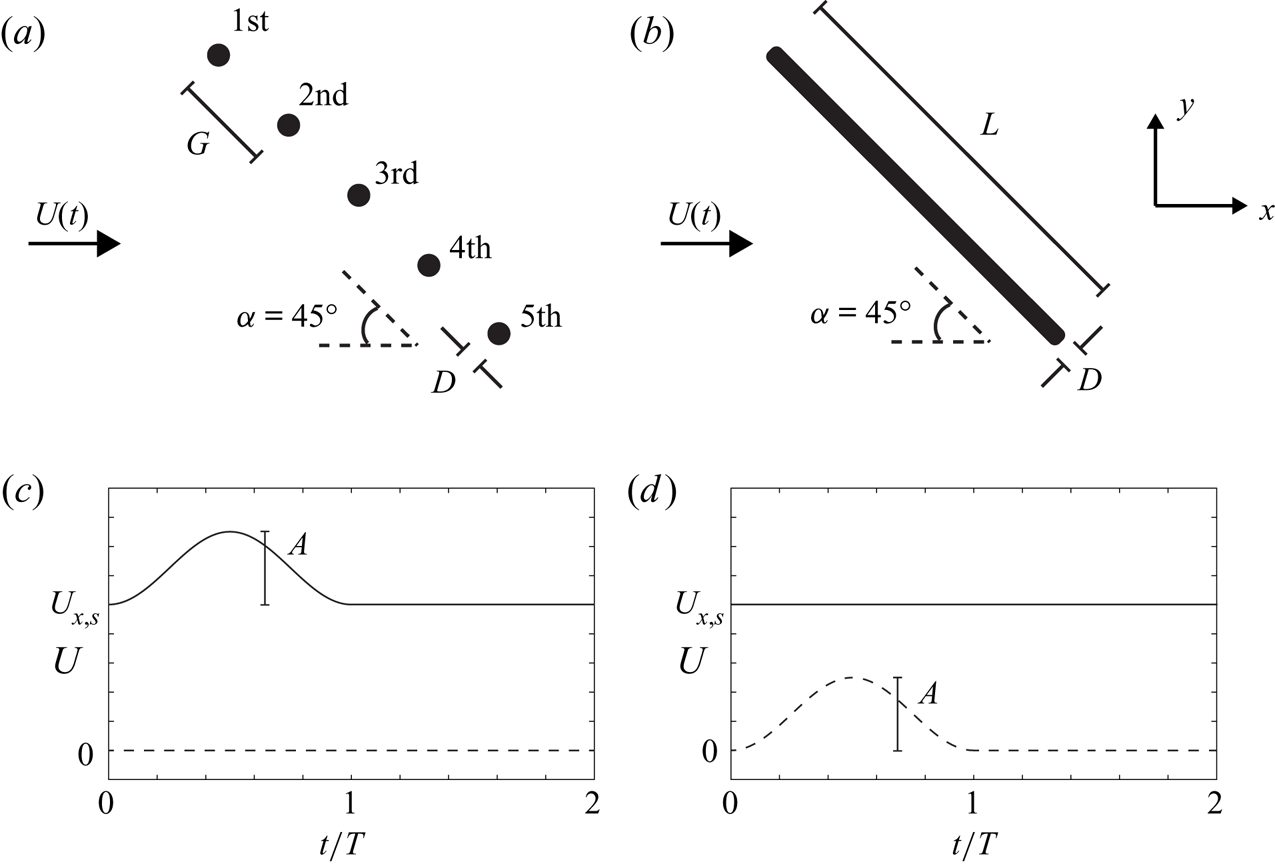
The study of gusty flows is of great importance for insects with bristled wings because, due to their microscopic body size ( ${<}10^{-3}\ \textrm {m}$), their flight stability is more vulnerable to sudden changes in the flow than typical wings of natural flyers. However, as airflow through the bristled wing surface reduces the drag during the fling process (Santhanakrishnan et al. Reference Santhanakrishnan, Robinson, Jones, Lowe, Gadi, Hedrick and Miller2014), airflow through the gaps is expected to alleviate the undesired forces caused by gusts. That is, a bristled wing configuration itself may function as an intrinsic flight stabilizer, requiring no additional aerodynamic control strategies to dampen the fluctuating forces. In this study, the aerodynamic characteristics of a stationary 2-D bristled wing subjected to a single intermittent head-on gust with a sinusoidal velocity profile are numerically investigated for a wide range of parameters, including the gust profile, Reynolds number and wing geometry. First, the temporal variation of aerodynamic loading is compared between a 2-D wing model composed of multiple bristles (circular cylinders) and a corresponding flat wing model (figure 1a,b) under an incoming free stream with sinusoidal velocity. The following sections examine the forces exerted on each bristle and the corresponding flow structures during the gust period and discuss the solidities of the virtual fluid barriers and their effects on aerodynamic performance. Finally, we introduce a dimensionless parameter that combines the gap width, fluid kinematic viscosity and gust duration in order to characterize the forces exerted on the bristled wing by the unsteady free stream.
Schematic diagrams of (a) a simplified 2-D bristled wing and (b) a corresponding flat wing. Free stream velocity profiles  $U(t)$ with (c)
 $x$- and (d)
 $y$-directional gusts. The solid and dashed lines denote
 $x$- and
 $y$-directional velocity components, respectively. In panels (c,d),
 $A = 0.5 U_{x,{s}}$.

2. Problem description
2.1. Model
As a preliminary study on the aerodynamic response of a bristled wing to a gusty flow, we introduce a simplified 2-D bristled wing model that captures the 2-D features of a biological bristled wing; similar models were also used in recent studies on 2-D bristled wings (Jones et al. Reference Jones, Yun, Hedrick, Griffith and Miller2016; Lee et al. Reference Lee, Lahooti and Kim2018, Reference Lee, Lee and Kim2020). The 2-D assumption seems reasonable in that the aspect ratio of each bristle in an actual bristled wing is sufficiently large. Our model consists of five equally spaced cylinders (bristles) of equal diameter  $D$, which are aligned in a straight line (figure 1a), and the wing model is stationary against a free stream. The diameter of each bristle
 $D$ is 1.0 in our computational domain. The gap width
 $G$ is defined as the distance between the centres of adjacent bristles. That is,
 $G = D$ means that the bristles are in contact. To compare the aerodynamic loadings of bristled wings with those of flat wings with no gaps, the flat wing model of total length (chord)
 $L ({=}4G + D)$ is also introduced (figure 1b). The thickness of the flat wing model is
 $D$. The angle of attack
 $\alpha$ is defined as the angle between the
 $x$-axis and the line connecting the centres of the bristles, and
 $\alpha$ is fixed to
 $45^\circ$ for both wing models. That high angle of attack can be considered as a representative angle of attack during the unsteady flight of insects, and many previous studies on bio-inspired aerodynamics have considered the high angle of attack range around
 $45^\circ$ (e.g. Dickinson et al. Reference Dickinson, Lehmann and Sane1999; Birch & Dickinson Reference Birch and Dickinson2003; Santhanakrishnan et al. Reference Santhanakrishnan, Robinson, Jones, Lowe, Gadi, Hedrick and Miller2014).
Initially, a steady-state flow is established around the wing model for a uniform free stream with speed  $U_{x,{s}}$. The basic steady flow speed
 $U_{x,{s}}$ is normalized with respect to a reference speed
 $U_0$:
 $U_0 = 1$ in our numerical set-up. A single intermittent gust with a sinusoidal velocity profile is suddenly introduced to the free stream during the period
 $t = 0$–
 $T$. Because of the small length scale of a biological bristled wing (
 ${<}10^{-3}\ \textrm {m}$), we assume that the gust is spatially uniform in either the
 $x$- or
 $y$-direction. The time-dependent inlet velocity profile of the
 $x$-directional gust is set to be
 \begin{gather} \boldsymbol{U}(t) = \left[U_{x,{s}} + \frac{A}{2} + \frac{A}{2}\sin\left(\frac{2{\rm \pi} t}{T}- \frac{\rm \pi}{2}\right)\right]\boldsymbol{i}, \quad t \in [0,T] \end{gather}
 \begin{gather}\boldsymbol{U}(t) = U_{x,{s}}\boldsymbol{i}, \quad t \in [T,\infty] \end{gather}
where  $A$ and
 $T$ are the maximum velocity amplitude and duration of the gust, respectively (figure 1c). After
 $t = T$, the free stream velocity returns to the constant value
 $U_{x,{s}}$. In a similar manner, a
 $y$-directional gust added to the
 $x$-directional uniform free stream is given as
 \begin{gather} \boldsymbol{U}(t) = U_{x,{s}}\boldsymbol{i} + \left[\frac{A}{2} + \frac{A}{2}\sin \left(\frac{2{\rm \pi} t}{T}-\frac{\rm \pi}{2}\right)\right]\boldsymbol{j}, \quad t \in [0,T] \end{gather}
 \begin{gather}\boldsymbol{U}(t) = U_{x,{s}}\boldsymbol{i}, \quad t \in [T,\infty]. \end{gather}
This study primarily considers the  $x$-directional gust (2.1), and the
 $y$-directional gust (2.2) is used for only a few cases. The
 $y$-directional gust is considered only to demonstrate the linearity of the governing equations for a creeping flow in § 3.4. Note that
 $\alpha$ is still defined as
 $45^\circ$ for the cases with the
 $y$-directional gust although the
 $y$-directional gust changes the effective angle of attack.
For bristled wings in nature, the range of the Reynolds number based on the reference speed  $U_0$,
 $Re = DU_0/\nu$, was estimated to be 0.01–0.1 (Jones et al. Reference Jones, Yun, Hedrick, Griffith and Miller2016). Additionally, the dimensionless gap width
 $G/D$ has been reported to be around 10 (Jones et al. Reference Jones, Yun, Hedrick, Griffith and Miller2016). Unfortunately, regarding the dimensionless gust duration
 $TU_0/D$ and dimensionless maximum velocity amplitude of a gust
 $A/U_0$, there is little information on what kinds of gust microscopic insects with bristled wings are likely to be exposed to in the natural environment; here, the dimensionless gust duration represents the ratio of the gust time scale
 $T$ to the convection time scale
 $D/U_0$. Keeping their feasible flight environments and morphological characteristics in mind to a certain extent, we consider large variations in the orders of the parameters. For the bristled wing models in this study,
 $G/D$,
 $DU_0/\nu$ and
 $TU_0/D$ have large variations in their order of magnitude, with
 $G/D$ ranging from 3–200,
 $DU_0/\nu$ ranging from 0.01–0.1, and
 $TU_0/D$ ranging from 1–100. Although the range of
 $G/D$ has been reported to be around 10 for the insects, the large range of
 $G/D$ in this study is intended to characterize unsteady force fluctuations with an appropriate dimensionless parameter, which will be introduced in § 3.5. In this study,
 $A/U_0$ and
 $U_{x,{s}}/U_0$ are mainly fixed to 0.5 and 1.0, respectively. To check the linearity of the governing equations for a creeping flow, we vary
 $A/U_0$ from 0.1–0.5 and
 $U_{x,{s}}/U_0$ from 0–1.0 for a few cases in § 3.4. The large variations in the orders of these parameters allow us to examine the transition in the solidity of the virtual fluid barriers during the gust period.
2.2. Numerical method
The governing equations for a 2-D incompressible laminar flow were solved numerically using OpenFOAM. To ensure an initial steady-state solution at  $t = 0$, the simpleFoam solver and the second-order (Gauss linear) scheme for spatial discretization were used, and the time derivative was set to be zero for the steady-state solution. Thereafter, for a transient solution (
 $t > 0$), the pisoFoam solver was adopted with the second-order (Gauss linear) spatial and first-order (Euler) temporal discretization schemes implemented.
The entire computational domain is rectangular with  $[-2.5\times 10^5D, 2.5\times 10^5D] \times [-2.5\times 10^5D, 2.5\times 10^5D]$. Near each bristle surface 10 layers of structured grids were constructed, and the size of the grids adjacent to the bristle surface was fixed to
 $0.01D$. Outside the structured grids, we constructed unstructured triangular grids with exponentially increasing sizes from the structured layers. The growth ratio of the grid size was 1.05 for the rectangular region encompassing the bristles, and the maximum grid size within this region is limited to
 $5D$. The size of this rectangular region depends on the gap width
 $G$. For the rest of the computational domain, structured rectangular grids were constructed with exponentially increasing sizes of the growth rate 1.05. The total number of grids ranged from
 $1.0\times 10^5$ to
 $2.0\times 10^5$, depending on
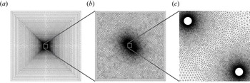
 $G$. Figure 2 illustrates the computational grids for a bristled wing with
 $G/D = 9$ as an example. The large domain size was intended to minimize any error caused by artificial boundary conditions (Lange, Durst & Breuer Reference Lange, Durst and Breuer1998). A no-slip condition is applied on the bristle surfaces. For the cases with the
 $x$-directional gust, the time-dependent velocity (2.1) and the pressure gradient of
 $\partial p/\partial n = -\textrm {d}U_n(t)/\textrm {d}n$ are imposed at the inlet, where
 $n$ is the direction normal to the boundary. The zero normal gradients of velocity and zero pressure are imposed at the outlet. The zero normal velocity and zero normal gradients of all variables are imposed at the top and bottom boundaries. For the case with the
 $y$-directional gust, the time-dependent velocity (2.2) and the pressure gradient of
 $\partial p/\partial n = -\textrm {d}U_n(t)/\textrm {d}n$ are imposed for the four outer boundaries of the domain.
Computational grids for a bristled wing with  $G/D=9$.

To determine the grid size and the computational time step, a simple convergence test was conducted for a single isolated circular cylinder under a purely gusty flow without a constant free stream component in (2.1):  $U_{x,{s}} = 0$. We varied the minimum grid size from
 $0.01D$ to
 $0.02D$ and the time step from
 $0.002T$ to
 $0.004T$, while keeping all other conditions unchanged. For
 $DU_0/\nu = 1$,
 $TU_0/D = 1$ and
 $A/U_0 = 0.5$, the difference in the maximum
 $x$-directional forces on the single isolated cylinder due to the gusty flow was less than 0.2
 $\%$ between the two cases. This convergence test justifies our decision to set the minimum grid size and the time step to
 $0.01D$ and
 $0.002T$, respectively. For the flat wing model, the minimum size of the grid near the wing surface was fixed to
 $0.1D$. For the case of a large
 $T$, the time step was restricted to ensure that the Courant number did not exceed 0.5.
To validate our numerical method, we simulated a planar harmonic oscillatory flow around a fixed circular cylinder. In this validation test, some parameters differed from those defined in § 2.1. A stationary cylinder was subjected to a periodic flow  $\boldsymbol {U}(t) = A \sin (2{\rm \pi} t/T)\boldsymbol {i}$, where
 $A$ and
 $T$ are the velocity amplitude and period of the oscillatory flow. The Keulegan–Carpenter number
 $KC = AT/D$ and the viscous scale parameter
 $\beta = D^2/\nu T$ were 1 and 76, respectively;
 $\nu$ is the fluid kinematic viscosity and
 $D$ is the cylinder diameter. The same numerical set-ups and grid configurations as described above were employed, and 5000 time steps were assigned for each cycle. The time history of the in-line force (drag) coefficient
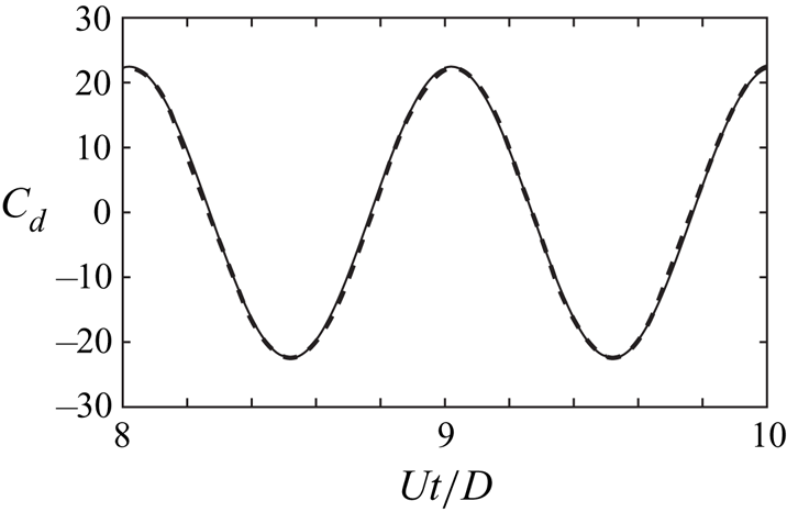
 $C_d(t) = 2 F_x(t)/\rho A^2D$ is compared with that of Lin et al. (Reference Lin, Bearman and Graham1996) in figure 3, and they are in excellent agreement. For example, the maximum values of
 $C_d(t)$ during each cycle are 22.3 and 22.5 in Lin et al. (Reference Lin, Bearman and Graham1996) and this study, respectively.
Time history of in-line force coefficient  $C_d$ for a fixed cylinder in oscillatory flow (
 $KC = 1$ and
 $\beta = 76$): solid line (present study) and dashed line (Lin, Bearman & Graham Reference Lin, Bearman and Graham1996).

3. Results and discussion
3.1. Comparison between flat and bristled wings
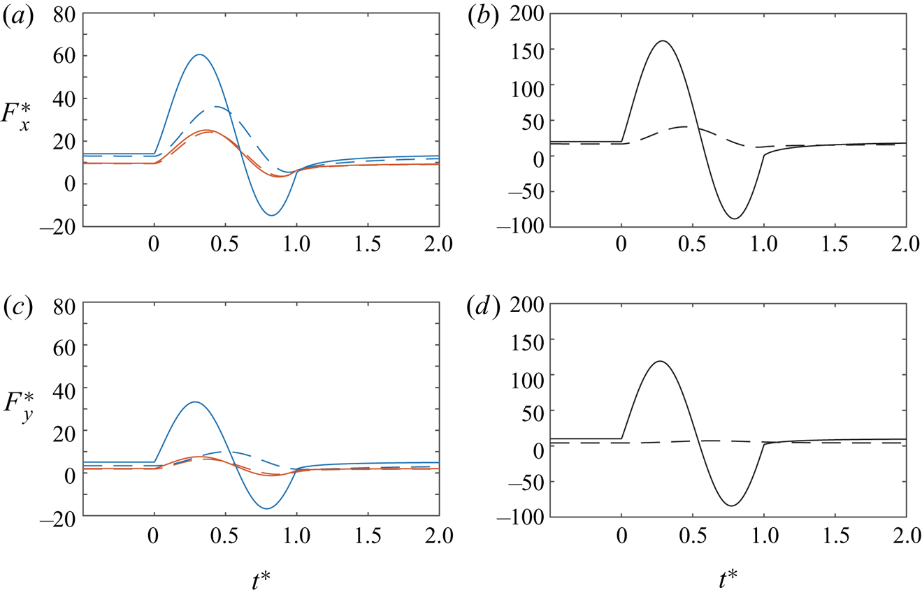
In this section, we report the different aerodynamic responses of the two distinct types of wings under gusty flows. We first begin by comparing the force exerted on the bristled and flat wings with the time-dependent inlet velocity profile of (2.1) and a representative combination of the parameters,  $DU_0/\nu = 0.1$,
 $TU_0/D = 10$,
 $U_{x,{s}}/U_0 = 1$ and
 $A/U_0 = 0.5$ (figure 4). The aerodynamic performance of a bristled wing in a gusty flow will be discussed for a wide range of parameters in the following sections. The
 $x$-directional (
 $F_x$, drag) and
 $y$-directional (
 $F_y$, lift) forces on the flat and bristled wings are made dimensionless using
 $\mu$,
 $A$, and
 $D$:
 $F^*_x = F_x /\mu AD$ and
 $F^*_y = F_y /\mu AD$. Note that the velocity amplitude
 $A$ of the gust is considered when defining the dimensionless forces because our primary interests are the forces generated by a gust; § 3.4 describes why the unsteady force fluctuations produced by the gust are better characterized by
 $A$ rather than
 $U_{x,{s}}$. In addition, the dimensionless time is defined as
 $t^* = t/T$. For a small gap width, the aerodynamic forces of the bristled wing are comparable to those of the flat wing in the steady state before the streamwise gust is imposed (
 $t^* \leqslant 0$) (Sunada et al. Reference Sunada, Takashima, Hattori, Yasuda and Kawachi2002; Lee & Kim Reference Lee and Kim2017; Lee et al. Reference Lee, Lee and Kim2020). For example, the
 $F^*_x$ values of the bristled and flat wings are 9.48 and 9.65 for
 $G/D = 3$, 13.0 and 14.1 for
 $G/D = 9$, 16.8 and 20.1 for
 $G/D = 20$, respectively (figure 4a,b); the drag force ratios of the bristled wing over the flat wing are 0.98, 0.92 and 0.84 for
 $G/D = 3$,
 $9$ and
 $20$, respectively. Similarly, the
 $F^*_y$ values of the bristled and flat wings are 1.90 and 2.07 for
 $G/D = 3$, 3.41 and 5.51 for
 $G/D = 9$, 4.18 and 10.14 for
 $G/D = 20$, respectively (figure 4c,d); the corresponding lift force ratios between the two models are 0.91, 0.67 and 0.42, respectively.
(a,b) Dimensionless drag  $F^*_x = F_x/\mu A D$ and (c,d) dimensionless lift
 $F^*_y = F_y/\mu A D$ of the bristled and flat wing models with the time-dependent inlet velocity profile of
 $U(t)$ (2.1):
 $DU_0/\nu = 0.1$,
 $TU_0/D = 10$,
 $U_{x,{s}}/U_0 = 1$ and
 $A/U_0 = 0.5$. The dashed and solid lines denote the bristled wing and the flat wing, respectively. Panels (a,c) show the cases when
 $G/D = 3$ (red) and 9 (blue), whereas panels (b,d) show the case when
 $G/D = 20$ (black). Note that the ranges of the
 $y$-axis differ between panels (a,c) and panels (b,d).

The forces on both types of wing fluctuate as they encounter the streamwise gust ( $t^* \geqslant 0$) and eventually recover their steady-state values after the gust recedes. Notably, the force fluctuations of the bristled wing are smaller than those of the flat wing (figure 4). Although the streamwise velocity component does not become negative, negative drag and lift forces can occur for some flat wing models; this does not occur for the bristled wing. The difference in
 $F^*_x$ (and
 $F^*_y$) between the two types of wing becomes greater with the gap width. To quantify the variation in the forces under the gusty flow and under the steady state, we define the deviation in
 $F^*_x$ (and
 $F^*_y$) as
 $\Delta F^*_x$ (and
 $\Delta F^*_y$) as follows:
 \begin{equation} \Delta F^*_x = \frac{(F_x - F_{x,{s}})}{\mu AD} \quad \textrm{and} \quad \Delta F^*_y = \frac{(F_y - F_{y,{s}})}{\mu AD}, \end{equation}
where  $F_{x,{s}}$ and
 $F_{y,{s}}$ are the
 $x$- and
 $y$-directional steady-state forces obtained at
 $t^* = 0$. For the flat wings, the maximum
 $\Delta F^*_x$ values at
 $t^* > 0$ are 15.5, 46.4 and 141.6 for
 $G/D = 3$,
 $9$ and
 $20$, respectively. For the bristled wings, they are 14.7, 23.2 and 24.0 for
 $G/D = 3$,
 $9$ and
 $20$, respectively. Therefore, the ratios of maximum
 $\Delta F^*_x$ for the bristled wing over that for the flat wing are 0.95 for
 $G/D = 3$ and 0.17 for
 $G/D = 20$. At
 $G/D = 20$, the maximum
 $\Delta F^*_x$ value of the bristled wing is less than one-fifth of that of the flat wing. This ratio is much smaller than the value of 0.84 at the steady state (
 $t^* = 0$). Similarly, the minimum
 $\Delta F^*_x$ also exhibits a greater difference at larger gap widths. For example, at
 $G/D = 20$, the minimum
 $\Delta F^*_x$ value of the flat wing is
 $-108.6$, whereas that of the bristled wing is
 $-4.7$.
For the bristled wing, the attenuation in the fluctuating force caused by the gust is more pronounced in the lift force  $F_y$ perpendicular to the direction of the gust (figure 4c,d). For example, the maximum
 $\Delta F^*_y$ values of the bristled and flat wings are 4.55 and 5.56 for
 $G/D = 3$, 6.52 and 28.2 for
 $G/D = 9$, 2.97 and 109.0 for
 $G/D = 20$, respectively. Interestingly, the ratio of the two values for
 $G/D = 20$ is only 0.027; note that the ratio is reported to be 0.17 for the drag force
 $\Delta F^*_x$. Similarly, the minimum lift forces of the bristled wing show significantly attenuated values compared with those of the flat wing. The minimum
 $\Delta F^*_y$ values of the bristled and flat wings are
 $-1.7$ and
 $-21.9$ for
 $G/D = 9$. In addition, when
 $G/D = 20$, no minimum peak value in
 $\Delta F^*_y$ even appears for the bristled wing. Instead, it slightly increases and then asymptotically converges back to the steady-state value. In this case, the bristled wing barely notices the gust in terms of lift fluctuations.
The discontinuities in the slope of the force curves are observed at  $t^* = 0$ and
 $1$ for the flat wing model (figure 4). This is primarily because the acceleration of the free stream,
 $\textrm {d}U_x(t)/\textrm {d}t$, and the resultant added-mass force has the discontinuities in their slopes at
 $t^* = 0$ and
 $1$. Such sudden changes in the forces at
 $t^* = 0$ and
 $1$ are annihilated for the bristled wing models. The results presented in figure 4 suggest that, in gusty environments, insects with bristled wings experience smaller fluctuations in forces than insects with flat continuous wings, enabling more stable flight.
The time-dependent flow structures around the bristled and flat wings at several time instants illustrate the aforementioned differences in the force responses between the two types of wing (figure 5). In figure 5, the gust profile is given as (2.1) with  $DU_0/\nu = 0.1$,
 $TU_0/D = 10$,
 $U_{x,{s}}/U_0 = 1$ and
 $A/U_0 = 0.5$, which are the same parameters as in figure 4. The flow structures between the two types of wing are compared for
 $G/D = 9$ as a representative case. To quantify how much fluid leaks through the gaps, we define the flow rate
 $Q$ at each gap as
 \begin{equation} Q=\int_l \boldsymbol{n} \boldsymbol{\cdot} \boldsymbol{u}\,\textrm{d}l, \end{equation}
where  $\boldsymbol {u}$ is the velocity vector in the fluid domain,
 $l$ is the line connecting the centres of neighbouring bristles and
 $\boldsymbol {n}$ is the unit vector perpendicular to the line
 $l$. The flow rate
 $Q$ through a single gap is made dimensionless with respect to
 $G$ and
 $U_0$:
 $Q/GU_0$.
Vorticity contours of (a) the bristled wing ( $G/D = 9$) and (b) the flat wing with the time-dependent inlet velocity profile of (2.1):
 $DU_0/\nu = 0.1$,
 $TU_0/D = 10$,
 $U_{x,{s}}/U_0 = 1$ and
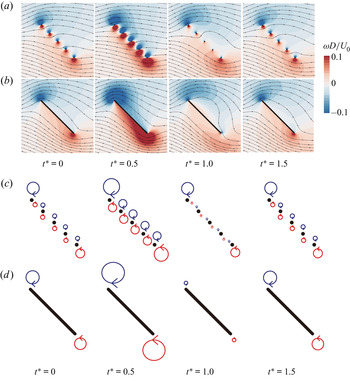
 $A/U_0 = 0.5$. In panels (a,b), streamlines are depicted on vorticity contours. (c,d) Schematic diagrams for the evolution of the vortical structures corresponding to panels (a,b), respectively. The arrows indicate the rotating direction of the vortex. For panels (a,b), see supplementary movie 1 available at https://doi.org/10.1017/jfm.2020.1155.

At  $t^* = 0$, because of strong viscous diffusion, the vorticity in a certain gap is annihilated by the vorticity with the opposite sign that is formed by the adjacent bristle. Thus, the vorticity between the gaps is weaker than the vorticity at the outer edges of the wing (figure 5a,b). The size and magnitude of the outer-edge vortices of the bristled wing for
 $G/D = 9$ are comparable to those of the flat wing depicted in figure 5(b). Additionally, for
 $G/D = 9$, the
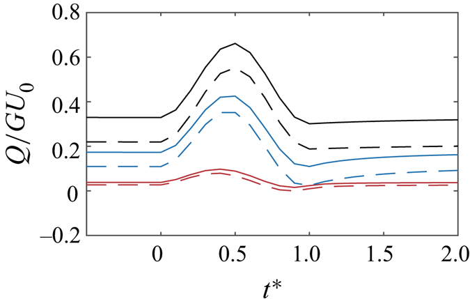
 $Q/GU_0$ values of the first and fourth gaps are 0.17 and 0.11 at
 $t^* = 0$, respectively (figure 6); here, the first and fourth gaps indicate the gap between the first and second bristles and the gap between the fourth and fifth bristles, respectively (figure 1). Such small values of
 $Q/GU_0$ indicate that strong flow blockage occurs within the gaps of the bristled wing. These results reflect the well known features of a bristled wing subjected to a steady low-Reynolds-number flow (Sunada et al. Reference Sunada, Takashima, Hattori, Yasuda and Kawachi2002; Lee & Kim Reference Lee and Kim2017; Lee et al. Reference Lee, Lee and Kim2020).
Time history of dimensionless flow rate  $Q/GU_0$ through the gaps of the bristled wing:
 $DU_0/\nu =0.1$,
 $TU_0/D = 10$,
 $U_{x,{s}}/U_0 = 1$ and
 $A/U_0 = 0.5$. The solid and dashed lines represent the flow rates obtained at the first and fourth gaps, respectively:
 $G/D = 3$ (red);
 $9$ (blue);
 $20$ (black).

However, as the wings encounter gusts, the flow structures of both wing models become distinctive, which underlies the attenuated forces of the bristled wing during the gust period ( $0 \leqslant t^* \leqslant 1.0$). At
 $t^* = 0.5$, when the free stream speed reaches its peak (figure 1c), the vortices in the gaps of the bristles and the outer-edge vortices are strongly developed (figure 5a,c). The
 $Q/GU_0$ values of the first and fourth gaps are 0.42 and 0.35 at
 $t^* = 0.5$, respectively, which are more than twice the magnitudes in the steady state at
 $t^* = 0$ (figure 6). The increments in
 $Q/GU_0$ from
 $t^* = 0$ to
 $0.5$ are 0.25 and 0.24 for the first and fourth gaps, respectively. That is, almost half of the gusty flow with velocity amplitude
 $A$ can leak through the gaps additionally; the velocity amplitude
 $A/U_0$ of the gust is 0.5. On the other hand, in the case of the flat wing, all the fluid must flow around the outermost edges of the wing, because the fluid cannot penetrate the wing surface. Therefore, during the gust period, the leading- and trailing-edge vortices of the flat wing are more strongly developed than those of the bristled wing (figure 5b,d). The impingement of the incoming fluid on the flat wing, which should eventually detour the wing, produces an augmented aerodynamic loading compared with the bristled wing.
When the incident flow decelerates after the peak in the free stream speed ( $t^* \geqslant 0.5$), the vortical structures that have strongly developed in the accelerating phase are mitigated (figure 5a,c). The mechanism here is quite analogous to the process of stopping-vortex formation reported by Kim & Gharib (Reference Kim and Gharib2011) and Lee et al. (Reference Lee, Lahooti and Kim2018). For the bristled wing, the leading- and trailing-edge vortices and the vortices in the gaps become less severe and weaker than those in the steady state (
 $t^* = 0$). Similarly, the strengths of the leading- and trailing-edge vortices of the flat wing decrease as well (figure 5b,d). The changes in strength of both vortices over time are much greater in the flat wing than in the bristled wing that allows fluid leakage through the gaps. The outer-edge vortices of the flat wing, which were stronger than those of the bristled wing at
 $t^* = 0.5$, become weaker than in the bristled wing at
 $t^* = 1.0$. For the flat wing, a significant variation in the vortical structure over the gust period (
 $0 \leqslant t^* \leqslant 1.0$) results in notable variations in the forces acting on the wing (figure 4). The effects of the gust almost disappear at
 $t^* = 1.5$, and both the flow structure and the aerodynamic forces almost recover to their steady-state values.
Regarding the flow rate through the gaps for gap widths other than  $G/D = 9$, the increments in
 $Q/GU_0$ from
 $t^* = 0$ to
 $0.5$ are 0.051 and 0.041 for the first and fourth gaps of the
 $G/D = 3$ case, respectively. The corresponding increments in
 $Q/GU_0$ are 0.33 for both the first and fourth gaps of the
 $G/D = 20$ case (figure 6). Although the flow fields for the bristled wings with
 $G/D = 3$ and
 $20$ are not presented in figure 5, the bristled wing with
 $G/D = 3$ exhibits the strong effect of the virtual fluid barrier during the gust period, yielding negligible increments in
 $Q/GU_0$. In contrast, the formation of the virtual fluid barrier is relatively weak for the bristled wing with
 $G/D = 20$, and the leakage through the gaps is more prominent than with
 $G/D = 9$, followed by a significant increment in
 $Q/GU_0$.
In steady low-Reynolds-number flow, bristled wings form a fully developed virtual fluid barrier in the gaps and thereby allow only a small volume of fluid through the gaps, resulting in aerodynamic forces comparable to those of flat wings (Sunada et al. Reference Sunada, Takashima, Hattori, Yasuda and Kawachi2002; Lee & Kim Reference Lee and Kim2017; Lee et al. Reference Lee, Lee and Kim2020). When the gust blows for a short duration, the fluid barrier does not become fully developed in response to the gust; some time is required for the development of the fluid barrier. Thus, during the gust, the fluid flow can penetrate the gaps more easily, which alleviates the undesirable aerodynamic forces generated by the gust. The preliminary examination reported in this section shows that a reduction in aerodynamic force fluctuation is more significant for the bristled wing, and that the reduction depends on the gap width. The combined effects of the gap width, fluid kinematic viscosity and gust duration on the force fluctuation will be discussed in more detail in § 3.5.
3.2. Aerodynamics of individual bristles
In § 3.1, we reported that the bristled wing had an advantage over the flat wing in that it could alleviate the unsteady aerodynamic loading caused by abrupt changes in the free stream velocity. As a next step, the aerodynamics of individual bristles with various gap widths should be examined to elucidate the force-damping mechanisms of the bristled wing, which are correlated with the effectiveness of the virtual fluid barriers.
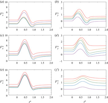
The deviation in force from the steady-state value, (3.1a,b), is again used to characterize the force fluctuation of each bristle. For each bristle, the maximum  $\Delta F^*_x$ value gradually converges to a certain value as
 $G/D$ increases (figure 7a,c,e). For example, when the gap width
 $G/D$ increases from 3 to 9, the maximum
 $\Delta F^*_x$ value of the first bristle increases from 3.76 to 4.75. Moreover, when
 $G/D$ changes from 9 to 20, the increment in the maximum
 $\Delta F^*_x$ value is only approximately 0.03, from 4.75 to 4.78. For
 $G/D = 20$, the maximum
 $\Delta F^*_x$ values of all the bristles reside in a narrow range of 4.78–4.81. Before converging to the same value as for the single isolated bristle with increasing gap width, the maximum
 $\Delta F^*_x$ values for the two outermost bristles are greater than those of the inner bristles; see the cases of
 $G/D = 3$ and
 $9$ (figure 7a,c).
Dimensionless drag  $F^*_x$ and lift
 $F^*_y$ of individual bristles with the time-dependent inlet velocity profile of
 $U(t)$ (2.1):
 $DU_0/\nu = 0.1$,
 $TU_0/D = 10$,
 $U_{x,{s}}/U_0 = 1$ and
 $A/U_0 = 0.5$. Panels (a,b), (c,d) and (e,f) show the cases of
 $G/D = 3$,
 $9$ and
 $20$, respectively. Colour coding is as follows: first bristle (red); second bristle (orange); third bristle (green); fourth bristle (blue); fifth bristle (purple). The ranges of the
 $y$-axis differ between panels (a,c,e) and panels (b,d,f).

On the other hand, for each bristle, the maximum  $\Delta F^*_y$ values tend to increase and then decrease with
 $G/D$, exhibiting a peak when
 $G/D$ is between 3 and 20 (figure 7b,d,f). After the peak,
 $\Delta F^*_y$ asymptotically tends to zero as
 $G/D$ goes to infinity. Here, we identify two unique features of the forces that do not appear when the bristled wing is subjected to a steady incoming flow. First, the orders of the
 $F^*_y$ values at the steady state (
 $t^* = 0$) and the
 $\Delta F^*_y$ values during the gust period are clearly different. The
 $F^*_y$ value of each bristle at the steady state decreases sequentially from the first to fifth bristle for
 $G/D = 3$,
 $9$ and
 $20$. For the steady incoming flow, this trend is observed regardless of the gap width (Lee et al. Reference Lee, Lee and Kim2020). In contrast, while the maximum
 $\Delta F^*_y$ values decrease sequentially from the first to fifth bristle for
 $G/D = 3$, the inner bristles experience greater maximum
 $\Delta F^*_y$ values than the outermost bristles for
 $G/D = 9$ and
 $20$; note that, as mentioned in the previous paragraph, the orders of
 $\Delta F^*_x$ do not change with increasing gap width. A second feature is that all the bristles produce large values of maximum
 $\Delta F^*_y$ during the gust period. For example, the maximum
 $\Delta F^*_y$ value of the fifth bristle is
 $56\,\%$ of the first bristle for
 $G/D = 3$ and
 $69\,\%$ for
 $G/D = 20$. Meanwhile, the fifth bristle in the steady incoming flow (
 $t^* = 0$) produces nearly zero or negative lift (figure 7b,d,f).
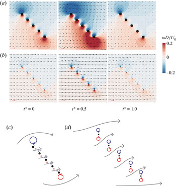
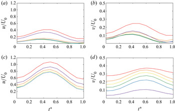
The aforementioned unique features of the forces on individual bristles are correlated with flow velocities near the bristles because they directly reflect the formation of virtual fluid barriers. For the bristled wing with  $G/D = 3$, virtual fluid barriers are strongly formed during the gust period. At
 $t^* = 0.5$, therefore, most of the incoming flow passes around the outermost edges (leading edge and trailing edge) of the wing, rather than through the gaps (figure 8a,c); in this study, the leading and trailing edges indicate the first and fifth bristles, respectively. The time histories of
 $u/U_0$ and
 $v/U_0$ are also presented at specific points for the leading and trailing edges as well as for the centres of the four gaps (figure 9). The specific points for the leading and trailing edges are positioned above the first bristle and below the fifth bristle, respectively, at a distance of
 $0.5G$ along the straight line connecting the centres of the five bristles. The increments in
 $u/U_0$ and
 $v/U_0$ at the leading and trailing edges from
 $t^* = 0$ to
 $0.5$ are greater than those inside the gaps (figure 9a,b). For example, the increment in
 $u/U_0$ from
 $t^* = 0$ to
 $0.5$ is 0.22 for the leading edge, but just 0.08 for the first gap (figure 9a). Because of the strong formation of virtual fluid barriers during the gust period, the bristled wing with
 $G/D = 3$ presents similar force generation behaviour in the middle of the gust period (
 $t^* = 0.5$) to that observed in the steady state (
 $t^* = 0$); the drag forces
 $\Delta F^*_x$ of the inner bristles are smaller than those of the outermost bristles, and the lift forces
 $\Delta F^*_y$ decrease sequentially from the first to the fifth bristle.
Velocity magnitude contours of the bristled wing for (a)  $G/D = 3$ and (b)
 $G/D = 20$:
 $DU_0/\nu =0.1$,
 $TU_0/D = 10$,
 $U_{x,{s}}/U_0 = 1$ and
 $A/U_0 = 0.5$. The contours are superimposed with velocity vectors. The red arrow in the lower left-hand corner of each contour is a unit vector of magnitude
 $U_0$. Note that the size of the bristle is actually the same between panels (a,b) and the fluid domain in panel (b) is much greater than the fluid domain in panel (a). (c,d) Schematic diagrams for the vortical structures corresponding to panels (a,b) at
 $t^* = 0.5$, respectively. The blue and red arrows indicate the rotating direction of the vortex. The grey arrows indicate the instantaneous fluid motions. For panels (a,b), see supplementary movie 2.

Time histories of  $x$- and
 $y$-directional velocity components,
 $u/U_0$ and
 $v/U_0$, for (a,b)
 $G/D = 3$ and (c,d)
 $G/D = 20$ at the points for the leading and trailing edges as well as the centres of the gaps:
 $DU_0/\nu =0.1$,
 $TU_0/D = 10$,
 $U_{x,{s}}/U_0 = 1$ and
 $A/U_0 = 0.5$. Panels (a,c) show
 $u/U_0$ while panels (b,d) show
 $v/U_0$. The colour coding is as follows: leading edge (red); first gap (orange); second gap (yellow); third gap (green); fourth gap (blue); trailing edge (purple). The ranges of the
 $y$-axis differ between panels (a,c) and panels (b,d).

The virtual fluid barrier is not immediately fully formed in accordance with the increase in the free stream velocity from  $1.0U_0$ to
 $1.5U_0$. Thus, the local flow velocities around the wing at
 $t^* = 0.5$ with the instantaneous free stream velocity
 $1.5U_0$ are greater than those obtained with the uniform steady free stream with the same inlet velocity of
 $1.5U_0$. At
 $t^* = 0.5$, the
 $u/U_0$ and
 $v/U_0$ values in the gap, as well as at the leading and trailing edges, are approximately double (or more) those at
 $t^* = 0$ (figure 9a,b). These increments are significant, considering that the free stream velocity changes from
 $U_0$ at
 $t^* = 0$ to
 $1.5U_0$ at
 $t^* = 0.5$. In the same manner, the forces on the bristles are augmented by the increase in the local flow velocities near the bristles. This is why even the fifth bristle is subjected to large positive lift fluctuations
 $\Delta F^*_y$.
As the effects of the virtual fluid barriers are weakened by enlarging the gap width, the incoming flow does not pass over the outermost edges of the wing, but rather passes through the gaps. Inside the gaps in the  $G/D = 20$ case, the increments in
 $u/U_0$ from
 $t^* = 0$ to
 $0.5$ are close to 0.5, which is comparable to the gust velocity amplitude
 $A/U_0 = 0.5$ (figure 9c). The increments in
 $u/U_0$ at the leading and trailing edges during the corresponding period are also around 0.5. Unlike the
 $G/D = 3$ case, vortices with opposite signs that develop at each gap do not cancel each other out (figure 8b,d). Instead, symmetrical vortical structures develop independently between the upper and lower surfaces of each bristle, and the magnitudes are similar to those generated at the leading and trailing edges. Because the vortices of each bristle develop almost independently, the drag force fluctuation
 $\Delta F^*_x$ of each bristle converges to that of a single isolated bristle (figure 7e). However, with the vortical configuration at
 $t^* = 0.5$, the
 $y$-directional fluid motions induced at the gaps are more significant than those induced at the leading and trailing edges as depicted in figure 8(d). The increments in the
 $v/U_0$ values at the gaps from
 $t^* = 0$ to
 $0.5$ are approximately twice the size of those at the leading and trailing edges (figure 9d). For this reason, the inner bristles experience greater lift fluctuations
 $\Delta F^*_y$ than the outermost bristles (figure 7f).
3.3. 25-bristle model
The findings that we reported with the five-bristle model in the previous sections can be extended to the model composed of a larger number of bristles. To demonstrate their generality, a 25-bristle model is considered as a representative case only in this section. Similar to the five-bristle model, the 25-bristle model consists of 25 equally spaced bristles (figure 10a). For this model, we use the time-dependent inlet velocity profile of (2.1) and a representative combination of the parameters,  $DU_0/\nu = 0.1$,
 $TU_0/D = 10$,
 $U_{x,{s}}/U_0 = 1$ and
 $A/U_0 = 0.5$, and the gap width
 $G/D$ is fixed to be 9.
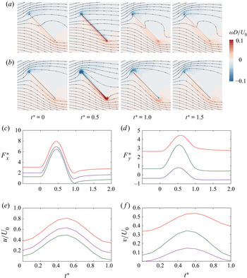
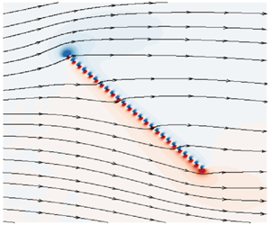
Vorticity contours of (a) the 25-bristle model ( $G/D = 9$) and (b) the corresponding flat wing with the time-dependent inlet velocity profile of (2.1):
 $DU_0/\nu = 0.1$,
 $TU_0/D = 10$,
 $U_{x,{s}}/U_0 = 1$ and
 $A/U_0 = 0.5$. In panels (a,b), streamlines are depicted on the vorticity contours. (c,d) Dimensionless drag
 $F^*_x$ and lift
 $F^*_y$ of individual bristles in the 25-bristle model. The colour coding is as follows: first bristle (red); 13th bristle (green); 25th bristle (purple). (e,f) Time histories of
 $x$- and
 $y$-directional velocity components,
 $u/U_0$ and
 $v/U_0$, for the 25-bristle model. The colour coding is as follows: leading edge (red); 13th gap (green); trailing edge (purple). The ranges of the
 $y$-axis differ between panels (c,d) and panels (e,f).

In common with the five-bristle model, the force fluctuations of the 25-bristle model are smaller than those of the flat wing. The ratios of maximum  $\Delta F^*_x$ and
 $\Delta F^*_y$ for the bristled wing over those for the flat wing are 0.17 and 0.09, respectively. These ratios are much smaller than the values of 0.97 and 0.70, respectively, at the steady state (
 $t^* = 0$). The time-dependent flow structures around the bristled and flat wings are presented at several time instants (figure 10a,b). The overall trends of the 25-bristle model are analogous to those of the five-bristle model. For the bristled wing at
 $t^* = 0.5$, the vortices in the gaps of bristles, as well as the outer-edge vortices, are strongly developed in response to the gust, and they become annihilated after
 $t^* = 0.5$ (figure 10a). Compared with
 $t^* = 0$ and 1.0, a greater number of streamlines penetrate the gaps of bristles at
 $t^* = 0.5$, indicating that more fluid can leak through the gaps. At the same moment, the outer-edge vortices of the flat wing are more strongly developed than those of the bristled wing because fluids cannot penetrate the wing surface (figure 10b). As we concluded in § 3.1, such significant variations in the vortical structure over the gust period (
 $0 \leqslant t^* \leqslant 1.0$) lead to remarkable variations in the forces acting on the flat and bristled wings.
In addition to the comparison of collective aerodynamic performance between the flat and bristled wings, the aerodynamic behaviours of individual bristles in the 25-bristle model are examined. In figure 7(c), we showed that the maximum  $\Delta F^*_x$ value of each bristle in the five-bristle model with
 $G/D = 9$ was almost the same as that of the single isolated bristle, 4.88. Interestingly, the maximum
 $\Delta F^*_x$ value of each bristle in the 25-bristle model also presents a similar value. For example, the maximum
 $\Delta F^*_x$ values of the first bristle (i.e. the uppermost bristle) in the five- and 25-bristle model are 4.75 and 4.83, respectively, (figures 7c and 10c). Similarly, the
 $\varDelta F^*_x$ values of the bristle at the centre (i.e. the 13th bristle) and the lowermost bristle (i.e. the 25th bristle) in the 25-bristle model are 5.13 and 4.89, respectively (figure 10c). Furthermore, the inner bristle in the 25-bristle model experiences a greater maximum
 $\Delta F^*_y$ value than the outermost bristles (figure 10d), which was also reported for the five-bristle model.
For the five-bristle model, the virtual fluid barriers are not immediately fully formed in accordance with the increase in the free stream velocity by the gust. When the gap width  $G/D$ is large (e.g.
 $G/D = 9$), a significant portion of the incoming flow does not detour around the outermost edges of the five-bristle model, but passes through the gaps during the gust period. Likewise, for the 25-bristle model with
 $G/D = 9$, the increment in
 $u/U_0$ at the 13th gap from
 $t^* = 0$ to 0.5 is 0.39, which is comparable to the gust velocity amplitude
 $A/U_0 = 0.5$ (figure 10e). The increments in
 $u/U_0$ during the corresponding period are also around 0.43 for the leading and trailing edges. The similar increments in
 $u/U_0$ at both the outermost edges and the 13th gap are the consequences of the symmetrical vortical structures developed almost independently in each bristle surface. As we described previously for the five-bristle model, the development of the vortical structures in each gap for
 $t^* = 0\text {--}0.5$ causes more significant
 $y$-directional fluid motions in the gaps than at the leading and trailing edges. The increment in
 $v/U_0$ at the 13th gap from
 $t^* = 0$ to 0.5 is approximately twice those of the leading and trailing edges (figure 10f), and consequently the inner bristle experiences a greater lift fluctuation
 $\Delta F^*_y$ than the outermost bristles (figure 10d).
Regarding the force fluctuations  $\Delta F^*_x$ and
 $\Delta F^*_y$ by the gust and the transient development of gap flows, we found that the five- and 25-bristle models exhibited similar trends and the same aerodynamic principles discussed for the five-bristle model in § 3.2 could be applied to the 25-bristle model. For this reason, the following sections will examine the five-bristle model only because of its simpler configuration.
3.4. Linear property of aerodynamic forces
In the previous sections, the speed of the basic steady flow and the maximum velocity amplitude of the gust have been fixed to  $U_{x,{s}} = 1$ and
 $A = 0.5$, respectively. Because the governing equation for the flow around the bristled wing can be linearized by virtue of the very low-Reynolds-number, our results in the previous sections can be generalized by using this linear property. For the unsteady creeping flow, the convective term in the governing momentum equation can be neglected, provided that
 $DU/\nu < 1$ and
 $D^2/\nu T < 1$ (Maxey & Riley Reference Maxey and Riley1983), where
 $U$ is the free stream speed. In nature, the Reynolds number
 $DU/\nu$ of the smallest insects with bristled wings has been estimated to be around 0.01–0.1 (Jones et al. Reference Jones, Yun, Hedrick, Griffith and Miller2016). Although a reliable range of
 $D^2/\nu T$ for these insects’ habitats is not available,
 $D^2/\nu T <1$ is readily satisfied if
 $T > 10^{-7}\ \textrm {s}$ when we consider the kinematic viscosity
 $\nu$ of air at room temperature and typical bristle diameters of
 $0.5\text {--}2 \times 10^{-6}\ \textrm {m}$ (Jones et al. Reference Jones, Yun, Hedrick, Griffith and Miller2016). Of course, the parameter ranges considered in the present study satisfy these conditions for linearity. Even with the above two conditions satisfied, the governing equation becomes nonlinear for
 $T \gg \nu /U^2$ (Lovalenti & Brady Reference Lovalenti and Brady1993). However, the response of a bristled wing in a gusty flow with an extremely large time scale
 $T$ is outside the scope of this study. A short note on this condition is presented in appendix A.
With the linear property, the solution for the flow around the bristled wing with the time-varying inlet velocity profile of (2.1) can be approximated by the linear superposition of two solutions: one obtained with the basic steady flow, and the other obtained with the unsteady flow (Loudon & Tordesillas Reference Loudon and Tordesillas1998). Here,  $\boldsymbol {u}$ is the sum of the velocity solution
 $\boldsymbol {u}_{s}$ for the basic steady flow and the velocity solution
 $\boldsymbol {u}_{us}$ for the unsteady flow,
 \begin{equation} \boldsymbol{u} = \boldsymbol{u}_{s} + \boldsymbol{u}_{us}. \end{equation}
In this study,  $\boldsymbol {u}_{s}$ is the velocity solution obtained with the basic steady free stream component
 $\boldsymbol {U}_{s}(t)$ of (2.1),
 \begin{equation} \boldsymbol{U}_{s}(t) = U_{x,{s}}\boldsymbol{i} \quad t \in [0, \infty], \end{equation}
and  $\boldsymbol {u}_{us}$ is the velocity solution obtained with the unsteady free stream component
 $\boldsymbol {U}_{us}(t)$ of (2.1),
 \begin{gather} \boldsymbol{U}_{us}(t) = \left[\frac{A}{2} + \frac{A}{2}\sin\left(\frac{2 {\rm \pi}t}{T}-\frac{\rm \pi}{2}\right)\right]\boldsymbol{i} \quad t \in [0, T], \end{gather}
 \begin{gather}\boldsymbol{U}_{us}(t) = 0 \quad t \in [T, \infty], \end{gather}
where (2.1) is the sum of (3.4) and (3.5).
In this section, we change the basic steady free stream speed, the maximum velocity amplitude of the gust, and the direction of the gust in order to investigate the linearity of the aerodynamic forces acting on the bristled wing. Results for  $G/D = 3$ are presented in figure 11 as representative cases. The dimensionless force deviations from their steady-state values defined in (3.1a,b) are used. In figure 11(a,b), the
 $y$-directional force deviations
 $\Delta F^*_y$ are plotted with the inlet velocity profile of (2.1). In figure 11(a), three different basic free stream speeds are considered:
 $U_{x,{s}}/U_0 = 0$,
 $0.5$ and
 $1.0$. The three curves for the different basic free stream speeds are all collapsed because of the linearity of the governing equation. Furthermore, the dimensional
 $\Delta F_y$ should be linearly proportional to the maximum gust amplitude
 $A$. To confirm this, the
 $\Delta F^*_y ({=}\Delta F_y/\mu AD)$ values of the bristled wings are compared for two different velocity amplitudes of the gust:
 $A/U_0 = 0.1$ and
 $0.5$ (figure 11b). Admittedly, because the gust velocity amplitude
 $A$ is in the denominator of
 $\Delta F^*_y$, the two curves for
 $A/U_0 = 0.1$ and
 $0.5$ overlap perfectly.
Linear property of the aerodynamic forces on the bristled wing for  $G/D = 3$. (a,b)
 $Y$-directional force deviation
 $\Delta F^*_y$ with the inlet velocity profile of (2.1). In panel (a), the basic steady flow velocity
 $U_{x,{s}}/U_0$ is varied:
 $[DU_0/\nu , TU_0/D, U_{x,{s}}/U_0, A/U_0] = [0.1, 10, 0, 0.5]$ (black);
 $[0.1, 10, 0.5, 0.5]$ (red);
 $[0.1, 10, 1.0, 0.5]$ (blue). In panel (b), the maximum velocity amplitude of the gust
 $A/U_0$ is varied:
 $[DU_0/\nu , TU_0/D, U_{x,{s}}/U_0, A/U_0] = [0.1, 10, 1.0, 0.1]$ (black);
 $[0.1, 10, 1.0, 0.5]$ (red). (c)
 $Y$-directional force deviation
 $\Delta F^*_y$ with the inlet velocity profile of (2.1) (black) and the
 $x$-directional force deviation
 $\Delta F^*_x$ with the inlet velocity profile of (2.2) (red):
 $[DU_0/\nu , TU_0/D, U_{x,{s}}/U_0, A/U_0] = [0.1, 10, 1.0, 0.5]$. For
 $\Delta F^*_x$, see the
 $y$-axis on the right. (d) Profiles of
 $x$-directional velocity along the
 $y$-axis at
 $t^* = 0.5$, which are normalized by the gust amplitude
 $A$. The origin coincides with the centre of the third bristle. The black curve is obtained with the inlet velocity profile of (2.1). The red curve is obtained by the linear summation of the two solutions: one is obtained with (3.4), and the other is obtained with (3.5):
 $[DU_0/\nu , TU_0/D, U_{x,{s}}/U_0, A/U_0] = [0.1, 10, 1.0, 0.5]$.

The black curve in figure 11(c) is  $\Delta F^*_y$ obtained with the inlet velocity profile of (2.1), and the red curve in the same figure is
 $\Delta F^*_x$ obtained with (2.2); in (2.2), the
 $y$-velocity component fluctuates. That is, the black and red curves in figure 11(c) represent the forces perpendicular to the gust directions: the black curve
 $\Delta F^*_y$ for the
 $x$-directional gust and the red curve
 $\Delta F^*_x$ for the
 $y$-directional gust. Because the angle of attack is
 $45^\circ$, these two curves show remarkably similar values by the linear property; of course, with the other angles of attack, the two curves will not have the similar values. Because the response to the
 $y$-directional gust can be predicted from the result of the
 $x$-directional gust for
 $\alpha = 45^\circ$, we focus on the
 $x$-directional gust throughout this study. In addition, normalized
 $x$-directional velocity profiles
 $u/A$ along the
 $y$-axis at
 $t^* = 0.5$ are shown in figure 11(d); the origin is the centre of the third bristle. In figure 11(d), the black curve is obtained with (2.1), while the red curve is the linear summation of two solutions, obtained with (3.4) and (3.5), respectively. As expected, the two curves overlap.
In summary, the velocity solution  $\boldsymbol {u}$ for a bristled wing can be linearly decomposed into the solution for the basic steady flow,
 $\boldsymbol {u}_{s}$, and the solution for the unsteady flow,
 $\boldsymbol {u}_{us}$. In investigating the unsteady aerodynamic responses of the bristled wing to the gusty flow, we found that the results associated with the basic steady component of (2.1) or (2.2) could be neglected. Therefore, the dimensionless forces
 $\Delta F^*_x$ and
 $\Delta F^*_y$ for the unsteady flow, which are defined in (3.1a,b), are suitable parameters for characterizing the unsteady force fluctuations produced by the gust. Note that the maximum velocity amplitude
 $A$ of the gust is used to make
 $\Delta F_x$ and
 $\Delta F_y$ dimensionless, rather than the basic free stream speed
 $U_{x,{s}}$, because these forces are linearly proportional to
 $A$. In addition, the linear property of the aerodynamic forces is the reason why we only consider a single period of the intermittent gust with a sinusoidal velocity profile. With the known response of a bristled wing to a gust with a specific sinusoidal velocity profile, it is possible to reconstruct the unsteady force imposed by an arbitrary gust with a periodic or even irregular velocity profile that is the linear combination of harmonic functions.
3.5. Dimensionless parameter and force estimation
The manner in which the virtual fluid barrier affects the aerodynamic response to a gust was examined in § 3.2 by varying the gap width, an important geometric parameter that is closely related to the solidity of the barrier. With a large gap width, the bristled wing can leak a significant amount of fluid through the gaps, resulting in lower force fluctuations than for a flat wing under a gusty flow. The effect of the virtual fluid barriers is also determined by other parameters. For example, if the time rate of changes in the free stream speed is not sufficiently low or the viscosity of the fluid is not large enough for the shear layers within the gaps to overlap, the blockage effect of the virtual fluid barrier will become weak when the gust blows. In terms of the unsteady force component generated by the gust, these two conditions lead to the same consequences as when the gap width increases. Thus, the gap width  $G$, gust duration
 $T$ and fluid kinematic viscosity
 $\nu$ are aerodynamically coupled during the gust period. To understand the aerodynamic coupling among these dimensional parameters, we introduce a dimensionless parameter known as the Womersley number
 $Wo$ to describe the unsteady characteristics of a pulsatile flow, (Womersley Reference Womersley1955)
 \begin{equation} Wo = G/(T\nu)^{{1}/{2}}. \end{equation}
The Womersley number is the ratio of an oscillatory or transient inertial force to a viscous force, and is the normalization of the dimensional gap width  $G$ by the viscous diffusion length scale
 $(T\nu )^{{1}/{2}}$ for the unsteady period. The Womersley number explicitly includes all of the parameters that are assumed to affect the unsteady characteristics of the virtual fluid barrier and the consequent aerodynamic forces on the bristled wing.
To examine whether  $Wo$ can be used to characterize the unsteady forces of the bristled wing under a gust with a sinusoidal velocity profile, numerical simulations were conducted for wide ranges of the gust duration
 $TU_0/D$, Reynolds number
 $DU_0/\nu$ and gap width
 $G/D$:
 $U_0 = 1$ and
 $D = 1$. We previously defined the dimensionless unsteady forces in (3.1a,b) to characterize the forces associated with the unsteady components of the time-dependent free stream velocity. To quantitatively compare
 $\Delta F^*_x$ and
 $\Delta F^*_y$ obtained from the various combinations of
 $TU_0/D$,
 $DU_0/\nu$ and
 $G/D$, the maximum values of
 $\Delta F^*_x$ and
 $\Delta F^*_y$ over the gust period are used as representative indicators. These are denoted as
 $\varDelta F^*_{x,{max}}$ and
 $\Delta F^*_{y,{max}}$, respectively. Then,
 $\Delta F^*_{x,{max}}$ and
 $\Delta F^*_{y,{max}}$ are normalized by the maximum unsteady drag force of a single isolated bristle,
 $\Delta F^*_{x,{single},{max}}$, which is obtained for the same bristle diameter (
 $D$),
 $TU_0/D$ and
 $DU_0/\nu$ as
 \begin{equation} \widehat{F_x} = \frac{\Delta F^*_{x,{max}}}{\Delta F^*_{x,{single},{max}}} \quad \textrm{and} \quad \widehat{F_y} = \frac{\Delta F^*_{y,{max}}}{\Delta F^*_{x,{single},{max}}}, \end{equation}
where the single isolated bristle refers to a bristle immersed alone in an infinite fluid domain. Note that the  $y$-directional force of the bristled wing is also normalized by
 $\Delta F^*_{x,{single},{max}}$ because the
 $y$-directional force of the single isolated bristle is zero.
The normalized unsteady drag and lift forces  $\widehat {F_x}$ and
 $\widehat {F_y}$ on the entire bristled wing are presented in figure 12 as a function of the Womersley number
 $Wo$. Two asymptotic behaviours appear with respect to
 $Wo$. For high Womersley numbers of
 $Wo \gg 1$, the bristles are aerodynamically independent of each other unless those at the rear are directly influenced by the wakes convected from those at the front. Consequently, for
 $Wo \gg 1$, the unsteady aerodynamic performance is independent of the gap width
 $G$, and is solely determined by the bristle diameter
 $D$. In contrast, for very low Womersley numbers of
 $Wo \ll 1$, the array of bristles is assumed to be aerodynamically impervious under the gusty flow because of strong viscous effects, and should behave like a flat wing with no gaps. In the regime of
 $Wo \leqslant 2$ presented in figure 12, the gap width
 $G$ is comparable to the viscous penetration depth
 $(T\nu )^{{1}/{2}}$ that is relevant to the formation of the virtual fluid barrier. In this regime, the gap width
 $G$ and the viscous diffusion length
 $(T\nu )^{{1}/{2}}$ are of greater importance in determining the unsteady aerodynamic performance under the gusty flow than the bristle diameter
 $D$.
Normalized unsteady components of (a) drag force  $\widehat {F_x}$ and (b) lift force
 $\widehat {F_y}$ acting on the entire bristled wing as a function of
 $Wo ({=}G/(T\nu )^{{1}/{2}})$. The curves are obtained with the inlet velocity profile of (2.1) for
 $[U_{x,{s}}/U_0, A/U_0] = [1.0, 0.5]$.
 $[TU_0/D, DU_0/\nu ] = [1,0.01]$ (red);
 $[10,0.1]$ (orange);
 $[10,0.01]$ (green);
 $[100,0.1]$ (blue);
 $[100,0.01]$ (purple). The green and black curves are obtained with the same
 $U_{x,{s}}$,
 $A$,
 $T$ and
 $\nu$, but with the different bristle diameters:
 $D = 1.0$ (green) and 0.5 (black). The ranges of the
 $y$-axis differ between panels (a,b).

In the viscous-dominated environment, the overall flow structures around a bristled wing should be similar regardless of the bristle diameter if the gap width is sufficiently larger than the bristle diameter. The green and black curves in figure 12 are obtained with the same  $U_{x,{s}}$,
 $A$,
 $T$ and
 $\nu$, but with different bristle diameters,
 $D = 1.0$ and
 $D = 0.5$, respectively. Note that the bristle diameter
 $D$ is fixed to 1.0 in all the cases of our study, except for the single case of black curves in figure 12. Despite some deviations, the
 $\widehat {F_x}$ and
 $\widehat {F_y}$ values on the bristled wing with different bristle diameters are surprisingly well characterized by the Womersley number whose definition does not include the bristle diameter
 $D$. That is, the change in
 $D$ does not significantly affect the normalized forces
 $\widehat {F_x}$ and
 $\widehat {F_y}$; admittedly, the dimensional forces of the bristled wing,
 $F_x$ and
 $F_y$, themselves depend on
 $D$. Note that, in comparison with
 $Wo ({=}G/(T\nu )^{{1}/{2}})$ for the gusty flow, the Reynolds number based on the gap width,
 $Re_G ({=}GU_0/\nu )$, was proposed as a dimensionless parameter for determining the aerodynamic performance of a bristled wing under a steady and uniform free stream (Lee et al. Reference Lee, Lee and Kim2020). That is, for both gusty and steady flows, the force generation of a bristled wing is affected by the balance between the gap width
 $G$ and the viscous diffusion length scale, which is
 $(T\nu )^{{1}/{2}}$ for the gusty flow and
 $\nu /U_0$ for the steady flow.
Although the variables  $TU_0/D$ and
 $DU_0/\nu$ considered in figure 12 differ by one or two orders of magnitude, the curves of
 $\widehat {F_x}$ collapse almost onto a single curve, and
 $\widehat {F_x}$ converges to five at
 $Wo \approx 1$ (figure 12a). Moreover, the curves of
 $\widehat {F_y}$ exhibit a similar trend, but their magnitudes are distinctly different, especially for
 $Wo > 0.5$ (figure 12b). The aerodynamic interactions between the bristles are critical for the lift generation in that a single isolated cylinder has zero lift. Thus, the lift force is more sensitive to the changes in wing configurations and gust profiles than the drag force, and the differences in the lift force curves may be originated from complex nonlinear aerodynamic couplings between the bristles, which are affected by unknown factors that need to be further investigated. We would like to note that the apparent differences between the curves in figure 12(b) for
 $Wo > 0.5$ are exaggerated than they appear, considering that the
 $y$-axis range in figure 12(b) is four times smaller than that of figure 12(a). Despite the deviations in the
 $\widehat {F_y}$ curves for
 $Wo > 0.5$, the peaks of
 $\widehat {F_y}$ reside in a narrow range of
 $Wo = 0.4\text {--}0.6$ for all the curves. Figure 12 shows that the variations in
 $\widehat {F_x}$ and
 $\widehat {F_y}$ are determined by the single dimensionless parameter
 $Wo$. The Womersley number is a better parameter for characterizing the variation in aerodynamic performance of the bristled wing under a gusty flow than the dimensionless physical gap width
 $G/D$. For comparison, we plot
 $\widehat{F_x}$ and
 $\widehat{F_y}$ versus G/D in appendix A.
In figure 12, the results of only  $\alpha = 45^\circ$ are provided. Although the aerodynamic forces are affected by the angle of attack, our finding that the variations in
 $\widehat {F_x}$ and
 $\widehat {F_y}$ by the changes in wing configurations and gust profiles are governed by the Womersley number for a given angle of attack can be applied to the cases with other angles of attack. Appendix B shows that
 $\widehat{F_x}$ and
 $\widehat{F_y}$ are also determined by Wo for
 $\alpha = 15^\circ$ and
 $75^\circ$.
Next, we estimate the drag and lift forces acting on the bristled wing under the gusty flow by employing a simple theoretical approach that originates from the linearity of the governing equations of the low-Reynolds-number flow (Happel & Brenner Reference Happel and Brenner1983). The principle of our approach is consistent with that used by Lee et al. (Reference Lee, Lee and Kim2020) for a steady and uniform free stream. To estimate the forces acting on a bristled wing subjected to a steady and uniform flow of speed  $U$, Lee et al. (Reference Lee, Lee and Kim2020) first suppose that a single bristle (solid circle) is placed alone in the same flow (figure 13a). A perturbed velocity field [
 $U+\Delta u, \Delta v$] is constructed around this single bristle, where
 $\Delta u$ and
 $\Delta v$ are the
 $x$- and
 $y$-directional velocity perturbations. When a new bristle (dashed circle) is introduced at an arbitrary position (figure 13a), the forces acting on the new bristle can be approximated by considering a uniform velocity field around the new bristle whose magnitude and direction are the same as the perturbed velocity field at the new bristle's location, [
 $U+\Delta u, \Delta v$] (Happel & Brenner Reference Happel and Brenner1983). To estimate the forces on the entire bristled wing using this method, the perturbed velocity vector
 $[u_i, v_i]$ at the position of the new
 $i$th bristle (dashed circle) is obtained by the linear summation of the velocity perturbations induced by the other bristles (solid circles) (figure 13a),
 \begin{equation} u_i = U +\sum_{j=1,\,j\!\neq i}^N \Delta u_{i,j} \quad \textrm{and} \quad v_i = \sum_{j=1,\,j\!\neq i}^N \Delta v_{i,j}, \end{equation}
where  $N = 5$ is the total number of bristles,
 $\Delta u_{i,j}$ and
 $\Delta v_{i,j}$ are the
 $u$- and
 $v$-velocity perturbations at the location of the
 $i$th bristle, which are induced by the
 $j$th bristle. Note that, in computing
 $\Delta u_{i,j}$ and
 $\Delta v_{i,j}$, the
 $j$th bristle is solely subjected to the uniform flow. Using the analytic expression for the steady force on the single isolated bristle (cylinder) under a uniform flow (Tomotika & Aoi Reference Tomotika and Aoi1951) and the above equation (3.8a,b), Lee et al. (Reference Lee, Lee and Kim2020) estimated the total forces acting on the bristled wing under a steady and uniform flow.
Comparison between total  $\widehat {F_x}$ and
 $\widehat {F_y}$ on the entire bristled wing, which are estimated by (3.11) (red curve) and given by numerical simulations (black curve) at (b,c)
 $[TU_0/D, DU_0/\nu ] = [10, 0.1]$ and (d,e)
 $[100, 0.01]$. These results are obtained with the inlet velocity profile of (2.1) with
 $[U_{x,{s}}/U_0, A/U_0] = [1.0, 0.5]$. The ranges of the
 $y$-axis differ between panels (b,d) and panels (c,e).

If a single circular bristle is subjected to a sinusoidally oscillating flow in a 2-D domain, the force associated with the instantaneous speed,  $F_{D}$ and the added-mass force
 $F_{AM}$ acting on the bristle can be expressed analytically as (Stokes Reference Stokes1851; Humphrey et al. Reference Humphrey, Devarakonda, Iglesias and Barth1993)
 \begin{equation} F_{{D}} = 4 {\rm \pi}\mu X U \quad \textrm{and} \quad F_{{AM}} ={-} \frac{{\rm \pi} \mu X \dot{U}}{2gf} + {\rm \pi}\rho \left(\frac{D}{2}\right)^2 \dot{U}, \end{equation}
where  $\mu$ is the dynamic viscosity of fluid,
 $\rho$ is the fluid density,
 $U$ is the instantaneous free stream speed,
 $\dot {U}$ is the temporal rate of change in
 $U$, and
 $f = 1/T$ is the frequency of the flow oscillations. If the dimensionless parameter
 $s ({=}(D/4)(2{\rm \pi} f/\nu )^{{1}/{2}})$ is much smaller than unity,
 \begin{equation} g = \gamma + \ln s \quad \textrm{and} \quad X ={-}\frac{g}{g^2 + ({\rm \pi} / 4)^2}, \end{equation}
where  $\gamma = 0.5772$ is Euler's constant. In nature, when we consider the kinematic viscosity
 $\nu$ of air at room temperature and typical bristle diameters of
 $0.5\text {--}2 \times 10^{-6}\ \textrm {m}$ (Jones et al. Reference Jones, Yun, Hedrick, Griffith and Miller2016), the assumption
 $s \ll 1$ is readily satisfied if
 $f \ll 10^7\ \textrm {Hz}$.
To construct perturbed velocity vectors in (3.8a,b), the velocity field around a single isolated bristle is obtained from numerical simulations considering only the unsteady flow component given by (3.5), instead of (2.1). Furthermore, the free stream speed  $U$ in (3.8a,b) should be replaced by the instantaneous free stream velocity. Then, for the gust period, the
 $x$- and
 $y$-directional unsteady forces acting on the
 $i$th bristle,
 $\Delta F_{x,i}$ and
 $\Delta F_{y,i}$, and those acting on the entire bristled wing,
 $\Delta F_{x,tot}$ and
 $\Delta F_{y,tot}$, can be constructed from (3.8a,b) and (3.9a,b) as
 \begin{gather} \Delta F_{x,i} = 4 {\rm \pi}\mu X u_i - \frac{{\rm \pi} \mu X \dot{u_i}}{2gf} + {\rm \pi}\rho \left(\frac{D}{2}\right)^2 \dot{u_i}, \end{gather}
 \begin{gather}\Delta F_{y,i} = 4 {\rm \pi}\mu X v_i - \frac{{\rm \pi} \mu X \dot{v_i}}{2gf} + {\rm \pi}\rho \left(\frac{D}{2}\right)^2 \dot{v_i}, \end{gather}
 \begin{gather}\Delta F_{x,tot}=\sum_{i=1}^N \Delta F_{x,i} \quad \textrm{and} \quad \Delta F_{y,tot}=\sum_{i=1}^N \Delta F_{y,i}. \end{gather}
As  $Wo$ increases, the contribution of the added-mass force term becomes negligible, and the maximum forces occur simultaneously when the gust speed reaches its maximum at
 $t^* = 0.5$. For example, the positive lift peak of the bristled wing with
 $Wo = 0.3$ occurs at
 $t^* = 0.36$, whereas it occurs at
 $t^* = 0.5$ for the bristled wing with a large
 $Wo$ of 0.9 (figure 4). Thus, to obtain maximum values of the forces in (3.11) and then evaluate the total
 $\widehat {F_x}$ and
 $\widehat {F_y}$ defined in (3.7a,b), we have used the perturbed velocity field around the single isolated bristle at
 $t^* = 0.5$ as the basis of the linear superposition.
For two representative cases,  $[TU_0/D, DU_0/\nu ] = [10, 0.1]$ and
 $[100, 0.01]$, the total
 $\widehat {F_x}$ and
 $\widehat {F_y}$ acting on the entire bristled wing estimated by (3.11) are presented in figure 13(b–e). The theoretical results are in fair agreement with those computed numerically for
 $Wo > 1$. For example, (3.11) shows
 $15\,\%$ accuracy in predicting
 $\widehat {F_y}$ at
 $Wo = 1.2$ for
 $[TU_0/D, DU_0/\nu ] = [10, 0.1]$ (figure 13c). For
 $[TU_0/D, DU_0/\nu ] = [100, 0.01]$, the accuracy of the predicted
 $\widehat {F_y}$ is
 $3\,\%$ at
 $Wo = 1.0$ (figure 13e). However, the discrepancies between the theoretical and numerical results become prominent for
 $Wo < 1$. As discussed by Lee et al. (Reference Lee, Lee and Kim2020), our approach based on the linear superposition is only valid when the aerodynamic coupling between bristles is not prevalent. Note that the aerodynamic coupling under the gusty flow is determined by the Womersley number, rather than the physical gap width
 $G/D$, as mentioned before; for low
 $Wo$, due to strong aerodynamic coupling between bristles, the theoretical prediction is less accurate.
For very low Womersley numbers of  $Wo \ll 1$, the array of bristles becomes almost impervious under the gusty flow. Strongly formed virtual fluid barriers inside the gaps hinder the incoming flow from penetrating, and the array behaves aerodynamically like a flat wing with no gaps. Therefore, for
 $Wo \ll 1$, we may use the numerical simulation results for the flat wing, because the theoretical expression of (3.11) is inaccurate in that range. Compared with (3.11), the numerical results for the flat wings provide reasonable predictions for
 $Wo \ll 1$. For example, when
 $[TU_0/D, DU_0/\nu ] = [10, 0.1]$, the
 $\widehat {F_x}$ and
 $\widehat {F_y}$ values of the flat wing at
 $Wo = 0.3$ are approximately
 $22\,\%$ and
 $5\,\%$ greater than those of the bristled wing (reported in figure 4), respectively. Although the data are not presented in this study, when
 $[TU_0/D, DU_0/\nu ] = [100, 0.01]$ and a smaller
 $Wo$ of 0.03, the differences in
 $\widehat {F_x}$ and
 $\widehat {F_y}$ between the two bristled wing and the flat wing reduce further to
 $6\,\%$ and
 $2\,\%$, respectively; however, the differences grow rapidly as
 $Wo$ increases. Both approaches based on the linear superposition of velocity vectors around a single isolated bristle and the alternative flat-wing model have limited accuracy for the intermediate
 $Wo$ regime around 0.1–1.0, and another theoretical approach should be established for more accurate force prediction in the intermediate
 $Wo$ regime.
4. Concluding remarks
The aerodynamics of a 2-D bristled wing were numerically investigated for a single intermittent head-on gust with a sinusoidal velocity profile. Compared with a flat wing, the gap flow of the bristled wing dramatically reduces the undesired force fluctuations caused by the gust. For a given gust duration and Reynolds number, the difference in the force fluctuation between the bristled wing and the flat wing becomes greater as the gap width increases. Because of the linearity of the unsteady creeping flow, the unsteady force fluctuations related to the unsteady component of the free stream speed can be considered separately from the steady force caused by the steady component of the free stream speed. As the effectiveness of a virtual fluid barrier in the gaps and the corresponding unsteady force generation are primarily determined by the gust duration, kinematic viscosity of fluid and gap width, the Womersley number  $Wo$, which represents the combined effects of these three parameters, was used to characterize the unsteady drag and lift acting on the bristled wing. The normalized drag force
 $\widehat {F_x}$ increases with
 $Wo$ and converges near
 $Wo \approx 1$, and the peaks of the normalized lift force
 $\widehat {F_y}$ reside in a narrow range of
 $Wo = 0.4\text {--}0.6$. In addition, a theoretical approach based on the linear superposition of velocity vectors has been proposed to predict the unsteady drag and lift for the regime of large Womersley numbers,
 $Wo > 1$.
As a preliminary investigation into the aerodynamics of bristled wings exposed to unsteady flows, this study was limited to simple 2-D bristled wings with equally spaced identical bristles aligned in a straight line. Moreover, a single cycle of a spatially uniform intermittent gust was considered instead of the complicated anisotropic unsteady flows found in nature. Despite such limitations, the results presented in this paper provide insights into how the bristled configuration is effective in alleviating aerodynamic loading by flow leakage through gaps in gusty environments. In future, we plan to investigate the aerodynamic responses of the actual bristled wings of the smallest insects subjected to actual gusty flows in nature and determine the role of the bristled configuration in stabilizing their flight.
Supplementary movies
Supplementary movies are available at https://doi.org/10.1017/jfm.2020.1155.
Funding
This research was supported by the Basic Science Research Program through the National Research Foundation of Korea (NRF) funded by the Ministry of Science and ICT (NRF-2017R1E1A1A01074704) and the Human Resources Program in Energy Technology of the Korea Institute of Energy Technology Evaluation and Planning (KETEP) granted financial resource from the Ministry of Trade, Industry and Energy, Republic of Korea (no. 20204030200050).
Declaration of interests
The authors report no conflict of interest.
Appendix A.  $\widehat {F_x}$ and $\widehat {F_y}$ versus dimensionless gap width


The curves of  $\widehat {F_x}$ are plotted with respect to the dimensionless gap width
 $G/D$ in figure 14(a). Curves with the same viscous penetration depth
 $(T\nu )^{{1}/{2}}$ overlap each other, except for the black curve obtained with another bristle diameter
 $D = 0.5$. When we plot the curves in figure 14(a) with the dimensional gap width
 $G$ instead of
 $G/D$, the black curve will be overlapped with the green and blue curves with the same
 $(T\nu )^{{1}/{2}}$. According to figure 14(a),
 $G/D$ is not a proper parameter in characterizing the
 $\widehat {F_x}$ values in the gusty flow.
Figure 12 is replotted with the dimensionless gap width  $G/D$ instead of
 $Wo$. The curves are obtained with the inlet velocity profile of (2.1) with
 $[U_{x,{s}}/U_0, A/U_0] = [1.0, 0.5]$. The colour coding is as follows:
 $[TU_0/D, DU_0/\nu ] = [1,0.01]$ (red);
 $[10,0.1]$ (orange);
 $[10,0.01]$ (green);
 $[100,0.1]$ (blue);
 $[100,0.01]$ (purple). The green and black curves are obtained with the same
 $U_{x,{s}}$,
 $A$,
 $T$ and
 $\nu$, but with the different bristle diameters:
 $D$ = 1.0 (green) and 0.5 (black). Results for the inlet velocity profile of (2.1) with
 $[TU_0/D, DU_0/\nu , U_{x,{s}}/U_0, A/U_0] = [100, 0.1, 0, 0.5]$ are additionally plotted as dashed blue curves. The ranges of the
 $y$-axis differ between panels (a,b).

In the case of  $\widehat {F_y}$, the curves with the same
 $(T\nu )^{{1}/{2}}$ may not collapse if the nonlinearity condition
 $T \gg \nu /U^2$ mentioned in § 3.4 is satisfied (figure 14b). Note that the blue and green curves of
 $\widehat {F_y}$ show notable differences, especially for
 $G/D > 20$, due to the nonlinearity. For cases in which
 $T \gg \nu /U^2$, a bristled wing in a gusty flow with an extremely large time scale will behave aerodynamically like a flat wing, and the force-damping mechanisms identified throughout this study become less important. The corresponding fluctuating forces will be negligible, and thus barely affect the flight stability. If we reduce the free stream velocity of the blue curve to avoid the condition
 $T \gg \nu /U^2$ by letting the basic steady flow speed be
 $U_{x,{s}} = 0$ (dashed blue curve), the curves for the same
 $(T\nu )^{{1}/{2}}$ collapse nicely; see the dashed blue and green curves in figure 14(b). Even for the case of
 $T \gg \nu /U^2$,
 $Wo$ is still a good parameter in that it collapses the curves of
 $\widehat {F_x}$ nicely and captures the peaks in
 $\widehat {F_y}$ in the narrow range of
 $Wo$ (figure 12).
Appendix B. $\widehat {F_x}$ and $\widehat {F_y}$ for other angles of attack


Figure 15 shows  $\widehat {F_x}$ and
 $\widehat {F_y}$ with respect to
 $Wo$ for
 $\alpha = 15^\circ$ and
 $75^\circ$. The trends in
 $\widehat {F_x}$ and
 $\widehat {F_y}$ (in particular,
 $\widehat {F_x}$) differ between
 $\alpha = 15^\circ$ and
 $75^\circ$. However, at each angle of attack, the
 $\widehat {F_x}$ and
 $\widehat {F_y}$ curves, respectively, almost collapse onto a single curve with the introduction of
 $Wo$ for the two cases with different
 $TU_0/D$ and
 $DU_0/\nu$.
Normalized unsteady components of drag force  $\widehat {F_x}$ and lift force
 $\widehat {F_y}$ acting on the entire bristled wing as a function of
 $Wo ({=}G/(T\nu )^{{1}/{2}})$ for (a,b)
 $\alpha = 15^\circ$ and (c,d)
 $75^\circ$. The curves are obtained with the inlet velocity profile of (2.1) for
 $[U_{x,{s}}/U_0, A/U_0] = [1.0, 0.5]$. The colour coding is as follows:
 $[TU_0/D, DU_0/\nu ] = [1,0.01]$ (red);
 $[10,0.1]$ (orange). The ranges of the
 $y$-axis differ between panels (a,c) and (b,d).