2.2.1 Loss function reconstruction and weight optimization

The general total loss function of the YOLOv8-seg model is composed of three weighted components: bounding box regression loss $\mathcal{L}_{\mathrm{box}}$ , classification loss $\mathcal{L}_{\mathrm{cls}}$ and segmentation mask loss $\mathcal{L}_{\mathrm{mask}}$ . Among these, $\mathcal{L}_{\mathrm{box}}$ employs complete intersection over union (CIoU) loss function, while $\mathcal{L}_{\mathrm{cls}}$ and $\mathcal{L}_{\mathrm{mask}}$ use binary cross-entropy (BCE) loss.

Spot analysis in this context involves three categories – circle, square and irregular – with circular targets constituting a high proportion in the segmentation task. To address this characteristic, this paper introduces a shape constraint term to reconstruct the loss function.

Considering that the circularity of the circle category spots is closest to the ideal value, a circularity constraint weight ${\lambda}_{\mathrm{circle}}$ is added to the mask loss to guide the predictions for circular spots closer to a geometric true circle. The corresponding loss function is as follows:

(1) $$\begin{align}\mathcal{L}_{\mathrm{circle}}=\sum \limits_{\left(x,y\right)\in {{M}}_{i}}\left|{\kappa}_{i}-{\kappa}_{\mathrm{ideal}}\right|, \end{align}$$

where $\kappa$ represents the circularity, with a value of 1 denoting a perfect circle. This constraint encourages the predictions for circular spots to better approximate the ideal geometry.

The new, reconstructed total loss function is expressed as follows:

(2) $$\begin{align}\mathcal{L}_{\mathrm{total}}={\lambda}_{\mathrm{box}}\mathcal{L}_{\mathrm{box}}+{\lambda}_{\mathrm{cls}}\mathcal{L}_{\mathrm{cls}}+{\lambda}_{\mathrm{mask}}\mathcal{L}_{\mathrm{mask}}+{\lambda}_{\mathrm{circle}}\mathcal{L}_{\mathrm{circle}}.\end{align}$$

In the equation, ${\lambda}_{\mathrm{box}}$ , ${\lambda}_{\mathrm{cls}}$ , ${\lambda}_{\mathrm{mask}}$ and ${\lambda}_{\mathrm{circle}}$ are the weight coefficients for each loss term, and $\mathcal{L}_{\mathrm{circle}}$ is the circularity constraint loss term. The values of the weight coefficients are set according to the configuration file, with the mask loss weight ${\lambda}_{\mathrm{mask}}=2.0$ and the circularity constraint weight ${\lambda}_{\mathrm{circle}}=1.5$ , ensuring a balance among all loss components during the training process.

2.2.2 Network architecture improvements

In recent years, instance segmentation models have evolved into two dominant technical paradigms: (1) CNN-based detection-segmentation frameworks, including two-stage models such as Mask R-CNN and single-stage models such as the YOLO segmentation series, which excel in real-time inference and deployment-friendliness; (2) transformer-based end-to-end frameworks, pioneered by a detection transformer (DETR)^[ Reference Carion, Massa, Synnaeve, Usunier, Kirillov and Zagoruyko ^{23 ]} and hierarchical vision backbones such as Swin Transformer^[ Reference Liu, Lin, Cao, Hu, Wei, Zhang, Lin and Guo ^{24 ]}, which achieve strong global context modeling but often come with a high computational overhead and slow inference speed. Considering the real-time detection requirement and limited computing resources of the laser spot alignment scenario, this paper adopts the YOLOv8-seg model as the baseline and proposes targeted structural improvements. The improved model consists of a three-stage architecture: a backbone, a neck for feature fusion and a head, as shown in Figure 4. The detailed optimizations for the three core components are described below.

Figure 4

Improved YOLOv8-seg network architecture diagram.

Figure 4 Long description

The flowchart begins on the far left with an input image block leading to preprocessing (normalization/resize).

1. Backbone: feature extraction (C 2 f models + C B A M attention). This vertical green container includes four C 2 f modules interleaved with C B A M attention blocks (channel + spatial calibration). Arrows flow downward through these modules, with lateral connections from C 2 f modules 2, 3, and 4 leading into the next stage.

2. Neck: feature fusion (P A Net + adaptive weight allocation). This central purple container receives inputs from the backbone into an up-sampling & down-sampling fusion sub-block. This sub-block contains two columns of pink and purple parallelograms: the left column alternates between feature fusion and upsample, while the right column alternates between downsample and feature fusion. Below this, the data splits into high-scale feature F sub high, mid-scale feature F sub mid, and low-scale feature F sub low. These feed into an adaptive multi-scale fusion block, which also receives multi-scale inputs {480, 640, 736}, resulting in fused feature maps.

3. Head: task branches (decoupled classification/localization/segmentation). The fused feature maps feed into three parallel pink branches in an orange container: classification branch (class prediction), localization branch (bounding box regression), and segmentation branch (mask generation). All three branches converge into a final output block (class + coordinates + mask).

To clarify the actual processing effects of the proposed network on laser spot images, the corresponding visualization results are presented in Figure 5, which are strictly aligned with the core modules of the network architecture shown in Figure 4.

Figure 5

Workflow of the proposed laser spot analysis system: (a) raw input spot image with cross-mark reference, acquired from the SG-II facility; (b) laser spot detection result with a bounding box, output by the improved YOLOv8-seg model; (c) pixel-level instance segmentation mask from the segmentation branch, providing an accurate contour for morphological parameter calculation; (d) final center localization and quantitative result, including the spot center, reference center and offset distance.

Figure 5 Long description

Panel a shows a raw grayscale input of a bright circular laser spot overlaid with a black cross-mark reference. Panel b displays the detection result where a light blue bounding box and a semi-transparent blue mask cover the spot. Panel c illustrates the pixel-level instance segmentation with a pink mask highlighting the precise contour of the spot against a darkened background. Panel d presents the final quantitative analysis. A red circle outlines the spot perimeter. At the center of the spot is a blue dot, and at the intersection of the black cross-mark is a green plus sign. A text box in the top-left corner of panel d lists the following data. S I N G L E S P O T V I E W. Spot Type: C I R C L E. Spot Center: (412, 445). Reference Center: (457, 451). Reference Type: cross. Distance: 45.40 p x.

Firstly, attention mechanisms have become a core module to boost the feature representation capability of CNN models for dense prediction tasks. The pioneering squeeze-and-excitation networks (SENets)^[ Reference Hu, Shen and Sun ^{25 ]} first introduced channel-wise attention to adaptively recalibrate feature weights, while the efficient channel attention network (ECA-Net)^[ Reference Wang, Wu, Zhu, Li, Zuo and Hu ^{26 ]} and subsequent visual attention frameworks^[ Reference Guo, Lu, Liu, Cheng and Hu ^{27 ]} further optimized this paradigm with a lightweight local cross-channel interaction strategy, achieving a better trade-off between performance and computational cost. However, both the SENet and ECA-Net only model channel attention, ignoring spatial information that is critical for detecting weak boundary spots. Therefore, we embed the convolutional block attention module (CBAM)^[ Reference Woo, Park, Lee and Kweon ^{28 ]}, which comprises channel and spatial attention sub-modules, as shown in Figure 6, into the C2f modules of the backbone. This enables the network to adaptively calibrate feature weights, thereby enhancing its perception of spots with low contrast and weak boundaries. Specifically, the input feature maps undergo channel attention learning (which learns weights for C channels, where C is the channel number of the raw image $I\in \mathbb{R}^{H\times W\times C}$ ) and spatial attention learning (which learns H×W spatial weights, where H and W are the height and width of $I\in \mathbb{R}^{H\times W\times C}$ ). The channel and spatial weights are then dynamically adjusted and combined to output an enhanced feature set, improving the capture capability for boundaries with low grayscale differences.

Figure 6

CBAM network structure diagram, where $\otimes$ represents convolution.

Secondly, within the neck, the path aggregation network (PANet) architecture was improved by introducing a dynamic weight allocation mechanism. The fusion weights for low-, medium- and high-level feature maps were changed from fixed values to a ratio generated in real-time by a lightweight attention module. This allows the neck to adaptively adjust its fusion strategy based on the scale distribution of the input spots, avoiding the feature dilution problem associated with fixed weights.

Finally, the head contains three parallel branches for classification, localization and mask prediction, combined with a prototype network (ProtoNet) to generate the final segmentation masks. During inference, multi-scale testing augmentation is employed to ensure detection stability for spots ranging from 5 to 200 pixels in size.

During training, a comprehensive shape-aware data augmentation pipeline is applied to introduce controlled geometric and photometric variations that simulate real-world operational perturbations encountered in high-power laser beamlines, including thermal drift, optical component wear and illumination fluctuations. These perturbations are dynamically generated on-the-fly from the fixed training set during each iteration to enhance the model’s robustness and generalization capability under varying imaging conditions, thereby improving its adaptability to diverse spot morphologies across different amplification stages. The data augmentation pipeline includes two categories of transformations: geometric transformations and HSV color space perturbations. The geometric transformations consist of random rotation (±5°), random isotropic scaling (0.7×–1.3×, uniform sampling), random perspective transformation and random horizontal flipping (applied with a probability of 0.5). For color perturbations, we apply random hue shift (±0.1, hue channel normalized to [0,1]), random saturation scaling (0.8×–1.2×, uniform sampling) and random value (brightness) scaling (0.8×–1.2×, uniform sampling).

2.2.3 Training strategy optimization

To effectively prevent overfitting and enhance training efficiency, this study adopts a transfer learning-based model initialization and training strategy. Specifically, the model is first initialized with weights pre-trained on a general-purpose dataset. Subsequently, the parameters of the first 10 layers in the backbone network are frozen, and only the detection head is fine-tuned.

Ablation study on frozen layer depth (0, 5, 10, 15 layers), as shown in Table 1, showed that freezing 10 layers achieves optimal balance: preserving low-level feature extractors while allowing sufficient adaptation to laser spot characteristics. Freezing fewer layers risks overfitting; freezing more limits adaptation.

Table 1

Ablation study on frozen backbone layer settings (network component analysis) ^a .

Table 1 Long description

The table consists of five columns and five data rows. The columns are labeled: Frozen layers, m A P at 0.5, m A P at 0.5 to 0.95, Convergence epoch, and Final loss.

* Row 1: 0 frozen layers (full fine-tune) results in m A P at 0.5 of 0.898 plus or minus 0.003, m A P at 0.5 to 0.95 of 0.782 plus or minus 0.004, convergence at 85 epochs, and a final loss of 0.234.

* Row 2: 5 frozen layers results in m A P at 0.5 of 0.899 plus or minus 0.002, m A P at 0.5 to 0.95 of 0.785 plus or minus 0.003, convergence at 78 epochs, and a final loss of 0.228.

* Row 3: 10 frozen layers results in m A P at 0.5 of 0.901 plus or minus 0.002, m A P at 0.5 to 0.95 of 0.788 plus or minus 0.003, convergence at 72 epochs, and a final loss of 0.221.

* Row 4: 15 frozen layers results in m A P at 0.5 of 0.894 plus or minus 0.004, m A P at 0.5 to 0.95 of 0.779 plus or minus 0.005, convergence at 68 epochs, and a final loss of 0.235.

* Row 5: 22 frozen layers (head only) results in m A P at 0.5 of 0.887 plus or minus 0.005, m A P at 0.5 to 0.95 of 0.771 plus or minus 0.006, convergence at 65 epochs, and a final loss of 0.248.

The data indicates that freezing 10 layers provides the highest m A P and lowest final loss.

^a Freezing 10 layers achieves optimal balance between convergence speed and accuracy. Freezing fewer layers risks overfitting; freezing more limits adaptation to laser spot characteristics. The term ‘ablation study’ here refers to machine learning-based network component contribution analysis, and does not refer to physical laser ablation.

The model is initialized with weights pre-trained on the Common Objects in Context (COCO) dataset (YOLOv8-seg official weights), which contains over 200,000 images across 80 categories. The first 10 layers of the backbone are frozen during fine-tuning to preserve low-level feature extractors while adapting higher layers to laser spot characteristics.

For the optimization strategy, a cosine annealing learning rate scheduler with a warm-up phase is employed. Given a total training epoch of E, a batch size of B and a learning rate $\eta$ , the dynamic adjustment of the learning rate with respect to the current epoch $t\in \left[1,E\right]$ follows the rule

(3) $$\begin{align}\eta (t)=\left\{\small\begin{array}{@{}ll}{\eta}_0\cdot \frac{t}{T_{\mathrm{warmup}}},&1\le {t}<{T}_{\mathrm{warmup}},\\ {}{\eta}_{\mathrm{min}}+\frac{\eta_0-{\eta}_{\mathrm{min}}}{2}\left[1+\cos \frac{\left(t-{T}_{\mathrm{warmup}}\right)\pi }{E-{T}_{\mathrm{warmup}}}\right],& {T}_{\mathrm{warmup}}\le t\le E,\end{array}\right.\end{align}$$

where ${\eta}_0=5\times {10}^{-4}$ is the initial learning rate, representing the maximum step size for parameter updates; ${\eta}_{\mathrm{min}}=1\times {10}^{-5}$ is the minimum learning rate, preventing training stagnation due to the learning rate decaying to zero; and ${T}_{\mathrm{warmup}}$ is the number of warm-up epochs, during which the learning rate is linearly increased at the beginning of training to stabilize gradients. In addition, an early stopping mechanism is applied with a patience parameter set to 30 epochs, effectively avoiding the waste of computational resources.

2.3.1 Four-dot pattern detection

The detection of the four-dot pattern employs a traditional image processing-based algorithm, with its core workflow detailed below.

Firstly, adaptive threshold segmentation is applied to the grayscale image ${I}_{\mathrm{g}}$ (as shown in Figure 8(a)). The local threshold for each pixel $\left(x,y\right)$ is calculated as follows:

(4) $$\begin{align}{I}_{\mathrm{b}}\left(x,y\right)=\left\{\begin{array}{@{}ll}255,& {I}_{\mathrm{g}}\left(x,y\right)<{\mu}_{\mathrm{local}}\left(x,y\right)-\beta \cdot {\sigma}_{\mathrm{local}}\left(x,y\right),\\ {}0,& \mathrm{otherwise},\end{array}\right.\end{align}$$

Figure 8

Schematic diagram of the four black dots center detection process: (a) original image; (b) after binarization; (c) after morphological processing; (d) all contours; (e) filtered contours; (f) reference center obtained after geometric constraints.

Figure 8 Long description

The sequence is arranged in two rows of three panels.

Top row:

Panel a shows the original grayscale capture with four dark circular dots arranged in a rough rectangle and a faint central circular artifact.

Panel b displays the result of binarization, appearing as a high-contrast noisy texture of black and white pixels.

Panel c shows the result after morphological processing, where the noise is reduced to distinct white speckles on a black background, highlighting the four main dots as larger white rings.

Bottom row:

Panel d displays all contours, where every speckle from the previous step is outlined in yellow.

Panel e shows filtered contours, where only the four primary dots are isolated, each marked with a green circle and a red center point.

Panel f illustrates the final geometric constraint. Two cyan diagonal lines connect the opposite pairs of dots, intersecting at a central point labeled center in pink text.

where ${\mu}_{\mathrm{local}}$ and ${\sigma}_{\mathrm{local}}$ represent the local mean and standard deviation, respectively, within a $31\times 31$ neighborhood centered at $\left(x,y\right)$ , and $\beta$ is an adjustment coefficient. Pixels with grayscale values below this threshold are marked as foreground, generating a binary image ${I}_{\mathrm{b}}$ (Figure 8(b)).

Next, morphological filtering is performed on the binary image. An opening operation removes isolated noise points, and a closing operation fills holes within the targets, both using a $3\times 3$ rectangular structuring element. The processed result is shown in Figure 8(c), from which all contours are extracted (Figure 8(d)). Candidate regions are then screened through contour analysis by calculating the area ${A}_j$ , perimeter ${P}_j$ and circularity ${\kappa}_j=\frac{4\pi {A}_j}{P_j^2}$ for each contour. Here, ${A}_j$ is the total number of pixels within the contour region, ${P}_j$ is the total length of the contour boundary and ${\kappa}_j$ is a dimensionless parameter measuring how closely the contour approximates an ideal circle. Only contours with a circularity greater than 0.7 and an area within the range of $\left[200,5000\right]$ pixels are retained, as shown in Figure 8(e).

Finally, geometric constraint verification is applied to the center points of the filtered contours. Given the coordinates of four candidate points $\left({x}_1,{y}_1\right),\left({x}_2,{y}_2\right),\left({x}_3,{y}_3\right)\ \mathrm{and}\ \left({x}_4,{y}_4\right)$ , the aspect ratio, opposite-side length differences and diagonal length differences of the quadrilateral they form are calculated. The four-dot pattern is validated against specific geometric constraints: the aspect ratio must fall within 0.9–1.1 (±10%), the opposite-side length difference and diagonal length difference must not exceed 5%, the circularity must exceed 0.7 and the area must lie within [100, 5000] pixels. Only when all these geometric deviations remain below their respective preset thresholds are the four points recognized as constituting a valid square reference pattern. The reference center is then determined as the geometric center of these four points (Figure 8(f)), calculated by the following:

(5) $$\begin{align}{C}_{\mathrm{ref}}^{\mathrm{dots}}=\left(\frac{x_1+{x}_2+{x}_3+{x}_4}{4},\frac{y_1+{y}_2+{y}_3+{y}_4}{4}\right).\end{align}$$

2.3.2 Cross-mark detection

For cross-mark detection, we adopt a dedicated lightweight YOLOv8 sub-network, with core design considerations as follows. As the key near-field reference for laser alignment, cross-mark imaging is frequently disturbed by partial occlusion, stray light and contrast fluctuation in practical beamline operation, where traditional template-matching methods have insufficient robustness to meet the high-reliability requirements of unattended closed-loop alignment. Meanwhile, this model can accurately extract the structural features of cross-marks to achieve stable high-precision localization; its unified architecture with the main improved YOLOv8-seg model also simplifies system deployment, and the ultra-low computational overhead fully guarantees the real-time performance of the system.

Specifically, the detector takes an input resolution of $640\times 640$ pixels and relies on the CNN to encode deep visual patterns, such as the geometric structure of the cross, linear edge features and symmetry. Compared to traditional template-matching methods, this learning-based detection approach exhibits superior adaptability to disturbances such as partial occlusion and contrast fluctuations. Once the cross-mark is located, its reference center is defined as the center point of the predicted bounding box:

(6) $$\begin{align}{C}_{\mathrm{ref}}^{\mathrm{cross}}=\left(\frac{x_1+{x}_2}{2},\frac{y_1+{y}_2}{2}\right),\end{align}$$

where $({x}_1,{y}_1)$ are the pixel coordinates of the top-left corner of the predicted box and $({x}_2,{y}_2)$ are the coordinates of the bottom-right corner. For model inference, post-processing is performed using a confidence threshold ${\tau}_{\mathrm{conf}}=0.25$ and an intersection over union (IoU) threshold ${\tau}_{\mathrm{iou}}=0.45$ . This parameter combination, determined through receiver operating characteristic (ROC) analysis to reside at the optimal operating point, achieves a good balance between recall and precision.

2.3.3 Fallback center strategy

When both aforementioned detection levels fail, the system automatically adopts a protective fallback strategy that uses the calculated image geometric center as the reference benchmark, defined as follows:

(7) $$\begin{align}{C}_{\mathrm{ref}}^{\mathrm{default}}=\left(\frac{W}{2},\frac{H}{2}\right),\end{align}$$

where W and H represent the width and height of the image in pixels, respectively.

2.4.1 Contour feature refinement

Upon obtaining the segmentation masks output by the head, the spot contour is first extracted from the target image. The Douglas–Peucker algorithm^[ Reference Douglas and Peucker ^{29 ]} is then employed for polygon approximation to reduce the number of contour points. In this study, the algorithm’s threshold is set to 0.5% of the contour perimeter. This threshold achieves a favorable balance between accuracy and efficiency on the validation set – it reduces the average number of contour points by 72% while introducing an increase in centroid coordinate error of less than 0.3 pixels, which has a negligible impact on the final sub-pixel analysis accuracy.

2.4.2 Geometric feature quantification

The system constructs a three-dimensional feature parameter system encompassing geometry, shape and spatial relationships, which include the following: area ${A}_{i}={\sum}_{\left(x,y\right)}{{M}}_{i}\left(x,y\right)$ , defined as the total number of foreground pixels of the ith spot; perimeter ${P}_{i}={\sum}_j\left\Vert {p}_{j+1}-{p}_j\right\Vert$ , the total length of the refined contour chain code; centroid coordinates $\left({c}_{x_{i}},{c}_{y_{i}}\right)$ , satisfying ${c}_{x_{i}}=\frac{M_{10}}{M_{00}},{c}_{y_{i}}=\frac{M_{10}}{M_{00}}$ , where ${M}_{pq}={\sum}_x{\sum}_y{x}^p{y}^q{{M}}_{i}\left(x,y\right)$ is the (p+q)th-order geometric moment, physically representing the weighted sum of pixel coordinates and grayscale values; circularity ${\kappa}_{i}$ , a dimensionless parameter calculated as ${\kappa}_{i}=\frac{4\pi {A}_{i}}{P_{i}^2}$ ; equivalent radius ${r}_{\mathrm{eq},i}=\sqrt{\frac{A_{i}}{\pi }}$ ; offset distance ${d}_{i}=\sqrt{{\left({c}_{x_{i}}-{x}_{\mathrm{ref}}\right)}^2+{\left({c}_{y_{i}}-{y}_{\mathrm{ref}}\right)}^2}$ , the Euclidean distance from the spot’s centroid to the reference center; and azimuth angle ${\theta}_{i}=\arctan \frac{c_{y_{i}}-{y}_{\mathrm{ref}}}{c_{x_{i}}-{x}_{\mathrm{ref}}}$ , the direction angle relative to the reference center.

3.1.1 Dataset construction

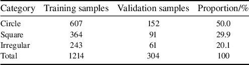
All data for the validation experiments were sourced from laser spot images acquired during the operation of the SG-II facility from 2024 to 2025. The dataset comprises 1214 training images and 304 validation images, encompassing three typical spot morphologies: ‘circle’, ‘square’ and ‘irregular’.

These three morphologies coexist simultaneously during facility operation and correspond to spot patterns at different optical path positions. Specifically, the circular spot is the near-field morphology of the rod amplifier before main amplification injection, the square spot is the near-field morphology at the main amplification output and the irregular spot is the far-field morphology at the main amplification output.

Standard examples of these three categories are shown in Figure 9. All images were uniformly resized to 800×800 pixels during preprocessing. Pixel-level annotation was performed using the LabelMe tool and subsequently converted to the YOLO format.

Figure 9

Examples of three types of laser spots: (a) circle; (b) square; (c) irregular.

While the dataset size (1214 training + 304 validation images) is modest for deep learning, strong pre-training on the COCO database and data augmentation effectively mitigate overfitting risks. Three independent runs show stable performance, indicating good generalization.

The detailed category distribution of the dataset is presented in Table 2. It can be observed that the ‘circle’ category constitutes approximately 50% of the dataset, which aligns with the most common physical characteristic of far-field spots in the actual operation of the SG-II facility.

Table 2

Distribution of the laser spot dataset.

Table 2 Long description

The table consists of four columns: Category, Training samples, Validation samples, and Proportion/percent.

* Row 1: Circle category contains 607 training samples and 152 validation samples, accounting for 50.0 percent of the dataset.

* Row 2: Square category contains 364 training samples and 91 validation samples, accounting for 29.9 percent of the dataset.

* Row 3: Irregular category contains 243 training samples and 61 validation samples, accounting for 20.1 percent of the dataset.

* Row 4: Total values are 1214 training samples and 304 validation samples, totaling 100 percent.

The dataset is mainly derived from normal SG-II facility alignment scenarios, with approximately 20% low signal-to-noise ratio (SNR) (<15 dB) samples included, while systematic coverage of extreme anomalies (beam missing, strong saturation, severe misalignment, out-of-reference spots) is limited due to their extremely low occurrence frequency and insufficient annotated samples. For real-time alignment, a graceful degradation mechanism is adopted: the system raises detection failure flags for abnormal cases instead of outputting erroneous estimates, triggering manual intervention to ensure operational safety.

3.1.2 Experimental environment

The experiments were conducted on a computer running the Windows 11 operating system. The hardware configuration included an Intel Core i9-14900HX processor (with a base frequency of 2.20 GHz) and an NVIDIA GeForce RTX 4060 Laptop GPU (with 16 GB of VRAM). The software environment consisted of Python 3.13, PyTorch 2.8.0 and CUDA 12.9. The training was implemented based on the Ultralytics YOLOv8 framework.

3.3.1 Impact of backbone network improvements

Progressive ablation experiments demonstrate that the baseline YOLOv8-seg model achieves a baseline mAP@0.5 performance of 0.872 ± 0.003. The introduction of the CBAM module increases this score to 0.891 ± 0.002, an improvement of 2.18%, validating its effectiveness in extracting features from low-contrast spots. Although the dynamic multi-scale fusion strategy causes a slight overall decrease in mAP@0.5 to 0.885 ± 0.004, it increases the recall rate for the irregular category by 4.1%, indicating enhanced adaptability to deformed targets. The circularity constraint loss function raises the average circularity of circle-type spots from 0.832 to 0.896.

The full model, integrating all improvements, achieves an mAP@0.5 of 0.901±0.002, representing a 3.33% improvement over the baseline, with only a 10 ms increase in inference time. It maintains real-time processing capability at 55 ms per frame on an RTX 4060 GPU. The detailed results are listed in Table 3.

Table 3

Results of ablation experiments on backbone network improvements (network component analysis) ^a .

Table 3 Long description

The table consists of five columns: Model configuration, m A P at 0.5, m A P at 0.5 to 0.95, Inference time in milliseconds, and Training G P U memory in G B.

* Y O L O v 8-seg baseline: m A P at 0.5 is 0.872 plus or minus 0.003. m A P at 0.5 to 0.95 is 0.756 plus or minus 0.004. Inference time is 45 plus or minus 1. G P U memory is 8.7 plus or minus 0.2.

* Plus C B A M attention: m A P at 0.5 is 0.891 plus or minus 0.002. m A P at 0.5 to 0.95 is 0.774 plus or minus 0.003. Inference time is 48 plus or minus 1. G P U memory is 8.9 plus or minus 0.2.

* Plus Dynamic multi-scale fusion: m A P at 0.5 is 0.885 plus or minus 0.004. m A P at 0.5 to 0.95 is 0.781 plus or minus 0.002. Inference time is 52 plus or minus 1. G P U memory is 9.1 plus or minus 0.2.

* Plus Circle constraint loss: m A P at 0.5 is 0.888 plus or minus 0.003. m A P at 0.5 to 0.95 is 0.771 plus or minus 0.005. Inference time is 47 plus or minus 1. G P U memory is 8.8 plus or minus 0.2.

* Full model: m A P at 0.5 is 0.901 plus or minus 0.002. m A P at 0.5 to 0.95 is 0.788 plus or minus 0.003. Inference time is 55 plus or minus 2. G P U memory is 9.2 plus or minus 0.2.

Asterisks indicate statistically significant improvements over the baseline with p less than 0.01 for single asterisk and p less than 0.005 for double asterisks.

^a The term ‘ablation experiments’ here refers to network component validation in machine learning, not the physical process of laser ablation.

* and ** indicate statistically significant improvement compared to baseline (*p < 0.01, **p < 0.005).

Table 4

Per-class performance metrics.

Table 4 Long description

The table consists of six columns: Class, A P @ 0.5, A P @ 0.5 to 0.95, Precision, Recall, and F 1.

* Circle: A P @ 0.5 is 0.912, A P @ 0.5 to 0.95 is 0.798, Precision is 0.926, Recall is 0.908, and F 1 is 0.917.

* Square: A P @ 0.5 is 0.898, A P @ 0.5 to 0.95 is 0.782, Precision is 0.918, Recall is 0.918, and F 1 is 0.918.

* Irregular: A P @ 0.5 is 0.893, A P @ 0.5 to 0.95 is 0.784, Precision is 0.872, Recall is 0.901, and F 1 is 0.886.

* Mean: A P @ 0.5 is 0.901, A P @ 0.5 to 0.95 is 0.788, Precision is 0.905, Recall is 0.909, and F 1 is 0.907.

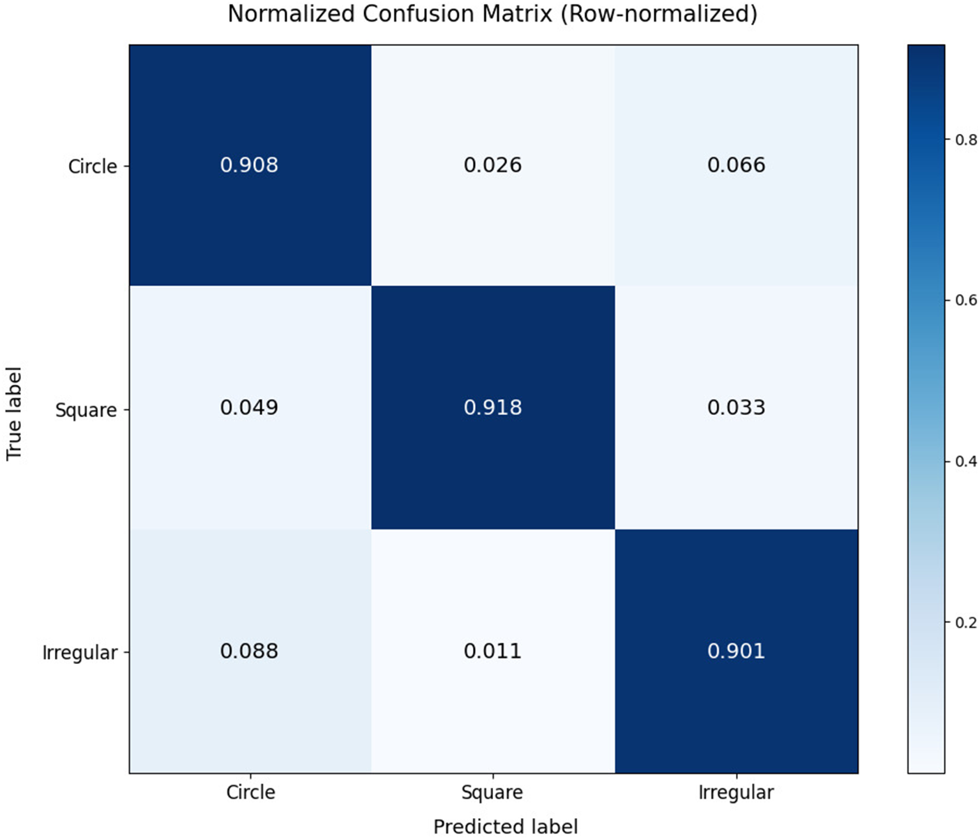
To further analyze the model’s performance across different spot types, we present the confusion matrix and per-class metrics in Figure 10. The results demonstrate that the model achieves consistent performance across all three categories.

Figure 10

Confusion matrix for three spot types at the IoU threshold of 0.5.

Figure 10 Long description

The heatmap displays a three by three grid with Truth labels on the vertical y-axis and Predict labels on the horizontal x-axis. Both axes list Circle, Square, and Irregular. A color scale bar on the right indicates values from 0.0 to 0.8 in shades of blue.

* The first row for Truth label Circle shows values of 0.908 for Circle, 0.026 for Square, and 0.066 for Irregular.

* The second row for Truth label Square shows values of 0.049 for Circle, 0.918 for Square, and 0.033 for Irregular.

* The third row for Truth label Irregular shows values of 0.088 for Circle, 0.011 for Square, and 0.901 for Irregular.

The diagonal cells from top-left to bottom-right represent correct predictions and are colored dark blue, indicating high accuracy above 0.9 for all categories.

The model achieves consistent and competitive detection performance across all three spot categories, with a mean AP@0.5 of 0.901. Notably, the circle class achieves the highest AP@0.5 (0.912), with a precision of 0.926 and recall of 0.908, benefiting from its distinct circular shape and abundant training samples (50% of the dataset). The irregular class, despite having the smallest sample size (20% of the dataset), maintains excellent performance with an AP@0.5 of 0.893 and the highest F1-score of 0.918, demonstrating the model’s outstanding robustness to shape variations. The square class also delivers balanced detection capability with a high recall of 0.901, ensuring reliable and low-miss-rate detection in practical laser alignment scenarios, as shown in Table 4.

3.3.2 Impact of post-processing optimization on contour quality

The post-processing module takes the raw segmentation mask as input and sequentially performs morphological filtering and shape constraint optimization. Without post-processing, the radius error for circle-type spots was 2.35 ± 0.15 pixels, and the circularity error was 0.068 ± 0.008. After introducing the morphological filtering layer (with a 1×1 opening kernel and a 4×4 closing kernel), the radius error decreased to 2.01 ± 0.11 pixels (an improvement of 14.5%, p < 0.01), the circularity error decreased to 0.051 ± 0.006, and the processing time increased by 3 ms. Upon adding the circularity constraint layer (which blends the predicted mask with an ideal circle in a 3:7 weight ratio), the radius error was further reduced to 1.92 ± 0.09 pixels (a cumulative improvement of 18.3%, p < 0.01) and the circularity error decreased to 0.041 ± 0.005, with a total processing time increase of 8 ms. The effects of post-processing optimization are summarized in Table 5.

Table 5

Summary of post-processing optimization effects ^a .

Table 5 Long description

The table consists of four columns: Post-processing configuration, Radius error forward slash pixel, Circularity error, and Processing time forward slash m s.

Row 1: No post-processing. Radius error is 2.35 plus or minus 0.15. Circularity error is 0.068 plus or minus 0.008. Processing time is the Baseline.

Row 2: plus Morphological filtering. Radius error is 2.01 plus or minus 0.11. Circularity error is 0.051 plus or minus 0.006. Processing time is plus 3.

Row 3: plus Circle constraint. Radius error is 1.92 plus or minus 0.09 asterisk. Circularity error is 0.041 plus or minus 0.005 asterisk. Processing time is plus 5.

Row 4: Complete post-processing. Radius error is 1.92 plus or minus 0.09 asterisk. Circularity error is 0.041 plus or minus 0.005 asterisk. Processing time is plus 8.

Notes: asterisk indicates statistically significant improvement where p is less than 0.01.

^a * indicates statistically significant improvement (p < 0.01).

3.3.3 Training dynamics analysis and performance evaluation

This study provides a detailed analysis of the model’s performance throughout the training process, with a specific focus on the evolution of the segmentation loss and the mAP.

Figure 11 illustrates the variation of the segmentation loss during training and validation. After a brief peak at epoch 56, the segmentation loss continued to decline, indicating stable learning convergence. The brief validation loss peak at epoch 56 coincides with the transition from learning rate warm-up to cosine annealing schedule. This transient instability quickly resolves as the optimizer adapts to the new learning rate regime, demonstrating good training robustness.

Figure 11

Segmentation loss trend.

Figure 11 Long description

The x-axis is labeled Epoch and ranges from 0 to 140. The y-axis is labeled Loss and ranges from 0 to 4. A legend in the top right identifies two lines. Train seg loss in dark blue and Val seg loss in yellow.

* The Train seg loss line begins at approximately 1.3 and follows a steady asymptotic decay, decreasing smoothly to approximately 0.5 by epoch 140.

* The Val seg loss line begins much higher at approximately 4.7. It drops sharply within the first 5 epochs to around 1.6, then exhibits significant volatility between epochs 5 and 40.

* A prominent vertical spike occurs in the Val seg loss at approximately epoch 55, reaching a loss value of 2.7 before immediately returning to the baseline trend.

* After epoch 60, the Val seg loss stabilizes with minor fluctuations, maintaining a consistent gap above the training loss and ending at approximately 0.8.

Figure 12 shows the progression of the segmentation mAP metrics across training epochs. It can be observed that both mAP@0.5 and mAP@0.5:0.95 increased rapidly during the initial phase before stabilizing. The final mAP@0.5 approached 0.9, while mAP@0.5:0.95 stabilized around 0.75, demonstrating a steady improvement in segmentation performance.

Figure 12

Segmentation mAP metrics trend.

Figure 12 Long description

The X-axis is labeled Epoch and ranges from 0 to 140. The Y-axis is labeled m A P and ranges from 0.1 to 0.9. Two lines are plotted.

* The top line, colored yellow, represents m A P at 0.5. It shows a rapid logarithmic increase from 0.1 to approximately 0.75 within the first 10 epochs. It then continues a jagged upward trend, fluctuating between 0.8 and 0.9 for the remainder of the training. A significant sharp downward spike occurs near epoch 55 before immediately recovering.

* The bottom line, colored dark red, represents m A P at 0.5 colon 0.95. It follows a similar trajectory but at a lower intensity, rising quickly to 0.6 by epoch 10 and then stabilizing into a slow, jagged climb that plateaus around 0.75. It also exhibits the same sharp downward spike at epoch 55.

A legend in the bottom right corner identifies the yellow line as m A P at 0.5 and the dark red line as m A P at 0.5 colon 0.95.

The loss variation curve indicates that the model can stably learn effective feature representations from the data. As training progresses, the loss value continuously decreases, reflecting a gradual improvement in the model’s fit to the training samples and a corresponding reduction in prediction error. The transient peak in the mid-training phase is attributed to the learning rate strategy transition, rather than model overfitting or dataset bias. The model quickly recovers and continues to optimize thereafter, further validating its excellent training stability and robustness. Concurrently, the mAP metrics show a steady upward trend, with a particularly noticeable improvement during the initial training stage, indicating that the model’s segmentation performance is substantively enhanced as training proceeds. Overall, the proposed model exhibits stable convergence characteristics and continuous performance improvement throughout the training process, and converges stably to high performance, providing a reliable foundation for its further optimization and practical deployment.