1 Uniformitarianism

Uniformitarianism allows us to explain the past in terms of what we know about the present. The limitations of this practice are obvious and all historical disciplines struggle with them (see also Lass Reference Lass1997: 24–32). Problems are most acute when dealing with phenomena that are culturally mediated, immaterial or both. As it happens, the immaterial and culturally mediated is also the domain to which much of the subject matter of historical linguistics belongs. And indeed, while uniformitarianism is generally accepted in linguistics as a useful principle, related to the more general principle known as Ockham's razor (see Janda & Joseph Reference Janda and Joseph2003: 25), it has obvious limitations in this field as well (see also Bergs Reference Bergs, Hernández-Campoy and Conde-Silvestre2012). For example, detailed sociolinguistic work may reveal how languages change in a speech community, but it would be ill-advised to project the findings from studies about twenty-first-century city-dwellers to pre-industrialized speech communities. Reviewing a number of twentieth-century changes, Labov (Reference Labov2001b: 279–84) points out that in the majority of cases women initiate a change, and men adopt it later. But many a linguist, including Labov himself (see Reference Labov2001a: 23), would be hesitant to claim this would have been necessarily true in mediaeval or Palaeolithic communities as well (but see Blaxter Reference Blaxter2015, who ventures to answer the question).

This turns historical research into something of a balancing act. Without uniformitarianism, one feels no real understanding is achievable. If events from the past are really governed by their own laws we cannot fully understand them, as these laws cannot be tested in a controlled research setting today. At the same time, our interest in studying the past lies precisely in the fact that the past was different. When we put our faith in uniformitarianism we assume that at some level of abstraction the difference dissolves. However, because we do not know exactly when that happens, we always run the risk of underestimating just how different the past really was. Not enough uniformitarianism, and we fall short of explaining anything – too much of it, and we inadvertently reduce the past to a bleached version of the present. Labov calls this ‘The Historical Paradox’. ‘The task of the historical linguist is to explain the differences between the past and the present; but to the extent that the past was different from the present, there is no way of knowing how different it was’ (Labov Reference Labov2001a: 21).

Of course, any discipline faces uncertainty. If historical disciplines are more preoccupied with this uncertainty, it is perhaps because falsification tends to be more difficult. The past cannot be interrogated as the present can. Most of the evidence one might rely on has been irretrievably lost. Whatever sources of evidence are left are finite and partial. We may be told that the syntax of the language spoken by Homo sapiens 40,000 years ago was essentially similar to the syntax of contemporary human language (Hauser et al. Reference Hauser, Chomsky and Tecumseh Fitch2002) or that þam cynge licodon peran, though unattested, was an acceptable Old English sentence (Jespersen Reference Jespersen1927: 208–9). But we cannot check this the way we might check similar claims about linguistic universals or about the grammar of Present-day English.

Still, there are things to keep the historical linguist from despair. First, the difference in available evidence is not an absolute one but one of degree. Some historical sources are so abundant that they are for many practical purposes inexhaustible. Second, technological advances may make it possible to investigate old data sources in new ways. Third, the historical disciplines have something that is unique and envied by all the others: real-time data. If we really want to know whether theories based on synchronic evidence have universal application, we have to confront real-time data. In this spirit, the case study we present in this article reflects some of the possibilities but also some of the frustrations that come with such data when used to test a uniformitarian claim about one immaterial aspect of language: linguistic structure.

2 Degrees of structure

Linguists generally agree that underlying structure exists, but disagree on its nature and on how to represent it. At one extreme, structure is set down in stable rules that exist independently of the forms over which they operate (e.g. Chomsky Reference Chomsky1981). At the other, structure is emergent from the very things it structures and is, consequently, in constant flux (e.g. Hopper Reference Hopper and Tannen1988).

The debate on the nature of structure turns up in different guises. In morphology, derived words like sluggish or disorganize are structured, as they consist of recognizable units with a fixed form and meaning – traditionally known as morphemes – that have been put together in a recognizable way. The difference with non-derived words like yellow or aubergine seems straightforward. But it is not (Aronoff Reference Aronoff1976). One problem is forms of which the one part looks like a legitimate morpheme but the other fails to recur in any other combination. Arid – fluid – languid – livid – solid – squalid are all adjectives sharing the form id but they have no recognizable base. In flap – flare – flash – flick – flinch – flip – flit – flop – fluke – flump the recurrent form fl- even seems to come with a recurrent meaning – ‘short and sudden movement’. And in hapless – reckless – ruthless the -less is in fact a known suffix, as in witness – aimless – faceless – fearless – priceless – senseless – sleepless etc. – but again the base is not. Another problem is that potential morphemes show variation in their form or meaning. Does the form /iːz/ in disease and easy make one morpheme, even though its meaning is not constant? And do the words nosy and nasal share a single (abstract) form /nVz/ meaning ‘nose’? The simplest decision is to say that most or all of these problematic words are non-complex, since they could not have been coined by a morphological rule. Nevertheless, it is tempting to assign some degree of structure.

By now, different types of independent evidence have been advanced to support gradient structure in morphology (Hay & Baayen Reference Hay and Harald Baayen2005; Blumenthal-Dormé Reference Blumenthal-Dormé2012). Hay (Reference Hay2003), for instance, demonstrates that when speakers are asked to discriminate between the more complex and the less complex form in pairs like settlement – government, they can do so with high consistency – typically, settlement is chosen as the more complex form. In a very different kind of study, Gonnerman et al. (Reference Gonnerman, Seidenberg and Andersen2007) use lexical decision tasks to study the magnitude of priming effects between derived forms and their bases. They demonstrate that priming effects vary in magnitude. For instance, boldly primes bold more strongly than lately primes late.

Findings like these support the idea that structure is gradient, in that some complex words are more readily decomposable into base and affix than others – a property we will refer to here as ‘analysability’. Analysability refers to the degree to which language users can recognize the individual parts of a composite whole (Langacker Reference Langacker1987: 448; Bybee Reference Bybee2010: 45). Analysability is closely related to compositionality, which refers to the degree to which the properties of a composite whole are predictable from the properties of its parts (Langacker Reference Langacker1987: 448; Bybee Reference Bybee2010: 45). Analysability is the broader term, however, in that an expression may decrease in analysability without losing compositionality, but not vice versa. In addition, while an expression's compositionality is a function of its semantic and formal characteristics, its analysability is an underlying property that is not directly accessible to the observer.

Importantly, both Hay (Reference Hay2003) and Gonnerman et al. (Reference Gonnerman, Seidenberg and Andersen2007) are able to make predictions as to which words are likely to be more analysable. Hay (Reference Hay2003) argues that phonotactics and the relative frequency of base and derivation play a role. For instance, government is less analysable than settlement because the derived form government is more frequent than its base govern, while the derived form settlement is less frequent than its base settle. Gonnerman et al. (Reference Gonnerman, Seidenberg and Andersen2007) show that other important determinants are the degree of semantic and formal similarity between a base and the corresponding free form. For instance, lately is less compositional – and hence less analysable – than boldly because the semantic contribution of late to lately is less predictable than that of bold to boldly.

Gradience also crops up in historical linguistics. One challenge is presented by grammaticalization processes (Traugott & Trousdale Reference Traugott and Trousdale2010). For instance, grammaticalization is often accompanied by formal reduction. This may result in a formal continuum between the reduced form and the original full form. Krug (Reference Krug2000: 152), for instance, cites the forms [ˈwɒntˌtʰuː], [ˈwɒntˌtʊ], [ˈwɒntʊ], [ˈwɒntə], [ˈwɒnə], [ˈwənə], [wɒn] and [wã] as potential realizations of English want to. Grammaticalization also comes with semantic changes which may likewise be gradual. For example, Dutch zitten developed from a posture verb with accompanying purpose adjunct, literally meaning ‘sit down to do something’, into an aspectual construction, marking duration or repetition. The development is reflected in a synchronic gradient. In present-day usage, the posture sense of zitten may be clearly present as in (1a), vaguely present as in (1b), or absent as in (1c) (Lemmens Reference Lemmens2005).

1. (1)

   1. (a) kijk als ik hier ’s avonds zo effe zit te lezen of TV zit te kijken joh dan hoor ik ze lachen of weet ik veel wat maar da ’s niet erg (Corpus Gesproken Nederlands (CGN))

      ‘look, when I'm just sitting here in the evening reading or watching the telly, well, I can hear them laughing or whatever but that doesn't matter’

   2. (b) warm ja [. . .] maar niet te veel in de zin van dat je zit te te barbecuen in je huis (CGN)

      ‘warm, yes, but not too warm in the sense that you're being roasted in your own house (lit. sit being roasted)’

   3. (c) ik weet altijd hoe dat bij ons gaat |Arnold komt als laatste uit z'n bed |m'n moeder zit te stressen op Arnold van Arnold schiet nou toch ’ns op (CGN)

      ‘I know how this always goes in our place. Arnold is the last to get out of bed. My mother is going at Arnold like Arnold, get a move on. (lit. sits going at him)’

As in morphology, the question is whether these formal and semantic continua reflect gradience at the structural level. Traditionally, underlying syntactic change has been seen as abrupt (e.g. Harris 2003). However, there are dissenting views. One line of reasoning links grammaticalization to structural gradience through frequency (Haspelmath Reference Haspelmath1999; Bybee Reference Bybee2003, Reference Bybee2006, Reference Bybee2010). Grammaticalizing forms become more frequent. This makes it more likely that they are stored autonomously. As a result, they become dissociated from their component parts. This licenses semantic and formal change, which in turn contributes to the dissociation between the whole and its parts. The gradient, then, is fundamentally one of analysability. In principle, this idea can be tested experimentally, at least on synchronic data. For example, Vogel Sosa & MacFarlane (Reference Vogel Sosa and MacFarlane2002) instructed English-speaking participants to press a key on a keyboard as soon as they heard the word of in a stretch of natural speech. They found that reaction times to of were slower in high-frequency collocations, such as out of, sort of or some of, than in less frequent collocations, such as because of, each of or sense of. According to them, this indicates ‘holistic storage for the frequent collocations and therefore impeded access to of as an independent word’ (Vogel Sosa & MacFarlane Reference Vogel Sosa and MacFarlane2002: 233–4).

In diachrony, it is much harder to test the idea of gradually changing analysability. But there may be a way out. In a study reminiscent of the priming experiments by Gonnerman et al. (Reference Gonnerman, Seidenberg and Andersen2007), Torres Cacoullos (Reference Torres Cacoullos, Adli, García and Kaufmann2015) uses written historical data to show that the Spanish progressive construction, consisting of estar and a gerund, appeared to be initially primed by any other use of the verb estar, but the priming relation became weaker with time as the construction grammaticalized. Torres Cacoullos explicitly invokes ‘priming effects as a measure of (erosion of) analyzability’ (Reference Torres Cacoullos, Adli, García and Kaufmann2015: 266). Accordingly, she interprets the evidence as suggesting a gradual dissociation between estar in general and its specialized use in the progressive construction:

Torres Cacoullos's study offers a promising method to test whether underlying structures can become gradually less analysable over time. Crucially, it also shows that priming effects can be studied and exploited to make a theoretical point even in historical written data (see also Rosemeyer & Schwenter Reference Rosemeyer and Schwenter2017).

The goal of this article is similar to that of Torres Cacoullos (Reference Torres Cacoullos, Adli, García and Kaufmann2015), viz. to catch in action the changes that alter the underlying structure of complex forms. In what follows we address changes in the degree of analysability of English ly-adverbs. These are adverbs formed from adjectives by the addition of the suffix ly, such as cheaply, categorically, specially or morally. It is expected that ly-adverbs may vary in analysability – i.e. the degree to which ly-adverbs are recognized as consisting of an adjectival base and the ly-suffix. Further, it is expected that analysability may change over time, subject to frequency changes, whether they are changes in the token frequency of an individual adverb (cf. Gordon & Alegre Reference Gordon and Alegre1999; Bybee Reference Bybee2006) or in the relation between the frequency of the adverb and that of its base (see Hay Reference Hay2003; Blumenthal-Dormé Reference Blumenthal-Dormé2012).

To test these expectations, we adopt a method similar to that of Torres Cacoullos (Reference Torres Cacoullos, Adli, García and Kaufmann2015), based on the assumption that historical data can reveal priming effects and that the presence or absence of such effects says something about a form's underlying properties. A form whose underlying structure is less analysable will be less likely to prime or to be primed by other forms with a similar structure. We assume that priming effects hold between a prime and a target if the occurrence of the prime positively affects the likelihood of subsequent occurrence of the target. While such effects may be slight, they should occur in spontaneous production data, meaning that they should be observable in a big enough corpus.

Our study differs from that by Torres Cacoullos in two important ways, both having to do with the choice of case study. First, our case study should allow us better to isolate structural priming effects (Bock Reference Bock1987). We can take the more abstract derivational template [Adjective + ly] as prime and see how its occurrence affects the likelihood of occurrence for any specific ly-adverb. This way, the magnitude of the observed priming effects primarily reflects a structural property of the ly-adverb in question. Second, the effect of underlying structural change can be tested on a much larger number of individual cases – in principle, any ly-adverb that occurs in more than one subperiod of the corpus. This potential for systematic replication should make findings much more reliable. We should avoid being misled by a lucky find, and we should also get some idea of the overall magnitude of the effects we are interested in.

As data source we used the Hansard Corpus (HC), which consists of transcripts of Parliamentary debates in the British Houses of Parliament from 1803 to 2005. The HC can be consulted online at www.hansard-corpus.org, but we used an offline version provided by Marc Alexander of the University of Glasgow. The HC has the advantages of being very large (1.6 billion words in total) and of coming as close to spoken language use as historical corpora get (needless to say, though, it is still a good way removed from having accurate transcriptions of spontaneous conversation). In the following sections, we will first explain the method we used to identify priming effects in this data source (section 3). Next, the method is tested by doing a synchronic study on one slice of the corpus, namely the 1990s (section 4). After that, we turn to actual change by extending the method to the period from 1950 to 2005 (section 5). We then return to the issue of uniformitarianism in historical linguistics by briefly discussing the possibilities of and limitations to historical data (section 6). Finally, we comment on Martin Hilpert's response to our study in this volume (section 7).

3 Measuring priming effects in corpus data

Priming studies on corpus data typically adopt a variationist framework, examining whether one alternate of a pair of alternates is chosen more often when it has been primed in the previous discourse (Weiner & Labov Reference Weiner and Labov1983; Gries Reference Gries2005; Szmrecsanyi Reference Szmrecsanyi2006). Because the great majority of ly-adverbs cannot be construed as members of an alternating pair we take a different approach here.

There are two potentially relevant measures. First, the more analysable a specific ly-adverb is, the more sensitive it will be to priming by other ly-adverbs. We call this relation ‘passive priming’ because the adverb in question is being structurally primed. In corpus data passive priming will translate into a tendency for the adverb to occur in the vicinity of other ly-adverbs that occurred earlier in the discourse and functioned as prime. In other words, the context immediately preceding our adverb will tend to have slightly more ly-adverbs than one would normally expect. Second, it can be expected that a highly analysable ly-adverb will be more capable of structurally priming other ly-adverbs. This is ‘active priming’ because the adverb in question structurally primes other adverbs. In corpus data active priming should translate as a slightly higher than expected incidence of ly-adverbs immediately following the priming adverb. Of course, these frequency differences offer only a proxy to priming, but then so do the reaction times in psycholinguistic experiments.

To make this more concrete, consider example (2), which is a typical instance of permanently from the 1990s section of the HC. Permanently is preceded by a left context (marked LC), specified here as a 500-character window to its left. Similarly, it has a right context (marked RC), specified as a 500-character window to its right. The left context consists of 97 words including 3 other adverbs – periodically, viciously and obviously. We can normalize this and say that in (2) adverbs occur 3.093 times per hundred words (=3/97*100). The right context has 86 words of which one is an additional adverb – immediately. So here other adverbs occur at 1.163 adverbs per hundred words (=1/86*100). Knowing that throughout the 1990s section of the HC, ly-adverbs occur with a frequency of 1.081 per hundred words, the left context in (2) can be said to have more adverbs than expected, while the right context approximates the expected number.

1. (2) [pit bull terriers and other dogs: We are periodically reminded of this situation by the press: Even today there is a newspaper report about a pit bull terrier viciously attacking another dog: The intent of the legislation was obviously to protect the public from such attacks: A welcome corollary to that was that it might assist in the prevention of the awful sport of dog fighting or dog baiting: In the long run, it was a humane path to eliminate from Britain dogs of the pit bull terrier type by requiring that such dogs be registered, neutered,]_LC permanently [identified, muzzled and kept on a leash in public: If any of those conditions was contravened the dog would be seized and destroyed and the owner prosecuted: Several months ago an example of that could be found in the newspapers: A dog had its muzzle removed for a minute or so, in order to quench its thirst and was immediately seized: That dog is now under threat of destruction for that misdemeanour: The noble Lord, Lord Houghton, has addressed in particular the question of what one]_RC (1993, HC)

By itself, example (2) is of course unconvincing, but if all 1,589 instances of permanently in the 1990s section of the HC are taken into account, all with their left and right contexts, we arrive at more revealing figures. It turns out that in the contexts to the left of permanently other ly-adverbs occur with a frequency of 1.322 per hundred words. That is more than expected, with an observed-to-expected ratio of 1.22 (meaning we have about 22 per cent more chance of finding an adverb in the contexts to the left of permanently than we do on average in the corpus as a whole). In the contexts to the right of permanently, the frequency of other ly-adverbs is 1.275 per hundred words – again more than expected, with an observed-to-expected ratio of 1.18.

We assume that these findings can be interpreted in terms of priming. That is, permanently is being structurally primed by the adverbs in its left context (passive priming) and is itself responsible for priming other adverbs in its right context (active priming). If that assumption is correct, the observed-to-expected ratios provide a measure of the strength of this priming effect. Indirectly, we then also have a measure of the analysability of permanently: if permanently structurally primes or is primed by other ly-adverbs, its own underlying structure must be recognizable.

4 Validation on synchronic material

To see whether the proposed method can say anything about morphological analysability, we applied it to the 250 most frequent ly-adverbs in the 1990s section of the HC. The relevant information was collected from the corpus automatically, using a Perl-script written for the purpose. The left and right contexts for any given adverb were defined as 500-character strings to the immediate left and right of the adverb in question (which corresponds to approximately one hundred words), bounded by the beginning and ending of a speaker turn. Frequency counts for ly-adverbs were conducted excluding the most frequent false matches (e.g. friendly, Italy, supply) and also always excluding the target adverb itself. Recall that adverbs that are more analysable should come with stronger priming effects. For the synchronic analysis, results for passive and active priming are well correlated (Pearson correlation = 0.73, p < 0.001). In the discussion we focus on passive priming effects only.

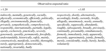
Table 1 shows the adverbs that are most and least sensitive to passive priming, as based on the observed-to-expected ratios for the frequency of ly-adverbs in the context preceding the adverbs (see section 3 above). The left-hand side of the table lists the adverbs that are highly sensitive to passive priming (with an observed-to-expected ratio above 1.20), while the right-hand side lists the adverbs that are only weakly sensitive to passive priming (with an observed-to-expected ratio below 1.05).

Table 1.

Adverbs with high and low sensitivity to passive priming

The results in table 1 are encouraging. Its right-hand half contains some of the adverbs one would reasonably expect to have low analysability. These include hardly, which Gonnerman et al.’s (Reference Gonnerman, Seidenberg and Andersen2007) test subjects found to have little semantic overlap with its base adjective hard. They also include some adverbs that have very infrequent adjectival bases, such as presumably (whose base presumable is attested only once in the 1990s section of the HC). Moreover, many of the adverbs in the right-hand half of table 1 typically serve as function words, such as the degree modifiers merely, really and barely, the focusing adverb specifically, the approximators nearly roughly and approximately, the evidential adverbs apparently and allegedly, or the disjuncts alternatively and briefly. In contrast, the left-hand half of table 1, while also having some function words, such as mainly, contains many more items that are content-words and which one would typically find functioning as VP-adverbs, such as efficiently, genetically, generously, speedily or safely.

To further test how well our method performs we checked whether the items that our priming-based approach identified as being low in analysability would be predictable from the parameters generally assumed to affect analysability. One often-quoted determinant is simple frequency (Bybee Reference Bybee2006). In addition, the synchronic research by Hay (Reference Hay2001, Reference Hay2003) indicates that analysability is lower in morphologically derived forms whose frequency is relatively high compared to the frequency of their base. In her study, Blumenthal-Dormé compares the effects of simple token frequency and adverb/base ratio, finding that only adverb/base ratio has a significant effect on analysability (Reference Giegerich2012: 150, 191). However, Bybee (Reference Bybee2010: 46–7) suggests that simple token frequency effects might still kick in in the higher-frequency ranges. Further, it should be pointed out that, just as in Hay's (Reference Hay2001, Reference Hay2003) work, Blumenthal-Dormé’s focus is exclusively on derivational morphology, where holistic representation of complex forms is probably the default (Reference Giegerich2012: 201). It is not unreasonable to assume that inflectional morphology works differently (irrespective of whether inflection and derivation represent radically distinct processes or are just two extremes on a continuum). Studies on inflectional morphology do suggest simple token frequency effects in at least some cases (Gordon & Allegre Reference Gordon and Alegre1999; Ford et al. Reference Ford, Marslen-Wilson, Davis, Baayen and Schreuder2003). With English ly-suffixation sitting on the border between inflection and derivation, as reflected in the theoretical debate concerning its status (Giegerich Reference Giegerich2012), the most reasonable procedure here is to start out agnostically, and simply put the two different frequency measures to the test.

Next to the two frequency measures, there is one more potentially relevant determinant of analysability that can be derived from the literature and which can be applied to our case study. Hay (Reference Hay2003) argues that an item's analysability tends to be lower if its morpheme boundary is less easily inferred from phonotactic cues. For example, because the phonemes /tl/, which straddle the morpheme boundary in promptly, cannot form a syllable onset nor a coda in English they are very likely to belong to different morphemes. For this reason, the morpheme boundaries in words like promptly, keenly or accordingly are relatively easily identified. In contrast, the morpheme boundaries in words like locally, thoroughly or highly are not given away by phonotactic cues and are less easily identified.Footnote ¹

To test all 250 adverbs at once, the various predictors – frequency, adverb/base ratio and the presence of a phonotactic juncture – were fed into a bidirectional variable selection procedure for a multiple linear regression model, with the measure for passive priming as dependent variable.Footnote ² The independent variables were operationalized as follows:

• • Frequency was operationalized as an adverb's log-transformed normalized frequency in the HC. The variable was centred to arrive at a more sensible interpretation of the intercept.

• • The adverb/base ratio was made into a binary factor, with one level for adverbs that are more frequent than their adjectival base, and the other level for adverbs that are less frequent than their base. Note that some bases are not always used as adjectives – for instance, supposed in supposedly is typically a verb, or commercial in commercially may be used as a noun. In such cases we made no attempt to single out the adjectival uses.

• • The presence of a phonotactic juncture was also operationalized as a binary variable. This is mostly unproblematic but there are some cases that required a special coding decision. In words like formerly a non-rhotic pronunciation was assumed (giving a pronunciation identical to that of formally) – in formerly, therefore, there is no phonotactic juncture, since /əl/ is a possible rhyme in English, contrary to rhotic /ərl/. In words like poorly the vowel quality would give away the syllable boundary even on a non-rhotic pronunciation – in poorly, therefore, there is a phonotactic juncture, since /ʊəl/ is not a possible rhyme. In words like terribly, /bl/ is not a possible coda but because it is a possible onset the morpheme boundary is still obscured, which is why such words were scored as having no phonotactic juncture.

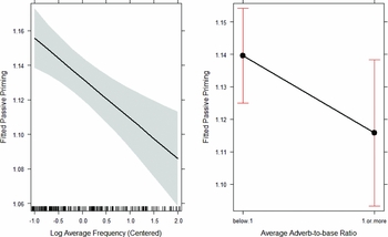
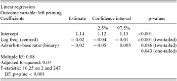
The variable selection procedure was based on the Akaike Information Criterion (AIC), seeking a balance between the goodness of fit and complexity of competing models. The lowest AIC is reached for a model that includes frequency and adverb-to-base ratio, but without the phonotactic juncture variable. In this model, the two explanatory variables support the hypothesis that higher frequency and a higher adverb-to-base ratio lead to lower passive priming: the estimates of both predictors have negative signs (see the regression output table 1 and the effect plot in figure 1).

Figure 1.

Synchronic linear regression effect plots

Remarkably, brute frequency works better than the more sensitive adverb-to-base ratio.Footnote ³ The binary adverb-to-base ratio has a significant marginal effect (p = 0.014, two-tailed), and a significant partial effect if we use a one-tailed test (see table 2), which is less convincing than the reassuringly low p-value for the partial effect of frequency (p < 0.001, two-tailed). As the one-tailed test picks up a signal, and as the two variables do not seem to be collinear (Variance inflation factors (vifs) scores are well under 4), we eventually decided to keep both variables in the model. As is clear from the regression output in table 1, the model as a whole is significant (p < 0.001).

Table 2.

Synchronic linear regression output

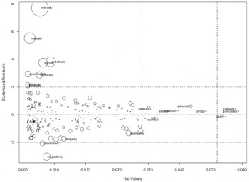
While the above results are promising, it has to be acknowledged that the model has a very modest adjusted R² of 0.07. Further, we checked regression assumptions (Levshina Reference Levshina2015: 155–62). The model displays heteroscedasticity (Non-constant Variance Score Test Chisquare = 41.46, Df = 1, p < 0.001), with larger variance in the higher fitted values, and non-normally distributed residuals (Shapiro-Wilk normality test, W = 0.83, p-value < 0.001). Finally, looking at the Influence Plot in figure 2, we can see that adverbs with high studentized residuals (on the y-axis) are often so-called ‘domain adverbs’ (see Ramat & Ricca Reference Ramat, Ricca and van der Auwera1998: 191 for this term). One reason might be that these adverbs often come in contrastive sequences, as in (3), which could artificially inflate our priming measure.

1. (3) He has cerebral palsy; nevertheless, he is contributing economically, socially and politically to the life of his community. (1990, HC)

Figure 2.

Synchronic linear regression model influence plot

At the other end of the y-axis we find two text-structuring adverbs, alternatively and respectively, that are less subject to passive priming than the model suggests.Footnote ⁴ Fitting the same regression model on the adverbs that have studentized residuals lower than 2 or higher than –2 increases significance and decreases effect size for frequency, and decreases both significance and effect size for adverb-to-base ratio (to the point of insignificance). However, the overall trends, as indicated by the sign of the estimates, remain unaffected.

All in all, it is clear that the model does not adequately capture the entirety of what is driving the passive priming effect. It may be countered that studies on priming using naturalistic (corpus) data are likely to have higher rates of unexplained variance than experimental designs (Gries Reference Gries2005: 386). Moreover, our main concern is not to build a strong, all-encompassing multifactorial predictive model, but rather to establish whether what we assume to be a priming effect reflective of underlying analysability actually behaves as one, in that it responds to known predictors in the expected way. Apart from the missing effect of phonotactic juncture, we found more or less what we expected to find, indicating that our method does what we assumed it would do. Even so, there is no denying that the very large share of unaccounted-for variation in our priming measure is sobering. The unaccounted-for variation may reflect imperfect knowledge as to the complex set of factors that will affect analysability and/or priming. Or it may be that our measure of priming/analysability is simply rather crude. Given that results are still in line with expectations, it is nevertheless worth extending the method to diachronic data.

5 Extension to diachronic material

While the previous section focused on a single synchronic slice of our corpus, our priming measure can in principle be used across the entire corpus. Doing so, we should be able to determine whether an adverb's sensitivity to priming increases or decreases with time, which in turn can point us to changes in its analysability. Such changes in analysability are expected especially when the adverb changes in frequency, or its frequency changes relative to that of its base.

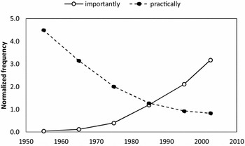
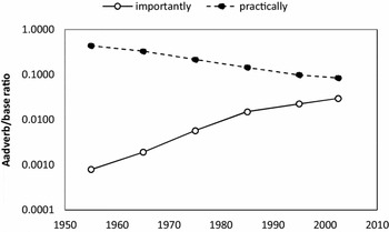
Compare the histories of two adverbs – importantly and practically. Importantly increased in frequency over the period studied. Its adverb/base ratio likewise increased. Practically, on the other hand, decreased in frequency, and so did its adverb/base ratio. This is shown in figures 3 and 4.

Figure 3.

Normalized frequencies of importantly and practically in 1950–2005 (HC)

Figure 4.

Adverb/base ratios for importantly and practically in 1950–2005 (HC)

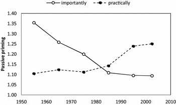
Given the results of our synchronic model (see section 4 above) these developments should go hand in hand with decreasing analysability for importantly and increasing analysability for practically. That is also what is found, as shown in figure 5. In light of this, an item like practically may be said to ‘degrammaticalize’ (Norde Reference Norde2009), as it regains some of its analysability. In fact, this is noticeable also in how practically is used. Based on two random samples of 50 hits, it can be seen that in the 1950s practically is used as a degree modifier, as in (4), in 90 per cent of cases, while its lexical use, illustrated in (5), accounts for only 10 per cent. By the 2000s, the incidence of the lexical use has risen to 30 per cent (the change is significant at p < 0.05, using a Fisher's Exact Test).

1. (4)

   1. (a) The two-year duty had practically no impact in places where the availability of property was so widespread (2001, HC)

   2. (b) Look at Alton Towers, which decided that it would try to take on Battersea power station: That practically killed it (2000, HC)

2. (5)

   1. (a) Surely after 11 September we should see that, practically and tactically, the real and immediate danger is the surreptitiously smuggled weapon (2001, HC)

   2. (b) If money is to be raised, let it be done practically (2001, HC)

Figure 5.

Passive priming for importantly and practically in 1950–2005 (HC)

It is plausible then that the increasing sensitivity to passive priming captures a genuine change in practically, which moves away from structural opacity in the direction of greater analysability.

To be sure, importantly and practically are cherry-picked examples. To more systematically analyse the relation between the changing magnitude of priming effects and changes in the predictors of analysability, we set up a second regression model. The period selected was 1950–2005, which was divided into six subperiods: 1950–9, 1960–9, 1970–9, 1980–9, 1990–9 and 2000–5. We again selected the 250 most frequent adverbs, based on their average frequency across the six periods (note that, being calculated on a different part of the corpus, the set of 250 most frequent adverbs differs somewhat from that in section 4). Next, we calculated the by now familiar measures for active and passive priming, log-transformed normalized frequency and adverb/base ratio. This was done for each of the six periods in the corpus.

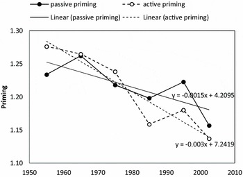
To operationalize change, we took the linear regression slope of each of our measures set out against time (as calculated with respect to the middle of each subperiod). For example, figure 6 shows the priming measures for the adverb permanently over the six subperiods. For permanently, both passive and active priming are on the decline, as appears from the dropping regression lines. Accordingly, the slope of both regression lines, which is expressed by the coefficient of x in the regression formula, is negative. For passive priming the slope is slightly steeper than for active priming, reflected in a more extreme value for the slope coefficient (–0.003 vs –0.0015). Indeed, the slope coefficient can be read as the average annual increase for a given measure for a given adverb, as estimated from the six subperiods in the corpus. As such, the slope coefficient gives us an idea of both the direction and the magnitude of diachronic change.

Figure 6.

Passive and active priming for permanently in 1950–2005 (HC)

The slope coefficient will inevitably be a fairly rough measure, as it is calculated on a mere six measurement points for each adverb, assuming a linear relationship between the time variable and the measured variable (frequency, adverb-to-base-ratio and priming). The actual relationship will of course often not be strictly linear, as can be appreciated from the graph of permanently in figure 6. Still, given that the period studied is kept short (just fifty-five years), we can expect that most diachronic trends at least approximate a linear development, with measures going consistently up or down, rather than fluctuating. Moreover, the slope coefficients are a better measure of the magnitude of the change that an adverb underwent than more crude measurements like subtracting the value for the 1950s from the value for the 2000s. Regression slopes take into account information of all measurement points, not just the beginning and end point.

We can now begin to investigate how change in one of the predictors (say, frequency) affects our dependent variable (priming, as a proxy to analysability). Note that, across all 250 adverbs, the slopes for passive and active priming are well correlated (Pearson correlation = 0.71, p < 0.001). In the discussion, we will again focus on passive priming. Accordingly, our regression model takes the slope coefficients for passive priming as our dependent variable, and as independent variables the slope coefficients for log-transformed normalized frequency and for the adverb/base ratio. Phonotactic juncture is no longer included as a potential determinant, because it is an essentially stable property and therefore cannot be expected to predict anything about (the direction of) change.

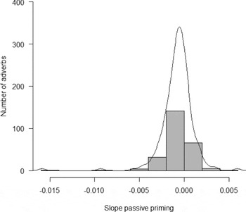
Figure 7 gives a histogram for the regression slopes for passive priming over time for all 250 adverbs, allowing closer inspection of our dependent variable.

Figure 7.

Histogram for slope coefficients for passive priming

The histogram tells us that over time there is a slight overall drift in the direction of a lower priming effect. The mean of the slopes is negative (–0.0008). While the figures are only for the 250 most frequent ly-adverb types, these account for 90 per cent of all ly-adverb tokens. So this might indicate that ly-suffixation as such is slowly becoming less analysable over time. This can be interpreted as being in line with grammaticalization theory, which would predict that the ly-affix will undergo gradual semantic, formal and syntactic attrition (Lehmann Reference Lehmann1985). That said, some individual slopes are positive, meaning that some adverbs, like practically discussed above, go against the overall drift and become more analysable over time.

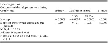
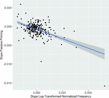
For the model design, we again ran a bidirectional variable selection procedure based on the AIC values. This procedure led us to retain only the slope coefficient for log-transformed normalized frequency as a predictor. Table 3 and figure 8 give the numeric output and the visualization of the regression model, respectively. As expected, if frequency increases over time, priming effects weaken. The slope coefficients for adverb/base ratio were excluded from the model.Footnote ⁵ The fact that changes in adverb/base ratio are no good at predicting changes in priming effects may be due to the operationalization of this predictor. As a synchronic parameter, adverb/base ratio essentially distinguishes between two groups of adverbs: those that are more frequent than their base and those that are less frequent. In our sample of 250 adverbs, however, there are only 27 adverbs that over time move from one group to the other (i.e. with an adverb/base ratio that passes over or under 1) and most of these have relatively level slopes, with a slope coefficient close to 0. In other words, there may simply not be enough adverbs in the data set for which changes in the adverb/base ratio make strong predictions.

Table 3.

Diachronic linear regression output

Figure 8.

Scatterplot with diachronic linear regression line. Adverbs that become less frequent over time tend to have a lower passive prime effect, and vice versa

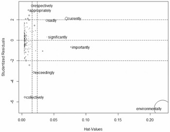
The influence plot in figure 9 reveals one potentially problematic high-leverage adverb. The adverb environmentally has a toxic combination of a low studentized residual value, a large Cook's distance and a rather extreme Hat-Value. It is the lonely dot in the lower-right corner of the scatter plot (figure 8), with a quick rise in frequency and a steeply dropping passive priming effect.

Figure 9.

Diachronic linear regression model influence plot

Because of its large Hat-Value, we refitted the regression model leaving this particular adverb out. This yields a more moderate regression slope (of –0.07), and reduces the adjusted R² value (to 0.11). The overall trend is maintained, however (with p < 0.001). The diagnostics of the latter regression model look acceptable: there is no indication of heteroscedasticity (Non-constant Variance Score Test Chi-square = 1.03, Df = 1, p = 0.311), though the residuals do not show a normal distribution (Shapiro-Wilk normality test, W = 0.95, p-value < 0.001).

In all, then, the one diachronic prediction that could be tested is borne out: changing frequency will cause changing analysability, as reflected in how sensitive a complex form is to passive priming. Again, however, it is clear that the current model can only explain a very small part of the variation that is actually observed.

7 Some comments on Martin Hilpert's response article (this volume)

In his response article to this article, Martin Hilpert investigates the replicability of our findings, by applying approximately the same procedure to a number of other derivational processes. The results are, from our point of view, somewhat disappointing: while our own case study was indeed found to be replicable in another corpus, other derivational processes, namely nominalizing -tion, nominalizing -ness, and the formation of adjectives with a negative un- prefix fail to produce the same synchronic effects. Further, our diachronic findings could not be reproduced on data from a different corpus. This warrants caution: the least one can conclude from the combined evidence in our own article and Martin Hilpert's is that any negative correlation between analysability and frequency is hard to detect in corpus data, at least when using the method we propose.

Still, there are several small and bigger differences between our case study and Martin Hilpert's replications, which we find important to point out. Hilpert's selection of case studies raises the question of comparability. Processes of word formation by -tion, -ness and un- are decidedly derivational and differ in that respect from word formation by -ly. Word formation by -tion in particular is highly irregular, with unpredictable formal transformations to the base and even forms whose base does not exist as an independent word. Further note that the use of adverbs, including ly-adverbs, is syntactically and topically less constrained than that of nouns, such as -tion and -ness derivations. Adverbs can occur in such diverse positions as left-dislocation, preverbal position and clause-final position; they are optional; and they are not so much constrained by text topic. Arguably, this greater freedom of occurrence may facilitate the manifestation of priming effects in the use of adverbs. Finally, the data from the HC that we have used may come closer to spoken usage or at least reflect less closely monitored language use than the data drawn on by Hilpert. Conceivably, priming will manifest more easily when production is less closely monitored. On each of these points, there is ample room for speculation as well as for further research.

However, we believe the most important differences between Hilpert's replications and our study are strictly methodological. The corpora Hilpert uses are smaller than the HC, and the derivational processes with -tion, -ness and un- are less frequent than adverb formation by -ly. Hilpert's results are consequently based on smaller data sets, with fewer observations per derived form. This probably means that his estimates of priming effects for each individual derived form must be somewhat less reliable. Also note that Hilpert's samples include more types (322 instead of the 250 in our analysis). It follows that they contain a larger share of low-frequency types for which it is harder to establish reliable priming measures. All of this is likely to have introduced more noise in Hilpert's data and could potentially account for a worse fit in the resultant regression models.

Specifically with respect to the diachronic replication, there are some further important differences. The time span selected for study is much longer in the replication (150 years) than in the original study (55 years). As diachronic change is operationalized by means of the coefficient of a linear regression slope, we can expect that the fit between the operationalization and the actual changes is considerably worse in the replication. This holds both for the independent variable (frequency change) and for the dependent variable (changing priming sensitivity). Hilpert's data must therefore again be noisier than ours. Further, Hilpert's analysis is based on normalized frequencies, not on log-transformed normalized frequencies. We have chosen to log-transform because otherwise frequency slopes tend to be much steeper for more frequent items. This makes intuitive sense as it is more exceptional (and we assume, linguistically more significant) for a word with 200 occurrences per million words to increase to 300 than it is for a word with 2,000 occurrences per million words to increase to 2,100. Yet frequency change for both words would have the same slope if the slope is calculated on non-transformed frequencies. Log-transformation approximately corrects for this. This is probably what explains the striking difference between Hilpert's figure 2 and our figure 8.

The upshot of all this is that Hilpert's failure to replicate our findings is not necessarily due to the absence of a negative correlation between frequency and analysability. At the same time, we have to acknowledge that Hilpert's work reveals some of the limitations of our method. In brief, the method we have tried out here will probably work well only with very large amounts of data. This brings us back to our general conclusion that the frequency effect we set out to find proves hard to detect, either because our corpus data and method are less than ideal, or because the signal is relatively weak to begin with.