


The estimation of spatial models of roll call voting has been one of the most important developments in the study of Congress and other legislative and judicial institutions. The seminal contributions of Poole and Rosenthal (Reference Poole and Rosenthal1991, Reference Poole and Rosenthal1997) launched a massive literature, marked by sustained methodological innovation and new applications. Alternative estimators of ideal points have been developed by Heckman and Snyder (Reference Heckman and Snyder1997), Londregan (Reference Londregan2000a), Martin and Quinn (Reference Martin and Quinn2002), Clinton, Jackman, and Rivers (Reference Clinton, Jackman and Rivers2004), and Poole (Reference Poole2000). The scope of application has expanded greatly from the original work on the U.S. Congress. Spatial mappings and ideal points have now been estimated for the Supreme Court (Bailey and Chang Reference Bailey and Chang2001); Bailey, Kamoie, and Maltzman (Reference Bailey, Kamoie and Maltzman2005); Martin and Quinn (Reference Martin and Quinn2002), U.S. presidents (McCarty and Poole Reference McCarty and Poole1995), a large number of non-U.S. legislatures (Londregan Reference Londregan2000b; Morgenstern Reference Morgenstern2004), the European Parliament (Hix, Noury, Roland Reference Hix, Noury and Roland2006; Reference Hix, Noury and Roland2007), and the U.N. General Assembly (Voeten Reference Voeten2000).
The popularity of ideal point estimation results in large part from its very close link with theoretical work on legislative politics and collective decision making. Many of the models and paradigms of contemporary legislative decision making are based on spatial representations of preferences. Consequently, estimates of ideal points are a key ingredient for much of the empirical work on legislatures, and increasingly on courts and executives.Footnote 1 This has contributed to a much tighter link between theory and empirics in these subfields of political science.
Unfortunately, the literature on state politics has generally not benefited nearly as much from these developments. To be sure, there is a small and growing set of studies that have estimated ideal points of state legislators using roll call data (Aldrich and Battista Reference Aldrich and Battista2002; Bertelli and Richardson Reference Bertelli and Richardson2004, Reference Bertelli and Richardson2008; Gerber and Lewis Reference Gerber and Lewis2004; Jenkins Reference Jenkins2006; Kousser, Lewis, and Masket Reference Kousser, Lewis and Masket2007; McCarty, Poole, and Rosenthal Reference McCarty, Poole and Rosenthal2006; Wright Reference Wright2007; Wright and Clark Reference Wright and Clark2005; Wright and Winburn Reference Wright and Winburn2003). But empirical applications of spatial theory to state politics have been limited by two important factors. The first is that roll call voting data over time have not been collected for all 50 states. The efforts of Gerald Wright (Wright Reference Wright2007) have resulted in a set of roll call data across all 50 states, but only for a single two-year period. Longer time series exist only for a handful of states (e.g., Lewis Reference Lewis2010).
The second impediment is that because ideal points are latent quantities, direct comparisons across states or even between chambers within the same state are generally difficult to make. The researcher can only directly compare two legislators from different chambers if they vote on identical legislation in both. Some scholars attempt to avoid this problem by assuming that legislators maintain consistent positions over time and as they move from one legislature to another. To the extent that such assumptions are reasonably valid, approximate temporal and cross-sectional comparisons can be made. But this approach has only limited utility in state politics. A recent article (Shor, Berry, and McCarty Reference Shor, Berry and McCarty2010) exploited the voting records of legislators who graduated from a state legislature to Congress to produce a common spatial map for state and congressional politics. Using the assumption that legislators are ideologically consistent on average, they were able to rescale within-state legislative scores into a congressional common space. Unfortunately, this approach works only for the small handful of states where there is sufficient mobility between the state legislature and the U.S. Congress.
The conjunction of these two problems reduces the scope of spatial theory in state politics to a choice between examining within-state variation for a handful of states or making dubious comparisons on a cross section of states. Truly comparative work using the spatial model has been elusive, and attempts to overcome these limitations have been unsatisfactory. One approach is to use interest group ratings in lieu of ideal points. But the problems with using interest group ratings as measures of ideal points are well known (McCarty Reference McCarty, Schickler and Lee2011; Snyder Reference Snyder1992). In particular, interest group ratings suffer from exactly the same comparability problems as ideal point estimates (Groseclose, Levitt, and Snyder Reference Groseclose, Levitt and Snyder1999). As we discuss later, the issues of comparison across states are considerably more daunting than those of temporal comparison.
Berry et al. (Reference Berry, Ringquist, Fording and Hanson1998) take a different approach. To produce annual estimates of government ideology for all 50 states over time, they combine measures of the ideology of each state's congressional delegation with reweighted data on state legislative seat share. These aggregate measures have been heavily utilized in the literature on state politics and policy. These measures, however, suffer from two potential problems. First, because the measures are aggregates, they reveal little about heterogeneity, especially intraparty heterogenerty, within states. Indeed, there are no individual-level measures of legislator ideology. Second, the validity of the Berry measure depends on the heretofore untested assumption that the ideological position of a state party's delegation to Congress is a good proxy for that of its delegation in the state legislature. We will present evidence that undermines this assumption.
In this article, we tackle both these potential problems with state-level applications of the spatial model. First, we introduce a new data set of state legislative roll call votes that covers all state legislative bodies over approximately a decade. These data currently cover the period from 1993 to 2009, but with variation in coverage across the states. Second, we employ a new strategy to establish comparability of estimates across chambers, across states, and across time. Here we use a survey of legislative candidates at the state and federal levels over a number of years. Importantly, the survey questions are asked in an identical form across states, and many questions are repeated over time. Thus, the survey allows us to make cross-state, cross-chamber, and over-time comparisons. The survey, however, does not provide any information about nonrespondents. But as we justify later in text, we can use the combination of the survey and roll call voting data to estimate ideal points for all state legislators serving during our coverage period that are comparable across states and with the U.S. Congress.
These new estimates open new avenues for inquiry, not just in state politics, but in legislative politics more generally. In particular, our spatial mapping not only adds a much needed cross-sectional element to empirical work on legislative institutions, but also will allow scholars to exploit institutional variation in ways not previously possible. Thus, our measures may be central in adjudicating claims about the effects of districting reform, open primaries, term limits, recall, and voter initiatives. Our data may also be useful to those wishing to understand the political origins of the state fiscal crises of the last decade. Although it is not possible to do full justice to any of the new potential applications here, we discuss and illustrate several.
The article proceeds as follows. First, we discuss the methodological issues associated with comparing ideal point estimates across different legislatures and over time. Specifically, we demonstrate how the survey of candidates can be used to ameliorate these problems. Then, we describe both our survey-based data and our procedures for collecting roll call voting data from the states. We also discuss the results obtained using surveys and roll calls separately. Subsequently, we link the survey and roll call estimates to generate a common scaling of the state legislatures and Congress. We focus on validating the model in terms of fit and dimensionality as well as on comparing the estimates with other individual and aggregate measures of ideology. Finally, we sketch several substantive applications related to representation, polarization, and parties and then conclude.
THE COMPARABILITY OF IDEAL POINTS
To grossly simplify, statistical identification of ideal points comes from data on how often legislators vote with other legislators on a common set of roll calls. We identify legislators as conservatives because they are observed voting with other conservatives more frequently than they are observed voting with moderates, which they do more often than they vote with liberals. But when two legislators serve in different bodies, we cannot make such comparisons. Being a conservative in the Alabama House is quite different from being a conservative in the Massachusetts Senate.
The concern about comparability of ideal point estimates is a long standing one. There have been efforts to produce common ideological scales for the U.S. House and Senate (Groseclose, Levitt, and Snyder Reference Groseclose, Levitt and Snyder1999; Poole Reference Poole1998), for presidents and Congress (McCarty and Poole Reference McCarty and Poole1995), for presidents, senators, and Supreme Court justices (Bailey and Chang Reference Bailey and Chang2001; Bailey, Kamoie, and Maltzman Reference Bailey, Kamoie and Maltzman2005), and for Supreme Court and Court of Appeals justices (Epstein et al. Reference Epstein, Martin, Segal and Westerland2007). Similar issues arise in the estimation of dynamic models (Martin and Quinn Reference Martin and Quinn2002; Poole and Rosenthal Reference Poole and Rosenthal1997).
Identification of the models relies on the existence of bridge actors who cast votes (or make votelike decisions) in multiple settings. For example, Bailey and Chang (Reference Bailey and Chang2001) compare Congress and the Supreme Court by relying on the fact that legislators often opine on the cases that the justices have voted on. In most cases, however, the bridge actors are not making decisions in different venues contemporaneously; typically, they serve in different legislatures sequentially. Common scales are identified by assumptions about the consistency of behavior when a bridge actor moves from one setting to another. For example, Shor, Berry, and McCarty (Reference Shor and Rogowski2010) rely on bridge actors who first served in a state legislature and later on in Congress. The key assumption is that, on average, bridge actors' ideal points do not change as they move to Congress.Footnote 2 Unfortunately, the paucity of legislators in many states who moved to Congress in the past decade makes producing comparable estimates difficult for all but a few states.
Given the limitations of using bridge legislators to link states, we use the Project Vote Smart National Political Awareness Test (NPAT), a survey of state and federal legislative candidates. We use this survey, which we describe in more detail in the next section, to estimate the ideal points for all the respondents. But because the response rate of the survey is far from 100%, the survey provides ideal points for only a fraction of state legislators. So we supplement the NPAT data with roll call voting data from all 50 states in the past 15 years. Under the assumption that the legislator uses the same ideal point when answering surveys as he or she does when she votes on roll calls, the NPAT survey bridges ideal point estimates from one state to another.Footnote 3
Our procedure is as follows. We use both of Poole (Reference Poole2005)'s methods to estimate a common spatial map using bridges. We pool congressional members' and state legislators' responses to the NPAT questionnaire. Using answers to the common questions as the bridges, we scale all of these respondents to derive a common NPAT space score for each legislator in one and two dimensions. This produces directly comparable scores for responding members of Congress and state legislators.
Next, we estimate comparable ideal point estimates for the NPAT nonrespondents in Congress and state legislatures. We accomplish this by scaling Congress and each state legislature separately using a roll call database that covers all legislators. Thus, we have two scores—a roll call–based score that covers all legislators but is not comparable across states and an NPAT score that covers fewer legislators but is in a common space.
We translate the roll call–based state legislative scores to NPAT common space via a least-squares regression on each dimension. Using the regression parameters, NPAT common space scores are imputed for the nonrespondents. Because all predicted scores are now on the same scale, they can be directly compared across states (and Congress itself). It is important to remember that the NPAT common space scores are rescaled roll call ideal points for both nonrespondents and respondents.
In this article, we use Bayesian item-response theory models to estimate the spatial models (Clinton, Jackman, and Rivers Reference Clinton and Meirowitz2004; Jackman Reference Jackman2000, Reference Jackman2004; Martin and Quinn Reference Martin and Quinn2002).Footnote 4 We performed the same analysis with Poole–Rosenthal NOMINATE scores (Poole and Rosenthal Reference Poole and Rosenthal1991). The estimates of ideal points correlate extremely strongly across methods, which is to be expected given what we know about the performance of these two procedures in data-rich environments (Carroll et al. Reference Carroll, Lewis, Lo, Poole and Rosenthal2009; Clinton and Jackman Reference Clinton and Jackman2009).
DATA
NPAT Survey
The NPAT is administered by Project Vote Smart, a nonpartisan organization that disseminates information on legislative candidates to the public at large.Footnote 5 The data used in this article are based on the surveys they conducted from 1996 to 2009.
The questions asked by Project Vote Smart cover a wide range of policy issues, including foreign policy, national security, international affairs, social issues, fiscal policy, environmentalism, criminal justice, and many more. Most of the survey questions are asked in a yes or no format so that the data have a form very similar to that of roll call voting.
Despite the richness of these data, use of the NPAT surveys has been limited. Ansolabehere, Snyder, and Stewart (Reference Ansolabehere, Snyder and Stewart2001b) use the 1996 and 1998 surveys to distinguish between the influence of party and preferences on roll call voting (see also Snyder and Groseclose Reference Snyder and Groseclose2001 in response to McCarty, Poole, and Rosenthal Reference McCarty, Poole and Rosenthal2001), whereas Ansolabehere, Snyder, and Stewart (Reference Ansolabehere, Snyder and Stewart2001a) use the survey to study candidate positioning in U.S. House elections. One problem with the NPAT survey is that response rates are declining over time. A majority of state legislative incumbents answered the survey in the 1990s, but currently only about one-third do in each state. Our approach, however, avoids the effects of nonresponse bias. As long as legislators are ideologically consistent (on average) across surveys and roll calls, our imputed NPAT ideal points have almost universal coverage.
The questions on the NPAT do change somewhat over time. But although hot political topics such as stem cell funding come and go, many questions such as those pertaining to abortion and taxes are consistently asked. Most useful for our purposes, the vast majority of the questions asked of state legislators are identical across states. This large set of common questions provides significant support for making cross-state comparisons. Moreover, the NPAT asks dozens of questions that are common to the states and the U.S. Congress. This allows us to link our state legislative ideal points to those of U.S. senators and representatives. Because we bridge legislatures over time by estimating a single ideal point for each legislator, we do not allow for ideological drift by individuals except when they switch parties.Footnote 6 In total, we have 5,747 unique questions, over the years 1996–2009, for incumbents in the state legislatures and Congress. This produces a sample of 563 members of Congress and 5,638 state legislators.
Although politicians may have incentives not to answer the NPAT, the response rates are impressive. As we have noted, however, response has declined over time. There is also substantial variation in these rates across states. Iowa and Virginia have the lowest response rates, with 19% of their legislators answering the survey, whereas Nebraska has the highest, at 52%. The overall rate is about one-third. We address possible implications of nonresponse bias later in text, both for the use of NPAT-based preference measures and for our bridging procedure.
Roll Call Data
Our state roll call data are from a project supported by the Woodrow Wilson School and the Russell Sage Foundation.Footnote 7 Journals of all 50 states (generally from the early to mid-1990s onward) have been either downloaded or purchased. Hard copies of journals were disassembled, photocopied, and scanned. These scans were converted to text using optical character recognition (OCR) software. To convert the raw legislative text to roll call voting data, we coded many data-mining scripts in Perl. Because the format of each journal is unique, a script was developed for each state and each time a state changed its presentation format. The use of OCR does genenerate mistakes, but the recognition rate is around 98%. Our roll call dataset now covers all 50 states and more than 18,000 state legislators.
Scaling Individual State Legislatures
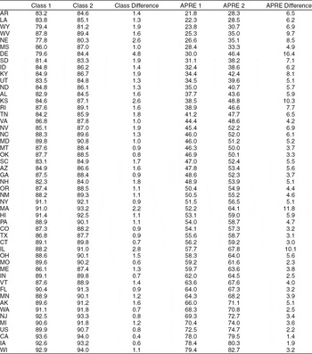
For each state, we estimate one- and two-dimensional spatial models using the Bayesian item response model.Footnote 8 We begin with an examination of the predictive power of the spatial model for explaining patterns of roll call voting within each state. Following Poole and Rosenthal (Reference Poole and Rosenthal1991, Reference Poole and Rosenthal1997), we assess the models based on the overall classification success as well as the aggregate proportionate reduction in error (APRE).Footnote 9 Table 1 provides these measures for all states for a one-dimensional model as well as the improvement from adding a second dimension.
Fit Statistics for Pooled State Legislatures and Congress
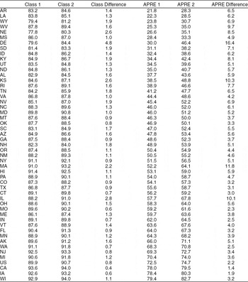
Note: Reported are classification and aggregate proportionate reduction in error (APRE) in one and two dimensions. Table is sorted by APRE in one dimension.
Not surprisingly, there is considerable variation in the classification success of the spatial model. The one-dimensional model ranges from 78% for Nebraska to 94% for California, and APRE ranges from 22% for Arkansas and Louisiana to 79% for Wisconsin. In comparison, a one-dimensional spatial model correctly classifies 90% for the 103rd–11th Congresses (1993–2009) while reducing the error rate of the null model by 73%. Table 1 also shows that the improvements associated with a two-dimensional model are modest, but larger than that for Congress. Average classification increases only 1.4% (compared with less than 1% for Congress), and average improvement in the APRE is larger (5.5%) than that for Congress (2.1%). On the other hand, California and Wisconsin, two of the most polarized states, have unambiguously better fit statistics than does Congress. Of course, there are individual states for which the second dimension is important. Four states—ranging from very liberal to very conservative—have APRE improvements of 10% or more (Delaware, Illinois, Kansas, and Massachusetts).
Despite significant cross-state variation, it appears that, similarly to Congress (Poole and Rosenthal Reference Poole and Rosenthal1991, Reference Poole and Rosenthal1997) and many other institutions (Poole and Rosenthal Reference Poole and Rosenthal2001), a single dimension explains the vast bulk of the voting in state legislatures. On one hand, this is somewhat surprising. One might expect that differences in institutional rules, party systems, and issue agendas would manifest themselves in more important higher dimensions. Alternatively, such a finding is consistent with the idea that in the current era of heightened left–right polarization, political conflicts in the states may have become more reflective of the national political conflict. Unfortunately, we do not have the data to examine whether the dimensionality of state politics were higher in earlier periods when politics were more localized and less polarized.
THE NPAT COMMON SPACE
If computational costs were not a consideration, we could estimate common-space ideal points directly using item-response models or NOMINATE. This procedure would involve stacking a very large roll call matrix of all state legislative votes for every state and every year on top of the matrix of NPAT responses and estimating the desired model. But the cost of such an approach is significant.
Instead we take a two-step approach. After estimating roll call–based ideal points for all legislators in each state, we project them into the space of NPAT ideal points using ordinary least squares (OLS). The fitted values of these regressions generate predicted NPAT scores for the nonrespondents.Footnote 10 Note that each state has its own specific mapping parameters. This allows us to map ideology from the idiosyncratic roll call space of each state into the NPAT common space.
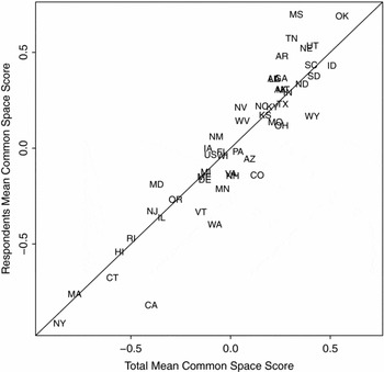
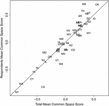
To validate our measures, we must address a number of concerns. First, a key question in using NPAT surveys in cross-state research is whether their samples are ideologically representative of the universe of state legislators. This is less a concern for our method, because our Monte Carlo work suggests that the sample of bridge actors or issues need not be representative, just as OLS does not require the independent variables to be drawn representatively (Shor, McCarty, and Berry Reference Shor, McCarty and Berry2008). Our procedure, however, allows us to assess how ideologically representative NPAT respondents are. Using our bridged estimates for what is close to the universe of state legislators, Figure 1 plots the average score for responders and the state as a whole. A one-sample t-test reveals that, at the p < .05 level, respondents in 10 states are significantly different from the full population.Footnote 11 In seven states, Republican respondents differ from the population of Republican legislators, whereas this is true of Democrats in four states.Footnote 12 Despite these differences, overall the NPAT responses appear to be fairly representative. To the extent that they are not, we count this as an argument for using our method rather than ignoring nonresponse bias and using NPAT scores by themselves.
Representativeness of NPAT Responders
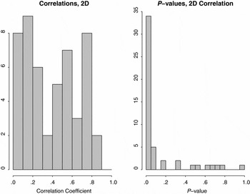
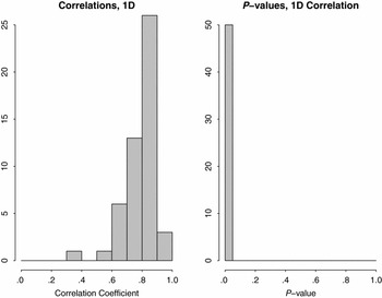
A second concern is that our method requires that the NPAT survey tap into the same issue dimensions that divide legislators on roll call voting. If the primary ideological dimension varies across states and is different from that obtained by scaling the NPAT, the survey could not successfully bridge legislators from different states. Heightening this concern is that the NPAT asks about a much broader array of economic, social, and foreign policy issues than are found on the typical state legislative agenda. We find, however, that ideal point estimates obtained for state legislators using the NPAT correlate very well with those obtained from state roll call votes. Figure 2 provides a histogram of the correlations of the NPAT ideal points with the roll call ideal points. Although there is variation (mostly attributable to the variation in the number of NPAT respondents by state), the correlations are generally quite high and always statistically significant.
Correlation of First Dimension NPAT Scores with First Dimension State Roll Call Scores

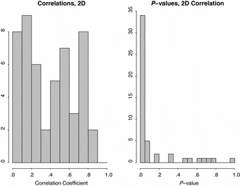
Although we focus primarily on bridging the first dimension, it is interesting that the NPAT second dimension tracks the roll calls' second dimension for a very large number of states. Figure 3 shows the histogram of correlations on the second dimension. The correlations are not as high as for the first dimension but are statistically significant for the vast majority of states. So although there is some cross-state variation in the content of the second dimension, the NPAT scores generally do a good job of capturing it.
Correlation of Second Dimension NPAT Scores with Second Dimension State Roll Call Scores
A third concern is the extent to which positions on roll call measures deviate from NPAT measures on the basis of partisan or electoral pressures. Ansolabehere, Snyder, and Stewart (Reference Ansolabehere, Snyder and Stewart2001b) point out that ideal points of U.S. House members estimated by roll call voting tend to be more polarized across parties than ideal points estimated using the NPAT. They attribute this difference to the effect of partisan pressure, which influences roll call voting but is not present in the survey response.
To understand how we can account for party effects, consider the following error-in-variables specification. Let x i be the ideal point of legislator i estimated from roll call voting and x i* the true ideal point. We can now capture party differences in the link between true ideal points and those estimated from roll call votes as follows. Let


where γR and γD are party effects and ϵi are other sources of measurement error, assumed to have mean zero.Footnote 13 Ansolabehere, Snyder, and Stewart (Reference Ansolabehere, Snyder and Stewart2001b) assume that roll call records are more conservative than the true ideal points for Republicans and more liberal for Democrats. Given the convention of assigning higher scores for conservative positions, this implies that γR > 0 and γD < 0. Because the scale of ideal points is only identified up to a linear transformation, we cannot identify each party effect separately. So we instead estimate γ =γR − γD/2, which Ansolabehere, Snyder, and Stewart (Reference Ansolabehere, Snyder and Stewart2001b) predict to be positive. Consequently we assume that the relationship between the true ideal point x i* and the observed roll call ideal point is given by

where R i = 1 if legislator i is a Republican, 0 if he or she is an independent, and −1 if he or she is a Democrat.
Now let n i be the estimated ideal point from the NPAT survey. Suppose we tried to estimate the projection of x i*,

If we used only x i, we would have

Note that the error term of the projection contains βγR i, which is clearly correlated with x i*. Therefore, estimates of α and β will be biased if γ ≠ 0. In that case, we would have to include R i in the projection of x i to n i to obtain the correct relationship between x i* and n i. To test for this possibility, we estimate for each state j

where θj = −βj γj. It is the fitted values from this regression that we use to estimate n i for those legislators who do not respond to the NPAT. This procedure would also correct for the possibility that NPAT scores were more moderate than roll call scores. In that case, however, γj < 0, so θj > 0.
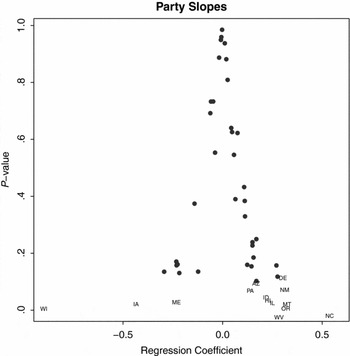
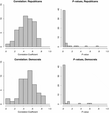
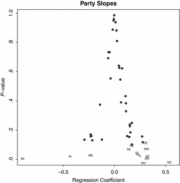
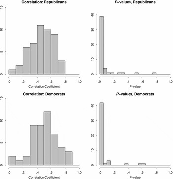
Despite these concerns, however, partisan biases between observed NPAT and roll call ideal points do not appear to be especially important. Figure 4 plots the distribution of estimates of θj. Note that most of these estimates cluster around zero and have high p-values. Moreover, within-party correlations are large and highly significant, if less so than the pooled correlations because of reduced sample size (especially for states dominated by a particular party). Figure 5 shows that this is true for both Republicans and Democrats. Given these mixed results on party effects, we will focus on the results of our party-free (i.e., θj = 0) NPAT common scores. Those with a partisan adjustment will be made available when the data are released publicly.
Party Slopes and P-values
Within-party Correlations of NPAT and State Roll Call Scores for Republicans and Democrats
Comparing States
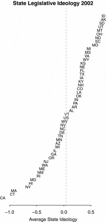
Having addressed several potential concerns about our method, we turn to a description of our NPAT common space estimates. The distributions of the common space NPAT scores aggregated at the state level are illustrated for a single year, 2002, in Figure 6. We include the U.S. Congress for purposes of comparison. California, Connecticut, and Massachussetts anchor the liberal end of the spectrum, whereas Idaho, Alaska, and South Dakota do the same for the conservative end.
Plot of Averaged State Chamber Medians for 2002
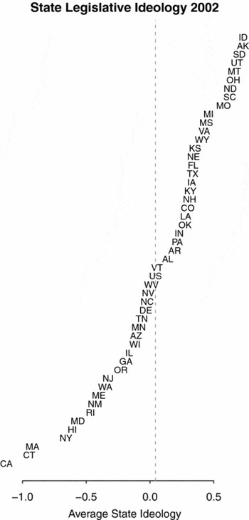
Figure 7 shows the distributions of scores by party, pooled across time within states. One of our most striking findings is the tremendous variation in polarization across states. This manifests itself in the variance of party medians and the extent of overlap of party distributions within states. There is also a large amount of overlap among the party medians across states. For example, the Democratic party in Mississippi is more conservative than the relatively liberal Republican parties of Connecticut, Delaware, Hawaii, Illinois, Massachusetts, New Jersey, New York, and Rhode Island. The liberal Republicans of New York locate to the left of relatively conservative Democratic parties in Alabama, Arkansas, Kentucky, Louisiana, Mississippi, North Dakota, Oklahoma, South Carolina, South Dakota, and West Virginia. Despite the historical decentralization of the American party system, it is surprising that this much overlap remains.
Box Plot of Estimated NPAT Common Space Scores for Pooled State Legislatures Compared with Scores for Congress (with Vertical Lines Drawn at the Pooled Congressional Party Medians)

It has been argued that the Democratic and Republican parties differ significantly in terms of their levels of discipline and cohesiveness (e.g., Hacker and Pierson Reference Hacker and Pierson2005). Although this may be true of representatives in Congress, our data suggest that the median positions of the two parties vary equally across states. The standard deviations of the pooled state party medians are 0.38 and 0.33 for Democrats and Republicans, respectively. We cannot reject the null hypothesis of no difference.
State Legislative and Congressional Delegations
One of the primary advantages of our measures is that we can compare the ideological compositions of state legislatures with those of state delegations to Congress. This not only allows us to consider questions about differences in representation at the state and national levels, but also allows us to consider the major assumption of state-level ideology scores based on congressional ideal points (Berry et al., Reference Berry, Ringquist, Fording and Hanson1998; Reference Berry, Fording, Ringquist, Hanson and Klarner2010).
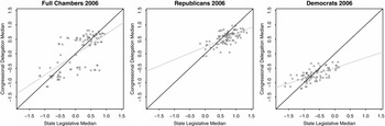
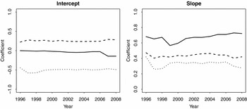
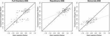
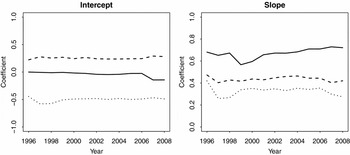
As an illustrative example, we consider 2006. On the left side of Figure 8, we plot the state legislative chamber and party medians against the median of each state's full and partisan congressional delegations. Regressing the congressional delegation median on the state legislative median, we find that the intercept is approximately zero for the full chamber, positive for Republicans, and negative for Democrats. The slopes are always less than one for each comparison. Congressional delegations appear to inhabit an ideological space that is more restricted than that of state legislative chambers, and there is a considerable disconnect between the two at the left and right ends of the space. Figure 9 extends the comparison for 1996–2008 through a series of cross-sectional regressions for each year. On the whole, 2006 appears fairly representative.
Scatterplot of State Legislative Chamber, Republican, and Democratic Medians (x-axis) against Full State, Republican, and Democratic Congressional Delegation Medians (y-axis)
Coefficients from Repeated Cross-sectional Regressions of Congressional Delegations on Chamber and Party Medians
Interest Group Ratings
Interest group ratings have been used as a roll call–based measure of legislator ideology in the literature. One advantage of such scores is that more than one organization produces ratings for most state legislatures. Here we look at ratings from two conservative groups—the National Federation of Independent Business (NFIB) and the National Rifle Association (NRA)—and two liberal organizations—the AFL-CIO and the League of Conservation Voters (LCV).
For example, Overby, Kazee, and Prince (Reference Overby, Kazee and Prince2004) use NFIB ratings to examine committee representativeness in 45 states. Ranked by Fortune magazine as the most influential business lobby, the NFIB has 350,000 members and affiliates in all 50 state capitols plus Washington, DC. The conservative organization takes public positions on a small number of bills that receive roll call votes that relate to business in the state legislatures, such as tort reform. Legislators who vote in perfect alignment with the state NFIB position receive a score of 100, and those who vote not at all with the NFIB receive 0. In 2007–2008, for example, the NFIB considered five House and six Senate votes in the Illinois ratings, including those on tax increases, a resolution on the Employee Free Choice Act (“card check”), the governor's universal health care plan, and an expansion of the Family and Medical Leave Act.
A few issues appear to make the use of interest group ratings for comparative research problematic. The first is the lack of a common agenda across states. When state chapters of national organizations score floor votes, we doubt they are using a comparable scale across states. Second, because agendas change over time even within states, scores will not be comparable over time (Groseclose, Levitt, and Snyder Reference Groseclose, Levitt and Snyder1999). Third, without sufficient bridging observations, scores are not even comparable across chambers within states. Finally, even were all this not the case, using a small handful of bills to score legislators inevitably leads to a loss of much information in capturing the underlying ideology of legislators.
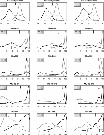
We collected 10,271 NFIB ratings (49 states), 7750 NRA ratings (41 states), 5819 AFL-CIO ratings (20 states), and 6,915 LCV ratings (29 states) for 2004, 2006, and 2008. When aggregated, the scores produce a rather peculiar distribution. Figure 10 shows that the mean Republican scores are extremely right-skewed for the conservative interest groups, and equally left-skewed for one of the two liberal ones (AFL-CIO). For these three groups, members of the favored party are barely differentiated from each other, whereas the opposing party does not converge on any dominant position. The LCV scores show less skew, but they also show far more overlap for legislators (and are available for only a subset of states).
Density Plots of Special Interest Group Ratings for State Legislators, 2004–08 (Dark Lines Are Democrats and Light Lines Are Republicans)

Interest group scores are correlated positively in the cross section with common space scores. This correlation masks considerable heterogeneity and some unexpected outcomes. For example, small but significant numbers of chambers either had no variation at all in interest group scores, or the interest group scores were not significantly related to common space scores, and worst of all, some interest group scores were negatively related to common space scores.Footnote 14
Aggregated Scores
To what degree are the congressional common space scores for the state legislatures in this article consistent with other measures of state ideology? We start the comparison with Berry et al. (Reference Berry, Ringquist, Fording and Hanson1998)'s popular state elite ideology scores. They are derived from a formula that is a weighted average of party proportions in both chambers multiplied by state delegation congressional ideology.Footnote 15
We replicate the Berry scores, but with some slight modifications. We do so for two reasons. First, we strip out the inferred gubernatorial ideology, because we do not have common space scores for governors to compare. However, because the governor's position is itself merely the average of own-party ideology, it is only a reweighting of the inferred legislative ideology. We also separate the component calculations for the upper and lower chambers to have a more fine-grained comparison between the two series of scores. We thus generate what we call Berry component scores for two chambers in 49 states (excepting Nebraska) over 1995–2007.Footnote 16
As we have shown, measures of congressional delegations are quite imperfect as proxies for those of state legislatures. But what effect does this have on the Berry component scores? We investigate this question longitudinally and cross-sectionally. That is, within each state (or year), to what degree are the Berry component scores correlated with congressional common space chamber medians?
There are some significant differences between the Berry component scores and ours. The annual cross-sectional correlation coefficients average 0.77 and 0.85 for the upper and lower chamber. But the cross-sectional correlations of party proportions to scores are almost as high, averaging around 0.65 and 0.72.
The longitudinal relationship between the Berry component and NPAT scores, on the other hand, is considerably weaker.Footnote 17 Longitudinal correlations between the Berry component scores and common space chamber medians were insignificant (p > .10) in 29 of the 98 chambers, and significant and incorrectly signed in 6 of them. Both chambers in Massachusetts were assessed to be more liberal over time, whereas in fact they became more conservative. Party proportions correlate slightly better, with only 20 insignificant and 3 wrongly signed correlations.Footnote 18
Although the low correlations between the Berry and NPAT scores may result from limitations of either methodology, we believe that the weaker-than-expected connection between congressional and state legislative party delegations results in Berry measures that are inadequate to capture trends in state ideology over time.
APPLICATIONS
Representation in State Legislatures
Our data allows us to consider the extent to which state legislators are representative of the ideology of their district. For districts in the U.S. House, the typical approach is to employ some proxy, such as U.S. presidential vote, perhaps supplemented with other data (Levendusky, Pope, and Jackman Reference Levendusky, Pope and Jackman2008). Unfortunately, presidential vote data are generally unavailable at the state legislative district level.
As a second best alternative, we obtained county-level presidential vote data from Leip (Reference Leip2008), and then we imputed the presidential vote for legislative districts. The principal difficulties in using this imputation approach are places where multiple districts are embedded within a county,Footnote 19 or places where counties cross district lines or vice versa. In addition, districts from states that assign nonstandard names (Alaska, Massachusetts, Vermont) could not easily be merged and were dropped. We validated the imputed vote for districts by comparing the imputed vote in the upper and lower chambers against the actual presidential vote for 2004 for Texas, a state for which data at the state legislative district level are available, in those chambers. The correlation coefficients were greater than 0.8 for both district types, and quite statistically significant. Though noisy, the imputation is reasonably accurate.
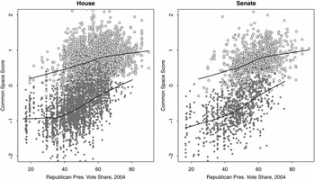
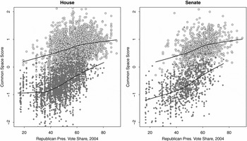
To begin with, we compare the imputed 2004 presidential vote with legislator ideology from 2005 (e.g., following the 2004 November election). The two are highly correlated, both within and between parties, as can be seen in Figure 11. The picture is quite similar to that of the relationship between the ideologies of members of Congress and their constituencies; a cloud of Republicans in the upper right, a cloud of Democrats in the lower left, and a substantial gap between the two at any fixed level of presidential support.
Scatterplot of Imputed 2004 Presidential Vote by Legislative District (X-axis) for Upper and Lower Chambers, against 2005 Common Space Ideal Points
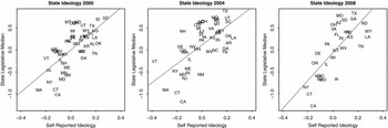
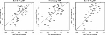
We also can assess representation at the state level. Here we consider how cross-state variation in voter preferences accounts for variation in the overall and party medians of state legislatures. For measures of voter preferences, we aggregate the self-reported ideology questions from the 2000–08 Annenberg National Election Surveys. Of course, because these measures are on different scales, we can only address responsiveness, not congruence.Footnote 20 Figure 12 plots the mean voter ideology self-placement against the pooled legislative median for each state. Although the lack of common scale prevents us from evaluating congruence, the strong correlations indicate a substantial amount of responsiveness between voter preferences and legislative medians.
Scatterplot of Averaged (Upper and Lower Chamber) Legislative Medians (x-axis) in 2000, 2004, and 2008 against Annenberg Survey State Mean Standardized Self-reported Ideology (y-axis)
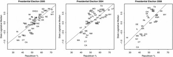
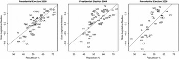
An alternative approach compares presidential vote shares to legislative medians. Figure 13 shows that the correlation between the two is quite strong for the 2000, 2004, and 2008 elections, supporting the notion that state legislators are ideologically responsive to their electorates.
Scatterplot of Averaged (Upper and Lower Chamber) State Legislative Medians (x-axis) in 2000, 2004, and 2008 against Presidential Election Results Expressed as the Republican Two-party Vote Share (y-axis)
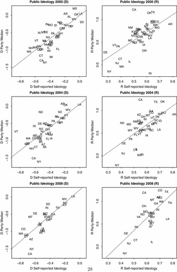
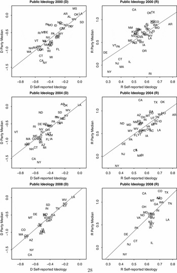
Our measure also allows us to disaggregate legislative ideology by party to assess the extent to which state party medians are responsive to the preferences of their voting constituencies. Figure 14 plots mean ideological placement by party against the legislative party medians. Again, the level of responsiveness is quite impressive.
Scatterplot of Averaged (Upper and Lower Chamber) Legislative Party Medians (x-axis) in 2000, 2004, and 2008 against Annenberg Survey State Mean Standardized Self-reported Ideology (y-axis) for Self-Identified Members of Each Party
Polarization
Studies of the U.S. Congress find that parties have become highly polarized in Congress in recent years (Layman, Carsey, and Horowitz Reference Layman, Carsey and Horowitz2006; McCarty, Poole, and Rosenthal Reference McCarty, Poole and Rosenthal2006; Poole and Rosenthal Reference Poole and Rosenthal1984); Theriault (Reference Theriault2008). Due to the lack of data, scholars have not been able to ascertain whether such a trend is apparent at the state level. The new data estimated in this article can more definitively answer this question.
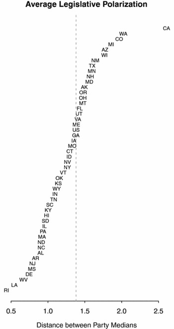
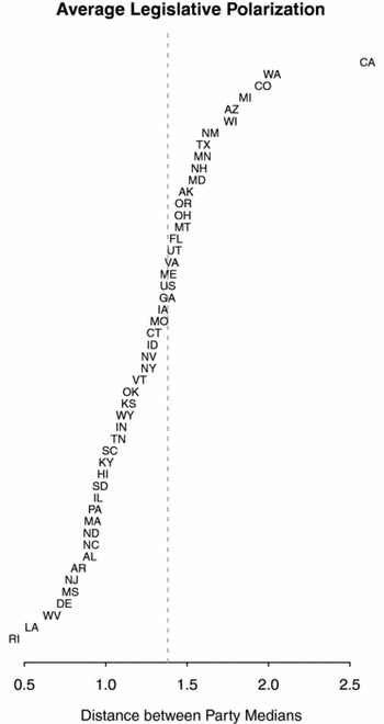
Figure 15 shows that polarization at the state legislative level is real, at least for the previous 15 years.Footnote 21 Moreover, it reveals how much polarization varies across states. In comparison to Congress, the majority of state legislatures are less polarized, whereas 15 are actually more polarized. California is by far the most polarized state legislature, and Congress looks decidedly bipartisan by comparison.Footnote 22 On the other end, Rhode Island and Louisiana are the least polarized. In the former, Democrats are liberal, but so too are Republicans. In the latter, the converse is true.
Plot of Mean Levels of State Legislative Polarization (Measured by Distance between Party Medians) over the Full Time Period Available for Each State, Averaged between Both Chambers
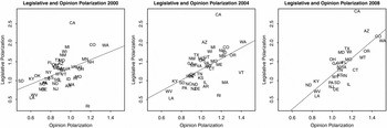
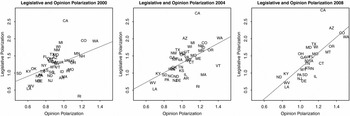
What can account for the spatial variation in polarization? One simple account links ideological polarization in the legislature to a divide in the electorate. Figure 16 illustrates that the two are indeed strongly correlated.
Scatterplot of Difference in Legislative Party Medians (x-axis) against Difference in Average Self-reported Ideology by Self-identified Partisans in the 2000, 2004, and 2008 Annenberg Surveys (y-axis)
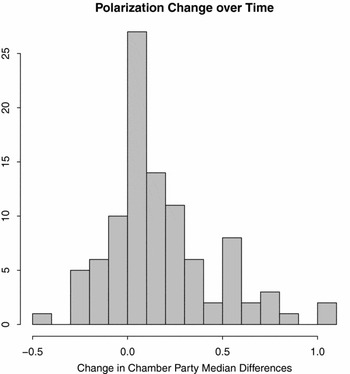
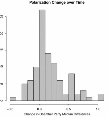
What about longitudinal variation within states? Figure 17 illustrates that polarization is an ongoing process, but does not move in a strictly upward fashion over time. Even over a comparatively short time period, most states continue to experience increased polarization, whereas a significant minority are apparently depolarizing (22 chambers in total).
Histogram of Changes in Polarization for All 98 State Legislative Chambers (Omitting Nebraska), as Measured by the Difference in Levels of Polarization from the First to the Last Year Available
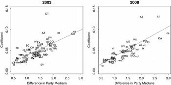
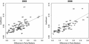
Next, we examine the possibility that legislative polarization enhances representation. Although polarization is often reviled in the popular and research literatures for coarsening politics and turning off voters, others have hailed the rise of this phenomenon as undergirding the ideological distinctiveness of American political parties. The clearer brand names that result give voters an easier decision rule at the ballot box and allow them to vote more reliably for the more ideologically proximate alternative. When parties overlap ideologically, it is less clear for whom to vote. Figure 18 shows that increased polarization within a chamber is associated with a stronger relationship between presidential voting behavior (presumably driven by more ideological concerns) and legislator ideology.
Plot of Slope Coefficients (at p < .10) from Repeated Cross-Sectional Regressions of Legislative Ideology on District Ideology, Plotted against State Legislative Chamber Polarization (Measured as the Difference in Party Medians), for 2003 and 2008
McCarty, Poole, and Rosenthal (Reference McCarty, Poole and Rosenthal2009) point out that partisan polarization can be decomposed into roughly two components. The first part, which they term intradistrict divergence, is simply the difference between how Democratic and Republican legislators would represent the same district. The remainder, which they term sorting, is the result of the propensity for Democrats to represent liberal districts and for Republicans to represent conservative ones.
To formalize the distinction between divergence and sorting, we write the difference in party mean ideal points as

where x is an ideal point, R and D are indicators for the party of the representative, and z is a vector of district characteristics. We assume that z is distributed according to the density function f and that p(z) is the probability that a district with characteristics z elects a Republican. The term p is the average probability of electing a Republican. The average difference between a Republican and Democrat representing a district with characteristics z, E(x|R, z) − E(x|D, z), captures the intradistrict divergence, whereas variation in p(z) captures the sorting effect. When there is no sorting effect, p(z) = p for all z, so that

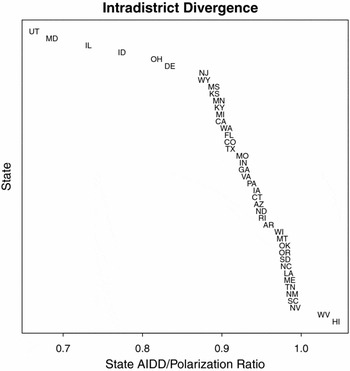
The right-hand side of this equation is the average intradistrict divergence between the parties. We abbreviate it as {AIDD}. When there is positive sorting such that more conservative districts are more likely to elect Republicans, then E(x|R) − E(x|D) > AIDD with the difference attributable to sorting. Thus, we can decompose polarization into AIDD and sorting effects. In making cross-state comparisons, however, we will use the ratio of AIDD to total polarization, which captures the amount of polarization that can be attributed to divergence.
Like McCarty, Poole, and Rosenthal (Reference McCarty, Poole and Rosenthal2009), we estimate using matching estimatorsFootnote 23 as well as OLS with interactions between the covariates and party indicators (Wooldridge Reference Wooldridge2002). Our covariate vector z includes presidential vote, median family income, the poverty rate, the percentage of African-Americans and Hispanics, the percentage of college graduates, and the percentage of renters. Because Nebraska is nonpartisan, its legislature is excluded from our analysis. Moreover, data problems in linking presidential election returns to state legislative districts made it difficult to include Massachusetts, New Hampshire, and Vermont. We estimate state fixed effects in the OLS models and match on state in the matching estimates. Although the two techniques produced similar results for the U.S. House, we find that the OLS generally produces larger, but less precise, estimates than matching on our data. So we focus on those from matching.
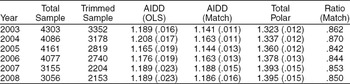
Table 2 reports annual estimates of AIDD for state lower houses. To eliminate concerns about the effects of including districts that are highly unlikely to elect a Democrat or a Republican, we use an algorithm proposed by Crump et al. (Reference Crump, Hotz, Imbens and Mitnick2006) to eliminate districts that have a very high or very low estimated propensity to elect a Republican. The size of this “trimmed” sample is given in column [3]. Columns [4] and [5] present the estimates of AIDD from OLS and matching. Standard errors of these estimates are in parentheses. In column [6], we report an overall measure of polarization of state lower houses. This is estimated from a regression of the NPAT score on party with state fixed effects.
Divergence and Sorting by Year for State Lower Houses
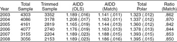
Two features of Table 2 are noteworthy. First, just as McCarty, Poole, and Rosenthal (Reference McCarty, Poole and Rosenthal2009) found, the bulk of polarization is generated by intradistrict divergence. The sorting effect is much smaller in magnitude. By way of comparison, McCarty, Poole, and Rosenthal (Reference McCarty, Poole and Rosenthal2009) find that the ratio of AIDD (estimated by matching) to total polarization was 0.79 for the 108th House. So AIDD accounts for a much larger proportion of state legislative polarization than it does of congressional polarization. Second, although polarization appears to have grown at the state level, the ratio of divergence has grown at about the same rate. Thus, sorting does not appear to account for the increase.Footnote 24
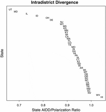
Figure 19 presents the ratio of AIDD and total polarization (difference in means) for each state lower house in our sample.Footnote 25 As we noted previously, there is much variation in the degree of polarization across states. Of interest here is the extent to which the form of polarization (divergence versus sorting) varies across states. Two states (Hawaii and West Virginia) appear to have “negative” sorting – Republicans represent slightly more liberal districts than Democrats.Footnote 26 And sorting is an extremely large contributor to polarization in some others such as Utah and Maryland. In future work we hope to sort out the political, institutional, and socioeconomic factors that lead to the different forms of polarization in different states.
Ratio of Divergence to Polarization for State Lower Houses
Ideology and Parties
Wright and Schaffner (Reference Wright and Schaffner2002) compare roll call voting in Nebraska's nonpartisan legislature with that in Kansas to assess the role of political parties in structuring voting behavior. They found that, relative to Kansas, roll call voting in Nebraska was unusually unstructured and chaotic, characterized by a poorly fitting multidimensional ideological structure and low chamber polarization. They ascribed this difference to the nonpartisan structure in Nebraska, claiming that it is “parties [that] produce the ideological low-dimensional space as a by-product of their efforts to win office. Where the parties are not active in the legislature—Nebraska is our test case—the clear structure found in partisan legislatures disappears.”
But with our results for all 50 states, we are better positioned to assess the degree to which roll call voting behavior in Nebraska is anomalous. When we pool the state's APRE statistic for the first dimension, we find that it is indeed relatively low at 27%.Footnote 27 However, four other states (Arkansas, Louisiana, West Virginia, and Wyoming) score lower on this measure of fit. Similar results hold for a two-dimensional model.
We can also use a party-free measure of polarization—the average ideological distance between members—to compare Nebraska with other states. Just like many other states, Nebraska is polarized, and becoming more so. On the average, Nebraska's Senate is more polarized than 19 other chambers. In fact, it is actually polarizing faster than 71 other chambers over 1996–2008.
CONCLUSION
American state legislatures are an important laboratory for evaluating theories of legislative and electoral institutions. Although key features of the political environment are constant across states, there is sufficient variation in voter preferences and institutions to gain analytical leverage in tests of key hypotheses.
Unfortunately, many of the theories that political scientists would like to bring to this laboratory, especially those based on the spatial model of politics, require estimates of legislator preferences and ideologies. Although the lack of estimates has been overcome in a few specific studies, systematic estimates of state legislative preferences across states over time remains a hindrance. We hope that our data on state legislative preferences will provide the foundation for important breakthroughs in the study of legislative and electoral politics.
Beyond the methodological breakthrough, our article makes a substantive contribution by documenting many key regularities of party positioning and ideological conflict in the American states. First, despite strong nationalizing trends in American politics, political parties below the national level are quite heterogeneous. Although no Republicans in Congress are more liberal than the most conservative Democrats, we find that many states have Republican state legislative contingents that are more liberal than the Democratic caucuses of many states. Moderate partisans thrive at the state level, just as they languish at the national level. Second, although the low stakes, salience, and information in many state legislative elections would point to a lack of ideological responsiveness, we find that this appears not to be the case. In the aggregate, state legislative medians correlate highly with voter ideology measures. Party medians correlate with the preferences of moderates. At a more disaggregated level, the ideal points of state legislators correlate highly with presidential vote in their districts. How legislative responsiveness can subsist in such inhospitable environments is a key question for future research. Finally, we are the first to systematically measure legislative polarization at the state level. At the aggregate level, the states appear to follow the national pattern of high and growing polarization. Like the U.S. Congress, polarization is primarily a manifestation of the different ways Democrats and Republicans represent similar districts, not how voters are sorted across districts. But this aggregate picture misses a lot of important variation in the level, trend, and form of polarization across states. Sorting out the sources of this variation will be the objective of future research.






Comments
No Comments have been published for this article.