





1. Introduction
Dust storms pose a unique opportunity to study particle-laden turbulent flows at extremely high-Reynolds numbers. Several physical mechanisms, including cleavage/fractoelectrification, bombardment charging, pyroelectrification, piezoelectrification, polarisation by Earth’s atmospheric electric field, triboelectrification and contact electrification (Kanagy & Mann Reference Kanagy and Mann1994; Zheng Reference Zheng2013), are believed to cause dust particles to acquire a substantial charge, thereby generating electric fields with intensities exceeding
 $100$
kV m
 $^{-1}$
(e.g. Rudge Reference Rudge1913; Stow Reference Stow1969; Schmidt, Schmidt & Dent Reference Schmidt, Schmidt and Dent1998; Shinbrot & Herrmann Reference Shinbrot and Herrmann2008; Williams et al. Reference Williams, Nathou, Hicks, Pontikis, Russell, Miller and Bartholomew2009; Zhang & Zhou Reference Zhang and Zhou2020; Rahman, Cheng & Samtaney Reference Rahman, Cheng and Samtaney2021). Consequently, in addition to the particle–turbulence couplings in ordinary particle–laden turbulent flows, particle–electrostatics couplings also play a crucial role (e.g. Zheng, Huang & Zhou Reference Zheng, Huang and Zhou2003; Lu et al. Reference Lu, Nordsiek, Saw and Shaw2010; Karnik & Shrimpton Reference Karnik and Shrimpton2012; Zheng Reference Zheng2013; Grosshans & Papalexandris Reference Grosshans and Papalexandris2017; Zhang, Cui & Zheng Reference Zhang, Cui and Zheng2023).
Depending on the flow characteristic parameters, turbulence–particle–electrostatics couplings can be categorised into several regimes. Concerning turbulence–particle couplings, when the particle mass loading is low, the influence of particles on turbulence can be disregarded, which is referred to as a one-way coupling regime. When the particle mass loading is high and the volume fraction is small, turbulence is significantly affected by particles, which is referred to as a two-way coupling regime. When both the mass loading and volume fraction of particles are high enough, particle collisions occur, forming a four-way coupling regime (Elghobashi Reference Elghobashi1994; Balachandar & Eaton Reference Balachandar and Eaton2010; Brandt & Coletti Reference Brandt and Coletti2022). Regarding particle–electrostatics couplings, when the electrostatic Stokes number of particles is small (or large), particle dynamics is dominated by the inertial (or electrostatic) effects of particles (Grosshans et al. Reference Grosshans, Bissinger, Calero and Papalexandris2021; Boutsikakis, Fede & Simonin Reference Boutsikakis, Fede and Simonin2022; Zhang et al. Reference Zhang, Cui and Zheng2023). In dust storms, the dust concentration decreases exponentially with height (McGowan & Clark Reference McGowan and Clark2008; Zheng Reference Zheng2009). As a result, the mass loading of particles is low at locations far from the wall, allowing the turbulence modulation by particles to be neglected. In contrast, close to the wall, both the mass loading and electrostatic Stokes number of particles are large, indicating a strong turbulence–particle–electrostatics coupling (Zhang & Zhou Reference Zhang and Zhou2023), which warrants special attention. It is widely recognised that such strong multifield couplings have pronounced effects on particle transport and aggregation (Lu et al. Reference Lu, Nordsiek, Saw and Shaw2010; Karnik & Shrimpton Reference Karnik and Shrimpton2012; Lu & Shaw Reference Lu and Shaw2015; Boutsikakis et al. Reference Boutsikakis, Fede and Simonin2022; Zhang et al. Reference Zhang, Cui and Zheng2023; Ruan, Gorman & Ni Reference Ruan, Gorman and Ni2024), turbulence modulation (Cui, Zhang & Zheng Reference Cui, Zhang and Zheng2024), the charging properties of particles (Grosshans & Papalexandris Reference Grosshans and Papalexandris2017; Jantač & Grosshans Reference Jantač and Grosshans2024) and the formation of turbulent electric fields (Di Renzo & Urzay Reference Di Renzo and Urzay2018).
One of the major characteristics of dust storms is the significant small-scale intermittency in multiple fields, including wind velocity, the mass concentration of dust particles smaller than 10
 $\unicode {x03BC}$
m (hereafter, PM10 dust concentration) and electric field (Zhang, Tan & Zheng Reference Zhang, Tan and Zheng2023). Intuitively, the time series of these fields displays intense sporadic local fluctuations. Statistically, the probability density function of the increments in these fields deviates increasingly from the Gaussian distribution as the scale decreases (i.e. the flatness increases and exceeds three with decreasing scale), and the high-order structure functions deviate from Kolmogorov linear scaling. Compared to clean-air conditions, the intermittency of wind velocity in dust storms is significantly enhanced at small scales, while it remains largely unchanged at large scales. This may be due to high concentrations of dust particles injecting velocity fluctuations at small scales in the near-surface region (Horwitz & Mani Reference Horwitz and Mani2020). Notably, at 5 m above the surface, the intermittency of PM10 dust concentration is the strongest in dust storms, followed by the electric field, with wind velocity showing the least intermittency. In short, compared with the traditional Fourier transform, the wavelet analysis is more suitable for analysing multifield data series recorded in dust storms. This is because the Fourier transform analyses the entire time series globally and provides characteristics in a time-averaged sense, while the wavelet transform provides both time and frequency information (e.g. Meneveau Reference Meneveau1991; Daubechies Reference Daubechies1992; Farge Reference Farge1992; Camussi & Guj Reference Camussi and Guj1997; Torrence & Compo Reference Torrence and Compo1998; Zhou Reference Zhou2021), effectively extracting and characterising intermittent events.
Previous studies have focused on utilising cospectral analysis to investigate the time-averaged linear coupling behaviour in dust storms. For instance, Wang, Zheng & Tao (Reference Wang, Zheng and Tao2017) performed cospectral analysis between the PM10 dust concentration and wind velocity during dust storms. Their findings indicated that low-speed very large-scale motions (VLSMs) reduce the upward flux of PM10 in the logarithmic layer, while high-speed VLSMs enhance the downstream and upward transport of PM10 in higher regions. Subsequently, Zhang & Liu (Reference Zhang and Liu2023) examined the influence of electric fields on dust transport in dust storms using the cospectrum between PM10 dust concentration and electric field. The results demonstrated that electric fields significantly promote PM10 transport at the kilometer-sized synoptic scale, have a secondary inhibitory effect at the hectometer-sized VLSM scale, and exhibit negligible effects at the decameter-sized turbulent integral scale. Similarly, in wind-tunnel blowing snow experiments, Paterna, Crivelli & Lehning (Reference Paterna, Crivelli and Lehning2016) analysed the cospectrum between measured wind velocity and particle mass flux to explore the effects of turbulence on snow particle entrainment. They identified two regimes of snow particle saltation: (a) a turbulence-dependent regime, where turbulence directly regulates weak saltation; (b) a turbulence-independent regime, where strong saltation develops its own length scale independent of turbulence forcing. Besides linear coupling, various phenomena such as the transition to turbulence, transitions from one turbulence regime to another (Monsalve et al. Reference Monsalve, Brunet, Gallet and Cortet2020) and energy transfer between different spectral components (Ritz & Powers Reference Ritz and Powers1986) can be explained only by the nonlinearity of turbulent flows. Bispectral analysis, as introduced by Hasselmann, Munk & MacDonald (Reference Hasselmann, Munk and MacDonald1963) is an effective method to evaluate quadratic phase coupling in the frequency triad
 $f_1$
,
 $f_2$
and
 $f_1+f_2$
. Note that quadratic phase coupling is also referred to as three-wave coupling or triadic interactions in the literature (see e.g. Agnon & Sheremet Reference Agnon and Sheremet1997; Xu et al. Reference Xu, Wan, Song and Li2003; Biferale, Musacchio & Toschi Reference Biferale, Musacchio and Toschi2012; Monsalve et al. Reference Monsalve, Brunet, Gallet and Cortet2020). Strong quadratic coupling processes have been shown to be responsible for spectral energy redistribution (e.g. Elgar & Guza Reference Elgar and Guza1985; Ritz & Powers Reference Ritz and Powers1986; Dudok de Wit & Krasnosel’skikh Reference Dudok de Wit and Krasnosel’Skikh1995), leading to a smoother (Bountin, Shiplyuk & Maslov Reference Bountin, Shiplyuk and Maslov2008) or broader (Unnikrishnan & Gaitonde Reference Unnikrishnan and Gaitonde2020) power spectral density (PSD). Despite its paramount importance, bispectral characteristics in dust storms, especially for PM10 concentration and electric field, have not been explored previously.
In the aforementioned time-averaged coupling analysis, an implicit assumption is that coupling behaviour remains uniform over time. However, owing to the intrinsic intermittency of the various interacting fields in dust storms, it is reasonable to anticipate that both linear and quadratic nonlinear couplings exhibit intermittent behaviour across both temporal and scale domains. In particular, coherent structures, which are highly localised in time and scale (Camussi & Guj Reference Camussi and Guj1997; Camussi et al. Reference Camussi, Grilliat, Caputi-Gennaro and Jacob2010), give rise to short-lived, sporadic coupling between turbulent fields (Camussi, Robert & Jacob Reference Camussi, Robert and Jacob2008; Bernardini et al. Reference Bernardini, Della Posta, Salvadore and Martelli2023) and are known to contribute significantly to the transport of heat, mass, and momentum (Marusic et al. Reference Marusic, McKeon, Monkewitz, Nagib, Smits and Sreenivasan2010). In this regard, while time-averaged coupling analysis has provided valuable insights into certain multifield interactions in dust storms, this framework is inherently limited in its capacity to capture the critical intermittent coupling dynamics that play a crucial role in these processes.
To elucidate the localised linear and nonlinear coupling characteristics of multiple fields in dust storms, we conducted a series of simultaneous measurements of three-dimensional wind velocity, PM10 dust concentration and electric field at a height of 0.9 m above the surface at the Qingtu Lake Observation Array in 2021. At this measurement height, the particle-to-air mass loading ratio and particle electrostatic Stokes number reached the order of 0.1, indicating significant particle–turbulence and particle–electrostatics couplings. Instead of using a Fourier-based data analysis framework, we adopt a wavelet conditional averaging method based on the local intermittency measure, supplemented by wavelet coherence and bicoherence analyses, to evaluate the multifield localised linear and quadratic nonlinear coupling behaviours.
The remainder of this article is organised as follows: In
 $\S$
2, we provide detailed information on the 2021 field measurement set-up and the selected high-fidelity dataset. In
 $\S$
3, we describe the wavelet-based multiple field coupling analysis methods used in this study. The local intermittency, linear coupling and quadratic nonlinear coupling behaviours of multiple fields in dust storms are examined and discussed in detail in
 $\S$
 $\S$
4.1–4.4, respectively. Finally, we summarise the main conclusions of this article in
 $\S$
5.
2. Dataset
2.1. Measurement set-up
Field measurements were conducted from April to June 2021 at the Qingtu Lake Observation Array (QLOA), an atmospheric surface layer turbulence observatory situated between the Badain Jaran Desert and Tengger Desert in China. The dry lake bed of Qingtu Lake, which spans a flat surface covering approximately 20 km
 $^2$
, is devoid of roughness elements such as rocks, vegetation and sand dunes. This extensive flat surface ensures that the atmospheric surface-layer flows at the QLOA site can be considered analogous to the canonical turbulent boundary layers over flat plates after performing standard data quality control procedures (see below) (Hutchins & Marusic Reference Hutchins and Marusic2007; Hutchins et al. Reference Hutchins, Chauhan, Marusic, Monty and Klewicki2012). From April to June, the QLOA site experiences frequent dust storms due to Mongolian cyclones accompanied by strong northwesterly surface winds (Zheng Reference Zheng2009), offering an excellent opportunity to study randomly occurring dust storms.
The three-dimensional wind velocity components, denoted by
 $U$
,
 $V$
and
 $W$
for the streamwise, spanwise and wall-normal directions respectively, along with the ambient temperature (
 $\varTheta$
), were measured at heights of
 $z = \{0.5, 0.9, 1.5, 2.5, 3.49, 5, 7.15, 10.24, 14.65, 20.96, 30\}$
m above the surface. Simultaneously, the PM10 dust concentration (
 $C$
) and electric field (
 $E$
) were recorded at a height of 0.9 m. Additionally, the size distribution of total airborne dust particles was determined by analysing the particle sample collected at 0.9 m height (Microtrac S3500 tri-laser particle size analyzer, Verder Scientific). At this measurement height, the total particle concentration is sufficiently high to bring about strong turbulence–particle–electrostatics couplings, yet it avoids reaching excessively high particle concentrations that could cause the measurement instruments to cease functioning. Throughout this article, the fluctuating components of the measured physical quantities are represented by lowercase letters
 $u$
,
 $v$
,
 $w$
,
 $\theta$
,
 $c$
and
 $e$
. The wind velocities and ambient temperatures were recorded using sonic anemometers (CSAT3B, Campbell Scientific), PM10 dust concentration was measured using a DustTrak II Aerosol Monitor (Model 8530EP, TSI Incorporated), and the electric field was monitored using an electric field mill (CS110, Campbell Scientific). In addition to the size distribution of total airborne dust particles, all other physical quantities were monitored in real-time. The sampling frequency of CSAT3B is 50 Hz, while that of 8530EP and CS110 is 1 Hz. All instruments were factory calibrated to meet the following specifications: the offset error of the CSAT3B was less than
 $\pm$
8 cm s
 $^{-1}$
; the zero drift of the 8530EP was within
 $\pm$
0.002 kg m
 $^{-3}$
over 24 hours; and the accuracy of the CS110 was
 $\pm$
5 % of the reading, with a maximum offset of 8 V m
 $^{-1}$
.
2.2. Dataset description
Since atmospheric flows are uncontrolled, we need to perform a series of rigorous quality control procedures on the observed data to obtain high-fidelity usable data. Firstly, the continuous observations of multiple fields over two months were divided into a series of one-hour datasets. Subsequently, stationarity and stratification stability parameters were calculated for each one-hour dataset. The stationarity of a time series was assessed using the relative non-stationarity parameter (
 $RNP$
), which is defined as the relative difference between the variance of the entire time series and the mean variance of its 12 contiguous 5-minute subsequences. A time series is considered broadly stationary if
 $RNP \leqslant 0.3$
(Foken & Wichura Reference Foken and Wichura1996), and such series were used for the subsequent data analysis in this study. Notably, a time series is regarded as strongly stationary if all possible moments and joint moments remain invariant over time (Bendat & Piersol Reference Bendat and Piersol2011). However, for atmospheric surface layer data, achieving strong stationarity is challenging due to diurnal variations (synoptic scale) and the limited occurrence of neutral stability conditions (Hutchins & Marusic Reference Hutchins and Marusic2007).
The stratification stability of the wind flow was evaluated using the Monin–Obukhov stability parameter,
 $z/L$
. Here,
 $L = -\langle \varTheta \rangle _t u_\tau ^3/(\kappa g (\langle w \theta \rangle _t)_0)$
is the Obukhov length,
 $\kappa = 0.41$
is the von Kármán constant,
 $g = 9.81$
m s
 $^{-2}$
is gravitational acceleration, and
 $(\langle w \theta \rangle _t)_0$
represents the surface heat flux. As done in numerous previous studies (e.g. Klewicki, Priyadarshana & Metzger Reference Klewicki, Priyadarshana and Metzger2008; Hutchins et al. Reference Hutchins, Chauhan, Marusic, Monty and Klewicki2012; Chowdhuri, Kumar & Banerjee Reference Chowdhuri, Kumar and Banerjee2020), the friction velocity was calculated as
 $u_\tau = (\langle u w \rangle _t^2 + \langle v w \rangle _t^2)^{1/4}$
at
 $z = 1.5\,\rm m$
. When
 $|z/L| \leqslant 0.1$
, the wind flow is approximately neutrally stratified, and thermal buoyancy effects are negligible (Kunkel & Marusic Reference Kunkel and Marusic2006).
Following the aforementioned data quality control procedures, nine sets of high-fidelity one-hour data were selected for analysis in this study, consisting of eight dust storm datasets and one clean-air dataset. The main parameters of these datasets are outlined in table 1. For the clean-air dataset, the mean electric field was negative (i.e. downward-pointing) with a magnitude of approximately
 $0.21$
kV m
 $^{-1}$
. In contrast, during dust storms, the mean electric field was positive (i.e. upward-pointing) and reached magnitudes of several tens of kilovolts per meter, indicating intense electrical activity.
Overview of the used one-hour datasets. Here, ‘0428/14–15’ (similarity for others) denotes this dataset was taken on April 28, 2021 at 14: 00–15:00 UTC + 8,
 $U_c= \langle U \rangle _t$
is the convection velocity,
 $u_\tau$
is the friction velocity,
 $\langle \varTheta \rangle _t$
is the mean ambient temperature,
 $\langle C \rangle _t$
is the mean PM10 dust concentration,
 $\langle E \rangle _t$
is the mean electric field,
 $RNP$
is the relative non-stationarity parameter of the streamwise wind velocity,
 $z/L$
is the Monin–Obukhov stability parameter of the wind flow,
 $\varPhi _m$
is the particle-to-air mass loading ratio,
 $\overline {St_{el}}$
is the mean electrostatic Stokes number, and
 $St^+$
is the viscous Stokes number of the 10-
 $\unicode {x03BC}$
m-diameter dust particles.

Furthermore, the particle-to-air mass loading ratio (
 $\varPhi _m$
) and the mean electrostatic Stokes number (
 $\overline {St_{el}}$
) are used to quantify the importance of particle–turbulence and particle–electrostatics couplings, respectively, while the viscous Stokes number (
 $St^+$
) is employed to assess the particle inertial effects. First, the particle-to-air mass loading ratio is defined as
 $\varPhi _m = \rho _p / \rho _f \phi _V$
, where
 $\rho _p$
,
 $\rho _f$
, and
 $\phi _V$
represent the particle mass density, air mass density, and particle volume fraction, respectively. It is well established that turbulence modulation by particles intensifies with increasing
 $\varPhi _m$
, becoming prominent at
 $\varPhi _m \sim O(0.1)$
(e.g. Kulick, Fessler & Eaton Reference Kulick, Fessler and Eaton1994; Yousefi et al. Reference Yousefi, Costa, Picano and Brandt2023). Second, the electrostatic Stokes number is defined as the ratio of the particle relaxation time scale,
 $\tau _p = d_p^2 \rho _p / (18 \nu \rho _f)$
(Maxey Reference Maxey1987; Eaton & Fessler Reference Eaton and Fessler1994), to the characteristic time scale of electrostatic interactions,
 $\tau _{el} = (6\pi \varepsilon _0 m_p / (n q^2))^{1/2}$
(Boutsikakis et al. Reference Boutsikakis, Fede and Simonin2022), expressed as
 $St_{el} = \tau _p / \tau _{el}$
. Here,
 $d_p$
,
 $\nu$
,
 $\varepsilon _0$
,
 $m_p$
,
 $n$
and
 $q$
denote the particle diameter, air kinematic viscosity, vacuum permittivity, particle mass, particle number density, and particle electric charge, respectively. The definition of
 $\tau _{el}$
is derived through dimensional analysis, assuming that
 $\tau _{el}$
is solely determined by
 $\varepsilon _0$
,
 $m_p$
,
 $n$
and
 $q$
. Thus, the electrostatic Stokes number quantifies the relative importance of particle inertia compared to electrostatic forces: inter-particle electrostatic forces are negligible when
 $St_{el}$
is very small, whereas these forces dominate particle dynamics when
 $St_{el}$
is large. In this study, the average electrostatic effect among charged particles is characterised by the mean electrostatic Stokes number
 $\overline {St_{el}}$
, taking into account only the particle class with the mean diameter. Third, the effects of particle inertia are evaluated using the viscous Stokes number,
 $St^+ \equiv \tau _p / \tau _\nu$
, where
 $\tau _\nu = \nu / u_\tau ^2$
represents the viscous time scale. Particles with a large
 $St^+$
are expected to exhibit quasi-ballistic behaviour, while those with a small
 $St^+$
tend to closely follow the fluid flow.
The estimation of the particle-to-air mass-loading ratio
 $\varPhi _m$
and electrostatic Stokes number
 $\overline {St_{el}}$
is based on synchronous measurements of wind velocity, PM10 dust concentration and particle size distribution at 0.9 m height. Herein, several particle properties are used: (a) particle mass density is assumed to be 2650 kg m
 $^{-3}$
, (b) the density and kinematic viscosity of the air are taken as 1.20 kg m
 $^{-3}$
and 1.57
 $\times$
10
 $^{-5}$
m
 $^2$
s
 $^{-1}$
, respectively, and (c) the charge-to-mass ratio of particles is considered to have a typical value of 60
 $\unicode {x03BC}$
C kg
 $^{-1}$
measured in dust storms (Schmidt et al. Reference Schmidt, Schmidt and Dent1998; Zheng, Huang & Zhou Reference Zheng, Huang and Zhou2003), although it may vary slightly from storm to storm. Further details regarding the estimation of
 $\varPhi _m$
and
 $\overline {St_{el}}$
can be found in our previous study (Zhang & Zhou Reference Zhang and Zhou2023). Figure 1 displays an example of the complete time series of the multiple fields in dataset II. It is shown that the multiple fields, particularly PM10 dust concentration and electric field, exhibit significant local intermittent behaviour, posing new demands on data processing methods, which is discussed in
 $\S$
3.
The complete data series of the dataset II. Panels (a–f) correspond to the streamwise (
 $U$
), spanwise (
 $V$
) and wall-normal (
 $W$
) components of the wind velocity, ambient temperature (
 $\varTheta$
), PM10 dust concentration (
 $C$
), as well as electric field (
 $E$
), respectively.

3. Data analysis
3.1. Wavelet transform and wavelet PSD
Classical Fourier analysis represents data as a sum of trigonometric functions that extend to infinity, making it inefficient for dealing with local abrupt changes in multifield time series recorded in dust storms. In contrast, the use of a set of localised basis functions in wavelet transform allows us to unfold time series into the time and scale (or frequency) domain and, therefore, can uncover local intermittent events effectively (Daubechies Reference Daubechies1992; Farge Reference Farge1992; Torrence & Compo Reference Torrence and Compo1998; Zhou Reference Zhou2021). The continuous wavelet transform of a time series
 $\{x(t), \ t=0,\ldots ,N-1\}$
is defined as the convolution of
 $\{x(t)\}$
with a scaled and translated Morlet wavelet (Daubechies Reference Daubechies1992; Torrence & Compo Reference Torrence and Compo1998),
 \begin{align} W_{x}(t,\tau )=\sum _{t'=0}^{N-1}\sqrt {\frac {\delta _t}{\tau }}x(t')\overline {\psi _0}\left [ \frac {(t'-t)\delta _t}{\tau } \right ], \end{align}
where
 $t$
is the localised time index,
 $\tau$
is the wavelet scale that is inversely proportional to frequency
 $f$
(i.e.
 $1/\tau =1.03f$
, see Torrence & Compo (Reference Torrence and Compo1998) for the details), Morlet wavelet is expressed as
 $\psi _0(\eta )=\pi ^{-1/4}e^{(i\omega _0\eta -\eta ^2/2)}$
with dimensionless frequency
 $\omega _0=6$
satisfying the admissibility condition,
 $\overline {()}$
denotes the complex conjugate, and
 $\delta _t$
is the sampling interval of the time series
 $\{x(t)\}$
. Here, the discrete scales
 $\{\tau (j)\}$
are selected as fractional powers of two:
 \begin{align} \tau (j) & =\tau _02^{j\delta _j}, \quad j=0,1,\ldots ,J, \\[-2pt] \nonumber \end{align}
 \begin{align} J & =\delta _j^{-1}\log _2\left(\frac {N\delta _t}{\tau _0}\right), \\[6pt] \nonumber \end{align}
where
 $\tau _0=2\delta _t$
is the smallest resolvable scale,
 $J$
determines the largest scale, and
 $\delta _j$
is the spacing between discrete scales.
As the square of a wavelet coefficient gives a fluctuating energy at a given time index
 $t$
and scale
 $\tau$
, we thus define the local wavelet PSD of the time series
 $\{x(t)\}$
as (Farge Reference Farge1992; Alexandrova et al. Reference Alexandrova, Carbone, Veltri and Sorriso-Valvo2008; Ruppert-Felsot, Farge & Petitjeans Reference Ruppert-Felsot, Farge and Petitjeans2009)
 \begin{align} \psi _{xx}(t,\tau )=2\delta _t\left |W_{x}(t,\tau )\right |^2. \end{align}
The global wavelet PSD is given by
 \begin{align} \phi _{xx}(\tau ) = \langle \psi _{xx}(t,\tau ) \rangle _t=\frac {1}{N}\sum _{t=0}^{N-1} \psi _{xx}(t,\tau ), \end{align}
where the time average
 $\langle \rangle _t$
is performed over the whole period. It is demonstrated that the global wavelet PSD corresponds to the smoothed Fourier PSD, providing an unbiased and consistent estimation of the true global PSD (Percival Reference Percival1995; Torrence & Compo Reference Torrence and Compo1998).
3.2. Intermittency and coherent signature
Traditionally, the intermittency of a time series
 $\{x(t)\}$
at scale
 $\tau$
can be characterised by the non-Gaussian probability density function (PDF) of the field increment
 $\Delta x(t,\tau )=x(t+\tau )-x(t)$
between two time indexes
 $t$
and
 $t+\tau$
(Frisch Reference Frisch1995; Pope Reference Pope2000). Thanks to the fact that the real part of the wavelet coefficient
 $W_x(t,\tau )$
is proportional to the field increment
 $\Delta x(t,\tau )$
(Bernardini et al. Reference Bernardini, Della Posta, Salvadore and Martelli2023; Zhang et al. Reference Zhang, Tan and Zheng2023), such deviations from the Gaussian PDF can be more conveniently measured by the wavelet flatness factor (Meneveau Reference Meneveau1991; Camussi & Guj Reference Camussi and Guj1997; Alexandrova et al. Reference Alexandrova, Carbone, Veltri and Sorriso-Valvo2008):
 \begin{align} F_{x}(\tau )=\frac {\left \langle \left | W_{x}(t,\tau ) \right | ^4 \right \rangle _t}{\left \langle \left | W_{x}(t,\tau ) \right | ^2 \right \rangle ^2_t}, \end{align}
which quantifies the level of intermittency at scale
 $\tau$
. Notably, a Gaussian PDF corresponds to a wavelet flatness factor with a value of 3.
In contrast to wavelet flatness factor, the so-called local intermittency measure (LIM) (Farge Reference Farge1992; Camussi & Guj Reference Camussi and Guj1997),
 \begin{align} I_{x}(t,\tau )=\frac {\left | W_{x}(t,\tau ) \right | ^2}{\left \langle \left | W_{x}(t,\tau ) \right | ^2 \right \rangle _t }, \end{align}
is defined by the ratio of local energy at the time index
 $t$
and the scale
 $\tau$
to the time-averaged energy at the same scale and is generally used to quantify the level of local intermittency.
Based on LIM, it is convenient to extract time signatures of coherent structures from single-point measurements (Camussi & Guj Reference Camussi and Guj1997; Guj & Camussi Reference Guj and Camussi1999; Camussi et al. Reference Camussi, Grilliat, Caputi-Gennaro and Jacob2010). The basic idea is that intermittency is closely related to the strong field gradients (or field singularity) resulting from the passage of coherent structures. More specifically, the localised energetic coherent structures can be well projected onto a wavelet basis and thus are represented by sparse wavelet coefficients of large modules at a given time and scale (Salem et al. Reference Salem, Mangeney, Bale and Veltri2009; Camussi et al. Reference Camussi, Grilliat, Caputi-Gennaro and Jacob2010). In contrast, the random weak incoherent components have wavelet coefficients extensively spread in the time and scale domain with a considerably smaller module compared to the coherent coefficients. Consequently, a large LIM could be considered as a result of coherent structures passing through the measurement points according to (3.7) (Camussi & Guj Reference Camussi and Guj1997; Guj & Camussi Reference Guj and Camussi1999; Camussi et al. Reference Camussi, Robert and Jacob2008; Salem et al. Reference Salem, Mangeney, Bale and Veltri2009).
To clarify the relationships among the coherent structures of multiple fields in dust storms, a wavelet conditional average method is used to identify the phase-averaged coherent signatures of the wind velocity, PM10 dust concentration and electric field (Camussi & Guj Reference Camussi and Guj1997; Guj & Camussi Reference Guj and Camussi1999; Camussi Reference Camussi2002; Camussi & Di Felice Reference Camussi and Di Felice2006; Camussi et al. Reference Camussi, Robert and Jacob2008; Salem et al. Reference Salem, Mangeney, Bale and Veltri2009; Camussi et al. Reference Camussi, Grilliat, Caputi-Gennaro and Jacob2010; Crawley et al. Reference Crawley, Gefen, Kuo, Samimy and Camussi2018). The coherent signatures of a time series are defined as the portions of the original time series (i.e. time series segments of appropriate width) that are centred around the energetic coherent structures. It is reasonably expected that LIM at scale
 $\tau _s$
larger than a threshold
 $T_h$
are expected to correspond to the energetic coherent structures. Therefore, a set of time indices
 $\{t_0(i), \ i=0,\ldots ,N_e-1\}$
at which the coherent signatures are centred can be determined by
 \begin{align} \{t_0(i)\}=\{t \big | I_x(t,\tau _s)\gt T_h, \ t=0,\ldots ,N-1\}, \end{align}
where
 $N_e$
is the number of the coherent signatures and
 $\tau _s$
is set to be
 $\tau _0$
in order to obtain a better time resolution and statistical convergence of the conditional average (Camussi et al. Reference Camussi, Grilliat, Caputi-Gennaro and Jacob2010). In addition, the threshold LIM must be high enough, but not too high, so that only the most energetic coherent structures are detected and statistical convergence is achieved. A detailed discussion of the selection of threshold LIM
 $T_h$
in the present study is provided in Appendix A. Apparently, a single coherent signature could be either positive or negative, but only positive LIM peaks are selected for identifying energetic signatures in the wavelet conditional average (Crawley et al. Reference Crawley, Gefen, Kuo, Samimy and Camussi2018).
Once the threshold LIM is selected, the
 $i$
th extracted coherent signature
 $\{\widetilde {x}_i(j), j=0,\ldots ,\varXi \}$
can be explicitly expressed as
 \begin{align} \widetilde {x}_i(j)=x(t_0(i)-\varXi /2+j), \end{align}
where
 $\varXi +1$
is the width of each extracted coherent signature.
The resulting phase-averaged coherent signature of time series
 $\{x(t)\}$
is accordingly written as
 \begin{align} \langle \widetilde {x} \rangle = \langle \widetilde {x}_i(j) \rangle _{N_e} = \frac {1}{N_e}\sum _{i=0}^{N_e-1}\widetilde {x}_i(j), \end{align}
where
 $j=0,\ldots ,\varXi$
and the ensemble average
 $\langle \rangle _{N_e}$
is taken over all extracted coherent signatures centred at
 $\{t_0(i)\}$
. It is clear that the averaged coherent signature
 $\langle \widetilde {x} \rangle$
represents the pattern of the most energetic coherent structures hidden in the original time series.
3.3. Wavelet coherence and linear coupling
To quantitatively assess the correlation between two time series
 $\{x(t)\}$
and
 $\{y(t)\}$
, the cross wavelet transform
 $W_{xy}$
can be introduced as (Hudgins, Friehe & Mayer Reference Hudgins, Friehe and Mayer1993)
 \begin{align} W_{xy}(t,\tau )=W_{x}(t,\tau )\overline {W_{y}}(t,\tau ). \end{align}
In analogy with the Pearson correlation coefficient, the wavelet coherence between two time series
 $\{x(t)\}$
and
 $\{y(t)\}$
is given by (Grinsted, Moore & Jevrejeva Reference Grinsted, Moore and Jevrejeva2004; Camussi et al. Reference Camussi, Robert and Jacob2008)
 \begin{align} \gamma _{xy}^{2}(t,\tau )=\frac {\left |\mathcal {S}\left ( W_{xy}(t,\tau )\right )\right |^{2}}{\mathcal {S}\left (\left |W_{x}(t,\tau )\right |^{2}\right ) \mathcal {S}\left (|W_{y}(t,\tau )|^{2}\right )}, \end{align}
where
 $\mathcal {S}$
is a smoothing operator in time and scale domain and can be used to build a balance between desired time and scale resolution and statistical significance (Grinsted et al. Reference Grinsted, Moore and Jevrejeva2004). In this study, the smoothing operator is given by
 $\mathcal {S}(W)=\mathcal {S}_{{scale }}(\mathcal {S}_{{time }}(W(t, \tau )))$
, where
 $\mathcal {S}_{{scale }}$
and
 $\mathcal {S}_{{time }}$
denote smoothing along the wavelet scale and time axis, respectively. Following Grinsted et al. (Reference Grinsted, Moore and Jevrejeva2004) and Camussi et al. (Reference Camussi, Robert and Jacob2008), we define the time-axis smoothing as
 $\mathcal {S}_{{time }}(W(t, \tau ))=W(t, \tau ) * c_1 \exp (-t^2/(2 \tau ^2))$
at a fixed
 $\tau$
, and the scale-axis smoothing as
 $\mathcal {S}_{{scale }}(W(t, \tau ))=W(t, \tau ) * c_2 \Pi (0.6 \tau )$
at a fixed
 $t$
. Here, the symbol
 $*$
denotes the convolution product,
 $c_1$
and
 $c_2$
are normalisation constants, and
 $\Pi$
is the rectangle function. The scale smoothing is implemented using a boxcar filter with a width of 0.6. It is obvious that wavelet coherence
 $\gamma _{xy}^{2}(t,\tau )$
ranges from 0 to 1 and can be considered as a localised correlation coefficient in time and scale domain. In a system consisting solely of two interacting time series, wavelet coherence also represents a measure of the localised linear coupling between two time series (Ritz & Powers Reference Ritz and Powers1986; Narayanan & Hussain Reference Narayanan and Hussain1996; Bendat & Piersol Reference Bendat and Piersol2011). When
 $\gamma _{xy}^2(t,\tau )=1$
,
 $\{x(t)\}$
and
 $\{y(t)\}$
are perfectly linearly coupled at time index
 $t$
and scale
 $\tau$
.
It is straightforward to extend the concept of wavelet coherence to the case of multiple interacting time series, for example,
 $\{y(t)\}$
,
 $\{x_1(t)\}$
and
 $\{x_2(t)\}$
. In many situations,
 $\{y(t)\}$
(e.g. PM10 dust concentration) is coupled to both
 $\{x_1(t)\}$
and
 $\{x_2(t)\}$
(e.g. wind velocity and electric field). To uncover the ‘pure’ linear coupling between
 $\{y(t)\}$
and
 $\{x_1(t)\}$
, one can define the partial wavelet coherence analogous to partial correlation as (Mihanović, Orlić & Pasarić Reference Mihanović, Orlić and Pasarić2009; Xiang & Qu Reference Xiang and Qu2018)
 \begin{align} \gamma _{yx_1(x_2)}^2(t,\tau )=\frac {\left |\gamma _{yx_1}(t,\tau )-\gamma _{yx_2}(t,\tau )\overline {\gamma _{x_1x_2}}(t,\tau )\right |^{2}}{ \left ( 1-\gamma _{yx_2}^2(t,\tau ) \right ) \left( 1-\vphantom{\gamma _{yx_2}^2}\gamma _{x_1x_2}^2(t,\tau ) \right ) }, \end{align}
where
 $\gamma _{yx_1}$
(similarly for
 $\gamma _{yx_2}$
and
 $\gamma_{x_1x_2}$
) is given by
 \begin{align} \gamma _{yx_1}(t,\tau )=\frac { \mathcal {S}\left ( W_{yx_1}(t,\tau )\right )}{\mathcal {S}\left (\left |W_{y}(t,\tau )\right |^{2}\right )^{1/2} \mathcal {S}\left (\left |W_{x_1}(t,\tau )\right |^{2}\right )^{1/2}}. \end{align}
Accordingly, partial wavelet coherence
 $\gamma _{yx_1(x_2)}^2$
measures the localised linear coupling between
 $\{y(t)\}$
and
 $\{x_1(t)\}$
after excluding the influence of
 $\{x_2(t)\}$
. Moreover, the multiple wavelet coherence defined by (Mihanović, Orlić & Pasarić Reference Mihanović, Orlić and Pasarić2009),
 \begin{align} \gamma _{yx_1x_2}^2(t,\tau )=\frac {\gamma _{yx_1}^2(t,\tau )+\gamma _{yx_2}^2(t,\tau )-2\text {Re}\left (\gamma _{yx_1}(t,\tau )\overline {\gamma _{yx_2}}(t,\tau )\overline {\gamma _{x_1x_2}}(t,\tau )\right )}{1-\gamma _{x_1x_2}^2(t,\tau )}, \end{align}
can be used to account for the proportion of wavelet power of
 $\{y(t)\}$
at a time index
 $t$
and scale
 $\tau$
explained by the linear relationship with
 $\{x_1(t)\}$
and
 $\{x_2(t)\}$
. In (3.15),
 $\operatorname {Re}()$
denotes the real part of a complex number.
Overall, as opposed to Fourier coherence, wavelet coherence and partial wavelet coherence provides a powerful tool to examine the localised linear coupling between two or three fields.
3.4. Wavelet bicoherence and quadratic nonlinear coupling
Aside from linear coupling, higher-order nonlinear couplings are undoubtedly broadband and significant in turbulent flows. In particular, frequency (or equivalently scale) components can interact with one another, generating new components at their sum (or difference) frequencies, known as combination components. In other words, the phases of the combination components are coupled to the primary interacting frequency pairs. This phenomenon goes by several different names including three-wave coupling, nonlinear triadic interactions and quadratic nonlinear (or phase) coupling but in each case the same basic mechanisms are involved.
Owing to the intermittent nature of turbulent fields, these phase couplings are not entirely filling in the time and frequency/scale space. In contrast to the Fourier bicoherence, which serves as a global phase coupling measure, the wavelet bicoherence can be used to detect the short-lived intermittent quadratic nonlinear coupling (Van Milligen, Hidalgo & Sanchez Reference Van Milligen, Hidalgo and Sanchez1995; Lancaster et al. Reference Lancaster, Iatsenko, Pidde, Ticcinelli and Stefanovska2018). The wavelet auto-bicoherence of time series
 $\{x(t)\}$
over the period
 $t \in [0, \ N-1 ]$
is defined by (Van Milligen et al. Reference Van Milligen, Hidalgo and Sanchez1995; Schulte Reference Schulte2016)
 \begin{align} b^2_{xxx}(\tau _1,\tau _2)=\frac {\left | \sum _{t=0}^{N-1} W_{x}(t,\tau _1)W_{x}(t,\tau _2)\overline {W_{x}}(t,\tau )\right |^2 }{\left ( \sum _{t=0}^{N-1} \left |W_{x}(t,\tau ) \right |^2\right ) \left ( \sum _{t=0}^{N-1} \left |W_{x}(t,\tau _1)W_{x}(t,\tau _2) \right |^2\right )}, \end{align}
where the frequency sum rule,
 \begin{align} \frac {1}{\tau _1}+\frac {1}{\tau _2}=\frac {1}{\tau }, \end{align}
is satisfied. The auto-bicoherence
 $b^2_{xxx}(\tau _1,\tau _2)$
determines the degree of quadratic nonlinear coupling among scales
 $\tau _1$
,
 $\tau _2$
and
 $\tau$
of time series
 $\{x(t)\}$
over the period
 $t\in [0, N-1 ]$
. By definition, wavelet auto-bicoherence is bounded between 0 and 1, with
 $b^2_{xxx}(\tau _1,\tau _2)=0$
for independent random phase relationships, and
 $b^2_{xxx}(\tau _1,\tau _2)=1$
for a maximum amount of coupling.
In turbulent flows, quadratic nonlinear couplings represent the nonlinear energy transfer among turbulent motions at scales
 $\tau _1$
,
 $\tau _2$
and
 $\tau$
, as well as the breakup of vortices (e.g.
 $\tau \rightarrow (\tau _1, \tau _2)$
) and the formation of new vortices (e.g.
 $(\tau _1, \tau _2) \rightarrow \tau$
) (Kim & Williams Reference Kim and Williams2006). These processes ultimately lead to the redistribution of energy across different scales. Consequently, strong quadratic nonlinear couplings are indicative of notable spectral energy redistribution (Elgar & Guza Reference Elgar and Guza1985; Kim & Williams Reference Kim and Williams2006; Bountin et al. Reference Bountin, Shiplyuk and Maslov2008; Unnikrishnan & Gaitonde Reference Unnikrishnan and Gaitonde2020), by means of both nonlinear energy transfer and the generation and disintegration of turbulent structures.
Similarly, the wavelet cross-bicoherence over the period
 $t\in [0, N-1 ]$
can be defined as (Van Milligen et al. Reference Van Milligen, Sanchez, Estrada, Hidalgo, Brañas, Carreras and García1995; Lancaster et al. Reference Lancaster, Iatsenko, Pidde, Ticcinelli and Stefanovska2018)
 \begin{align} b^2_{yxx}(\tau _1,\tau _2)=\frac {\left | \sum _{t=0}^{N-1} W_{x}(t,\tau _1)W_{x}(t,\tau _2)\overline {W_{y}}(t,\tau )\right |^2 }{\left (\sum _{t=0}^{N-1} \left |W_{x}(t,\tau _1)W_{x}(t,\tau _2) \right |^2 \right ) \left ( \sum _{t=0}^{N-1} \left | W_{y}(t,\tau ) \right |^2\right ) }, \end{align}
which measures the degree of quadratic nonlinear coupling in the period
 $ [0, N-1 ]$
among scales
 $\tau _1$
and
 $\tau _2$
of
 $\{x(t)\}$
and scale
 $\tau$
of
 $\{y(t)\}$
.
The wavelet cross-bicoherence can be also extended to the case of three coupled time series
 $\{x_1(t)\}$
,
 $\{x_2(t)\}$
and
 $\{y(t)\}$
(e.g. Corke, Shakib & Nagib Reference Corke, Shakib and Nagib1991; Corke et al. Reference Corke, Arndt, Matlis and Semper2018; Arndt et al. Reference Arndt, Corke, Matlis and Semper2020; Middlebrooks et al. Reference Middlebrooks, Corke, Matlis and Semper2024):
 \begin{align} b^2_{yx_1x_2}(\tau _1,\tau _2)= \frac {\left | \sum _{t=0}^{N-1} W_{x_1}(t,\tau _1)W_{x_2}(t,\tau _2)\overline {W_{y}}(t,\tau )\right |^2 }{\left (\sum _{t=0}^{N-1} \left |W_{x_1}(t,\tau _1)W_{x_2}(t,\tau _2) \right |^2 \right ) \left ( \sum _{t=0}^{N-1} \left | W_{y}(t,\tau ) \right |^2\right ) }, \end{align}
which is a measure the degree of quadratic nonlinear coupling in the period
 $ [0, N-1 ]$
among scale
 $\tau _1$
of
 $\{x_1(t)\}$
, scale
 $\tau _2$
of
 $\{x_2(t)\}$
and scale
 $\tau$
of
 $\{y(t)\}$
. Although the concept of partial wavelet coherence
 $\gamma _{yx_1(x_2)}^2$
mentioned above can be used to extract the ‘pure’ linear coupling between
 $\{y(t)\}$
and
 $\{x_1(t)\}$
(or
 $\{x_2(t)\}$
), we have no similar theory of partial wavelet bicoherence to isolate the ‘pure’ quadratic nonlinear coupling so far (McComas & Briscoe Reference McComas and Briscoe1980; Van Milligen et al. Reference Van Milligen, Hidalgo and Sanchez1995).
Furthermore, the wavelet summed bicoherence is defined as (Van Milligen et al. Reference Van Milligen, Hidalgo and Sanchez1995)
 \begin{align} B^2(\tau )=\frac {\sum b^2(\tau _1,\tau _2)}{\xi (\tau )}, \end{align}
where the sum is taken over all
 $\tau _1$
and
 $\tau _2$
such that (3.17) is satisfied and
 $\xi (\tau )$
is the number of summands in the summation. By essentially aggregating or averaging the quadratic nonlinear couplings over multiple frequency pairs
 $\tau _1$
and
 $\tau _2$
, the summed bicoherence
 $B^2(\tau )$
provides insight into the overall strength or prevalence of the quadratic nonlinear couplings across the entire spectrum. Clearly, a higher summed bicoherence value suggests a stronger quadratic nonlinear coupling between frequency components at specific frequency combinations.
4. Results and discussion
4.1. Strong two-way particle–turbulence and particle–electrostatics couplings
We begin by determining the presence of strong two-way particle–turbulence and particle–electrostatics couplings in the eight dust storm datasets. Since particles are influenced by turbulence and the electric field is generated by moving charged particles, our objective is to explore whether dust particles introduce a significant feedback effect on turbulence and whether the electric field substantially affects particle transport.
First, these significant two-way couplings can be indirectly inferred from the large dimensionless parameters,
 $\varPhi _m$
and
 $\overline {St_{el}}$
. At a height of 0.9 m, both
 $\varPhi _m$
and
 $\overline {St_{el}}$
are estimated to reach approximately
 $O(0.1)$
(see table 1), indicating strong two-way couplings between particle–turbulence and particle–electrostatics, as suggested by the previously established criteria (Elghobashi Reference Elghobashi1994; Boutsikakis et al. Reference Boutsikakis, Fede and Simonin2022; Zhang et al. Reference Zhang, Cui and Zheng2023).
Additionally, direct evidence is provided by examining how dust particles regulate turbulence statistics and how electrostatic effects influence PM10 dust concentration and vertical turbulent flux within a narrow range of friction velocity. Wall-normal profiles of the inner-scaled mean streamwise wind velocity and Reynolds shear stress are presented in figure 2. For comparison, the Reynolds stress documented by Hutchins et al. (Reference Hutchins, Chauhan, Marusic, Monty and Klewicki2012) at the Surface Layer Turbulence and Environmental Science Test facility is also plotted in figure 2(b). Using the boundary layer thickness
 $\delta =166\pm 38$
m at the QLOA site (see Wang & Zheng Reference Wang and Zheng2016) and calculating the kinematic viscosity
 $\nu$
based on Sutherland’s law (Sutherland Reference Sutherland1893), we find that the friction Reynolds number
 $Re_\tau \equiv u_\tau \delta /\nu$
varies from
 $3.44\times 10^6$
to
 $6.72\times 10^6$
for the eight dust storm datasets, which is consistent with the values reported by Hutchins et al. (Reference Hutchins, Chauhan, Marusic, Monty and Klewicki2012). The strong consistency between the results of Hutchins et al. (Reference Hutchins, Chauhan, Marusic, Monty and Klewicki2012) and the clean-air dataset indicates the high quality of the datasets used herein. It is evident that the mean streamwise velocity and Reynolds stress for both clean-air and dust storm datasets fairly follow a logarithmic law. However, compared to the clean-air dataset, the dust storm datasets exhibit lower inner-scaled mean streamwise wind velocity and relatively higher inner-scaled Reynolds stress (especially for
 $y^+ \gtrsim O(10^5)$
), suggesting a substantial feedback effect of dust particles on wind flow (figure 2
b).
(a) Wall-normal profiles of the inner-scaled mean streamwise wind velocity
 $\langle U^+ \rangle=\langle U \rangle/u_\tau$
. (b) Wall-normal profiles of the inner-scaled Reynolds shear stress
 $-\langle u^+ w^+\rangle =-\langle uw\rangle /u_\tau ^2$
: black pentagrams denote the data from Hutchins et al. (Reference Hutchins, Chauhan, Marusic, Monty and Klewicki2012), while other symbols represent current QLOA data.

(a) Dependence of mean PM10 dust concentration on friction wind velocity (
 $u_\tau$
) and electrostatic Stokes number (
 $\overline {St_{el}}$
). (b) Dependence of vertical turbulent dust flux on
 $u_\tau$
and
 $\overline {St_{el}}$
, where the vertical turbulent dust flux
 $\langle cw \rangle _t$
is normalised by the product of friction velocity and the mean PM10 dust concentration from dataset I, denoted as
 $(u_\tau \langle C \rangle _t)_1$
.

On the other hand, figure 3(a,b) illustrate the dependence of mean PM10 dust concentration and vertical turbulent dust flux on friction wind velocity and electrostatic Stokes number for the eight dust storm datasets. Since the friction Reynolds numbers of these data are nearly identical (i.e.
 $u_\tau = 0.53 \pm 0.04$
m s
 $^{-1}$
), the variations in the concentration and vertical turbulent dust flux of the PM10 dust particles are primarily caused by electrostatic effects. A clear increasing trend in mean PM10 dust concentration is observed with respect to the electrostatic Stokes number (figure 3
a), suggesting that inter-particle electrostatic forces facilitate the lifting of particles from sandy surfaces. In addition, figure 3(b) shows both positive (upward) and negative (downward) vertical turbulent dust fluxes, which correspond to the processes of dust dispersal into the air and dust redeposition onto the surface, respectively (Shao Reference Shao2008). In both cases, the magnitude of the vertical turbulent dust flux tends to increase with the electrostatic Stokes number, indicating that electrostatic effects tend to enhance vertical turbulent dust flux. In short, a significant two-way coupling between particles and electrostatics is evident in the analysed datasets.
Autocorrelation functions for the fluctuating streamwise wind velocity, PM10 dust concentration and electric fields. Solid lines represent the mean autocorrelation functions calculated from eight dust storm datasets. The shaded areas indicate the standard deviations of the autocorrelation functions across these datasets.

In addition to the first- and second-order one-point statistics, the two-point longitudinal autocorrelation functions of the fluctuating streamwise wind velocity, PM10 dust concentration and electric fields are calculated as,
 \begin{align} R_{AA}(\Delta x)=\frac {\langle A(x) A(x+\Delta x)\rangle }{\sigma _{A(x)} \sigma _{A(x+\Delta x)}}, \end{align}
where
 $A\in \{u,c,e\}$
and the longitudinal separation
 $\Delta x$
is obtained from the time lag
 $\Delta t$
using Taylor’s hypothesis of frozen turbulence, i.e.
 $\Delta x=\Delta tU_c$
. As shown in figure 4, the autocorrelation functions exhibit long tails, extending to distances of up to approximately 300 m (only the positive part is shown due to symmetry), which is equivalent to twice the boundary layer thickness. These non-zero correlations at large separations indicate the presence of large-scale coherent structures in wind velocity, PM10 dust concentration, and electric fields. The underlying physical mechanism is that if a large structure is present, there will be some degree of correlation between the motions at different points across the boundary layer region that the structure spans. The autocorrelation functions thus provide insight into the average picture of these large-scale coherent structures.
It is important to stress that the existence of large-scale coherent structures in the electric fields suggests conspicuous charge separation on a large scale comparable with boundary-layer thickness, as electric fields are directly related to space charge density according to Coulomb’s law. This large-scale charge separation can be explained by the tendency of smaller, low-inertia, negatively charged particles to accumulate in specific regions of the instantaneous turbulence field (Eaton & Fessler Reference Eaton and Fessler1994), while larger, high-inertia, positively charged particles are distributed more uniformly, as previously reported (Di Renzo & Urzay Reference Di Renzo and Urzay2018; Zhang & Zhou Reference Zhang and Zhou2020).
4.2. Multifield local intermittent behaviour
Wavelet flatness
 $F_x$
of the fluctuating streamwise wind velocity (
 $x=u$
), PM10 dust concentration (
 $x=c$
) and electric field (
 $x=e$
) for datasets from (a) I to (h) VIII.

As previously mentioned, the multiple fields in dust storms exhibit conspicuous intermittent behaviour in the time domain (figure 1), whose time-averaged characteristics can be quantified through wavelet flatness factor. Figure 5 compares the wavelet flatness factor of the streamwise wind velocity, PM10 dust concentration and electric field at various scales for the used eight dust storm datasets (table 1). It can be seen that, at larger scales (i.e.
 $\tau \sim 10^2$
s), the multifield wavelet flatness factor is close to 3, indicating that the PDFs of the multiple field increments obey a Gaussian distribution and the multiple fields are non-intermittent at larger scales. However, as the scale decreases, the multifield wavelet flatness factor increases, suggesting a super-Gaussian PDFs of the field increments and presence of intermittency at smaller scales. Importantly, the wavelet flatness factor of PM10 dust concentration and electric field is nearly identical but greater than that of the streamwise wind velocity, especially at smaller scales. This multifield intermittency behaviour near the surface differs from that far away from the surface, where the intermittency is strongest for PM10 dust concentration, followed by the electric field, and weakest for wind velocity (Zhang et al. Reference Zhang, Tan and Zheng2023).
LIMs of the fluctuating (a) streamwise wind velocity, (b) PM10 dust concentration and (c) electric field for dataset II. The upper region enclosed by the black dashed line and the coordinate axes represents the ‘cone of influence’, where edge effects become significant. The black contour denotes the 95 % confidence level for white noise.

Phase-averaged coherent signatures of the fluctuating streamwise wind velocity (
 $x=u$
), PM10 dust concentration (
 $x=c$
) and electric field (
 $x=e$
) for datasets from (a) I to (h) VIII. The phase-averaged coherent signatures are normalised by the corresponding standard deviations of the original time series
 $\{x(t)\}$
, i.e.
 $\langle \tilde {x} \rangle /\sigma _x$
.

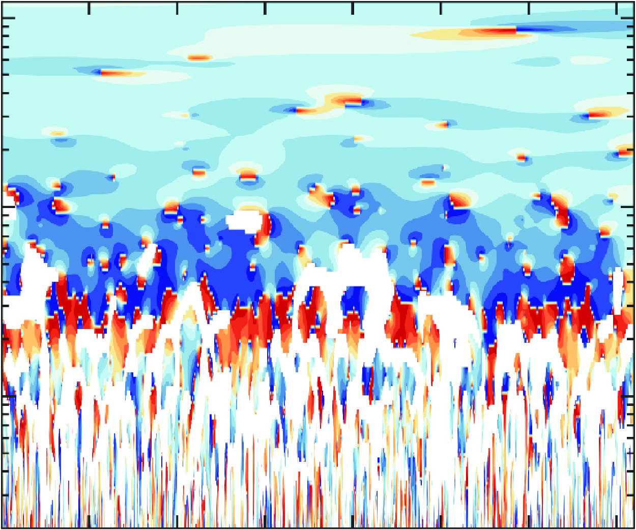
Next, the localised intermittent behaviour for multiple fields is assessed using LIM. As exemplified in figure 6, it depicts the multifield LIM for dataset II. Due to the higher sampling frequency of wind velocity compared to PM10 dust concentration and electric field, the LIM for streamwise wind velocity is presented across broader scales than that for PM10 dust concentration and electric field (i.e.
 $\tau \in [0.04, 2]$
s, corresponding to the shaded area in figure 6(a). It is important to emphasise that the magnitude of the sampling frequency only affects the smallest resolvable scale in the LIM graph but does not change the LIM distribution in the time domain. It is clear that all LIMs do not completely fill the time and scale domain, becoming increasingly fragmented as the scale decreases. Within the entire resolved scale range of one-Hertz data
 $\tau \in [2, 1.5\times 10^3]$
s, the overall LIM patterns for PM10 dust concentration and electric field behave very similarity. At larger scales (i.e.
 $\tau \in [1\times 10^2,1.5\times 10^3]$
s), all LIMs display similar behaviour, particularly showing high values over a broad time window as a result of an energetic synoptic-scale motion passing through the measurement point. However, the LIM for PM10 dust concentration and electric field appears sparser than that for streamwise wind velocity at smaller scales (i.e.
 $\tau \in [2,1\times 10^2]$
s). Similar conclusions can be drawn for other datasets, albeit not presented here for clarity.
To gain further insight, the proposed wavelet conditional average method (i.e. equation (3.8)) is utilised to isolate the phase-averaged coherent signatures of the multiple fields in dust storms. The fundamental principle behind this method is that peaks in the LIM distribution correspond to the passage of energetic structures. Therefore, when the LIM,
 $I(t,\tau _0)$
, exceeds a certain threshold value, it is believed to indicate the presence of energetic coherent structures. It is evident that the selection of the threshold LIM is crucial for extracting coherent signatures. In this study, we set the threshold LIM to 2 (see Appendix A), consistent with previous studies (e.g. Camussi & Guj Reference Camussi and Guj1997). It is worth emphasising that, for the sake of comparing different physical fields, we subsampled the wind velocity data to 1 Hz when extracting coherent signals (hence,
 $\tau _0=2$
s). Figure 7 illustrates the phase-averaged coherent signatures extracted from all datasets, which are normalised with respect to the standard deviation of the original time series. Because only positive LIM peaks were utilised, the phase-averaged coherent signatures are all positive within a 100-second duration and exhibit a ‘
 $\Lambda$
’ shape. Clearly, such ‘
 $\Lambda$
-shaped’ coherent signatures for multiple fields display highly similar temporal characteristics. In particular, the coherent signatures of PM10 dust concentration and electric field are shown to collapse well, but they are stronger than those of the streamwise wind velocity.
An important question that warrants further exploration is why the coherent signatures of PM10 dust concentration and electric fields are more pronounced compared to those of wind velocity. A plausible physical explanation is the presence of multiscale ramp-cliff structures in the time series of PM10 dust concentration and electric fields, which produce stronger gradients and, consequently, increased intermittency. Both time series in figure 1(e,f) clearly exhibit a gradual rise (the ramp) followed by a sharp drop (the cliff). In certain instances, this order reverses, featuring a steep increase followed by a more gradual decline. Together, these two patterns are referred to as ramp-cliff structures (Buaria et al. Reference Buaria, Clay, Sreenivasan and Yeung2021). Their characteristic time scales range from a few seconds to several hundred seconds, displaying typical multiscale behaviour in atmospheric boundary layer flow (Belušié & Mahrt Reference Belušiá and Mahrt2020). To understand the origin of these structures, we examine the transport equation for PM10 dust concentration:
 \begin{align} \frac {\partial C}{\partial t}+U_{p, j} \frac {\partial C}{\partial x_j} =\varGamma _C \frac {\partial ^2 C}{\partial x_j^2}, \end{align}
where
 $ U_{p,j}$
and
 $\varGamma _C$
denote the
 $j$
th (
 $j=1,2,3$
) component of the velocity of the dust particles and the diffusion coefficient, respectively (Warhaft Reference Warhaft2000; Shao Reference Shao2008). In (4.2), when the particle inertia, gravitational settling and electrostatic effects are negligible,
 $U_{p,j}$
can be replaced by the wind velocity
 $U_j$
because the relative particle-fluid velocity becomes zero. Notably, this equation is devoid of a pressure term, indicating that the PM10 dust concentration field undergoes large-scale deformation solely through convective processes. In contrast to the velocity field, the essential local isotropisation and mixing effects of pressure are absent in the PM10 dust concentration field. Consequently, PM10 dust concentration can be expelled from the core regions of vortical structures and accumulate along the periphery or at stagnation points, leading to the formation of ramp-cliff structures (Watanabe & Gotoh Reference Watanabe and Gotoh2004). These structures generate steep gradients associated with intense dissipation, thereby enhancing intermittency. With respect to electric fields, previous studies have also demonstrated a close correspondence between the structures of electric fields and PM10 dust concentration (Di Renzo & Urzay Reference Di Renzo and Urzay2018; Zhang Reference Zhang2024), as electric fields are entirely generated by charged dust particles and are therefore determined by their spatial and temporal distribution. Furthermore, from a structural stability perspective, the most intermittent structures in PM10 dust concentration and electric fields manifest as two-dimensional sheet-like structures (Zhang et al. Reference Zhang, Tan and Zheng2023), which are inherently less stable than the filamentary intermittent structures in the velocity field. Thus, the generation and annihilation of these sheet-like structures occur more frequently, resulting in intense fluctuations in both PM10 dust concentration and electric fields (Chen & Cao Reference Chen and Cao1997).
4.3. Multifield linear coupling
In dust storms, the presence of interactions between particles and turbulence, as well as between particles and electrostatics, indicates that PM10 dust concentration is influenced by both turbulent flows and electric fields. In such cases, the wavelet coherence between PM10 dust concentration and wind velocity (or electric field) cannot represent the ‘pure’ linear coupling relationship between them. In this study, the ‘pure’ linear couplings between two interacting fields are assessed using partial wavelet coherence (i.e. equation (3.13)). Figure 8 displays the partial wavelet coherences
 $\gamma _{cw(e)}^2$
and
 $\gamma _{ce(w)}^2$
for dataset II, along with their time-averaged (i.e.
 $\langle \gamma _{cw(e)}^2 \rangle _t$
and
 $\langle \gamma _{ce(w)}^2 \rangle _t$
) and scale-averaged (i.e.
 $\langle \gamma _{cw(e)}^2 \rangle _{\tau }$
and
 $\langle \gamma _{ce(w)}^2 \rangle _{\tau }$
) values. Here we focus on multifield couplings in the vertical direction, because the distribution of PM10 dust concentration is mainly determined by its vertical transport processes (Zheng Reference Zheng2009; Zhang & Liu Reference Zhang and Liu2023), which is also demonstrated in drifting snow (Paterna et al. Reference Paterna, Crivelli and Lehning2016). Notably,
 $w$
is subsampled to 1 Hz to match the sampling frequency of
 $c$
and
 $e$
. The disparity between the time-averaged wavelet coherence and partial wavelet coherence is discussed in detail in Appendix B.
(a) Scale-averaged partial wavelet coherences
 $\langle \gamma _{cw(e)}^2 \rangle _{\tau }$
for the raw (black solid line), intermittent (orange dashed line) and non-intermittent (blue dotted line) components of dataset II. (b) Partial wavelet coherence between the raw PM10 dust concentration and the vertical wind velocity component
 $\gamma _{cw(e)}^2$
. (c) Time-averaged partial wavelet coherences for the raw (black solid line), intermittent (orange dashed line) and non-intermittent (blue dotted line) components of dataset II. (d–f) Same as (a–c) but for partial wavelet coherences between PM10 dust concentration and electric field. In (b,e), the upper region enclosed by the black dashed line and the coordinate axes represents the ‘cone of influence’, where edge effects become significant. The black contour denotes the 95 % confidence level for white noise.

When
 $\tau \lesssim 30$
s,
 $\gamma _{cw(e)}^2$
and
 $\gamma _{ce(w)}^2$
display elongated, intermittent, strikes along the scale axis (figure 8
b,e). This indicates a broadband and intermittent linear coupling behaviour between PM10 dust concentration and vertical wind velocity, as well as between PM10 dust concentration and electric field. However, when
 $\tau \gtrsim 30$
s,
 $\gamma _{cw(e)}^2$
and
 $\gamma _{ce(w)}^2$
no longer exhibit pronounced intermittent behaviour. While sporadic high linear couplings between PM10 dust concentration and vertical wind velocity occur at larger scales, their linear coupling strength remains weak across most time and scale domains. In contrast, PM10 dust concentration and electric field display very high coupling throughout scales above approximately 200 s. This discrepancy in linear coupling at large scales is further reflected in the time-averaged partial wavelet coherence. From figure 8(c,f), it can be seen that
 $\langle \gamma _{cw(e)}^2 \rangle _t$
and
 $\langle \gamma _{ce(w)}^2 \rangle _t$
are almost identical for
 $\tau \lesssim 10$
s. However, with increasing scale,
 $\langle \gamma _{cw(e)}^2 \rangle _t$
remains constant, while
 $\langle \gamma _{ce(w)}^2 \rangle _t$
rapidly increases, reaching its maximum value at
 $\tau \approx 200$
s.
Phase angle between the intermittent components of (a) PM10 dust concentration and vertical wind velocity, as well as (b) PM10 dust concentration and electric field for dataset II. For clarity, the phase angle is conditioned on wavelet coherence greater than 0.25.

To examine whether multifield intermittency plays an important role in the intermittent linear coupling behaviour, we decompose the raw time series of wind velocity, PM10 dust concentration and electric field into a coherent component and a background incoherent component. We then investigate the partial wavelet coherence and phase angle between these components. Following the approach proposed by Farge and co-workers (e.g. Farge, Pellegrino & Schneider Reference Farge, Pellegrino and Schneider2001; Ruppert-Felsot et al. Reference Ruppert-Felsot, Farge and Petitjeans2009), the decomposition process is as follows: (i) apply a continuous wavelet transform to the raw time series to obtain the wavelet coefficients; (ii) coefficients whose modulus exceeds
 $F$
times their standard deviation at the same scale are regarded as associated with energetic coherent structures and are subsequently used to reconstruct the coherent component through a conditioned inverse wavelet transform. In contrast, the remaining coefficients, with relatively smaller moduli, correspond to the incoherent component. In this study, the threshold value
 $F$
is set to 1, because the resulting scaling exponent of the structure function for the incoherent component fully recovers the Kolmogorov’s self-similarity law (Zhang et al. Reference Zhang, Tan and Zheng2023). Thus, through this procedure, the decomposed coherent and incoherent components are intermittent and non-intermittent, respectively.
Figures 8(a,d) and 8(c,f) compare the scale- and time-averaged partial wavelet coherences of the raw series, as well as intermittent and non-intermittent components for dataset II. It is shown that the scale- and time-averaged partial wavelet coherences of the non-intermittent components remain largely invariant with respect to both time and scale. These values are typically small and exhibit significant discrepancies when compared to those of the raw series. This suggests that the non-intermittent components display a weak, yet noticeable, intermittent multifield linear coupling behaviour across the entire time and scale domains. On the contrary, the scale- and time-averaged partial wavelet coherences of the intermittent components closely match those of the raw series, indicating that the intermittent components dominate the multifield linear coupling behaviour, rather than the non-intermittent components.
Since the coupling behaviour is closely related to the phase angle between two interacting time series, we also present the phase angle between the intermittent components of PM10 dust concentration and vertical wind velocity, as well as between PM10 dust concentration and electric field, in figure 9. The phase angle between time series
 $\{x(t)\}$
and
 $\{y(t)\}$
,
 $\alpha _{xy}$
, is computed as
 \begin{align} \alpha _{xy}=\arctan \left (\frac {\Im (W_{xy})}{\Re (W_{xy})} \right ), \end{align}
where
 $\Im ()$
and
 $\Re ()$
denote the imaginary and real parts of a complex number, respectively.
Throughout the entire time and scale domain of figure 9(a), and for
 $\tau \lesssim 30$
s in figure 9(b), the phase angle is nearly constant across scales but exhibits alternating positive and negative values over time. This behaviour, referred to as a phase-unlocked pattern, corresponding to the weak coupling regions identified in figure 8(c,f). Such a weak and phase-unlocked coupling pattern can be attributed to the high multifield intermittency at small scales (figure 5). High intermittency corresponds to short-lived, sporadic and intense fluctuations, which make it difficult to establish a systematic and organised relationship among different fields. However, for larger scales in figure 9(b) (
 $\tau \gtrsim 100$
s), the phase angle remains nearly constant with scale and time, indicative of perfect ‘phase synchronisation’. In these regions, the linear coupling strength exceeds 0.8. The emergence of strong, phase-locked coupling at larger scales is closely associated with the presence of similar multifield large-scale coherent structures (see figure 4). These identical coherent structures, which are thought to dominate the coupling behaviour, are reasonably expected to produce strong coupling and give rise to phase synchronisation. Note that this positive correlation between coupling strength and phase synchronisation is a well-established feature of chaotic systems (Boccaletti et al. Reference Boccaletti, Kurths, Osipov, Valladares and Zhou2002), and it has now been observed in the complex dust storm turbulence.
(a) Scale-averaged multiple wavelet coherences
 $\langle \gamma _{cwe}^2 \rangle _{t}$
for the raw (black solid line), intermittent (orange dashed line) and non-intermittent (blue dotted line) components of dataset II. (b) Multiple wavelet coherence among the raw PM10 dust concentration, vertical wind velocity and electric field
 $\gamma _{cwe}^2$
. (c) Time-averaged multiple wavelet coherences
 $\langle \gamma _{cwe}^2 \rangle _{t}$
for the raw (black solid line), intermittent (orange dashed line) and non-intermittent (blue dotted line) components. In (b), the upper region enclosed by the black dashed line and the coordinate axes represents the ‘cone of influence’, where edge effects become significant. The black contour denotes the 95 % confidence level for white noise.

Comparison of partial wavelet coherence and multiple wavelet coherence for all eight dust storm datasets. Solid lines denote the mean wavelet coherence, where
 $\langle \rangle _{t}$
denotes average over time. Shaded areas indicate the standard deviations of the time-averaged wavelet coherences across the eight datasets.

Besides the ‘pure’ linear coupling between two interacting fields, the combined contribution of vertical wind velocity and electric field to PM10 dust concentration is explored using multiple wavelet coherence, as presented in figure 10. It is evident that the overall pattern of
 $\gamma _{cwe}^2$
resembles that of
 $\gamma _{ce(w)}^2$
, but with higher time-averaged values (figure 10
b). On average, more than 50 % and 95 % of the power of PM10 dust concentration can be accounted for by the linear relationship with vertical wind velocity and electric field at
 $\tau \lesssim 30$
s and
 $\tau \gtrsim 200$
s, respectively (figure 10
c). Also, multiple wavelet coherence appears to be dominated by the multifield intermittent components.
In addition, a detailed comparison of partial wavelet coherence and multiple wavelet coherence for all eight dust storm datasets is shown in figure 11. It is evident that the differences in time-averaged partial wavelet coherence and multiple wavelet coherence among the eight datasets are considerably small (i.e. very narrow shadowed areas in figure 11). From figures 8 and 11, we conclude that when
 $\tau \lesssim 10$
s, the linear coupling behaviours between PM10 dust concentration and vertical wind velocity
 $\gamma ^2_{cw(e)}$
, as well as between PM10 dust concentration and electric field
 $\gamma ^2_{ce(w)}$
, are similar, displaying broadband and intermittent behaviours. Within this scale range, PM10 dust concentration is jointly influenced by vertical wind velocity and electric field. When
 $\tau \gtrsim 10$
s (especially
 $\gtrsim 100$
s), however, the linear coupling between PM10 dust concentration and electric field
 $\gamma ^2_{ce(w)}$
significantly outweighs that of PM10 dust concentration and vertical wind velocity
 $\gamma ^2_{cw(e)}$
, indicating the dominance of the electric field in influencing PM10 dust concentration. This finding is in agreement with the results presented in figure 3, where PM10 dust concentration and vertical turbulent dust flux increase significantly with the electrostatic Stokes number. Furthermore, the multiple wavelet coherence being smaller than unity suggests that PM10 dust concentration cannot be perfectly explained by linear combined couplings with wind velocity and electric field alone, perhaps indicating a significant role played by nonlinear couplings (Narayanan & Hussain Reference Narayanan and Hussain1996).
4.4. Multifield PSD and quadratic nonlinear coupling
(a) Global wavelet PSDs of the streamwise wind velocity, PM10 dust concentration and electric field, where
 $\phi _{uu}^*(f)=\phi _{uu}(f)/u_\tau ^2$
,
 $\phi _{cc}^*(f)=\phi _{cc}(f)/\langle c^2 \rangle$
and
 $\phi _{ee}^*(f)=\phi _{ee}(f)/\langle e^2 \rangle$
. Lines and shaded areas denote the mean and standard deviations for eight dust storm datasets. (b) Compensated wavelet PSDs of the corresponding multiple fields (standard deviations are not shown), where the horizontal dotted and solid lines represent the frequency ranges of the power-law spectra. Note that,
 $\phi _{cc}(f)$
,
 $\phi _{ee}(f)$
and their compensated spectra are vertically shifted for clarity.

As stated in
 $\S$
3.4, wavelet auto-bicoherence is believed to play a role in spectral energy redistribution. Therefore, we attempted to interpret the multifield global wavelet PSDs through the analysis of wavelet auto-bicoherence. Figure 12 shows the multifield global wavelet PSDs for all eight dust storm datasets. It is clear that the global wavelet PSDs for the eight datasets are nearly collapsed onto a single curve (figure 12
a), suggesting identical spectral characteristics among the different datasets. Although the sampling frequency of PM10 dust concentration and the electric field is much lower than that of wind velocity, the global wavelet PSDs of all physical fields exhibit two distinct spectral regions: they show power laws with exponents of
 $\sim f^{-0.96}$
in the low-frequency region, a break at the intermediate frequencies, and steeper power laws with exponents of
 $\sim f^{-1.5}$
or
 $\sim f^{-1.6}$
in the high-frequency region. The former power law is consistent with the ‘complete similarity’ scaling
 $f^{-1}$
(Nickels et al. Reference Nickels, Marusic, Hafez and Chong2005) and the latter one is in line with the Kolmogorov scaling
 $ f^{-5/3}$
(Kolmogorov Reference Kolmogorov1941). These spectral behaviours are clearly observable in the compensated PSDs (figure 12
b). The
 $f^{-1}$
power law of the streamwise velocity can be derived from the inviscid theory of Perry, Henbest & Chong (Reference Perry and Henbest1986), in which both inner scaling,
 $\phi _{uu}(k_x z)/u_\tau ^2=\phi _{uu}(k_x)/(z u_\tau ^2)=f(k_x z)$
, and outer scaling,
 $ \phi _{uu}(k_x \delta )/u_\tau ^2=\phi _{uu}(k_x)/(\delta u_\tau ^2)=f(k_x \delta )$
, are simultaneously valid in an overlap region (Nickels et al. Reference Nickels, Marusic, Hafez and Chong2005; Hwang, Hutchins & Marusic Reference Hwang, Hutchins and Marusic2022). Here,
 $k_x=2\pi f/U_c$
represents the streamwise wavenumber, and
 $\delta$
denotes the boundary layer thickness. Such overlap arguments are consistent with Townsend’s attached eddy hypothesis (Marusic & Monty Reference Marusic and Monty2019).
Wind tunnel experiments conducted by Nickels et al. (Reference Nickels, Marusic, Hafez and Chong2005) and the refined model proposed by Hwang et al. (Reference Hwang, Hutchins and Marusic2022) demonstrated that a well-developed
 $f^{-1}$
spectrum should be observed not only at a high Reynolds number but also very close to the surface. In the present study, the friction Reynolds number
 $Re_\tau \equiv u_\tau \delta /\nu$
varies from
 $3.44\times 10^6$
to
 $6.72\times 10^6$
and
 $z/\delta$
lies in the range of
 $[0.0044,0.007]$
for the eight dust storm datasets, satisfying the aforementioned criteria (Nickels et al. Reference Nickels, Marusic, Hafez and Chong2005; Hwang et al. Reference Hwang, Hutchins and Marusic2022).
It is noteworthy that the streamwise velocity follows the power law
 $f^{-1}$
across the frequency range from
 $\sim 10^{-3}$
to
 $\sim 10^{-1}$
Hz, spanning two decades long. Such a wide scaling provides convincing evidence of the complete similarity. In addition to the streamwise velocity, PM10 dust concentration and electric field also exhibit a power law with an index of
 $-1$
, but their length is only about 1/3 of a decade. As indicated by (4.2), the observed difference in the
 $f^{-1}$
spectral bandwidth is likely due to the distinct transport (excluding pressure effects) and dissipation (influenced by both viscous and molecular diffusion) characteristics of PM10 dust concentration compared to those of wind velocity, although a quantitative analysis of the underlying physical mechanisms has not yet been conducted here. The emergence of a
 $f^{-1}$
for PM10 dust concentration and electric field suggests that ‘complete similarity’ can be probably extended to multiple fields in dust storms. Furthermore, the streamwise velocity, PM10 dust concentration and electric field exhibit a Kolmogorov-like
 $f^{-5/3}$
power law in the high-frequency region, although their specific frequency ranges are different. The Kolmogorov-like
 $f^{-5/3}$
power laws of PM10 dust concentration and the electric field can be explained by a phenomenological theory based on the Kolmogorov-style analysis of the local-in-wavenumber-space cascade of the variances of PM10 dust concentration and space-charge density (Zhang & Zhou Reference Zhang and Zhou2023). Within the framework of the variance cascade, the PSD of PM10 dust concentrations (or space-charge density) is assumed to be solely determined by wavenumber and the dissipation rates of the PM10 dust concentration variance (or space-charge density variance) and turbulent energy. A standard dimensional analysis yields a Kolmogorov-like
 $-5/3$
power law for PM10 dust concentration and a
 $1/3$
power law for space-charge density. Using the PSD relationship between space-charge density and electric field, we also obtain the
 $-5/3$
power law for the electric field. In other words, the
 $-5/3$
power-law spectral range of PM10 dust concentration and electric field does not necessarily coincide with that of wind velocity.
Wavelet auto-bicoherence of the (a) streamwise wind velocity, (b) PM10 dust concentration and (c) electric field for dataset II. The frequency intervals between the two horizontal dotted and dashed lines correspond to the
 $f^{-1}$
and
 $f^{-5/3}$
scaling, respectively. The dot-dashed lines denote the axis of symmetry of the bicoherence.

More importantly, although the spectral breakpoints of PM10 dust concentration and electric field are essentially identical, they are much lower than those of the streamwise wind velocity. As depicted in figure 12(b), the spectral breakpoints of PM10 dust concentration and electric field occur at approximately
 $4\times 10^{-3}$
Hz, while those of streamwise wind velocity emerge at around
 $0.2{-}1$
Hz. To interpret such a discrepancy in spectral breaks, we quantify the multifield wavelet auto-bicoherence
 $b^2_{xxx}(\tau _1,\tau _2)$
, where
 $x\in \{u,c,e\}$
, as quadratic nonlinear couplings are believed to be responsible for the spectral energy redistribution in terms of frequency combinations (Elgar & Guza Reference Elgar and Guza1985; Bountin et al. Reference Bountin, Shiplyuk and Maslov2008; Unnikrishnan & Gaitonde Reference Unnikrishnan and Gaitonde2020). In the literature, bicoherence are typically assessed in the frequency domain for convenience (e.g. Elgar & Guza Reference Elgar and Guza1985; Corke, Shakib & Nagib Reference Corke, Shakib and Nagib1991; Van Milligen et al. Reference Van Milligen, Hidalgo and Sanchez1995; Kim & Williams Reference Kim and Williams2006; Bountin et al. Reference Bountin, Shiplyuk and Maslov2008; Craig et al. Reference Craig, Humble, Hofferth and Saric2019; Unnikrishnan & Gaitonde Reference Unnikrishnan and Gaitonde2020; Paquin et al. Reference Paquin, Hameed, Parziale and Laurence2024). Therefore, the resulting bicoherence in this article is also presented as a function of frequency.
As shown in figure 13, the wavelet auto-bicoherences of all physical fields peak within the region of
 $f_1+f_2\leqslant 2\times 10^{-2}$
Hz. However, beyond this region, the wavelet auto-bicoherence of streamwise wind velocity approaches 0, while those of PM10 dust concentration and electric field exceed 0.1. Particularly, the local peaks of the electric field around
 $f_1=0.03$
and
 $f_2=0.1$
reach 0.3. This indicates that, compared to streamwise wind velocity, PM10 dust concentration and electric field exhibit strong quadratic nonlinear coupling over a wider range of scales. Importantly, because bicoherence can also be interpreted as an indication of the energy cascade between scales (Cui & Jacobi Reference Cui and Jacobi2021), we believe that such broader and stronger quadratic nonlinear couplings lead to the broadening of the Kolmogorov
 $-5/3$
power-law spectrum, in line with figure 12. As discussed in
 $\S$
3.4, the physical processes responsible for the broadening of the
 $-5/3$
power-law spectrum of PM10 dust concentration and electric field involve intense nonlinear energy transfer and the generation and breakdown of turbulent motions across various scales satisfying frequency sum rule (3.17) (Kim & Williams Reference Kim and Williams2006; Bountin et al. Reference Bountin, Shiplyuk and Maslov2008; Unnikrishnan & Gaitonde Reference Unnikrishnan and Gaitonde2020).
Wavelet summed auto-bicoherence of the fluctuating streamwise wind velocity (
 $x=u$
), PM10 dust concentration (
 $x=c$
) and electric field (
 $x=e$
) for datasets from (a) I to (h) VIII. The vertical dashed lines mark
 $f=4\times 10^{-3}$
Hz.

To further verify this argument, we present the wavelet summed auto-bicoherence analysis in figure 14, which represents the overall strength of quadratic nonlinear couplings across the entire spectrum. Clearly, the wavelet summed auto-bicoherence for multiple fields decreases with increasing frequency. When
 $f \lesssim 4 \times 10^{-3}$
Hz, the wavelet summed auto-bicoherence for all fields is nearly the same. However, when
 $f \gtrsim 4 \times 10^{-3}$
Hz, the wavelet summed auto-bicoherence of the streamwise wind velocity is much lower than that of PM10 dust concentration and electric field. This consistency between the transition point of wavelet summed auto-bicoherence and spectral breakpoints indicates that quadratic nonlinear coupling is indeed the primary physical mechanism determining the differences in global wavelet PSDs among multiple physical fields (e.g. Elgar & Guza Reference Elgar and Guza1985; Bountin et al. Reference Bountin, Shiplyuk and Maslov2008; Cui & Jacobi Reference Cui and Jacobi2021).
Wavelet cross-bicoherence (a) between PM10 dust concentration and vertical wind velocity
 $b^2_{cww}$
, (b) between PM10 dust concentration and electric field
 $b^2_{cee}$
, and (c) between PM10 dust concentration, vertical wind velocity and electric field
 $b^2_{cwe}$
for dataset II. The dot-dashed lines denote the axis of symmetry of the cross-bicoherence, except for
 $b^2_{cwe}$
.

Wavelet summed cross-bicoherence between the fluctuating multiple fields for datasets from (a) I to (h) VIII. Here,
 $w$
,
 $c$
and
 $e$
denote the fluctuating vertical wind velocity, PM10 dust concentration and electric field, respectively.

Apart from wavelet auto-bicoherence, we also evaluate the wavelet cross-bicoherence among multiple fields in order to unveil the interphase quadratic nonlinear coupling. As an example, figure 15 displays the wavelet cross-bicoherence among multiple fields for dataset II. Again, because PM10 dust concentration is mainly determined by the vertical transport of dust particles, we thus evaluate the wavelet cross-bicoherence between PM10 dust concentration, vertical wind velocity and electric field herein. Unlike the wavelet auto-bicoherence of multiple physical fields, the wavelet cross-bicoherences
 $b^2_{cww}$
,
 $b^2_{cee}$
and
 $b^2_{cwe}$
are conspicuous in the region of
 $f_1+f_2\lesssim 2\times 10^{-2}$
Hz, where
 $(f_1,f_2)=\{(f_w^1,f_w^2),(f_e^1,f_e^2),(f_w^1,f_e^2)\}$
, with values outside this region being very small. This indicates that strong interphase quadratic nonlinear coupling (e.g. wavelet cross-bicoherences larger than 0.1) occurs only in the low-frequency (large-scale) region. Specifically, the
 $b^2_{cwe}$
values in the upper and lower triangular areas are no longer symmetric about the diagonal, suggesting that the interphase quadratic nonlinear coupling between PM10 dust concentration and electric field differs from that between PM10 dust concentration and vertical wind velocity. Similarly, the comparison of interphase quadratic nonlinear coupling, especially in the high-frequency region where wavelet cross-bicoherence is not easily compared, can be more clearly demonstrated in the corresponding wavelet summed cross-bicoherence. Overall, in the high-frequency region (e.g.
 $f\gt 10^{-2}$
),
 $B^2_{cee}$
is the largest, followed by
 $B^2_{cwe}$
, and
 $B^2_{cww}$
is the weakest (figure 16), indicating that interphase quadratic nonlinear coupling at high frequencies (small scales) is mainly dominated by the interaction between PM10 dust concentration and electric field.
5. Conclusions
Dust storms are an extremely high-Reynolds number flows involving turbulence–particle–electrostatics couplings, serving as a natural laboratory for studying complex particle-laden flows. Although our previous study (Zhang et al. Reference Zhang, Tan and Zheng2023) has revealed the properties of multifield intermittency in dust storms, the linear and quadratic coupling characteristics of multiple fields remain unknown. To remedy this problem, we conducted a series of joint measurements of such multiple fields at a height of 0.9 m above the surface at the Qingtu Lake Observation Array. After performing a rigorous data quality control process, we obtained eight sets of high-fidelity, stationary, near-neutral dust storm data, each spanning one hour. It is shown that the magnitude of the particle-to-air mass loading ratio and electrostatic Stokes number are of the order of 0.1, and the statistics of the wind velocity (mean streamwise velocity and Reynolds stress) and PM10 dust particles (mean mass concentration and vertical turbulent flux) are altered dramatically, indicating the presence of strong particle–turbulence and particle–electrostatics couplings.
Given the notable intermittency of multiple fields in dust storms, on the basis of continuous wavelet transform, we performed the following analyses: (a) employing the local intermittency measure (LIM) and LIM-based wavelet conditional average method to elucidate the localised intermittency of multiple fields; (b) utilising wavelet coherence, partial wavelet coherence and multiple wavelet coherence analysis of the raw data and their non-intermittent and intermittent components to explore the localised linear coupling between PM10 dust concentration and wind velocity, as well as between PM10 dust concentration and electric field; (c) applying auto-bicoherence to clarify the discrepancies in the breakpoints of the global wavelet PSDs of the streamwise wind velocity compared to those of the PM10 dust concentration and electric field; and (d) using cross-bicoherence analysis to unveil the interphase quadratic nonlinear coupling among multiple fields. Our main findings are listed below.
-
(i) The time-averaged intermittency of multiple fields increases with decreasing scale, showing a consistent trend for PM10 dust concentration and electric field but a relatively slow change for streamwise wind velocity. This behaviour contrasts with the weak coupling regime, where the intermittency is most pronounced in PM10 dust concentration, followed by the electric field, and is weakest in wind velocity (Zhang et al. Reference Zhang, Tan and Zheng2023). Additionally, multiple fields exhibit a ‘
 $\Lambda$
-shaped’ phase-averaged coherent signature in the time domain, with the amplitude being the same for PM10 dust concentration and electric field but larger than that for streamwise wind velocity. Such more energetic coherent signatures for PM10 dust concentration and electric field are perhaps resulted from their multiscale ramp-cliff structures in the time domain.
-
(ii) The localised linear coupling behaviour is found to be dominated by the intermittent component of the raw time series. At scales
$\tau \lesssim 30$
s, alongside the phase-unlocked pattern, the ‘pure’ linear couplings between PM10 dust concentration and vertical wind velocity, as well as between PM10 dust concentration and electric field in the time and scale domain, are notably intermittent because of high intermittency. They exhibit an elongated, streaked pattern along the scale axis and their time-averaged linear coupling strengths are nearly the same. At scales
$\tau \gtrsim 30$
s, due to the presence of very similar multifield large-scale coherent structures, PM10 dust concentration and electric field are significantly linearly coupled across the entire time and scale domain and exhibit a phase synchronisation phenomenon, with the time-averaged linear coupling strength exceeding 0.95 when
$\tau \gtrsim 200$
s. However, PM10 dust concentration and vertical wind velocity display sporadic high linear coupling, resulting in the time-averaged linear coupling strength remaining at approximately a constant value of 0.32. This implies that at small scales, PM10 is jointly determined by wind speed and the electric field, whereas at large scales, it is dominated by the electric field. Considering the combined linear contribution from vertical wind velocity and electric field, more than 50 % and 95 % of the power of PM10 dust concentration at
$\tau \lesssim 30$
s and
$\tau \gtrsim 200$
s, respectively, can be explained. -
(iii) The global wavelet power spectral densities (PSDs) of multiple fields show a power law with a
$-1$
slope at low frequencies, a breakpoint at
$\sim 4\times 10^{-3}$
Hz for PM10 dust concentration and electric field but within
$\sim [0.2,1]$
Hz for streamwise wind velocity, and a steeper power law at higher frequencies with a
$-5/3$
slope. The emergence of well-developed
$f^{-1}$
PSDs for PM10 dust concentration and electric field suggests that, in addition to wind velocity, the ‘complete similarity’ argument (Nickels et al. Reference Nickels, Marusic, Hafez and Chong2005; Hwang et al. Reference Hwang, Hutchins and Marusic2022) may also be extended to multiple fields in dust storms. The distinct spectral breakpoint of streamwise wind velocity, compared to that of PM10 dust concentration and electric field, can be attributed to its relatively narrow band and weak quadratic nonlinear coupling. This weak coupling is associated with spectral energy redistribution through nonlinear energy transfer and the generation and breakdown of turbulent motions across different scales. (Elgar & Guza Reference Elgar and Guza1985; Bountin et al. Reference Bountin, Shiplyuk and Maslov2008; Unnikrishnan & Gaitonde Reference Unnikrishnan and Gaitonde2020; Cui & Jacobi Reference Cui and Jacobi2021). Furthermore, interphase quadratic nonlinear coupling appears to be strong only at larger scales, while it is weak at smaller scales, with the interaction between PM10 dust concentration and electric field being dominant.


Funding
This work was supported by the National Natural Science Foundation of China (grant numbers 12388101, 12472252 and 92052202) and the Fundamental Research Funds for the Central Universities (grant number lzujbky-2021-ey19).
Declaration of interests
The authors report no conflict of interests.
Appendix A. Selection of the threshold LIM
As mentioned in
 $\S$
3.2, the local intermittency measure (LIM) of the time series
 $\{x(t), \ t=0,\ldots ,N-1\}$
,
 $I_x(t,\tau )$
, is defined as the ratio of local energy
 $\left |W_x(t, \tau )\right |^2$
to the time-averaged energy
 $\langle \left |W_x(t, \tau )\right |^2\rangle _t$
at scale
 $\tau$
, serving as a measure of the local intermittency at time index
 $t$
and scale
 $\tau$
. Since intermittency is associated with the passage of coherent structures (Camussi & Guj Reference Camussi and Guj1997; Chowdhuri, Iacobello & Banerjee Reference Chowdhuri, Iacobello and Banerjee2021), the magnitudes of LIM at the smallest resolvable scale
 $\tau _0$
can be thresholded to extract a set of coherent signatures, as described in (3.8). The threshold LIM
 $T_h$
is a crucial parameter that determines the level of intermittency of the extracted coherent signatures. It must be sufficiently high to detect only the most energetic events yet not excessively high, allowing enough events to be detected for statistical convergence to be reached (Grassucci et al. Reference Grassucci, Camussi, Jordan and Grizzi2015). Figure 17 illustrates the effects of varying the threshold LIM
 $T_h$
on the extracted phase-averaged coherent signatures of the multiple fields for dataset II. It is observed that as the threshold LIM
 $T_h$
increases from one to six, the magnitudes of the multifield phase-averaged coherent signatures increase, albeit with very similar patterns. This suggests that selecting
 $T_h$
within the range of
 $[1,6]$
does not significantly alter the conclusions presented herein. Consequently, the threshold LIM is set to a constant value of two for all physical fields and datasets, consistent with previous studies (e.g. Camussi & Guj Reference Camussi and Guj1997).
Appendix B. Disparity between the wavelet coherence and partial wavelet coherence
Phase-averaged coherent signatures of (a) streamwise wind velocity (
 $x=u$
), (b) PM10 dust concentration (
 $x=c$
) and (c) electric field (
 $x=e$
) for dataset II as a function of threshold LIM
 $T_h$
. The phase-averaged coherent signatures are normalised by the corresponding standard deviations of the time series
 $\sigma _x$
.

Comparison of time-averaged wavelet coherence
 $\langle \gamma ^2_{cw} \rangle _t$
and partial wavelet coherence
 $\langle \gamma ^2_{cw(e)} \rangle _t$
for datasets from (a) I to (h) VIII.

Comparison of time-averaged wavelet coherence
 $\langle \gamma ^2_{ce} \rangle _t$
and partial wavelet coherence
 $\langle \gamma ^2_{ce(w)} \rangle _t$
for datasets from (a) I to (h) VIII.

In dust storms, the transportation of charged PM10 dust particles is mainly determined by aerodynamic and electrostatic forces, with the gravitational effect being relatively small (Zhang & Zhou Reference Zhang and Zhou2023). Consequently, PM10 dust concentration is coupled with both vertical wind velocity and electric field. The traditional wavelet coherence
 $\gamma ^2_{cw}$
(or
 $\gamma ^2_{ce}$
), defined by (3.12), can only characterise the apparent linear coupling between PM10 dust concentration and vertical wind velocity (or electric field), without revealing the strength of the linear coupling between them alone. In contrast, the partial wavelet coherence
 $\gamma ^2_{cw(e)}$
(or
 $\gamma ^2_{ce(w)}$
), defined by (3.13), removes the influence of the electric field (or wind velocity), thus allowing us to isolate the pure linear coupling between PM10 dust concentration and vertical wind velocity (or electric field). Figures 18 and 19 respectively present the comparison between time-averaged wavelet coherence and partial wavelet coherence for PM10 dust concentration and vertical wind velocity, as well as for PM10 dust concentration and electric field. Notably, significant differences exist between time-averaged wavelet coherence and partial wavelet coherence. In particular, within small-scale ranges (i.e.
 $\tau \lt 10$
s), the time-averaged partial wavelet coherence is notably greater than the time-averaged wavelet coherence, underscoring the necessity of considering partial wavelet coherence.



