1. Introduction
The access control system focuses on answering these three questions: who, when, and where a person has access to the portal [Reference Norman1]. Consequently, the authentication of user information is the main focus of the access control system. Over the years, many access control systems using human biological characteristics as credentials have been researched and developed, including fingerprints, iris, keystroke dynamics, voice, and face [Reference Norman1–Reference Sahani, Nanda, Sahu and Pattnaik8]. Among these biometrics, facial recognition seems to offer the best compromise between accuracy and user collaboration. Because of this reason, the face recognition method has been proved to be the most effective method for access control applications in areas that do not require too much security, such as offices and workplaces. Although the accuracy has reached over 90% under controlled conditions, 2D face recognition methods still suffer from degraded performance due to variable operating conditions, such as illumination variations, the change in pose, and facial expressions [Reference Abate, Nappi, Riccio and Sabatino9]. By analyzing facial geometry rather than light intensity, the 3D facial recognition can enhance robustness in many lighting, pose variation, and facial expression conditions. In addition, the 3D approach is more difficult to falsify because facial surface information is used rather than using 2D images.
Currently, there are some studies related to the application of 3D facial recognition in the access control systems. Study results mainly concentrate on data preprocessing, analysis, and classification of 3D features of the face. For instance, Zhaohui We et al. [Reference Wu, Wang and Pan10] propose the Local Shape Map (LSM) method to represent face as many 2D histogram images. Correlation coefficients are then computed between LSMs to act as a matching score for the identification process. This method has the advantage of not requiring any pose correction in the preprocessing stage. Ajmal Mian et al. [Reference Mian, Bennamoun and Owens11] introduce a complete 3D facial recognition system to deal with facial expressions by segmenting the 3D face into multiple regions which are not sensitive to the facial expressions. It is noteworthy to mention the pose correction method using the Hotelling transform algorithm, which can significantly reduce processing time at this stage when compared with methods using the conventional Iterative Closest Point (ICP) algorithm. In a similar case, Xiaoli Li et al. [Reference Li and Da12] proposed a face recognition system that handles facial expression and hair occlusion problems. At the reject stage, the face curve is extracted and matched by the ICP algorithm to assess the matching score. The authors also propose an adaptive region selection method to select facial curves from the forehead, cheekbones, and mouth to extract features under the influence of facial expressions and hair occlusion.
Several related works have been carried out to reduce the speed of recognition so that it is more adapted to practical applications. Spreeuwers et al. [Reference Spreeuwers13] propose a system using the Intrinsic Coordinate System (ICS) at the pose correction stage. ICS shows that it is archived more advantageous in terms of computing level than the ICP algorithm. The authors also propose a method to integrate multiple regional classifiers on different regions of the face. In this system, features are extracted and evaluated matching score using the PCA-LDA method incorporated with a likelihood ratio, which can significantly reduce the storage capacity of each data in the database. Yingjie Lei et al. [Reference Lei, Bennamoun, Hayat and Guo14] present a computationally efficient system based on Angular Radial Signature (ARS). The ARSs are extracted above the tip of the nose to minimize the influence of mouth-induced expression. The features of ARSs are then extracted using the Kernel Principal Component Analysis algorithm and classified by the Support Vector Machine algorithm to minimize the risk of over-fitting caused by a small sample size and high-dimensional feature vectors. Ying Cai et al. [Reference Cai, Lei, Yang, You and Shan15] introduce a fast and robust 3D face recognition system for real-world applications using the deep learning method. The system consists of three main components: a fast preprocessing method by combining the detection of 2D facial landmarks in 2D images and the PCA-based pose correction algorithm, multiple data augmentation techniques that expand the database for training purpose, and the design of 4 Pre-ResNet networks to extract features from the data. This system is implemented and has proven to be extremely fast, precise, and robust under various conditions such as posture changes, face shape, and image resolution. However, this system requires a wide and diverse database to serve the training process and solve the over-fitting problem.
Based on the related research trends, this paper proposes the design of a 3D face recognition algorithm handling near frontal pose variations, while the change in facial expression and occlusion is not the case our application concerns. Our recognition system consists of three main stages, described in more detailed in Section 3.
The remains of this paper are arranged in three sections as follows. Section 2 introduces the general concept of the access control system such as mechanical design, the hardware of electronic devices, and the system operating procedures. Details of the 3D facial recognition system are presented in Section 3, including preprocessing raw data, the feature extraction by dimensionality reduction method, the classification algorithms, and the experimental result of our proposed algorithm. Finally, the conclusion and future work are provided in Section 4.
2. General Concepts
The main idea of the access control system is to allow authorized persons to enter and leave secure areas, which are often separated from each other by an access gate. An access gate is a gate or gateway that creates a security limit. The access gates are normally classified as pedestrian and vehicle gates. The pedestrian gates include standard doors, automatic doors, revolving doors, turnstiles, mantraps, and automated walls, whereas the vehicle gates may include barriers and sally ports [Reference Norman1]. Depending on the security level of the area, it is possible to choose the appropriate access portal configuration for the application. In our application, the access control system is designed to control security in the office and workplace. Therefore, we have designed and built an automatic door system in our lab, which demonstrates the results of our research in the access control system while also establishing a platform for the implementation of further research on the machine vision field in our lab.
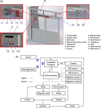
The principle of sliding doors was chosen because it is adapted to the requirements of space-saving and often has a large number of people coming in or leaving. The sliding door is driven by a stepper motor incorporated into a timing belt drive system. This configuration enables the door to change the speed profile when opening and closing. In addition, the timing belt is light and clean, allowing the transmission to be positioned on top to save space and easily clean the ground. An intuitive illustration of the designed system, including the mechanical parts, the arrangement of hardware components, and the layout of electrical elements, is presented in Fig. 1. The user’s 3D face image is collected by a depth camera and is only enabled when the first PIR (passive infrared) sensor detects the person outside. The second PIR sensor detects people inside and also people standing at the door to ensure the safety situation when the door is closed. Push-button 1 enables a new user to request registration to the system. Push-button 2 helps people who are not registered in the system, but request to enter. The switching actions with the PIR sensors 1 and 2 help to ensure the door is always closed and opened at the controlled positions. The magnetic lock is used to maintain the closed state if there is any unauthorized intrusion.
The application design of access control system: (a) The 3D design model and (b) the layout of the electrical components.

The web application helps the administrator to create, edit users, and monitor remote access information. The web application has a user interface displayed in a web browser and communicates with the system hardware using the Hypertext Transfer Protocol. The system will execute the alarm function by notifying the web application in the event of unauthorized access, which is detected by the status of magnetic switches. Specifically, any action that changes the state of the magnetic switch while the recognition system has not been successfully authenticated will be considered unauthorized access and notified to the web application.
3. The 3D Recognition System
3.1. System overview
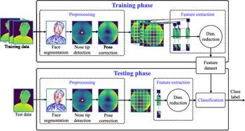
For the application of 3D facial recognition to the access control system, our proposed system consists of the main parts shown in Fig. 2 and briefly described as follows:
-
(i) Since the camera output usually contains other unnecessary information besides face information, a face is detected using simple geometrical features of the head region combined with the Random Sample Consensus (RANSAC) algorithm to separate the fitted head from the data. This part is called face segmentation and is mainly based on related work in [Reference Spreeuwers13].
-
(ii) Because human hairstyle is often changed and sometimes they wear a hat when accessing the system, the face is separated from the fitted head to limit hair occlusion by taking the points located in the sphere, which has the center as the nose tip.
-
(iii) Because face posture can be varied during the recognition process, our proposed system uses the ICP algorithm and RANSAC algorithm to get the parameters of the ICS [Reference Spreeuwers13] for the pose correction purposes.
-
(iv) At the feature extraction stage, the PCA-LDA-based method is used to create a subspace of lower dimension from the training data. When projecting data from each human face to that subspace, the obtained lower-dimensional feature vector can represent the face information with the advantage of efficient computability and storage capacity.
-
(v) Finally, the k-Nearest Neighbors (kNN) algorithm is used to classify feature vectors at the classification stage. The result of this stage is the label or identity of the test data.
Block diagram of the proposed 3D face recognition system.

3.2. Face segmentation
At this stage, the data are first removed from depth points beyond
 $[300\,{\rm mm}; 1000\,{\rm mm}]$
to reduce redundant background information. Following this, the obtained data are downsampled by finding the nearest center point of each voxel with the size of
 $10 \times 10 \times 10\,{\rm mm}$
, which can be illustrated in Fig. 3. This process is mainly used to reduce the computation cost in the face fitting algorithm. The normal of each point is then estimated by using the Open3d library because of their efficiency and speed.
The illustration of down sampling process.

Constructing the cylinder piece by two points and its normal.

Next, the RANSAC algorithm [Reference Fischler and Bolles17] is used to find 3D facial points in the data. RANSAC is an iterative technique that constructs the mathematical model by using the minimal random set of data points. The final result is the model, which has the highest number of inliers in total iterations. The inliers are the points on the facial surface that are modeled reasonably by a cylinder piece and entirely described by Spreeuwers et al. [Reference Spreeuwers13]. The outliers are other body parts like the neck, shoulder, check, and sensor noise like the spike. As stated in references [Reference Spreeuwers13], the RANSAC algorithm has the advantages of its speed and its robustness against outliers.
The cylinder piece is defined by two randomly selected points
 $p_1$
and
 $p_2$
that satisfy the following conditions: the distance between two points in the x-direction
 $dc_x$
is in the range
 $[dc_{x}^{min}, dc_{x}^{max}]$
, and the distance between two points in the y-direction
 $dc_y$
less than
 $dc_{y}^{max}$
. The model parameters are described in Fig. 4. In this Fig. 4,
 $n_1$
and
 $n_2$
are normals of
 $p_1$
and
 $p_2$
respectively, the direction a of the axis of the cylinder is perpendicular to bolt
 $n_1$
and
 $n_2$
,
 $\alpha$
is the plane passing through
 $p_1$
and take
 $b=a \times n_1$
as the normal, l is the line passing through
 $p_2$
and takes
 $n_2$
as the direction,
 $H_2$
is the intersection point of the line l and the plane
 $\alpha$
, the axis of the cylinder is the line passing through
 $H_2$
and the takes a as the direction,
 $H_1$
is the intersection point of the cylinder axis and the line through
 $p_1$
and take
 $n_1$
as the direction vector, C is the center of the cylinder, which is the midpoints of
 $H_1 H_2$
, r and h are the cylinder radius and cylinder height respectively. The consensus
 $C_{cyl}$
is the total number of points, which are satisfied the conditions described as follows:
 \begin{equation} C_{cyl} = \sum_{k} \begin{cases} 1 & \text{if $d(k) \leq d^{max}$ and $d_h(k) \leq h/2$}.\\ 0 & \text{otherwise}. \end{cases}\end{equation}
where
 $C_{cyl}$
is the number of inliers, d(k) is the distance of point
 $p_k$
to the cylinder piece, and
 $d_{h}(k)$
is the distance between the point
 $p_k$
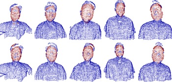
and the center C in the direction of the cylinder axis. The model parameters and the settings used in the RANSAC algorithm are summarized in Table I. The choice of parameters is mainly based on the work of [Reference Spreeuwers13] and our experimental results. Some of examples of the fitted head are shown in Fig. 5.
The model parameters and the settings used in the RANSAC algorithm

Examples of the fitted head (red region), each column shows the results of one person.

The 3D facial point results obtained from RANSAC usually carry redundant information, such as hair and part of the neck, or lose the necessary information due to the incomplete fitting process. Therefore, it is necessary to define a new point as the origin to separate the face region. The tip of the nose is frequently used and is the preliminary step in many 3D facial recognition tasks because of its ease of identification and less affected by facial expression. In our application, face detection is usually done under near frontal poses. Hence, a heuristic estimate of the closest point to the viewer is sufficient in our case. First, the data obtained after RANSAC are rotated around the x-axis (the coordinate system defined in Fig. 7) with the angles
 $\gamma$
in a range of
 $[-\pi/3, \pi/3]$
and a step size of
 $\pi/15$
. For each rotation angle
 $\gamma$
, the closest point to the viewer is calculated and saved as the nose tip candidate. The nose tip candidate with the most occurrences is then used to center a sphere of radius
 $r_n$
(here:
 $80\,{\rm mm}$
). Which nose tip candidate has the highest number of points in the sphere of radius
 $r_n$
is considered as the final nose tip.
An example of nose missing region in fitted head (red points).

The overall process of determining the tip of the nose.

The illustration of Intrinsic Coordinate System parameters.

The RANSAC algorithm worked very well in fitting a head region and did not fail in any case in our experiments. However, the RANSAC algorithm is based on the random sampling technique, so it can sometimes get stuck in models that do not fit the head completely, which leads to the fitted head missing critical areas such as the nose region (see Fig. 6). To solve this problem, we use a fully covered head region window to crop the data from the corresponding range image. Therefore, the nose region is guaranteed to be in the cropped data. This process is illustrated in Fig. 7 below.
3.3. Pose correction
Because our feature extraction method is sensitive to pose variations, so in the next stage, we employ an automatic pose correction algorithm which is mainly based on the novel called ICS. This method is also considered as in [Reference Spreeuwers13]. The ICS is determined by the facial landmarks of the point cloud without having to map one-point cloud to another. In our case, the vertical symmetrical plane of the face and the slope of the nose bridge is used to extract the parameters of the ICS. These parameters contain three angles
 $\phi, \psi, \theta$
and have the origin locate in the nose tip position. The illustration of the ICS is shown in Fig. 8. In that,
 $\alpha$
is the symmetry plane of the face.
 $\phi, \psi$
are the angles formed by
 $\alpha$
with z-axis and y-axis, respectively. The nose bridge, which is fitted with a line
 $d_n$
, is formed with an y-axis angle
 $\theta$
. To get the face pose to the frontal position, the angles
 $\phi$
and
 $\psi$
need to be set to 0 rad and
 $\theta$
to
 $\pi/6$
(according to [Reference Spreeuwers13]).
Next, the ICP [Reference Arun, Huang and Blostein18] algorithm is used to find the symmetry plane parameters that are
 $\phi$
and
 $\psi$
. ICP is an iterative method that finds the Least-Squares solution of the rotation matrix R and the translation vector T so that two point sets
 $P_1=\{p_{1i}\}$
and
 $P_2=\{p_{2i}\}$
can be related by
 \begin{equation} P_2 = R P_1 + T + N\end{equation}
where R is
 $3\,\times\,3$
rotation matrix, T is a translation vector (
 $3 \times 1$
column matrix), and N is a noise vector (
 $3\,\times\,1$
column matrix). First, we define symmetrical face region
 $P_1$
by clipping all points whose distance to the tip of the nose is less than
 $80\,{\rm mm}$
. Next, this region is mirrored in the yz-plane to obtain the point set
 $P_2$
. Our hypothesis is that the half of the rotation angles that transforms
 $P_1$
into
 $P_2$
are the parameters of the symmetry plane of the face region. The algorithm details are implemented in accordance with the following steps:
Step 1: For each point
 $p_{2i}$
in
 $P_2$
, determine the corresponding point
 $p'_{\!\!1i}$
in
 $P_1$
, which has the closest Euclidean distance to
 $p_{2i}$
. The corresponding points form a new point set
 $P'_{\!\!1}$
. Note that,
 $P_2$
and
 $P'_{\!\!1}$
must have the same number of N data points.
Step 2: Respectively calculate the centroids
 $c'_{\!\!1}$
and
 $c_2$
of
 $P'_{\!\!1}$
and
 $P_2$
:
 \begin{equation} c'_{\!\!1}=\dfrac{1}{n}\sum_{i=1}^{n} p'_{\!\!1i} \end{equation}
 \begin{equation} c_2=\dfrac{1}{n}\sum_{i=1}^{n} p_{2i} \end{equation}
Step 3: Subtract each point set for its centroid, we have
 \begin{equation} Q'_{\!\!1} = \lbrace q'_{\!\!1i} \rbrace = \lbrace p'_{\!\!1i} - c'_{\!\!1} \rbrace \end{equation}
 \begin{equation} Q'_{\!\!2} = \lbrace q'_{\!\!2i} \rbrace = \lbrace p'_{\!\!2i} - c'_{\!\!2} \rbrace \end{equation}
Step 4: Calculate the
 $3 \times 3$
matrix:
 \begin{equation} H = \sum_{i=1}^{N} q_{1i} q_{2i}^T\end{equation}
Step 5: Find the SVD of H:
 \begin{equation} USV^T = SVD(H)\end{equation}
Step 6: Calculate
 \begin{equation} R = VU^T \end{equation}
 \begin{equation} T = c_2 - Rc'_{\!\!1} \end{equation}
Step 7: The transformation of
 $P_1$
is calculated by
 \begin{equation} P_1 = R P_1 + T\end{equation}
Step 8: If the convergence condition is not satisfied, go back to Step 1.
As pointed out by Arun, K. Somani et al. [Reference Arun, Huang and Blostein18], the solution of R and T can minimize the least-squares function as follows:
 \begin{equation} \Sigma^2 = \sum_{i=1}^{N} \Vert p_{2i}- (R p_{1i} + T) \Vert^2\end{equation}
Our convergence conditions include the deviation of the mean squared error between two iterations is less than
 $\delta_{max}$
(here:
 $0.01$
) or the number of iterations is less than
 $i_{max}$
(here: 20). Larger
 $\delta_{max}$
and smaller
 $i_{max}$
can improve the accuracy of the algorithm, but choosing such parameters can be very time consuming because of the high computational cost of ICP.
The result of the rotation matrix R has the form of:
 \begin{equation} R = R_z(\alpha) R_y(\beta) R_x(\gamma)\end{equation}
where
 $R_z(\alpha), R_y(\beta), R_x(\gamma)$
are the rotation matrices about z-axis, y-axis, and x-axis, respectively. Because
 $P_2$
is a mirror of
 $P_1$
through the yz-plane,
 $\gamma$
has a value of 0 rad in our case. Thus, the rotation matrix R can be written as
 \begin{equation} R = \begin{bmatrix} cos(\alpha)cos(\beta)\;\;\;\;\; & -sin(\alpha)\;\;\;\;\; & cos(\alpha)sin(\beta)\\ sin(\alpha)cos(\beta)\;\;\;\;\; & cos(\alpha)\;\;\;\;\; & sin(\alpha)sin(\beta)\\ -sin(\beta)\;\;\;\;\; & 0\;\;\;\;\; & cos(\beta) \end{bmatrix}\end{equation}
Therefore, the symmetry plane parameters can be calculated as
 \begin{equation} \phi = -\dfrac{\alpha}{2} = -\dfrac{1}{2} atan2 \left(-\dfrac{R_{12}}{R_{22}}\right) \end{equation}
 \begin{equation} \psi = -\dfrac{\beta}{2} = -\dfrac{1}{2} atan2\left(-\dfrac{R_{31}}{R_{33}}\right) \end{equation}
The final parameter of the ICS, which is the nose bridge angle
 $\theta$
, is determined by fitting a line to the facial data above the nose tip. First, the pose of the facial point is corrected by rotating the data so that the
 $\phi$
and
 $\psi$
angles are set to 0 rad. Then, the facial region above the nose tip is extracted by a half sphere with a radius of
 $35\,{\rm mm}$
. Then, the extracted facial region is projected onto the yz-plane to take the 2D nose bridge profile (see Fig. 9). Since the nose bridge is the longest straight line in a 2D nose bridge profile, we use the RANSAC algorithm to estimate the nose bridge line parameters. The combination of two points is used to construct the straight-line model, the first one is the near nose tip point (distance from the nose tip is less than
 $10\,{\rm mm}$
), and the second one is the randomly selected point of the rest data. The consensus of a line is calculated by counting the points which satisfy the conditions as follows:
 \begin{equation} C_{l} = \sum_{k} \begin{cases} 1 & \text{if $d_{l}(k) \leq 3\,{\rm mm}$}.\\ 0 & \text{otherwise}. \end{cases}\end{equation}
where
 $C_l$
is the number of inliers in nose bridge model and
 $d_l(k)$
is the distance from the point k to the line. The model with the highest inliers is chosen as the best fit. Note that this algorithm is implemented in the 2D nose bridge profile points. Therefore, this approach is more accurate and takes less time-consuming than 3D face data.
(a) Illustration of the region above the nose tip. (b) The 2D nose bridge profile in yz-plane.

The angle
 $\gamma$
defining the tilt angle of the head, the facial data are rotated so that the
 $\gamma$
is equal to
 $\pi/6$
, resulting in the face being brought back to the frontal view.
The final step in this phase is the separation of the region of interest. First, the entirely corrected facial data is converted into a range image. Then, a Median filter is applied for filling holes caused by the pose correction. The tip of the nose is then again determined by finding the point which has a minimum z value. Finally, we cut out the elliptical region with a horizontal radius of
 $60\,{\rm mm}$
and the vertical radius of
 $70\,{\rm mm},$
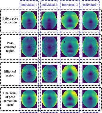
centered at the nose tip. Selecting the large radius results in more face information are obtained. However, it also includes undesired areas such as the background, neck, ears, or hair. Figure 10 shows some examples of pose correction results.
Examples of pose correction results.

3.4. Feature extraction
In this stage, we use the feature extraction method based on the combination of principal component analysis (PCA) and linear discriminant analysis (LDA), which is known as Fisherface [Reference Belhumeur, Hespanha, Kriegman and Anal19] in 2D face recognition. The main idea of this method is that the most important information contained in the face image can be extracted by PCA and use LDA to transform the obtained information into the data more reliable for classification. PCA is a method that finds a projection matrix
 $U_k$
that can keep the most information from the original data in the k dimensions. The method of finding
 $U_k$
is described as below.
Each facial image resulting from the pose correction stage is reshaped into a column vector
 $x_i$
. Therefore, for n the people in the training data set, we have a large column matrix X with n column
 $x_i$
. The average face
 $\bar{x}$
is given by
 \begin{equation} \bar{x} = \dfrac{1}{n} \sum_{i=1}^{n} {x_i}\end{equation}
Each face
 $x_i$
differs from the average
 $\bar{x}$
by the vector
 $\hat{x}_i$
:
 \begin{equation} \hat{x}_i = x_i - \bar{x}\end{equation}
The mean subtracted data
 $\hat{X}$
is defined by a set of n column vector
 $\hat{x}_i$
. The covariance matrix C of
 $\hat{X}$
is given by
 \begin{equation} C = \dfrac{1}{n-1} \hat{X} \hat{X}^T\end{equation}
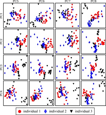
A 2D projection of the first eight principal components of three individuals.

The principal components are then obtained by calculating the Eigen-Decomposition of C and sorting them in descending order of the eigenvalues. The first k eigenvectors form a new subspace
 $U_k$
. When projecting
 $\hat{X}$
to this subspace, the obtained new data can be calculated as follows:
 \begin{equation} Z = U_{k}^{T} \hat{X} \end{equation}
The initial data can be approximated by
 \begin{equation} \tilde{X} = U_{k} Z + \bar{x} \end{equation}
Equations (17) and (18) show that Z (size
 $k \times n$
) can describe the original face data with only k dimensions. Therefore, it is possible to create an efficient classification algorithm that can classify individuals through the feature vectors
 $z_i$
which is obtained from Z. In Fig. 11, we extracted the first eight principal components of three individuals and plotted them in 2D space. The result shows that the features of these individuals are not separate (such as
 $PC1-PC5, PC2-PC7,...$
), and therefore, it is complicated to build a classification model for this data. We use linear discriminant analysis (LDA) to find the optimal projection that can transform Z into more reliable data for classification. The projection matrix W is selected in such a way that:
 \begin{equation} W = \underset{W}{\mathrm{argmax}} \dfrac{\vert W^T S_B W \vert} {\vert W^T S_W W \vert}\end{equation}
where
 $S_W$
and
 $S_B$
are the between-class scatter matrix and within-class scatter matrix, respectively.
 $S_W$
and
 $S_B$
are given by
 \begin{equation} S_W = \sum_{c=1}^{C} \sum_{z \in Z_c} {(z_i - \mu_c)(z_i - \mu_c)^T} \end{equation}
 \begin{equation} S_B = \sum_{c=1}^{C} {N_c(\mu_c-\mu)(\mu_c-\mu)^T} \end{equation}
where
 $\lbrace z_i \vert i = 1,2,...,N_c \rbrace$
is the set of feature vectors in class
 $Z_c$
;
 $N_c$
is the number of samples in class
 $Z_c$
; C is the number of classes;
 $\mu_c$
and
 $\mu$
are the mean feature vector of class
 $Z_c$
and Z, respectively. The
 $\mu_c$
and
 $\mu$
are calculated as follows:
 \begin{equation} \mu_c = \dfrac{1}{N_c} \sum_{i=1}^{N_c} {z_i} \end{equation}
 \begin{equation} \mu = \dfrac{1}{n} \sum_{i=1}^{n} {z_i} \end{equation}
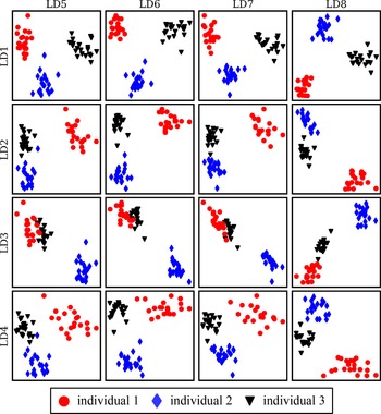
The 2D projection of the first eight components of three individuals extracted by the LDA method

If
 $S_W$
is nonsingular, the projection matrix W is the set of eigenvectors
 $\lbrace w_i \vert i = 1,2,...,C-1 \rbrace$
of
 $S_W$
and
 $S_B$
corresponding to the largest eigenvalues
 $\lbrace \lambda_i \vert i = 1,2,...,C-1 \rbrace$
:
 \begin{equation} S_{W}^{-1} S_B W = W \lambda\end{equation}
The final set of feature vectors in this stage is given by
 \begin{equation} F = W^T Z\end{equation}
In Fig. 12, we extracted the first eight components of the LDA method to illustrate the benefits of the PCA-LDA-based feature extraction. Compared to the previous PCA method (see Fig. 11), the new feature vectors are now clearly separated. As a result, we can construct a much more simplistic and efficient classifier based on these data.
3.5. Features classification
In this step, we use k-Nearest Neighbor (kNN) algorithm to determine the identity of the new input feature vector
 $f_{new}$
by the data set F obtained from the training stage. First, all rows of F and
 $f_{new}$
are normalized in the range between 0 and 1. Next, we calculate the Euclidean distances
 $d_i$
between
 $f_{new}$
and feature vector
 $f_i$
. After that, each
 $f_i$
in the first k nearest neighbors is chosen and assigned a weight
 $w_i$
(i=1,2,…,k) so that
 $w_i$
decreases as
 $d_i$
increases. Our expression of W as follows:
 \begin{equation} w_i = e^{-\dfrac{d_{i}^{2}}{\sigma^2}}\end{equation}
where the weight
 $w_i$
is close to 1 when the distances
 $d_i$
is close to 0;
 $\sigma$
is a positive number and affects the change of
 $w_i$
by the change of
 $d_i$
. To determine the identity of the input feature vector, we use the label of the person who has the highest match score in k nearest neighbors. The matching score is calculated as follows:
 \begin{equation} s_m = \sum^{j}_{i=1}{w_i}\end{equation}
where:
 $s_m$
is the matching score of person m; j is the number of occurrences of person m in k nearest neighbors. This parameter may also serve as the threshold for verification tasks. In detail, when a person has a matching score
 $s_m$
larger than a threshold
 $\theta_{VR}$
, this person is accepted by the system.
3.6. Experimental results
3.6.1 The description of data set
First, 3D data of Biomech Lab (HCMUT Viet Nam) members were collected to assess the performance of the algorithm. Due to the equipment limitations, our experiment uses a low-cost depth sensor, Intel RealSense D415, to capture images in the range between
 $0.3$
and
 $1.0$
m and with a sampling time of 1s.
The reason why the operating distance of the camera was chosen to be between
 $0.3$
and
 $1.0$
m is the limitation of the camera accuracy. The manufacture’s catalog indicates that, at distances greater than 2 m, camera errors may reach 2%. However, based on the experimental results in [Reference Carfagni, Furferi, Governi, Santarelli, Servi, Uccheddu and Volpe20], the highest reconstruction error is approximately
 $0.081$
to
 $2.571\,{\rm mm}$
at a distance of
 $0.3$
to
 $1.0$
m, which is more suitable for our face recognition application. With this operating range limitation, our system requires the user to stand still in front of the camera to carry out sampling and recognition. However, with the configuration: 90 fps at
 $640 \times 480$
resolution, the Intel RealSense D415 can capture the images without motion blur or depth artifacts (caused by the camera using rolling shutter technology), even in cases where the user moves their face quite fast, around
 $1.7$
to 2 m/s.
The images were captured under illuminance of 400 Lux, which is suitable for office and laboratory environments. However, based on the experimental results in the white paper Projector for Intel RealSense Depth Cameras D4xx provided by Intel, the D415 model can work well in environments with an ambient light condition of approximately 25 Lux. This mean that even in low-light conditions, the proposed system can still operate as intended.
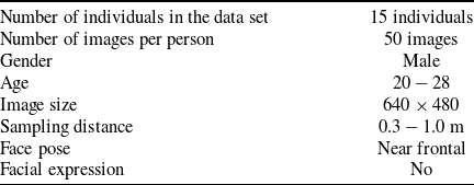
In total, the data set contains 750 range images of 15 person with detailed information shown in Table II. The purpose of this experiment is to verify the precision, accuracy, and also the feasibility of our proposed algorithm.
The details of our 3D facial data set

The plot of rank-1 IR versus the variation of the number of samples per person.

The plot of rank-1 IR versus the variation of the number of principal components.

3.6.2 The parameters selection
To assess the performance of our recognition system, the cumulative match curve (CMC) and the receiver operating characteristic curve (ROC curve) are used. The CMC measures the performance of identification system by plotting the identification rate (IR) relative to the rank distribution. IR is the probability that the identity of probes is correctly recognized while the rank distribution shows the ranked matching rate when a probe is compared to all faces in the data set. Depending on the security requirements of the application, the results of each rank can be used. The lower the rank used, the higher the security of the system. The ROC curve measures the performance of the verification system by plotting the verification rate (VR) relative to the false acceptance rate (FAR). The VR is the probability that genuine probes are accepted by the system, while the FAR is the probability that fake probes are accepted by the system.
The plot of rank-1 IR versus the variation of LDA dimensions.

The plot of rank-1 IR versus the variation of
 $\sigma$
value

Our system has the following important parameters that need to be specified: the number of samples per person in the training data set, the number of components of the PCA-LDA method at feature extraction stage, and the
 $\sigma$
value of the weighted function at the classification stage. To determine each parameter independently, we changed the parameters to be determined and fixed the remaining parameters to evaluate the change of the performance criterion, which is the rank-1 identification rate (rank-1 IR).
As seen in Fig. 13, which shows the plot of rank-1 identification rate versus the variation of the number of samples per person in the training data set, the system archives the lowest rank-1 IR for the training data set with at most of two samples per person. By increasing the number of samples, the recognition rate also increases and remains nearly unchanged after four samples per person. However, if only a small number of samples are selected, the system performance can be degraded in actual operations due to failed sampling or preprocessing. On the other hand, choosing too many samples also increases the computational cost, training time, and storage capacity of the system. We have selected 10 training samples per person to compromise these performances.
The maximum number of principal components depends on the size of the training data set and should not be greater than the total number of samples. In this experiment, we used 10 images per person to create the training data set. The number of components was changed from 10 to 140, while the other parameters were fixed. It can be observed in Fig. 14, the rank-1 IR remains nearly unchanged when the number of dimension changes from 20 to 100 and starts to decrease sharply from 120 onwards. While the accuracy results were not significantly different, we only selected the first 20 principal components due to their advantage in terms of storage and computational.
Figure 15 shows a plot of rank-1 IR with the number of LDA dimensions varying from 1 to 14, which is the number of individuals in the training data set minus one. The remaining parameters are fixed, such as the number of principal components is 20 and the value of
 $\sigma$
is
 $0.1$
. It can be observed that the accuracy increases as the number of LDA dimensions increases. Therefore, the rank-1 IR reaches its maximum value when the number of LDA dimensions is 14.
The final parameter that needs to be determined is the
 $\sigma$
value of the weighted function at the classification stage. In this experiment, the
 $\sigma$
value was changed from 0 to 1, while the number of principal components and the numbers of LDA dimensions were fixed at 20 and 14, respectively. In Fig. 16, which shown the plot of rank-1 IR versus the variation of
 $\sigma$
value, the system accuracy remained nearly unchanged when the
 $\sigma$
value reached
 $0.02$
or higher.
3.6.3 Evaluate the system performance
(a) Computational performance and storage capability
We summarize the results of the execution time of each stage in the proposed 3D face recognition system in Table III. All results were implemented in the Python language and tested on a computer equipped with Intel Core i5-8300H 2.30GHz processor and 8GB RAM. The results show that the total recognition time (sum of face segmentation, pose correction, and classification time) for each person is about
 $1.388+1.517+0.271/150=2.905$
s, in that the preprocessing stage takes most of the recognition time (almost
 $2.905s$
in total). The feature extraction time is neglected since this stage carries out only one matrix multiplication at the test phase.
The identification time of each stage in the proposed 3D face recognition system

With the selected parameters of the PCA-LDA method, it can be concluded that the human face with a complex 3D structure obtained from the depth camera can be represented as a vector with a size equal to the number of dimensions of the LDA. In detail, each original image with size
 $640 \times 480$
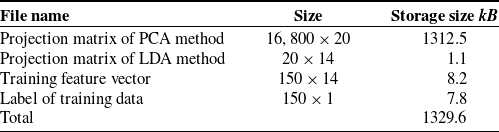
(around 750 kB) can be compressed into a vector with only 14 floating-point numbers, which is approximately 56 bytes. Table IV summarizes the files and their storage size of our data set after the training phase in the proposed approach.
(b) Accuracy performance
Figures 17 and 18 show the plot of the CMC and ROC curve of the system with selected parameters, respectively. The results show that the recognition system that is tested on our data set to achieve a rank-1 identification rate of 98% and a verification rate of 88% at
 $0.1\%$
FAR.
The storage size of files in proposed approach

The CMC plot of the proposed 3D face recognition system

The ROC curve of the proposed 3D face recognition system

4. Conclusion and Future Works
In this work, we proposed the 3D face recognition algorithm for application in the access control system. By using the proposed algorithm, the access control system may both inherit the advantages and overcome some disadvantages of the traditional 2D face recognition methods. The system is capable of cropping human face in 3D data and recognizing the face in near frontal positions with an accuracy of 98% at rank-1 identification rate and verification rate of 88% at
 $0.1\% $
FAR. In addition, by using the PCA algorithm in combination with LDA, the characteristics of individuals are better separated and more effective in storage. The experimental times show that the proposed algorithm is relatively fast at the feature extraction and classification stages (1.8 ms for each data sample), but the preprocessing stage is slow, especially in the pose correction because of the ICP algorithm. The nose tip detection algorithm is sensitive to changes in pose, especially for the z-axis. The system parameters are chosen primarily from experiments and related work, but are not optimized. However, the proposed method proved to be quite good in accuracy and precision, feasible, and does not require much expensive equipment for the entire access control system.
In actual operation, the proposed system is not yet suitable for real-time applications due to the slow recognition time of each sample. The operating distance limitation of the 3D camera makes the system incapable of recognizing people from a long distance, so the user is required to stand still in front of the camera during the recognition process. As a result, this limitation makes the proposed system difficult to adapt to large-area activity control and behavior prediction applications independently. However, as the system is designed as a module, it can be easily expanded and installed in many places in buildings where higher security is required, including in workplaces, laboratories, schools, and hospitals. In addition to securing an area, the proposed algorithm may also be applied in systems to check and limit access to machinery and equipment. Furthermore, it also helps improve user and robot interoperability by identifying people. Therefore, the robots can provide separate services to each person. This capability is very important in service robot applications, which should work in many fields with many different lighting conditions.
Future work will focus on improving the stability and accuracy of the nose tip detection algorithm. The recognition speed and accuracy can be improved through optimization of parameters by evolutionary algorithms (such as Genetic Algorithm and Particle Swarm Optimization).
Conflicts of Interest
The authors declare that there is no conflict of interests.
Financial Support
None.
Ethical Considerations
None.
Authors’ Contributions
Mr. Tuong Quan Vo is the principal author and the corresponding author. He is in charge of the main ideas to build up this research topic. He is also responsible for the sketch design of the mechanical, electrical – electronics, and the solution of image processing for this research topic. He also corrects the technologies and engineering issues of this article. Mr. Quoc Dien Le is also the principal author who writes the first draft of this article and proposes solutions about using the 3D face recognition method to solve the Access Control System. Besides, Mr. Quoc Dien Le also contributes to the data collection and training method to operate this system. Mr. Tran Thanh Cong Vu contributes to the ideas of the experimental setup and also the data processing to this research topic. All the authors have read and agreed to the published version of this manuscript.