




1 Introduction
In recent years, much has been uncovered about the nature of the turbulent boundary layer over rough walls. However, compared to the less-practical hydrodynamically smooth flow, there are still outstanding questions. The prevailing theory on the rough-wall turbulent boundary layer pressure spectrum ( $\unicode[STIX]{x1D6F7}(\unicode[STIX]{x1D714})$, where
 $\unicode[STIX]{x1D714}$ is frequency) is a two-layer model: a slow-rising (
 $\unicode[STIX]{x1D714}^{2}$) low-frequency region and a rapidly decaying (
 $\unicode[STIX]{x1D714}^{-5}$) high-frequency region (Blake Reference Blake and Blake2017). These two regions then overlap in the slowly decaying (
 $\unicode[STIX]{x1D714}^{-1}$) mid-frequency. This two-layer model, its expected spectral slopes and the idea of an ‘overlap’ region, have been adopted from rigorous investigations into the smooth-wall-pressure spectrum (Blake Reference Blake1970, Reference Blake and Blake2017; Panton & Linebarger Reference Panton and Linebarger1974; Panton et al. Reference Panton, Goldman, Lowery and Reischman1980; McGrath & Simpson Reference McGrath and Simpson1987; Choi & Moin Reference Choi and Moin1990; Farabee & Casarella Reference Farabee and Casarella1991; Gravante et al. Reference Gravante, Naguib, Wark and Nagib1998; Goody & Simpson Reference Goody and Simpson1999; Smol’yakov Reference Smol’yakov2000; Goody Reference Goody2004). Extending this model to rough-wall flows is considered appropriate because of wall similarity and its associated scale separation. This concept suggests that, if there is a large enough separation between the scales of the largest turbulent eddies and the roughness length scales, the outer-layer flow will be independent of the wall conditions. Sufficient scale separation occurs when the roughness is small compared to the boundary layer height,
 $\unicode[STIX]{x1D6FF}$. The accepted criterion is
 $\unicode[STIX]{x1D6FF}/k_{g}>40$ (Jimenez Reference Jimenez2004), where
 $k_{g}$ is the geometric roughness element height. The Reynolds number must also be high,
 $Re_{\unicode[STIX]{x1D703}}>$ 50 000, where
 $\unicode[STIX]{x1D703}$ is the momentum thickness. At such conditions the influence of roughness on the logarithmic layer is suggested to be vastly diminished. Proof of scale separation was indirectly given by Meyers, Forest & Devenport (Reference Meyers, Forest and Devenport2015) who were able to reveal a previously undetected scaling region within the pressure spectrum, because of their large
 $\unicode[STIX]{x1D6FF}/k_{g}$ and
 $Re_{\unicode[STIX]{x1D703}}$. Wall similarity itself is a compelling argument, supported by several researchers (Raupach, Antonia & Rajagopalan Reference Raupach, Antonia and Rajagopalan1991; Flack, Schultz & Shapiro Reference Flack, Schultz and Shapiro2005; Schultz & Flack Reference Schultz and Flack2007, Reference Schultz and Flack2009), because it implies that the outer flow scaling is truly universal at practical conditions. Flack et al. (Reference Flack, Schultz and Shapiro2005), using sandpaper and woven mesh rough surfaces to simulate fouled blades and tubes, found that the differences in rough-wall boundary layers are confined to
 $y<5k_{s}$ (where
 $k_{s}$ is the equivalent sand grain roughness) in their mean velocity profiles, Reynolds stresses and velocity triple products. These experiments were carried out at
 $Re_{\unicode[STIX]{x1D703}}\approx 14\,000$ and
 $\unicode[STIX]{x1D6FF}/k_{s}\geqslant 40$. They went on to suggest that
 $\unicode[STIX]{x1D6FF}/k_{s}$ is a more appropriate reference for gauging wall similarity than
 $\unicode[STIX]{x1D6FF}/k_{g}$. Nevertheless, there is evidence that the wall-similarity concept needs further review (Krogstad, Antonia & Browne Reference Krogstad, Antonia and Browne1992; Bhaganagara, Coleman & Kim Reference Bhaganagara, Coleman and Kim2007). The premise that smooth- and rough-wall boundary layers share a general form inherently assumes that the interstitial flow and turbulent structures produced by the roughness elements are accounted for in the smooth-wall model. This, even at very high Reynolds numbers, may be an erroneous assumption. Krogstad et al. (Reference Krogstad, Antonia and Browne1992) found that smooth- and rough-wall turbulent boundary layers show deviations over a significant portion of the layer, not just within the near-wall region. Most recently, the experiments of Joseph (Reference Joseph2017) did not show proof of wall similarity, despite exceeding both qualifying criteria.
Another generally accepted concept is that all wall-bounded rough-wall flows fall into one of three categories: hydrodynamically smooth, transitionally rough and fully rough. These categories arise from the early pipe flow studies of Nikuradse (Reference Nikuradse1950), which proposed that the roughness Reynolds number,  $k_{g}^{+}=k_{g}U_{\unicode[STIX]{x1D70F}}/\unicode[STIX]{x1D708}$ (where
 $U_{\unicode[STIX]{x1D70F}}$ is the friction velocity and
 $\unicode[STIX]{x1D708}$ is kinematic viscosity), specifies the extent to which the roughness disrupts the mean flow. Fully rough flows have
 $k_{g}^{+}\geqslant 40$ (Ligrani & Moffat Reference Ligrani and Moffat1986; Jimenez Reference Jimenez2004) and are of most practical interest because it is believed that viscous effects are negligible in this regime and the roughness elements project into the log layer. However, some recent works (Mehdi, Klewicki & White Reference Mehdi, Klewicki and White2013; Meyers et al. Reference Meyers, Forest and Devenport2015) have challenged the community to re-think these assumptions about the extent of viscous effects at high Reynolds numbers.
These concepts, along with established turbulent boundary layer theory, form the basis for existing rough-wall-pressure spectrum scalings. While smooth-wall scalings have been developed somewhat satisfactorily, even yielding promising empirical functions to predict such spectra (Goody Reference Goody2004), there has been relatively less success in scaling rough-wall flows. The recent study of Meyers et al. (Reference Meyers, Forest and Devenport2015) achieved exceptionally high Reynolds numbers and sufficiently large scale separation, allowing them to see that the two-layer/overlap spectral model is a simplification of the actual mid-frequency physics. They tested three rough surfaces along with a smooth-wall ‘baseline’ surface. The rough surfaces consisted of ordered and quasi-randomly distributed hemispheres, and two roughness heights. Because all three rough surfaces consisted of the same element shape and roughness element-to-element spacing, they were able to isolate the effect of  $k_{g}$ and roughness element distribution on the pressure spectra. Element-to-element spacing is typically characterised by the sparseness ratio,
 $\unicode[STIX]{x1D706}$, which is the ratio of the forward projected area of the elements (
 $A_{f}$) to their planform area (
 $A_{w}$). Therefore small
 $\unicode[STIX]{x1D706}$ corresponds to widely separated elements and large
 $\unicode[STIX]{x1D706}$ represents closer element spacing. All the hemispheres of Meyers et al. had
 $\unicode[STIX]{x1D706}=0.052$. The resulting flows had
 $k_{g}^{+}$ ranging from 91 to 507 and
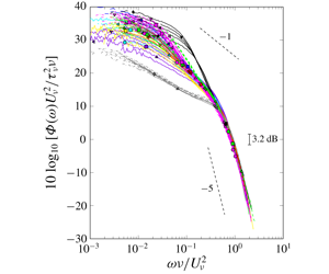
 $\unicode[STIX]{x1D6FF}/k_{g}$ from 72 to 212, such that all cases were in the fully rough flow regime. A distinctive mid-frequency region was uncovered because of the large separation between roughness scales and the viscous scales. Meyers et al. thus proposed the triple scaling hypothesis, which states that the rough-wall-pressure spectrum comprises of three independent scaling regions, as opposed to two regions and an overlap region. They hypothesised that the mid-frequency region comprises of the roughness scales and so the previously proposed high-frequency scalings are actually mid-frequency scalings. Correspondingly, the high-frequency region is governed purely by viscosity and is independent of the roughness scale, behaving much like the high-frequency region of the smooth-wall boundary layer. This new understanding led to a proposed universal high-frequency scaling law of
 $\unicode[STIX]{x1D6F7}(\unicode[STIX]{x1D714})U_{\unicode[STIX]{x1D708}}/(\unicode[STIX]{x1D70F}_{\unicode[STIX]{x1D708}}^{2}\unicode[STIX]{x1D708})$ versus
 $\unicode[STIX]{x1D714}\unicode[STIX]{x1D708}/U_{\unicode[STIX]{x1D708}}^{2}$;
 $U_{\unicode[STIX]{x1D708}}$ in this scaling was referred to as the shear friction velocity and was interpreted as the portion of
 $U_{\unicode[STIX]{x1D70F}}$ which does not include the pressure drag on the roughness elements;
 $\unicode[STIX]{x1D70F}_{\unicode[STIX]{x1D708}}$ is the corresponding shear stress. Meyers et al. showed that this scaling collapsed the pressure spectra of hemispherical roughness with
 $k_{g}=[3~\text{mm},1~\text{mm}]$; randomly distributed and ordered hemispheres; the sparse 1 mm hemispheres of Varano (Reference Varano2010); the sand grains of Blake (Reference Blake1970) (dense large, dense small, sparse small); and the sand grains of Aupperle & Lambert (Reference Aupperle and Lambert1970) for all
 $\unicode[STIX]{x1D714}\unicode[STIX]{x1D708}/U_{\unicode[STIX]{x1D708}}^{2}\gtrsim 0.6$. However, the
 $U_{\unicode[STIX]{x1D708}}$ scaling has yet to be systematically validated with roughness of different shapes, or surfaces comprising of two or more roughness geometries. Scaling roughness of different element densities also requires a second look because the data sets which varied this parameter (Blake Reference Blake1970; Varano Reference Varano2010) were obtained at relatively low Reynolds numbers.
Summary of pressure spectrum scalings, categorised according to the triple scaling hypothesis.

Meyers et al. also examined the effectiveness of existing rough-wall-pressure spectrum scalings using their high Reynolds number data set, which is particularly useful since theirs is one of the few data sets which meets both criteria for universal scaling laws. A summary of some of these existing scalings is presented in table 1. In the low-frequency region the two most well-known scalings are the classical smooth-wall scaling and the mixed-outer scaling of Blake (Reference Blake1970), both originally developed for scaling the smooth-wall-pressure spectrum, but because of the assumption of wall similarity are extended to rough-wall flows. The classical outer scaling,  $\unicode[STIX]{x1D6F7}(\unicode[STIX]{x1D714})U_{\unicode[STIX]{x1D70F}}/\unicode[STIX]{x1D70F}_{w}^{2}\unicode[STIX]{x1D6FF}$ versus
 $\unicode[STIX]{x1D714}\unicode[STIX]{x1D6FF}/U_{\unicode[STIX]{x1D70F}}$, has successfully collapsed smooth-wall data in numerous studies. It uses the boundary layer thickness,
 $\unicode[STIX]{x1D6FF}$, as a length scaling because the low-frequency eddies are expected to have a size of the order of
 $\unicode[STIX]{x1D6FF}$. The friction velocity,
 $U_{\unicode[STIX]{x1D70F}}$, is the chosen velocity scale because, based on the defect law, it is assumed that the wall shear stress,
 $\unicode[STIX]{x1D70F}_{w}$, controls the velocity gradient in the outer portion of the boundary layer. Blake (Reference Blake1970) modified this scaling by using the displacement height,
 $\unicode[STIX]{x1D6FF}^{\ast }$, as the scaling length and the edge velocity,
 $U_{e}$, as the scaling velocity. He suggested that these were more appropriate parameters because they better reflected the nature of the outer region flow, producing a final scaling of
 $\unicode[STIX]{x1D6F7}(\unicode[STIX]{x1D714})U_{e}/\unicode[STIX]{x1D70F}_{w}^{2}\unicode[STIX]{x1D6FF}^{\ast }$ versus
 $\unicode[STIX]{x1D714}\unicode[STIX]{x1D6FF}^{\ast }/U_{e}$. Meyers et al. (Reference Meyers, Forest and Devenport2015) applied these scalings to their data and the data sets of Blake (Reference Blake1970), Aupperle & Lambert (Reference Aupperle and Lambert1970) and Varano (Reference Varano2010) to show that neither is able to convincingly collapse all of the data, especially at very low frequencies where they should be most effective. Joseph (Reference Joseph2017) later quantified this lack of collapse more definitely through uncertainty analysis.
According to the triple scaling hypothesis, the previously proposed high-frequency scalings, which are based on geometric roughness features, are actually mid-frequency scalings. These mid-frequency scalings were also tested by Meyers et al. and were found to be even less successful than the low-frequency scalings. The empirical inner scaling of Aupperle & Lambert (Reference Aupperle and Lambert1970),  $\unicode[STIX]{x1D6F7}(\unicode[STIX]{x1D714})U_{\unicode[STIX]{x1D70F}}/(\unicode[STIX]{x1D70F}_{w}^{2}k_{s}C_{f})$ versus
 $\unicode[STIX]{x1D714}k_{s}/U_{\unicode[STIX]{x1D70F}}$, showed only marginal success on data sets other than their own sparsely populated, uniformly distributed sand particles. In the latter scaling
 $C_{f}$ is the non-dimensional skin-friction coefficient. Blake (Reference Blake1970) proposed a mid-frequency scaling from his experiments on sparsely packed small roughness, densely packed large roughness and densely packed small roughness:
 $\unicode[STIX]{x1D6F7}(\unicode[STIX]{x1D714})U_{\unicode[STIX]{x1D70F}}/\unicode[STIX]{x1D70F}_{w}^{2}k_{g}$ versus
 $\unicode[STIX]{x1D714}k_{g}/U_{\unicode[STIX]{x1D70F}}$. This is very similar to his proposed low-frequency scaling except that the chosen length scale is
 $k_{g}$ to account for the roughness length scales, and
 $U_{\unicode[STIX]{x1D70F}}$ is the velocity scale because he believed that
 $\unicode[STIX]{x1D70F}_{w}$ is the only external stress on the boundary layer. The resulting scaling is the Strouhal number of the roughness elements. Presently, Blake’s inner scaling is deemed the most successful scaling for the widest range of rough-wall flows (Varano Reference Varano2010; Forest & Devenport Reference Forest and Devenport2011). Varano (Reference Varano2010) later proposed a mid-frequency scaling based on his experiments with sparse, ordered hemispherical roughness at 20 and
 $27~\text{m}~\text{s}^{-1}$. He suggested that
 $U_{\unicode[STIX]{x1D70F}}$ should be proportional to
 $U_{e}$ in the fully rough regime, which allowed him to substitute
 $U_{e}$ into Blake’s inner scaling to produce
 $\unicode[STIX]{x1D6F7}(\unicode[STIX]{x1D714})/\unicode[STIX]{x1D70C}^{2}U_{e}^{3}k_{g}$ versus
 $\unicode[STIX]{x1D714}k_{g}/U_{e}$. This scaling was able to successfully collapse a significant amount of Varano’s data. Meyers et al. also proved that this scaling is at least as successful as Blake’s inner scaling for roughnesses of different
 $k_{g}$, and both ordered and random element distributions. Mixed-inner–outer scalings, such as those of De Graaff & Eaton (Reference De Graaff and Eaton2000), Forest (Reference Forest2012) and Klewicki (Reference Klewicki2013), have also been proposed. These attempt to uncover intermediary scales which characterise statistical properties of the outer flow. This idea is promising as such velocity and length scales would represent the largest scales in the outer flow and also account for the effect of roughness scales on the outer flow. Klewicki (Reference Klewicki2013), for example, explains that his inner–outer-layer intermediate length-scale normalisation for smooth walls,
 $\unicode[STIX]{x1D6FF}\unicode[STIX]{x1D708}/U_{\unicode[STIX]{x1D70F}}$, represents an average property of the underlying layer width distribution. Similarly De Graaff & Eaton (Reference De Graaff and Eaton2000) explored a mixed inner–outer velocity scaling for collapsing the streamwise fluctuating velocity in smooth-wall turbulent boundary layers. Joseph (Reference Joseph2017) explored the effectiveness of these for pressure spectra using hybrid scalings based on these (see table 1) and found that they were less than ideal. It is also prudent to point out that even the most successful of these mid-frequency scalings have not produced the hypothesised
 $-1$ slope which is derived from dimensional analysis of the smooth-wall-pressure spectrum (Blake Reference Blake1970; Panton & Linebarger Reference Panton and Linebarger1974). The expectation of a
 $-1$ mid-frequency slope assumes the characteristics of both the high- and low-frequency regions are shared in an ‘overlap’ mid-frequency region. With the assumption of wall similarity one might expect this
 $-1$ overlap region to also be apparent in rough-wall flows. However, most studies have not produced this mid-frequency slope. In fact, even a number of studies of smooth-wall boundary layers show a constant-slope mid-frequency region with slope between
 $-0.7$ and
 $-0.8$ (Blake Reference Blake1970; McGrath & Simpson Reference McGrath and Simpson1987; Goody & Simpson Reference Goody and Simpson1999). This calls into question the fundamental premise of an overlap region. To date, the
 $-1$ slope has only been observed in simulations (Lee, Blake & Farabee Reference Lee, Blake and Farabee2005) and the experimental work of Klewicki, Priyadarshana & Metzger (Reference Klewicki, Priyadarshana and Metzger2008) on transitionally rough atmospheric boundary layers.
Scaling rough-wall boundary layers of diverse geometries is an important step toward scaling realistic rough-wall flows. However, the specific effect of different geometric parameters on the pressure spectrum is not clear, which complicates the process of scaling the spectrum. Roughness element height is thought to influence the medium and very small-scale turbulent structures (Blake Reference Blake1970). This is supported by Meyers et al. (Reference Meyers, Forest and Devenport2015), who found the slope of the mid-frequency region changes depending on the roughness height. The arrangement of roughness elements (ordered, quasi-random, straight, staggered) is reported as having minimal impact on the pressure spectrum, particularly outside the near-wall region (Waigh & Kind Reference Waigh and Kind1998; George & Simpson Reference George and Simpson2000; Meyers et al. Reference Meyers, Forest and Devenport2015). Roughness element shape is probably the most widely researched geometric roughness parameter. Common shapes are hemispheres (Tomkins Reference Tomkins2001; Bennington Reference Bennington2004; Hopkins Reference Hopkins2010; Varano Reference Varano2010; Forest & Devenport Reference Forest and Devenport2011; Rusche & Simpson Reference Rusche and Simpson2012; Meyers et al. Reference Meyers, Forest and Devenport2015), circular cylinders (Raupach, Thom & Edwards Reference Raupach, Thom and Edwards1980; Raupach Reference Raupach1981; George & Simpson Reference George and Simpson2000; Tomkins Reference Tomkins2001; Stewart Reference Stewart2005; Rusche & Simpson Reference Rusche and Simpson2012; Yang & Wang Reference Yang and Wang2013; Zhang et al. Reference Zhang, Pan, Shen and Wang2015), cubes (Bennington Reference Bennington2004; Yang & Wang Reference Yang and Wang2010, Reference Yang and Wang2011; Rusche & Simpson Reference Rusche and Simpson2012; Yang & Wang Reference Yang and Wang2013) and sand grain/grit paper (Dvorak Reference Dvorak1969; Aupperle & Lambert Reference Aupperle and Lambert1970; Blake Reference Blake1970; Grass Reference Grass1971; Balachandar & Blakely Reference Balachandar and Blakely2004; Smith Reference Smith2008; Hopkins Reference Hopkins2010). Less common shapes include spheres (Dvorak Reference Dvorak1969; Ligrani & Moffat Reference Ligrani and Moffat1986), pebbles (Grass Reference Grass1971), Gaussian spikes (Fontaine & Deutsch Reference Fontaine and Deutsch1996; Bennington Reference Bennington2004; Stewart Reference Stewart2005), wire meshes (Dvorak Reference Dvorak1969; Antonia & Krogstad Reference Antonia and Krogstad2001; Balachandar & Blakely Reference Balachandar and Blakely2004; Flack et al. Reference Flack, Schultz and Shapiro2005), pyramids (Schultz & Flack Reference Schultz and Flack2009) and cones (Bennington Reference Bennington2004). The consensus on roughness element shape is that geometric peaks and sharp edges affect the flow physics most. Stewart (Reference Stewart2005) found that cylindrical elements produced more well-defined, high peaks in the turbulent stresses than did Gaussian spikes, most likely because the cylinder edges produce a larger pair of counter-rotating vortices than the Gaussian spike. Rusche & Simpson (Reference Rusche and Simpson2012) also found that elements with smooth edges (like hemispheres) create gradual slopes in the turbulence data while elements with sharp edges (like cubes and cylinders) create sharp changes in the turbulence. Elements with sharp edges also tend to produce the highest levels of turbulent kinetic energy near the downstream height of the element (Bennington Reference Bennington2004) and significantly affect the vortex shedding (Tomkins Reference Tomkins2001). The large eddy simulations of Yang & Wang (Reference Yang and Wang2011, Reference Yang and Wang2013) found that sharp frontal edges (cubes and cylinders) induce flow separation at the front edges, causing more intense vortical structures at the sides, while the back of the element is shielded. Furthermore, the wake of hemispheres is more confined than that of cylinders, most likely because the flow over cylinders tends to separate earlier than hemispheres.
Element-to-element spacing is another important geometric parameter.  $\unicode[STIX]{x1D706}$ comes from the log-law intercept correlations of Dvorak (Reference Dvorak1969) which were later modified by Simpson (Reference Simpson1973) into the single variable, generalised functions of
 $\unicode[STIX]{x1D706}$ shown in (1.1) and (1.2).
 $$\begin{eqnarray}\displaystyle & \displaystyle f(\unicode[STIX]{x1D706})=12.24\ln \unicode[STIX]{x1D706}^{-1}-17.35,\quad \unicode[STIX]{x1D706}^{-1}<5 & \displaystyle\end{eqnarray}$$
 $$\begin{eqnarray}\displaystyle & \displaystyle f(\unicode[STIX]{x1D706})=-2.85\ln \unicode[STIX]{x1D706}^{-1}+5.95,\quad \unicode[STIX]{x1D706}^{-1}>5. & \displaystyle\end{eqnarray}$$
Equations (1.1) and (1.2) capture the physical correlation that form drag (represented by  $f(\unicode[STIX]{x1D706})$) is approximately proportional to the roughness element frontal area. Thus, as
 $\unicode[STIX]{x1D706}$ increases, so does the drag, until it peaks at approximately
 $\unicode[STIX]{x1D706}=1/7$. Thereafter elements are so close together that adjacent elements start sheltering each other and form a ‘pseudo-wall’ (Raupach et al. Reference Raupach, Antonia and Rajagopalan1991). This allows the flow to ‘skim’ over the top of roughness elements, which in turn decreases the element drag. Blake (Reference Blake1970) observed that the large-scale structures were most affected by
 $\unicode[STIX]{x1D706}$. Hopkins (Reference Hopkins2010) studied hemispherical roughness with spacings of 2.38 mm and 2.75 mm (
 $k_{g}=1~\text{mm}$), and three sandpaper roughnesses with grit values of 40 (
 $k_{g}\approx 0.86~\text{mm}$), 100 (
 $k_{g}\approx 0.26~\text{mm}$) and 150 (
 $k_{g}\approx 0.20~\text{mm}$). He found that the close-packed nature of dense roughness results in a large region of separated low-momentum fluid between the wall and up to approximately 70 % of the element height, which is fundamentally different from the results for sparse roughness (George & Simpson Reference George and Simpson2000; Stewart Reference Stewart2005; Varano Reference Varano2010). He also showed that the wall-pressure spectra of his dense roughness were not collapsed using the inner scaling of either Blake (Reference Blake1970) or Varano (Reference Varano2010), despite the fact that Blake’s inner scaling was sufficient for scaling his own sparse and dense roughnesses.
The preceding review of the current body of literature indicates that there are still significant gaps in the community knowledge on rough-wall turbulent boundary layer flows. The two-layer spectral model is disputed; there is little consensus on the fundamental understanding of the inner region and some well-accepted rough-wall concepts are contradicted by data. The triple scaling hypothesis of Meyers et al. (Reference Meyers, Forest and Devenport2015) and their high-frequency scaling appears promising in terms of shedding light on the inner-layer workings of the rough-wall boundary layer. However, this high-frequency scaling requires objective validation on a more diverse data set. Moreover, the shear friction velocity parameter and its implications on the inner-wall physics are not well understood. In the low- and mid-frequency spectral regions there are no fully satisfactory scalings to date. This stems from a lack of general understanding into the effects of specific roughness geometry on the outer layer.
The present study seeks to fill some of these gaps through high Reynolds number experiments over roughness of diverse configurations. The geometries are systematically selected to form a comprehensive data set, along with the data of Meyers et al. (Reference Meyers, Forest and Devenport2015), which vary  $k_{g}$,
 $\unicode[STIX]{x1D706}$, element shape and which also superpose roughness elements of two shapes and two roughness heights. Hot-wire and microphone measurements provide turbulent velocity and fluctuating pressure data. The experimental conditions ensure that the two criteria for universal scaling laws are met. These data reveal the relationship between roughness geometry and spectral shape/levels. The most influential geometric parameters and their spectral regions of greatest impact are highlighted. Furthermore, the high-frequency scaling of Meyers et al. (Reference Meyers, Forest and Devenport2015) is proven to be quite general in that it effectively scaled the complete, high Reynolds number, diverse geometry data set. We therefore explore the physical interpretation of the shear friction velocity in depth, and its relationship to drag.
2 Apparatus and instrumentation
2.1 Wind tunnel
Experiments were carried out the in Virginia Tech Stability Wind Tunnel, a closed-circuit low-speed facility with removable test sections. This facility has close to uniform free-stream flow and turbulence levels in the empty test section of 0.024 % at  $30~\text{m}~\text{s}^{-1}$ and 0.031 % at
 $57~\text{m}~\text{s}^{-1}$ (see Devenport et al. (Reference Devenport, Burdisso, Borgoltz, Ravetta, Barone, Brown and Morton2013) for facility details). The data were collected in the semi-anechoic configuration, which comprises three Kevlar walls that contain the flow while permitting the passage of sound so as to produce a quiet testing environment. The fourth wall is a modular test surface on which high Reynolds number boundary layers are grown. Two 19 mm high,
 $90^{\circ }$ aluminium angles were used to initiate the turbulent boundary layer at 1.2 m and 2.1 m upstream of the test surface leading edge. Before testing all gaps and transitions in the modular test surface were carefully bridged and sealed to ensure smooth transitions. The experimental arrangement was replicated from the work of Meyers et al. (Reference Meyers, Forest and Devenport2015) and is further detailed by Joseph (Reference Joseph2017). The test section, with coordinate system, is presented in figure 1.
Semi-anechoic configuration of Virginia Tech’s Stability Wind Tunnel.

2.2 Rough surfaces
Full-scale roughness fetch (3 mm cylinders shown as representative case) installed in the Virginia Tech Stability Wind Tunnel (view from upstream looking downstream).

In addition to a smooth wall, a total of five roughness fetches were fabricated and tested. The fabrication process was adopted from Forest (Reference Forest2012) and Meyers (Reference Meyers2014), and is fully described in those articles. A representative test surface is shown in figure 2. Using the rough surfaces investigated by Meyers et al. (Reference Meyers, Forest and Devenport2015) (figure 3) as baseline cases, five additional surfaces (figure 4) were designed to create a diverse but logical set of roughness fetches. The specifications of all roughness fetches are given in table 2. Geometric parameter definitions are:  $d$ – diameter at the base of the roughness element;
 $s$ – element centre-to-centre spacing;
 $A_{f}$ – frontal projected area;
 $A_{w}$ – element planform area (
 $s^{2}$);
 $V_{e}$ – geometric volume of a single element;
 $\unicode[STIX]{x1D700}^{\ast }$ – constant upward displacement height of the mean streamlines (Varano Reference Varano2010). Figure 5 illustrates these parameters schematically.
Roughness fetches of Meyers et al. (Reference Meyers, Forest and Devenport2015) included in the present data set. (a) Sparse, ordered, 3 mm hemispheres; (b) sparse, quasi-random, 3 mm hemispheres; (c) sparse, ordered, 1 mm hemispheres.

Geometry of newly designed roughness fetches. (a) Intermediately spaced, ordered, 3 mm hemispheres; (b) densely spaced, ordered, 3 mm hemispheres; (c) sparse, ordered, 3 mm cylinders; (d) multi-height roughness; (e) multi-shape roughness.

Diagram illustrating the important geometric parameters for rough surfaces.

The intermediately spaced and densely spaced roughness surfaces were designed to be more closely packed versions of the sparse 3 mm hemispheres of Meyers et al. (Reference Meyers, Forest and Devenport2015). Table 2 shows that  $k_{g}$, element shape, element orientation and frontal projected area are consistent for these three surfaces;
 $s$ values were deliberately selected to produce
 $\unicode[STIX]{x1D706}$ on either side of the peak of the Dvorak–Simpson function (equations (1.1) and (1.2)). Together, these three surfaces can reveal the effects of increased roughness element density on the pressure field. To investigate the effect of roughness element shape, a surface of cylindrical elements was designed with the same
 $k_{g}$,
 $s$,
 $\unicode[STIX]{x1D706}$,
 $A_{f}$ and orientation as the sparse, ordered hemispheres. Lastly, surfaces were designed to explore the effect of superposing roughness elements of two single-element surfaces, which were independently tested, onto a single surface. The first superposed surface is a combination of the
 $k_{g}=1~\text{mm}$ hemispheres and the
 $k_{g}=3~\text{mm}$ hemispheres, and is referred to as the multi-height surface. It has the same element shape as its component surfaces, and twice their
 $\unicode[STIX]{x1D706}$. Note that
 $s$,
 $A_{f}$ and
 $A_{w}$ for this surface are taken to be that of the 3 mm elements because, as will be shown in § 3, the influence of 3 mm hemispheres overshadows that of 1 mm hemispheres. In the same way, the 3 mm hemispheres were inlaid between the 3 mm cylinders to produce a multi-shape surface. This surface has the same
 $k_{g}$ as its component surfaces but twice their
 $\unicode[STIX]{x1D706}$. The goal of testing these superposed surfaces is to ascertain how the pressure field changes when two roughness scales exist.
Geometric specifications of rough surfaces under consideration in this work.

2.3 Velocity instrumentation
(a) Two quadwire probes arranged in tandem. (b) Single hot-wire (top) and flattened Pitot (bottom) probes arranged in tandem.

Turbulent velocity fluctuations were measured using two Auspex Corporation model AVOP-4-100 quadwire probes, each with a measurement volume of  $0.5~\text{mm}^{3}$. The two quadwire probes are shown in figure 6(a), arranged in tandem to take data simultaneously using Dantec 90C10 CTA modules. The CTA modules have a flat frequency response up to 10 kHz, and samples data up to 50 kHz with an accuracy of 0.03 %. The complete specifications of the CTA module and NI-9239 cDAQ modules used for data acquisition are detailed by Joseph (Reference Joseph2017). Quadwire data were validated by a Auspex AHWU-100 constant-temperature single hot-wire probe and a flattened Pitot probe, which are also fully described by Joseph (Reference Joseph2017). These two probes were similarly arranged in tandem to acquire data simultaneously, as shown in figure 6(b). As was done by Meyers et al., velocity measurements were made approximately 7.0 m downstream of the primary trip at exponential
 $y$ increments between the free stream and 3 mm above the wall. In general velocity measurement probes were in the middle of a four element array of roughness, except on the superposed roughness surfaces where data were taken at different locations relative to each type of roughness (see Joseph Reference Joseph2017, pp. 158–163). For the multi-height surface, measurements were independently made downstream of a 1 mm and a 3 mm element while measurements were made downstream of a cylinder and a hemisphere on the multi-shape surface.
Before testing, the quadwires were calibrated for velocity and probe angle in a uniform 12.7 mm diameter jet. The calibration method was based on King’s law and the lookup table method of Wittmer, Devenport & Zsoldos (Reference Wittmer, Devenport and Zsoldos1998). Velocity calibrations were also performed at regular intervals during data acquisition, to account for temperature drifts. Spatial filtering of the velocity fluctuations was not expected to have been significant despite the smallest probe sensing length ( $l^{+}=lU_{\unicode[STIX]{x1D70F}}/\unicode[STIX]{x1D708}$) being approximately 70, which violates the criteria of Ligrani & Bradshaw (Reference Ligrani and Bradshaw1987). However, this criterion is not applicable here because the error from this source is less than the measurement uncertainty. The present data were taken above
 $y=3~\text{mm}$, which corresponds to a maximum
 $y^{+}$ of 450, so we expect that the Reynolds shear stress was underestimated by approximately 4 % (extrapolating from the fully developed pipe flow results of Wittmer et al. (Reference Wittmer, Devenport and Zsoldos1998)). This error is less than the measurement uncertainty.
2.4 Pressure instrumentation
(a) The B&K 4138-A-015  $\frac{1}{8}$ in. microphone with factory-provided salt-and-pepper cap. (b) The B&K 4138-A-015
 $\frac{1}{8}$ in. microphone with 0.5 mm diameter pinhole cap. (c) The B&K 4182 probe microphone.

An Esterline NetScanner Model 98RK (range  $=\pm$10 in. WC, resolution
 $=\pm$0.003, accuracy
 $=$ 0.05 %) recorded the signal from twenty four
 $\frac{1}{4}$ mm diameter pressure taps embedded in the adjacent perpendicular walls along the sides of the test surface. The pressure taps were located between
 $x=1.6$ and 8.1 m (
 $x=0$ at the downstream trip) and between
 $y=0.25$ and 0.3 m (
 $y=0$ at the substrate of the test surface) away from the test surface (see coordinate system in figure 1). The individual panels of the modular test surface were independently adjusted to create a near zero-pressure gradient, informed by the mean pressure measurements from these pressure taps. Adjustments were made until the average pressure gradient was less than
 $\text{d}C_{p}/\text{d}x\approx -0.005~\text{m}^{-1}$. The free-stream static pressure, velocity and stagnation pressure were derived from pressure taps embedded in the wind tunnel contraction, 2.51 m upstream of the test section leading edge. A thermocouple in the contraction measured the ambient temperature.
The pressure fluctuations were measured using seven Bruel & Kjaer (B&K) 4138-A-015  $\frac{1}{8}$ in. microphones. Pinhole caps were used with these microphones (shown in figure 7b), to replace the factory-provided salt-and-pepper cap (shown in figure 7a). This reduced the spatial averaging of the small-scale structures by reducing the microphone sensing area. A 0.5 mm pinhole (suggested by Devenport et al. Reference Devenport, Grissom, Nathan Alexander, Smith and Glegg2011) was proven to be capable of resolving the small-scale structures of interest. Section 3.3 will discuss how the criterion of Gravante et al. (Reference Gravante, Naguib, Wark and Nagib1998) was used to filter frequencies above the maximum frequency at which these microphones begins to under-resolve the smallest structures. A B&K Type 3050-A-060 LAN-XI and B&K type 3050-A-060 Pulse Analyser were used for microphone signal acquisition and conditioning, at a sampling rate of 65 536 Hz for 32 s. The actual microphone sensitivity was obtained regularly using a B&K type 4228 Pistonphone operating at 250 Hz. Before testing, each B&K microphone was exposed to a known white noise source (Agilent E1432 digitiser and a University Sound ID60C8 speaker) in an anechoic chamber. An unaltered factory-provided B&K microphone with salt-and-pepper cap (figure 7a) was used as a reference microphone. The output of the speaker was then measured by the reference microphone and the pinhole microphone. Correlating these signals provided amplitude and phase calibration functions to remove the pinhole resonant peak. This method is based on the work of Mish (Reference Mish2003).
Diagram of microphone locations (●) in both streamwise and spanwise directions and the reference microphone (◼).

Microphone mounts (spanwise array and streamwise array) in panel 5, surrounded by cylindrical rough elements.

The microphones were installed on the test surfaces between  $6.3~\text{m}<x<7.1~\text{m}$, using 3D printed microphone holders at eight streamwise locations and seven spanwise (
 $z$) locations, as shown in figures 8 and 9. A Bruel & Kjaer (B&K) 4182 probe microphone (figure 7c), with a 0.75 mm sensing area, was used as a reference microphone to isolate the facility’s background acoustics. This microphone was installed at
 $x=7.0~\text{m}$ and
 $z=0.347~\text{m}$ (
 $z=0$ at the mid-span), sufficiently far away from the measurement microphones to distinguish the correlated background noise. On surfaces with single roughness element types, microphone holders were designed to place the microphones as close as possible to the centre of a square array of four roughness elements (suggested by Varano & Simpson (Reference Varano and Simpson2009)). Adjustments of the test surface may have resulted in small deviations (
 ${\sim}1{-}3~\text{mm}$) from this target location. In the case of the multi-scale surfaces, microphone holders were designed to obtain unsteady pressure data at various element-relative locations. As depicted in figure 10(a), on the multi-height surface microphones were placed (i) in place of a 1 mm hemisphere, (ii) downstream of a 3 mm hemisphere and (iii) in the vicinity of a 1 mm hemisphere (downstream of a 1 mm hemisphere; near 1 mm elements and equidistant between two 3 mm elements). Similarly, microphones on the multi-shape surface were placed (i) downstream of a cylinder, (ii) downstream of a hemisphere and (iii) 2 mm downstream of a cylinder, as shown in figure 10(b). In general, for each Reynolds number multiple measurements (typically 11) were taken at each element-relative location presented in figure 10. The exception to this is the location 2 mm downstream of the cylinder where there was only one microphone. Roughness elements were attached to the surface of the microphone holder to preserve the respective roughness patterns. At the end of installation, any steps and gaps on the test surface were faired/filled using clay. Care was also taken to ensure that the microphones’ faces were perfectly level with substrate of the test surface.
Roughness element-relative microphone locations on (a) multi-height surface and (b) multi-shape surface.

2.5 Summary of data set
The data from the experiments described in the preceding sections are summarised in table 3. All data meet currently established criteria for wall similarity and fully rough behaviour:  $\unicode[STIX]{x1D6FF}/k_{g}>40$ and
 $k_{g}^{+}>80$ (Jimenez Reference Jimenez2004). The complete data set is available from Joseph, Molinaro & Devenport (Reference Joseph, Molinaro and Devenport2019, doi:10.7294/YHSB-T439).
Summary of data set.

3 Results and discussion
3.1 Flow over test surfaces
Near-zero-pressure gradient over test surfaces. ▵ smooth wall at  $30~\text{m}~\text{s}^{-1}$;

 $60~\text{m}~\text{s}^{-1}$; ▫ intermediate roughness at
 $30~\text{m}~\text{s}^{-1}$;

 $60~\text{m}~\text{s}^{-1}$; ◃ dense roughness at
 $30~\text{m}~\text{s}^{-1}$;

 $60~\text{m}~\text{s}^{-1}$; ▿ cylindrical roughness at
 $30~\text{m}~\text{s}^{-1}$;

 $60~\text{m}~\text{s}^{-1}$; ♢ multi-height roughness at
 $30~\text{m}~\text{s}^{-1}$;

 $60~\text{m}~\text{s}^{-1}$; ▹ multi-shape roughness at
 $30~\text{m}~\text{s}^{-1}$;

 $60~\text{m}~\text{s}^{-1}$;
- - - - bounds of measurement area.

The flows over the most recently tested surfaces were confirmed, by flattened Pitot measurements, to be closely two-dimensional within 0.15 m of the wall (see Joseph Reference Joseph2017, pp. 106–107). Above  $y=0.15~\text{m}$ (but below
 $y=0.30~\text{m}$) the flow showed only small non-uniformities,
 $(\unicode[STIX]{x1D6FF}/U_{e})(\text{d}U/\text{d}z)\approx 0.022$. A near-zero-pressure gradient was achieved over the test wall, as is presented in figure 11. The dotted lines here demarcate the measurement region. The pressure distribution over the test surface varies slightly from configuration to configuration due to minor differences in the installation of each surface, coupled with small shifts in placement of the test surface during re-installation (data were taken during two wind tunnel campaigns). The variations are most pronounced downstream of the measurement region (
 $x>7~\text{m}$), where the wind tunnel superstructure restricted precise positioning of the hard wall panels. Deviations from a perfect zero-pressure gradient are characterised in terms of the acceleration parameter
 $K=(\unicode[STIX]{x1D708}/U_{e}^{2})(\text{d}U_{e}/\text{d}x)$. Figure 11 shows that there is a slight favourable pressure gradient within the measurement region,
 $7.3\times 10^{-10}\leqslant K\leqslant 2.63\times 10^{-9}$. Outside the measurement region accelerations drop to as low as
 $K=-6.1\times 10^{-13}$. This is 4 times lower than the average acceleration observed over the surfaces tested by Meyers et al. (Reference Meyers, Forest and Devenport2015) (sparse 3 mm hemispheres, sparse 1 mm hemispheres, random 3 mm hemispheres). The pressure gradient over all surfaces included in the current data set is smaller than most other works. For reference, the works of Varano (Reference Varano2010) and his colleague Hopkins (Reference Hopkins2010) reported maximum accelerations of
 $K\approx 4.6\times 10^{-9}$ and
 $K\approx 2.3\times 10^{-9}$ respectively. Similarly De Graaff & Eaton (Reference De Graaff and Eaton2000) observed
 $K\approx 10^{-8}$ and as large as
 $1.1\times 10^{-7}$ due to residual favourable pressure gradients. The flows under study are therefore categorised as near-equilibrium flows, having small but almost negligible pressure gradients.
3.2 Turbulent velocity profiles
Mean streamwise velocity normalised on (a) outer variables and (b) inner variables.

Streamwise velocity profiles obtained from the quadwire probe measurements are presented in figure 12 for each of the surfaces tested, including profiles obtained at different element-relative locations on the multi-scale rough surfaces. These profiles are normalised on outer (figure 12a) and inner (figure 12b) variables. In general, the mean velocity is significantly reduced across the entire profile, indicative of the increased wall shear stress which accompanies wall roughness. This is shown most clearly in figure 12(b) through differences in the magnitude of the downward shift of the velocity profile among the roughness configurations at all  $y$. Figure 12(b) further reveals variations in the slope of the log–linear region of the profiles from surface to surface, suggestive of differences in flow dynamics within the inertial sublayer. According to the rough-wall law of the wall in (3.1), changes in profile slope are due to variations in the von Kármán constant,
 $\unicode[STIX]{x1D705}$, among the rough-wall cases.
 $$\begin{eqnarray}\frac{U}{U_{\unicode[STIX]{x1D70F}}}=\frac{1}{\unicode[STIX]{x1D705}}\ln \frac{(y+\unicode[STIX]{x1D716})U_{\unicode[STIX]{x1D70F}}}{\unicode[STIX]{x1D708}}+B-\unicode[STIX]{x0394}U^{+}.\end{eqnarray}$$
In (3.1) the smooth-wall  $y$-intercept is
 $B=4.9$ and
 $\unicode[STIX]{x1D716}$ is the wall-normal ‘displacement height’ of the mean streamlines by the roughness. For the present data,
 $\unicode[STIX]{x1D705}$ ranges from 0.41 (smooth wall) down to 0.30 (densely and intermediately spaced hemispheres and the multi-height surface). Variations in
 $\unicode[STIX]{x1D705}$ for rough-wall flows have been observed before (Simpson Reference Simpson1970; Tomkins Reference Tomkins2001; Leonardi et al. Reference Leonardi, Orlandi, Smalley, Djenidi and Antonia2003; Varano Reference Varano2010; Womack, Schultz & Meneveau Reference Womack, Schultz and Meneveau2019). Leonardi et al. (Reference Leonardi, Orlandi, Smalley, Djenidi and Antonia2003) found that
 $\unicode[STIX]{x1D705}$ varied between 0.33 and 0.47 for their Reynolds numbers, while Tomkins (Reference Tomkins2001) observed rough-wall
 $\unicode[STIX]{x1D705}$ between 0.31 and 0.36 over his cylinders and hemispheres. Varano (Reference Varano2010) suggested that
 $\unicode[STIX]{x1D705}:=f(\unicode[STIX]{x1D6FF}/k_{g})$ since the slope of the semi-logarithmic portion may be a ratio of inner and outer length scales. Leonardi et al. (Reference Leonardi, Orlandi, Smalley, Djenidi and Antonia2003) proposed that
 $\unicode[STIX]{x1D705}:=f(w/k_{g})$, where
 $w$ is the distance between trailing edge and leading edge of streamwise-adjacent elements. Neither these nor any other
 $\unicode[STIX]{x1D705}$ relationships were apparent in the present data. The variations in
 $\unicode[STIX]{x1D705}$ that are observed in the present data might therefore suggest that the concept of wall similarity, if valid, is restricted to the very outer, wake flow of the rough-wall turbulent boundary layer under some conditions. In contrast, Squire et al. (Reference Squire, Morrill-Winter, Hutchins, Schultz, Klewicki and Marusic2016) found
 $\unicode[STIX]{x1D705}$ to be constant for their data which, by the current criteria, are within the regime of fully rough-wall flows and wall similarity (
 $2020\leqslant \unicode[STIX]{x1D6FF}^{+}\leqslant 29\,900$). Thus they concluded that
 $\unicode[STIX]{x1D705}$ is constant for turbulent boundary layers with characteristic wall similarity. A possible explanation for this contradictory evidence is suggested by Womack et al. (Reference Womack, Schultz and Meneveau2019), who observed that turbulent boundary layers over structured rough surfaces tend to have different log-slope mean profiles (
 $\unicode[STIX]{x1D705}<0.41$) while random roughness (such as the sandpaper roughness of Squire et al. (Reference Squire, Morrill-Winter, Hutchins, Schultz, Klewicki and Marusic2016)) shows outer-layer similarity. Figure 13, which plots the normalised Reynolds normal stresses and which clearly shows the log–linear region of each profile, also exhibits these slope variations (turbulent velocity fluctuations are denoted by
 $^{\prime }$ in this paper). For reference, in figure 13 the dashed line on the
 $\overline{u^{\prime 2}}/U_{\unicode[STIX]{x1D70F}}^{2}$ profile is the
 $-$1.26 slope (in terms of the natural logarithm) postulated by Marusic et al. (Reference Marusic, Monty, Hultmark and Smits2013) while the dash-dot line on the
 $\overline{w^{\prime 2}}/U_{\unicode[STIX]{x1D70F}}^{2}$ profile represents 30 % of this slope, as described by the data of Fernholz & Finley (Reference Fernholz and Finley1996). The slope of the data clearly differs from these reference slopes. The normalised streamwise velocity variance (
 $\overline{u^{\prime 2}}/U_{\unicode[STIX]{x1D70F}}^{2}$), which expands over wall units with increasing Reynolds number (in accordance with Townsend’s attached eddy hypothesis), still shows the variations in log–linear slope. Normalised Reynolds shear stress,
 $\overline{u^{\prime }v^{\prime }}/U_{\unicode[STIX]{x1D70F}}^{2}$, presented in figure 14 further shows some variations in the slope logarithmic region, albeit not as distinctly.
Normal Reynolds stress profiles normalised on inner variables measured at (a)  $30~\text{m}~\text{s}^{-1}$ and (b)
 $60~\text{m}~\text{s}^{-1}$. See figure 12 for symbol definitions.

Reynolds shear stress,  $\overline{u^{\prime }v^{\prime }}$, normalised on friction velocity,
 $U_{\unicode[STIX]{x1D70F}}$. See figure 12 for symbol definitions.

Figure 12 also shows that the mean velocity profiles through the present boundary layers have a relatively diminished wake region compared to some other measurements at high Reynolds numbers. This is likely due to the slight favourable streamwise pressure gradient discussed in § 3.1 (Oweis et al. Reference Oweis, Winkel, Cutbrith, Ceccio, Perlin and Dowling2010). Interestingly, the strength of the wake region appears to vary across rough surfaces as well. The densely packed roughness, intermediately packed roughness and the cylindrical roughness have the strongest wake components. The other rough surfaces have similar wake profile to the smooth wall. The effect of roughness on the boundary layer wake region and the slope of the logarithmic region suggest that the roughness configuration likely influences the behaviour of the entire layer.
The boundary layer thickness,  $\unicode[STIX]{x1D6FF}$ is derived from the turbulence intensity,
 $\overline{u^{\prime }}/U_{e}$, using the criterion that
 $\overline{u^{\prime }}/U_{e}$ is 2 % at the edge of the boundary layer (Awasthi Reference Awasthi2012). Here
 $\overline{u^{\prime }}$ is the turbulent velocity fluctuation in the streamwise direction. The resulting
 $\unicode[STIX]{x1D6FF}$ values were consistent with that obtained using the conventional
 $U(\unicode[STIX]{x1D6FF})\approx 0.99U_{e}$ definition, where
 $U$ is the mean boundary layer velocity in the streamwise direction. The friction velocity,
 $U_{\unicode[STIX]{x1D70F}}$, was determined using the integral momentum balance described by Varano (Reference Varano2010). This method is independent of initial guesses and is based on an integral momentum balance in a zero-pressure gradient, two-dimensional flow. Under these conditions the turbulent shear stress is approximately equal to the
 $C_{f}$ at the peak of the Reynolds stress values (Varano Reference Varano2010). Therefore, the
 $-\overline{u^{\prime }v^{\prime }}/U_{\unicode[STIX]{x1D70F}}^{2}$ profile will peak at 1. This is true even if the near-wall profile could not be measured. Figure 14 shows the Reynolds shear stress at
 $30~\text{m}~\text{s}^{-1}$ and
 $60~\text{m}~\text{s}^{-1}$, normalised on
 $U_{\unicode[STIX]{x1D70F}}^{2}$ and optimised through an iterative process. An uncertainty of
 $\pm 0.05~\text{m}~\text{s}^{-1}$ is estimated for
 $U_{\unicode[STIX]{x1D70F}}$ based on the maximum variation inherent in the
 $-\overline{u^{\prime }v^{\prime }}/U_{\unicode[STIX]{x1D70F}}^{2}$ profile. Optimised
 $U_{\unicode[STIX]{x1D70F}}$ values from the integral momentum balance were compared with estimates obtained via the Schlichting fit method, which was first described by Schlichting (Reference Schlichting1979) and is the most commonly used in rough-wall research (Aupperle & Lambert Reference Aupperle and Lambert1970; Blake Reference Blake1970; Meyers et al. Reference Meyers, Forest and Devenport2015). In the latter method
 $U_{\unicode[STIX]{x1D70F}}$ and
 $k_{s}$ are simultaneously varied until the mean velocity profile fits the rough-wall law of the wall (3.1), using the roughness defect definition in (3.2) and
 $C=3.6$ (Nikuradse Reference Nikuradse1950; Schlichting Reference Schlichting1979).
 $$\begin{eqnarray}\frac{\unicode[STIX]{x0394}U}{U_{\unicode[STIX]{x1D70F}}}=\frac{1}{\unicode[STIX]{x1D705}}\ln \frac{k_{s}U_{\unicode[STIX]{x1D70F}}}{\unicode[STIX]{x1D708}}-C.\end{eqnarray}$$
The Schlichting fit method alone was used for the smooth wall, since  $\overline{uv}$ data were not available, but appeared consistent with interpolation/extrapolation of the data of Meyers et al. (Reference Meyers, Forest and Devenport2015). Like Varano (Reference Varano2010), present results showed that the Schlichting fit method appeared to consistently over-predict
 $U_{\unicode[STIX]{x1D70F}}$. On average there was a 6 % difference between the results of the two methods. This is likely because, apart from variations due to the user-subjective fit, the Schlichting fit method assumes a constant von Kármán constant for all rough-wall flows. This latter assumption, as discussed before, is likely not valid.
Boundary layer parameters for the rough surfaces under consideration.

All other boundary layer parameters are derived from  $\unicode[STIX]{x1D6FF}$,
 $\unicode[STIX]{x1D6FF}^{\ast }$,
 $\unicode[STIX]{x1D703}$ and
 $U_{\unicode[STIX]{x1D70F}}$, and are presented in table 4 for
 $30~\text{m}~\text{s}^{-1}$ and
 $60~\text{m}~\text{s}^{-1}$. These results were confirmed as consistent with that of the flattened Pitot and the single hot-wire measurements (see Joseph Reference Joseph2017, pp. 106–107). It should be noted that the parameters for the multi-shape surface are derived from the measurements made downstream of the cylinders. Similarly, parameters for the surfaces of superposed heights are estimated from measurements made downstream the 1 mm elements. Joseph (Reference Joseph2017, pp. 158–163) carried out extensive comparisons of the data at different element-relative locations to conclude that these locations were representative of the surface turbulence because of the lower uncertainty. Note that the difference between the Meyers et al. smooth-wall values and that of Joseph is only significant at
 $30~\text{m}~\text{s}^{-1}$ (according to
 $\unicode[STIX]{x1D6FF}$ uncertainties cited by Joseph) and is likely due to the small differences in
 $U_{e}$ at which these data were measured.
Results in table 4 show that, in general,  $U_{\unicode[STIX]{x1D70F}}$ is an approximately constant multiple of the free-stream velocity as one would expect (Fernholz & Finley Reference Fernholz and Finley1996; Sreenivasan Reference Sreenivasan1989). Similarly,
 $\unicode[STIX]{x1D6FF}$ decreases with increased speed while
 $\unicode[STIX]{x1D6FF}^{\ast }$ appears to be more or less independent of Reynolds number. Table 4 also shows that
 $\unicode[STIX]{x1D6FF}/k_{g}$ is larger than 40 in all cases, thereby meeting criteria for wall similarity (Raupach et al. Reference Raupach, Antonia and Rajagopalan1991; Jimenez Reference Jimenez2004). Furthermore, the roughness Reynolds numbers (
 $k_{g}^{+}=k_{g}U_{\unicode[STIX]{x1D70F}}/\unicode[STIX]{x1D708}$) are all greater than 80, which means that all flows would be normally classified as fully rough-wall flows (Jimenez Reference Jimenez2004). From these combined criteria, we would expect universal scaling behaviour to be apparent for the rough-wall flows examined here. Table 4 also shows that
 $C_{f}$ remains fairly constant, and is nearly independent of
 $Re_{\unicode[STIX]{x1D703}}$ for all surfaces. This is an established characteristic of equilibrium turbulent boundary layers, further supporting that the current flows are near equilibrium in nature. Interestingly, the Reynolds shear stress profiles in figure 14 peak at a position well above the roughness tops, supporting the hypothesis of Mehdi, Klewicki & White (Reference Mehdi, Klewicki and White2010) and Mehdi et al. (Reference Mehdi, Klewicki and White2013) that viscous effects are significant from the wall up to (at least) this point. This idea that viscous effects are not confined to the near-wall region, even at such high
 $k_{g}^{+}$, is in direct contradiction with the fully rough flow definition and wall similarity (Jimenez Reference Jimenez2004).
3.3 Wall-pressure spectra and roughness geometry
Unsteady pressure measurements were taken at multiple spanwise and streamwise locations, as well as multiple element-relative locations. Signals obtained simultaneously from similar element-relative locations (see § 2.4) were averaged after post-processing to produce a single auto-spectrum. The power spectral density (PSD) was obtained from the sensitivity-corrected, time-series data using a Hanning window and 50 % overlap. The PSD was then binned with twelve logarithmically spaced bins per octave, and the background noise was isolated and subtracted from the PSD, this typically being significant only below  $f=100~\text{Hz}$. The reference sound pressure used for dB throughout is
 $20~\unicode[STIX]{x03BC}\text{Pa}$. The pressure spectra were further conditioned by removing the signals at frequencies which (i) have signal to noise ratio less than 15 dB, (ii) have an associated uncertainty of more than 3 dB or (iii) corresponded to implied length scales (e.g. those larger than the test section width,
 $U_{c}/f>1.73$). This filtering had the most effect below 40 Hz. The frequency limit,
 $f_{max}$, at which the 0.5 mm pinhole begins to under-resolve the highest frequencies, was determined from the work of Gravante et al. (Reference Gravante, Naguib, Wark and Nagib1998). Gravante et al. (Reference Gravante, Naguib, Wark and Nagib1998) showed that
 $d^{+}<18$ to avoid spectral attenuation (measured spectral levels were within 2 dB of the true levels), where
 $d^{+}=dU_{\unicode[STIX]{x1D70F}}/\unicode[STIX]{x1D708}$ and
 $d$ is the pinhole diameter;
 $d^{+}$ values for present data range from 29.3 (for the smooth wall) to 95.3 (for the multi-shape roughness). Using the results of Gravante et al. (Reference Gravante, Naguib, Wark and Nagib1998) (
 $d^{+}\approx 26.6$ for
 $f^{+}\approx 0.22$),
 $f^{+}$ was extrapolated for the present data;
 $f_{max}$ was then estimated using the definition
 $f^{+}=f\unicode[STIX]{x1D708}/U_{\unicode[STIX]{x1D70F}}^{2}$. The pressure spectra measured over the dense roughness were further corrected for the variation in the microphone dynamic response with Reynolds number. This effect was first reported by Meyers et al. (Reference Meyers, Forest and Devenport2015), further investigated by Joseph (Reference Joseph2017) and definitively proven by Balantrapu et al. (Reference Balantrapu, Repasky, Joseph and Devenport2018). The two latter works showed that the shape of the resonant peaks varied with speed while the magnitude of the peak increased with speed, due to increased shear stresses. The calibration function was optimised to account for this by multiplying the resonant frequency by a small factor, which is iteratively adjusted to find the value which produces the minimum root-mean-square (r.m.s.) of the disturbances close to the resonant peak. The multiplication factors are then applied to the calibration to optimise it. The process was quite effective for all data except that of the dense roughness at
 $60~\text{m}~\text{s}^{-1}$ and
 $70~\text{m}~\text{s}^{-1}$. In these two cases the spectra were manually clipped to remove these non-physical artefacts. Uncertainty analysis is described by Joseph (Reference Joseph2017).
Dimensional pressure spectra for (a) smooth wall; (b) cylinders; (c) intermediately spaced rough surface; (d) densely spaced rough surface; (e) multi-height surface (in place of 1 mm hemisphere); and (f) multi-shape surface (behind cylinder) between  $30$ and
 $70~\text{m}~\text{s}^{-1}$. Vertical lines on the plot delineate the frequency limits based on Gravante et al. (Reference Gravante, Naguib, Wark and Nagib1998) criteria.
 $30~\text{m}~\text{s}^{-1}$: ▵,
 $40~\text{m}~\text{s}^{-1}$: ▫,
 $50~\text{m}~\text{s}^{-1}$: ◃,
 $60~\text{m}~\text{s}^{-1}$ ▿,
 $70~\text{m}~\text{s}^{-1}$: ♢.

Dimensional pressure spectra are presented in figure 15. Qualitatively, all flows produce spectra of the expected form, consistent with an initial, slow rise to a shallow peak at low frequencies, followed by a relatively constant-slope decrease at mid-frequencies, followed by a more rapid  $-5$ slope roll-off at the highest frequencies. In accordance with Meyers et al.’s triple scaling hypothesis, these three distinct regimes within the spectra will be referred to as the low-frequency region, the mid-frequency region and the high-frequency region, respectively. In figure 15 some plots show that the background acoustic filtering of the low-frequency content removed some of the initial positive slope region at the lowest frequencies, leaving only the shallow, low-frequency maxima. Additionally, the vertical cutoff lines on some plots demarcate the
 $f_{max}$ associated with microphone attenuation. At higher speeds,
 $f_{max}$ is typically above the Nyquist frequency and thus not shown. Figures hereafter will not include the portion of the spectra above
 $f_{max}$.
3.3.1 Roughness element spacing/density
Effect of roughness element density on (a) mean streamwise velocity profiles; (b) pressure spectra at  $30~\text{m}~\text{s}^{-1}$ (▵) and
 $60~\text{m}~\text{s}^{-1}$ (○). See figure 12 for symbol definitions for velocity data. For pressure data: smooth wall —— (grey); sparse 3 mm hemispheres —— (light blue); intermediate 3 mm hemispheres —— (dark blue); dense 3 mm hemispheres ——. Shaded regions around lines are the uncertainty bands.

Figure 16 compares the flow over sparse 3 mm hemispheres ( $\unicode[STIX]{x1D706}=0.054$), intermediately spaced 3 mm hemispheres (
 $\unicode[STIX]{x1D706}=0.13$), densely spaced 3 mm hemispheres (
 $\unicode[STIX]{x1D706}=0.33$) and the smooth wall. The three rough surfaces represent a range of
 $\unicode[STIX]{x1D706}$ values on both sides of the
 $\unicode[STIX]{x1D706}=\frac{1}{7}$ drag peak implied by the Dvorak–Simpson (Dvorak Reference Dvorak1969; Simpson Reference Simpson1973) correlations (equations (1.1) and (1.1)). All other geometric parameters are held constant. The mean streamwise velocity profiles in figure 16(a) show that the magnitude of the downward shift (
 $\unicode[STIX]{x0394}U^{+}$) in the logarithmic region increases with
 $\unicode[STIX]{x1D706}$ up to
 $\unicode[STIX]{x1D706}=0.13$ (intermediate hemispheres). This shift is indicative of the increased wall shear stress and form drag, arising from the increased element density. Further increasing
 $\unicode[STIX]{x1D706}$ to that of the dense hemispheres results in a smaller downward shift of
 $\unicode[STIX]{x0394}U^{+}=11.7$ at
 $30~\text{m}~\text{s}^{-1}$ and 14.2 at
 $60~\text{m}~\text{s}^{-1}$ (relative to the intermediately spaced hemispheres). Figure 16(a) further shows that the slope of the log–linear region of the profiles increase with
 $\unicode[STIX]{x1D706}$ (
 $0.38\geqslant \unicode[STIX]{x1D705}\geqslant 0.31$ for
 $0.052\geqslant \unicode[STIX]{x1D706}\geqslant 0.33$). The strength of the profile wake also appears to increase with
 $\unicode[STIX]{x1D706}$.
Similarly, in figure 16(b) the magnitude of the pressure fluctuations in the low-frequency region increases from the sparse to the intermediately spaced hemispheres, indicative of the increased mixing occurring from the added elements per area. However further increasing  $\unicode[STIX]{x1D706}$ to 0.33 (densely spaced hemispheres) reduces the spectra by approximately 4 dB. In fact, apart from the smooth wall, the dense roughness has the smallest pressure levels in this region, being approximately 1 dB lower than the sparse hemispheres. These observations are consistent with the physical model implied by the Dvorak–Simpson hypothesis.
Two-dimensional side view model of possible flow mechanism over (a) sparse 3 mm hemispheres; (b) densely spaced 3 mm hemispheres; and (c) sparse 3 mm cylinders (flow mechanisms of sparse roughness inferred from the large-eddy simulations of Yang & Wang).

In the mid-frequency region the slopes of the four surfaces are quite different, although the variation is not linearly related to the change in roughness density (or any other obvious parameter). This is in direct contradiction to the almost constant  $-\frac{4}{3}$ slope observed by Meyers et al. (Reference Meyers, Forest and Devenport2015) with their high Reynolds number data. However, their observations were based on data which did not include variations in roughness element density, as is considered in figure 16. Here the mid-frequency slope of the intermediate roughness is only slightly higher than that of the sparse surface (
 ${\sim}$1.4 times), while the mid-frequency slope of the dense roughness is almost twice that of the intermediate roughness. In fact, the spectra of the dense roughness show a rapid mid-frequency decay over a much smaller frequency span. One can speculate that this is because eddies are either (i) trapped in the interstitial flow within the cavity between elements or (ii) displaced above the roughness height by the pseudo-wall. These possible flow mechanisms are illustrated in figure 17(b), at the microphone location labelled
 $B$. Figure 17 proposes possible flow mechanisms for the sparse 3 mm hemispheres, dense 3 mm hemispheres and the sparse 3 mm cylinders based on the trends of spectra presented herein, and shows qualitative flow patterns consistent with the large-eddy simulations of Yang & Wang (Reference Yang and Wang2013). In mechanism (i) described above, a complex separation zone of low-momentum fluid will be formed as the trapped eddies are weakened through recirculation (as was found by Hopkins (Reference Hopkins2010) for 1 mm hemispheres with
 $\unicode[STIX]{x1D706}=[0.208,0.277]$). In possibility (ii), the shear layer that is the pseudo-wall filters the transfer of energy to the inner regions through an evanescent decay process (Joseph et al. Reference Joseph, Meyers, Molinaro and Devenport2016). Through these two processes, the mid-frequency region of high density rough surfaces (
 $\unicode[STIX]{x1D706}>\frac{1}{7}$) will be diminished compared to less densely spaced surfaces. Because increases in
 $\unicode[STIX]{x1D706}$ diminish the amount of energy transferred within the mid-frequency region, the pressure levels in the high-frequency region indirectly decrease with increasing
 $\unicode[STIX]{x1D706}$. However, this relationship is nonlinear, possibly a power function reflecting different levels of evanescent pressure decay as roughness element density increases. Nevertheless, the high-frequency regions of the spectra of all three surfaces have an approximately
 $-$5 slope.
Comparison of pressure spectra on surfaces with  $\unicode[STIX]{x1D706}\approx 0.1$ at
 $30~\text{m}~\text{s}^{-1}$ (▵) and
 $60~\text{m}~\text{s}^{-1}$ (○). Intermediately spaced 3 mm hemispheres —— (blue); multi-height surface —— (green); multi-shape surface (measured behind cylinders) —— (magenta); multi-shape surface (measured behind hemispheres)
 $\cdots \cdots$. Shaded regions around lines are the uncertainty band.

Surfaces with approximately the same  $\unicode[STIX]{x1D706}$ (
 ${\sim}$0.1) are shown to have similar spectra in figure 18. In the low-frequency region, the multi-height surface lies below the others, most likely because its 1 mm elements do not disrupt the boundary layer as much as 3 mm elements Meyers et al.. Despite having the same
 $-5$ slope, the high-frequency spectra of the multi-shape surface measured behind the cylinder do not align with the other surfaces, mainly due to the complexity of the mid-frequency region. With this exception, the mid-frequency regions of all surfaces have a similar form, despite having different
 $k_{g}$ and shape. This suggests that
 $\unicode[STIX]{x1D706}$ is a dominant geometric parameter in the mid-frequency region. Transducer location relative to the roughness element is also important in the mid-frequency region, evidenced by the distinct slope differences between the multi-shape spectra measured behind the cylinder versus that behind the hemisphere. The former show a more rapid roll off in the mid-frequency region, reminiscent of that observed for the densely spaced hemispheres in figure 16(b). We speculate that the wider, more intense wake of the cylinders (Yang & Wang Reference Yang and Wang2013) displaces the local streamlines further upward than do the hemispheres, thereby mimicking the flow field of a more densely packed surface. This is illustrated in figure 17, where the flow mechanisms at
 $C$ in figure 17(c) are more similar to the mechanism at
 $B$ of figure 17(b) than point
 $A$ of figure 17(a).
3.3.2 Roughness element shape
Effect of roughness element shape on (a) mean streamwise velocity profiles; (b) pressure spectra at  $30~\text{m}~\text{s}^{-1}$ (▵) and
 $60~\text{m}~\text{s}^{-1}$ (○). See figure 12 for symbol definitions for velocity data. For pressure data: cylinders —— (red); sparse, 3 mm hemispheres —— (blue). Shaded regions around lines are the uncertainty band.

Figure 19 compares the flow over the sparse 3 mm cylindrical and hemispherical roughness surfaces at  $30~\text{m}~\text{s}^{-1}$ and
 $60~\text{m}~\text{s}^{-1}$. The only geometric difference between these surfaces is the element shape. Overall, differences between the surfaces appear small, suggesting that roughness element shape is a less important parameter than the roughness element density. The velocity profiles presented in figure 19(a) show that the relative downward shift –
 $\unicode[STIX]{x0394}U^{+}$ (indicative of the drag on the elements) – is approximately the same for the cylinders and the hemispheres for each speed at a given
 $y$. The log–linear profile slopes are only slightly different but the wake region produced by the cylinders is markedly stronger than that of the hemispheres. In fact, the wake region appears as strong as that of the dense hemispheres of figure 16(a). The low-frequency portions of the spectra in figure 19(b) are remarkably similar, considering the uncertainty. There is a slight deviation in the mid-frequency slopes shown in figure 19(b), with the cylinders having a marginally steeper slope of
 $f^{-1.6}$ while hemispheres have
 $f^{-1.4}$. This most likely arises from vortical flow induced by the edges of the cylinders, which create larger pressure fluctuations and more turbulent wakes. This effect is magnified by increases in
 $U_{e}$. The small slope changes then affect the transfer of energy to the high-frequency region where the pressure levels are lower for the cylinders than for the hemispheres, despite both surfaces having an approximately
 $-$5 slope.
3.3.3 Superposed roughness element heights
Effect of superposing roughness element heights on (a) mean streamwise velocity profiles; (b) pressure spectra at  $30~\text{m}~\text{s}^{-1}$ (▵) and
 $60~\text{m}~\text{s}^{-1}$ (○). See figure 12 for symbol definitions for velocity data. For pressure data: multi-height surface —— (green); sparse 3 mm hemispheres —— (blue); sparse 1 mm hemispheres —— (purple). Shaded regions around lines are the uncertainty band.

In figure 20(b) pressure spectrum comparisons are made among the 1 mm sparse hemispheres, the 3 mm sparse hemispheres and the surface comprising of these individual surfaces superposed on each other. These are presented for speeds of  $30~\text{m}~\text{s}^{-1}$ and
 $60~\text{m}~\text{s}^{-1}$. The most significant observation is that overlaying two rough surfaces of different
 $k_{g}$ does not produce a spectrum which is either a simple or weighted sum of the spectra of the component surfaces. Instead, it appears that the spectra of the superposed surface matches that of the 3 mm hemispheres for most frequencies, with only small deviations at mid and high frequencies. The spectrum of 1 mm hemispheres is noticeably different at all frequencies. This might imply that the outer regions of the boundary layer do not ‘see’ the 1 mm elements when the 3 mm elements are present. On the other hand, the mid- and high-frequency regions the flow are sensitive to the presence of both the 3 mm and 1 mm elements. In the mid-frequency region the small variation in the slope is most likely due to the increased
 $\unicode[STIX]{x1D706}$ of the superposed surface (see § 3.3.1). In the high-frequency region all three surface have a slope of
 $-$5, but differ in magnitude. Interestingly, the difference is comparable to that observed between the sparse and intermediate 3 mm hemispheres (see figure 16b), suggesting these are also due to increased
 $\unicode[STIX]{x1D706}$. The velocity profiles in figure 20(a) show that the wake produced by the multi-height roughness is stronger than that of its uniform component surfaces, and its log–linear slope is higher. Both these observations are likely due to the increased
 $\unicode[STIX]{x1D706}$ of the multi-height surface (see § 3.3.1).
3.3.4 Superposed roughness element shapes and transducer location
Effect of superposing roughness element shapes on (a) mean streamwise velocity profiles; (b) pressure spectra at  $30~\text{m}~\text{s}^{-1}$ (▵) and
 $60~\text{m}~\text{s}^{-1}$ (○). See figure 12 for symbol definitions for velocity data. For pressure data: sparse, 3 mm hemispheres —— (blue); sparse, 3 mm cylinders —— (red); multi-shape surface, measured behind hemispheres
 $\cdots \cdots$; multi-shape surface, measured behind cylinders —— (magenta); - - - - mid-frequency sub-ranges for multi-shape surface, measured behind cylinders. Shaded regions around lines are the uncertainty band.

Figure 21 presents the flow over the multi-shape surface at two locations, compared to that of its component surfaces: the sparse 3 mm hemispheres and the 3 mm cylinders. The two measurement locations on the multi-shape roughness are (i) downstream of the hemispherical elements and (ii) downstream of the cylinders. As with the multi-height surface, spectra in figure 21(b) show that the simple superposition of two rough surfaces of different element shapes does not produce a spectrum which is the sum, weighted or otherwise, of the spectra from its component surfaces. Unlike the multi-height surface, the outer flow clearly responds to the presence of both types of elements on the multi-shape surface. The higher pressure levels on the multi-shape surface are most certainly due to the increase in  $\unicode[STIX]{x1D706}$ discussed in § 3.3.1. The associated increase in drag is evident as a larger downward shift of the mean velocity profile in figure 21(a) for the multi-shape surface, with this effect being greater at
 $60~\text{m}~\text{s}^{-1}$. In the high-frequency region there are differences in the magnitude, despite the slopes of all the spectra being approximately
 $-5$, most likely due to large slope differences in the complex mid-frequency region. Interestingly, the log–linear slope of the wake of the cylindrical roughness velocity profile is more similar to that of the multi-shape surface, than to the sparse 3 mm hemispheres. This again suggests that the cylinders likely disrupt the flow more than the hemispheres, behaving as surfaces of hemispheres with higher
 $\unicode[STIX]{x1D706}$.
Another interesting observation is that the multi-shape spectra appear to have two mid-frequency regions, each distinguished by a slight change in spectral slope. The first region, mid-frequency sub-range I, has slope  $f^{-2}$ for both transducer locations. The second region, mid-frequency sub-range II, has different slopes for each transducer location:
 $f^{-1.5}$ when measured behind the hemispheres and
 $f^{-1.8}$ when measured behind the cylinders. These slopes were established by Joseph (Reference Joseph2017, pp. 122–127) where spectra were pre-multiplied by
 $f^{\text{-}slope}$ to reveal the true shapes. The different slopes imply that mid-frequency sub-range I is independent of transducer location, but mid-frequency sub-range II is sensitive to it. The difference between mid-frequency sub-range I and the mid-frequency of the component, uniform surfaces are likely due solely to the increase in
 $\unicode[STIX]{x1D706}$. Conversely, mid-frequency sub-range II appears to respond to the increase in
 $\unicode[STIX]{x1D706}$ and the local turbulent structures which emanate from a specific kind of element. At
 $30~\text{m}~\text{s}^{-1}$ mid-frequency sub-range II extends through
 $1\times 10^{3}~\text{Hz}\lesssim f\gtrsim 4\times 10^{3}~\text{Hz}$ and at
 $60~\text{m}~\text{s}^{-1}$
 $2.5\times 10^{3}~\text{Hz}\lesssim f\gtrsim 9\times 10^{3}~\text{Hz}$. The implied convective scales,
 $l_{T}=U_{c}/f$, tell us that mid-frequency sub-range I comprises turbulent structures slightly larger than
 $k_{g}$ (
 $100~\text{mm}\lesssim l_{T}\gtrsim 25~\text{mm}$) while mid-frequency sub-range II captures scales which are close to
 $k_{g}$ (
 $20~\text{mm}\lesssim l_{T}\gtrsim 7~\text{mm}$) (
 $U_{c}$ is the large-scale pressure convection velocity, inferred for these flows from two-point pressure correlations of Joseph). This perhaps explains why mid-frequency sub-range I is independent of transducer location and the largest deviation between the spectra of the two measurement locations occurs in sub-range II, which captures eddies ranging in size between
 $k_{g}$ and the viscous scales.
Dimensional pressure spectra of (a) multi-height surface and (b) multi-shape surface at different locations at  $30~\text{m}~\text{s}^{-1}$ (▵) and
 $60~\text{m}~\text{s}^{-1}$ (○). Locations: in place of a 1 mm hemisphere —— (green); in the vicinity of a 1 mm hemisphere
 $\cdots \cdots$ (green); downstream of a 3 mm hemisphere - - - - (green); downstream of a 3 mm cylinder —— (magenta); downstream of a 3 mm hemisphere
 $\cdots \cdots$ (magenta); 2 mm downstream of a 3 mm cylinder


The transducer location appears to influence the pressure fluctuations over the entire frequency range for the multi-shape surface. In figure 21(b) the low-frequency pressure levels behind the hemispheres on the multi-shape surface are higher than those behind the cylinders (even accounting for uncertainty). Figure 22 compares the spectra from different element-relative locations on each of the multi-height and multi-shape surfaces to further explore this. It shows that the influence of transducer location is greatest in the mid-frequency region. Figure 22(a) shows that the mid-frequency spectra around 1 mm elements are significantly different from that behind the 3 mm element. The spectra measured in place of a 1 mm hemisphere are essentially the same (within the uncertainty) as that obtained in the vicinity of a 1 mm hemisphere, decaying as  $f^{-1.5}$. The spectra measured downstream of a 3 mm hemisphere deviates from those in the mid-frequency region, having a steeper slope of
 $f^{-2.2}$. This slope steepening is similar to that observed for the dense hemispheres, and is possibly because the microphone is in the wake of the 3 mm element, in a zone of flow separation with strong updraught of fluid (Bennington Reference Bennington2004; George Reference George2005; Stewart Reference Stewart2005; Varano Reference Varano2010). Such a scenario does not occur downstream of the 1 mm element perhaps because its smaller
 $k_{g}$ means its wake does not persist as far downstream as that of the 3 mm element. Similarly, figure 22(b) shows that mid-frequency sub-range II measured near cylinders are different from that measured near hemispheres, while mid-frequency sub-range I is constant for all locations with a slope of
 $f^{-1.8}$. In mid-frequency sub-range II spectra measured at two positions downstream the cylinder agree well with a slope of
 $f^{-2}$.
3.4 High-frequency scaling on shear friction velocity
When normalised using the conventional friction velocity,  $U_{\unicode[STIX]{x1D70F}}$, and the kinematic viscosity,
 $\unicode[STIX]{x1D708}$, dimensional analysis requires that smooth-wall boundary layer surface pressure spectra measured at high frequencies collapse to a single curve, which asymptotes to a
 $-5$ slope (Blake Reference Blake and Blake2017). Meyers et al. (Reference Meyers, Forest and Devenport2015) hypothesised that there exists a modified friction velocity that similarly scales the high-frequency portions of rough-wall-pressure spectra to this same smooth-wall curve. They named this the shear friction velocity,
 $U_{\unicode[STIX]{x1D708}}$, and postulated that this is the scaling velocity for the dissipation-dominated portion of the pressure spectrum. They further argued that the shear friction velocity should be the locally smooth-wall friction velocity on the roughness substrate where the pressure fluctuations are measured. As such, one would expect the average wall shear stress, excluding the pressure drag on the roughness elements, to be proportional to the average of the square of the shear friction velocity over the surface. This relationship is defined by (3.3) in terms of the total friction velocity (
 $U_{\unicode[STIX]{x1D70F}}$), the pressure drag coefficient on the roughness elements normalised on their forward projected area (
 $C_{D_{p}}$) and boundary layer edge velocity,
 $U_{e}$.
 $$\begin{eqnarray}\frac{U_{\unicode[STIX]{x1D70F}}^{2}}{U_{e}^{2}}=\frac{U_{\unicode[STIX]{x1D708}}^{2}}{U_{e}^{2}}+\frac{\unicode[STIX]{x1D706}C_{D_{p}}}{2}.\end{eqnarray}$$
In (3.3),  $U_{\unicode[STIX]{x1D708}}$ is the portion of the surface-averaged friction velocity excluding the pressure drag, and is equivalent to the r.m.s. average of the local shear friction velocity over the surface.
In the present study we have taken care to make explicit the distinction between the local shear friction velocity, which we will denote as  $U_{\unicode[STIX]{x1D708}}^{\prime }$, determined as the viscous scaling velocity of the high-frequency portion of the pressure spectrum, and the surface averaged viscous contribution to the friction velocity
 $U_{\unicode[STIX]{x1D708}}$. Following Meyers et al. (Reference Meyers, Forest and Devenport2015),
 $U_{\unicode[STIX]{x1D708}}$ should be the r.m.s. average over the surface of the (non-mean subtracted)
 $U_{\unicode[STIX]{x1D708}}^{\prime }$.
3.4.1 Normalisation of pressure spectra on the shear friction velocity
Values of the local shear friction velocity were determined for all the present rough-wall-pressure spectra by adjusting  $U_{\unicode[STIX]{x1D708}}^{\prime }$ in each case to fit their high-frequency portions to those of the smooth-wall boundary layers. While this was successful in all cases, such a fit is not inevitable. It requires that the high-frequency portion of the rough-wall-pressure spectra has a shape that matches the smooth-wall spectrum in the same frequency range, when normalised on
 $U_{\unicode[STIX]{x1D708}}^{\prime }$. In other words, this fit process is a single parameter adjustment of a two-degree-of-freedom scaling. An uncertainty of
 $\pm 0.01~\text{m}~\text{s}^{-1}$ is associated with
 $U_{\unicode[STIX]{x1D708}}^{\prime }$ for the present data set, and
 $\pm 0.04~\text{m}~\text{s}^{-1}$ for the data of Meyers et al. These uncertainty estimates were derived by comparing the smooth-wall
 $U_{\unicode[STIX]{x1D708}}^{\prime }$ values (obtained from the fit method) to the
 $U_{\unicode[STIX]{x1D70F}}$ values, since these should be equal. The success of the
 $U_{\unicode[STIX]{x1D708}}^{\prime }$ scaling will be evaluated based on the maximum uncertainty of the scaled high-frequency portion, with a 95 % confidence level. This objective method of assessing scaled spectra prevents subjective interpretations of the success of the proposed scaling. The spectral uncertainty is obtained from jitter analyses of the pressure spectrum and each scaling variable. Therefore, the final success criterion is that 95 % of the scaled curves must fall within the stated uncertainty band.
High-frequency scaling on shear friction velocity,  $U_{\unicode[STIX]{x1D708}}$, applied to entire data set.

Figure 23 presents the pressure spectra from all the present flows, including measurements at multiple element-relative locations, normalised on the local shear friction velocity ( $U_{\unicode[STIX]{x1D708}}^{\prime }$) at five speeds in the range
 $20{-}70~\text{m}~\text{s}^{-1}$. At frequencies above
 $\unicode[STIX]{x1D714}\unicode[STIX]{x1D708}/U_{\unicode[STIX]{x1D708}}^{2}=0.6$ all curves converge to a narrow band approximately 3.5 dB wide with a slope close to the theoretical
 $-$5 slope. Small deviations from the
 $-$5 slope, as seen here, are expected since this ideal value arises from spectral similarity analysis at infinite Reynolds numbers (Blake Reference Blake and Blake2017). The slight scatter observed at highest frequencies is most likely due to lingering microphone resolution issues. The maximum uncertainty of all scaled spectra presented in figure 23 is
 $\pm$2.2 dB, which means that if 95 % of the curves exist within a 3.2 dB band, a collapse is achieved. This uncertainty band does not include the effects of attenuation due to finite microphone pinhole size, or any uncorrected effects for Reynolds number effects on the microphone dynamic response (see § 3.3). However, the former effects would have been less than 2.2 dB and the latter less than 1 dB. Figure 23 shows that all spectra collapse into a band approximately 3.1 dB wide. Therefore, we can state with confidence that the
 $U_{\unicode[STIX]{x1D708}}^{\prime }$ scaling successfully collapses the high-frequency portions of the current data set. Unsuccessful attempts to scale the high-frequency portions of the pressure spectrum using a wide variety of scaling variables are not explored here but are discussed at length by Forest (Reference Forest2012) and Meyers et al. (Reference Meyers, Forest and Devenport2015).
An interesting observation in figure 23 is what happens to the mid-frequency portions of the spectra when they are scaled on  $U_{\unicode[STIX]{x1D708}}^{\prime }$. While the mid-frequency regions of all curves do not collapse universally into a single narrow band, they collapse for all speeds for the individual surfaces. In fact, most cases are collapsed well below
 $\unicode[STIX]{x1D714}\unicode[STIX]{x1D708}/U_{\unicode[STIX]{x1D708}}^{2}=0.1$. This further supports that the mid-frequency is a distinct, independent region and not an ‘overlap’ region which scales with both the high- and low-frequency regions. Furthermore, the slopes of the collapsed mid-frequency regions appear to be ordered according to
 $\unicode[STIX]{x1D706}$ and the closeness of the microphone to rough elements. The slope decreases from the dense roughness (
 $[\unicode[STIX]{x1D714}\unicode[STIX]{x1D708}/U_{\unicode[STIX]{x1D708}}^{2}]^{-3}$) to the smooth-wall cases (
 $[\unicode[STIX]{x1D714}\unicode[STIX]{x1D708}/U_{\unicode[STIX]{x1D708}}^{2}]^{-0.8}$), with all other surfaces falling in between these bounding cases. The ordering of the mid-frequency spectra is likely due to the upward displacement of the turbulent eddies and their subsequent filtering through the pseudo-wall discussed in § 3.3.1. This evanescent decay of pressure fluctuations between their existing location and the measurement location was appraised at length by Joseph et al. (Reference Joseph, Meyers, Molinaro and Devenport2016). Nevertheless, the natural ordering of mid-frequency spectra emphasises our previous assertion in § 3.3 that roughness geometry governs the mid-frequency region, although not with a simple linear relationship, and
 $\unicode[STIX]{x1D706}$ appears to be the predominant geometric parameter there. It is important to point out that none of the mid-frequency slopes are
 $-1$, which is a stipulation for the overlap region hypothesis (Blake Reference Blake and Blake2017).
3.4.2 The shear friction velocity and drag
Ratio of area-averaged shear friction velocity,  $U_{\unicode[STIX]{x1D708}}$, to
 $U_{\unicode[STIX]{x1D70F}}$ as a function of roughness Reynolds number,
 $k_{g}^{+}$.

The collapse in figure 23 is only one product of this analysis. The other, perhaps more interesting result, is the values of the shear friction velocity and their relationship to  $U_{\unicode[STIX]{x1D70F}}$. Figure 24 shows the ratio
 $U_{\unicode[STIX]{x1D708}}^{2}/U_{\unicode[STIX]{x1D70F}}^{2}$ plotted as a function of the roughness Reynolds number,
 $k_{g}^{+}$, for all the present flows and those of Meyers et al. (Reference Meyers, Forest and Devenport2015). Note that the values in figure 24 are intended to represent, at least notionally, the area-averaged
 $U_{\unicode[STIX]{x1D708}}$ representing the surface drag due to viscous shear. That is, these are either values measured as far away from the roughness elements as possible or the r.m.s. average of values measured at different element-relative positions for cases for which such measurements were made.
The data sets plotted in figure 24 show a general decreasing trend of  $U_{\unicode[STIX]{x1D708}}^{2}/U_{\unicode[STIX]{x1D70F}}^{2}$ with
 $k_{g}^{+}$. Surfaces with
 $\unicode[STIX]{x1D706}\leqslant$ 0.13 appear grouped as a single curve (considering uncertainty), suggesting that the proportionate viscous drag of these surfaces is approximately the same at a given
 $k_{g}^{+}$, despite the diverse roughness geometries. The dense roughness is an obvious outlier, forming its own curve with generally lower
 $U_{\unicode[STIX]{x1D708}}/U_{\unicode[STIX]{x1D70F}}$ due to the reduced effective smooth-wall area. For this surface the wall viscosity accounts for less than 50 % of the total drag for all Reynolds numbers. This lends credibility to
 $\unicode[STIX]{x1D706}$ as an effective parameter for isolating the mechanics of roughness element density.
Figure 24 also shows that the data appear to asymptote with  $k_{g}^{+}$. It is not clear from the present data whether the asymptote of
 $U_{\unicode[STIX]{x1D708}}^{2}/U_{\unicode[STIX]{x1D70F}}^{2}$ is zero or some other positive value, but the latter would be consistent with the arguments of Mehdi et al. (Reference Mehdi, Klewicki and White2010, Reference Mehdi, Klewicki and White2013). However, it is evident that there is substantial viscous action on the wall well beyond Reynolds numbers at which the flow is normally assumed fully rough (
 $k_{g}^{+}\approx 80$). Looking at the sparse and intermediately spaced rough surfaces in figure 24, we see that the viscous friction is approximately 50 % of the total somewhere in the range
 $100\leqslant k_{g}^{+}\leqslant 150$, and 33 % at the upper limit of the measurements here of about
 $k_{g}^{+}\approx 650$. Viscous effects are weaker for the dense roughness for which the viscous drag is approximately one third of the total near
 $k_{g}^{+}\approx 250$, gradually decreasing to approximately 20 % at
 $k_{g}^{+}\approx 600$. If we define ‘fully rough’ behaviour as the regime in which the skin friction is predominantly due to form drag on the roughness elements (Simpson Reference Simpson1973), these data show that the Reynolds number at which this occurs is much larger than previously thought.
List of local ( $U_{\unicode[STIX]{x1D708}}^{\prime }$) and area-averaged (
 $U_{\unicode[STIX]{x1D708}}$) shear friction velocities.

Table 5 compares the local ( $U_{\unicode[STIX]{x1D708}}^{\prime }$) and area-averaged (
 $U_{\unicode[STIX]{x1D708}}$) values of the shear friction velocity for the two surfaces for which pressure spectra were measured at different element-relative locations. There is as much as a 15 % difference between
 $U_{\unicode[STIX]{x1D708}}^{\prime }$ estimated behind a cylinder versus behind a hemisphere on the multi-shape surface and
 $U_{\unicode[STIX]{x1D708}}^{\prime }$ estimated near a 1 mm element versus downstream of a 3 mm element on the multi-height surface. Furthermore
 $U_{\unicode[STIX]{x1D708}}^{\prime }$ near specific roughness elements on the superposed surfaces are not equal to
 $U_{\unicode[STIX]{x1D708}}^{\prime }$ on a surface comprising only that roughness element. The level of contribution also varies based on roughness element geometry. On the multi-shape surface
 $U_{\unicode[STIX]{x1D708}}^{\prime }$ near the cylinders is smaller than downstream of the hemisphere, meaning that the hemispheres contribute more to the local dissipation rate at the measured locations than the cylinders. However, on the multi-height surface, the 1 mm hemispheres appear to contribute more to the local dissipation at the measured locations than the 3 mm hemispheres. Table 5 also suggests that
 $U_{\unicode[STIX]{x1D708}}^{\prime }$ behind the hemisphere on the multi-shape surface is approximately 10 % higher than the other locations on that surface. On the multi-height surface
 $U_{\unicode[STIX]{x1D708}}^{\prime }$ is highest close to the 1 mm elements (both locations near 1 mm elements have the same
 $U_{\unicode[STIX]{x1D708}}^{\prime }$) rather than downstream of the 3 mm element. These observations are perhaps because smaller turbulent scales are produced by the edges of cylinders and the smaller 1 mm elements, and these more rapidly dissipate energy.
Using (3.3), the values of  $U_{\unicode[STIX]{x1D708}}$ and
 $U_{\unicode[STIX]{x1D70F}}$ represented in figure 24 can be used to estimate the pressure drag coefficient on the roughness elements (
 $C_{D_{p}}$) and its dependence on
 $k_{g}^{+}$. Figure 25 plots these results. Overall,
 $C_{D_{p}}$ initially increases at small
 $k_{g}^{+}$, then begins to asymptote for all flows. The most interesting feature of this plot is the clear separation of the data sets into distinct groups based on
 $\unicode[STIX]{x1D706}$. We see that the largest
 $C_{D_{p}}$ is on the sparse surfaces (
 $\unicode[STIX]{x1D706}=0.052$), despite this data subset consisting of roughnesses of different
 $k_{g}$ (1 mm and 3 mm), element distributions (random and ordered) and shapes (hemispheres and cylinders). A second grouping of data has
 $0.02<C_{D_{p}}<0.034$. All roughness configurations in this subset have
 $\unicode[STIX]{x1D706}\approx 0.1$ (0.104 for the superposed surfaces and 0.13 for the intermediately spaced surface). Within this subset there is a further separation of the superposed surfaces, which have slightly larger
 $\unicode[STIX]{x1D706}$ than the intermediately spaced surface. The superposed surfaces have approximately the same
 $C_{D_{p}}$ at each
 $k_{g}^{+}$, which is slightly higher than that of the intermediately spaced surface, despite differing in element shape and size. The smallest
 $C_{D_{p}}$ is observed on the densely packed surface, where
 $C_{D_{p}}$ remains fairly constant at
 ${\sim}$0.009 for the Reynolds numbers tested (
 $250<k_{g}^{+}<650$). Another interesting observation in figure 25 is that, as
 $\unicode[STIX]{x1D706}$ increases,
 $C_{D_{p}}$ is less variant. Compare, for example, the clear rise of the sparse 3 mm cylinder (so much so that it is not clear whether it has begun to asymptote or will continue to rise) to the dense 3 mm hemispheres where
 $C_{D_{p}}$ looks constant for all data points. From this we can deduce that the pressure drag per element is less dependent on Reynolds number as
 $\unicode[STIX]{x1D706}$ increases.
Average pressure drag coefficient on roughness elements from experiment (discrete symbols) compared to the results of (3.4) for different  $\unicode[STIX]{x1D706}$:
——
 $\unicode[STIX]{x1D706}=0.052$;
 $\cdots \cdots$
 $\unicode[STIX]{x1D706}=0.104$;
- - - -
 $\unicode[STIX]{x1D706}=0.13$;

 $\unicode[STIX]{x1D706}=0.33$. See figure 24 for symbol definitions.

The natural sorting of data in figure 25 according to  $\unicode[STIX]{x1D706}$ highlights the dominant effect of element spacing on the small-scale structures, compared to other geometric variables. It also implies that
 $C_{D_{p}}$ is a function of only
 $k_{g}$ and
 $\unicode[STIX]{x1D706}$. An empirical equation which formulates this latter finding was developed based on the data presented in figure 25. The formula ensures that
 $C_{D_{p}}$ varies as
 $\unicode[STIX]{x1D706}^{-n}$, because pressure drag per element should decrease as elements are more tightly packed. At the same time,
 $k_{g}^{+}$ was varied using a power law to ensure
 $C_{D_{p}}$ initially rises and then asymptotes with increasing
 $k_{g}^{+}$. Also, at infinite Reynolds numbers, the empirical formulation ensures that the pressure drag for a rough surface will asymptote to a real value based on the roughness element density. The empirical formula is given in (3.4).
 $$\begin{eqnarray}C_{D_{p}}=0.0035\unicode[STIX]{x1D706}^{-1}\frac{(k_{g}^{+})^{5/4}}{(k_{g}^{+})^{5/4}+250}.\end{eqnarray}$$
The results from the empirical formula, for all  $\unicode[STIX]{x1D706}$ and
 $k_{g}^{+}$, are added to figure 25 as lines. The empirical formula predicts the
 $C_{D_{p}}$ data well, evidenced by the close agreement between lines and discrete points in figure 25. Equation (3.4) was further able to predict
 $C_{D_{p}}$ for the Gaussian-shaped elements of Bennington (Reference Bennington2004). He estimated
 $C_{D_{p}}=0.0299$ (from a control volume and momentum balance approach) for a single element at
 $U_{e}=27.5~\text{m}~\text{s}^{-1}$. Bennington’s fetch of Gaussian elements, measured at
 $U_{e}=27.5~\text{m}~\text{s}^{-1}$, had
 $\unicode[STIX]{x1D706}=0.088$ and
 $k_{g}^{+}=217$. Using these values in (3.4) estimates
 $C_{D_{p}}$ of a single element on this fetch to be
 $0.0302$. This is only 10 % larger than Bennington’s estimate for the single element. It should be noted that (3.4) is valid only for roughness fetches with non-zero
 $\unicode[STIX]{x1D706}$. It is not valid for single roughness elements which have
 $\unicode[STIX]{x1D706}=0$.
4 Conclusions
Experiments have been carried out to measure the turbulence and pressure fluctuations in a near-equilibrium, high Reynolds number turbulent boundary layer over smooth and rough walls. These tests were run at  $Re_{\unicode[STIX]{x1D703}}$ upwards of 40 000 and over 100 000 at the highest speeds. This corresponds to
 $k_{g}^{+}$ well over 200 and
 $\unicode[STIX]{x1D6FF}/k_{g}$ ratios above 73. The set of rough surfaces tested varied in roughness element height, shape and density. Rough surfaces consisting of two superposed element geometries were also tested. These experiments were an extension of the high Reynolds number work of Meyers et al. (Reference Meyers, Forest and Devenport2015). With their sparse hemispheres of different
 $k_{g}$ (1 mm, 3 mm) and distributions (random and ordered), the current data set forms a diverse but logical set of rough surfaces tested under high Reynolds number flow. The data are publicly available from Joseph et al. (Reference Joseph, Molinaro and Devenport2019, doi:10.7294/YHSB-T439).
Detailed analyses of the turbulent velocity profiles and pressure spectra revealed that roughness element density impacts the wall-pressure spectrum much more than other geometric parameters, particularly by changing the slope of the mid-frequency spectrum. Additionally, the high-frequency scaling of Meyers et al. (Reference Meyers, Forest and Devenport2015) appears universal, with shear friction velocity related to the local dissipation rate. This allowed us to estimate and predict (through a new empirical formula) the element pressure drag coefficient which is a function of only  $\unicode[STIX]{x1D706}$ and
 $k_{g}$.
Other noteworthy outcomes include:
(i) The absolute levels of the low-frequency region of the rough-wall-pressure spectrum appear to be largely uninfluenced by roughness element shape.
(ii) The slope of the mid-frequency region of the pressure spectrum is most affected by roughness element density. This is in direct contrast to the assertions of previous researchers, including Meyers et al. (Reference Meyers, Forest and Devenport2015), that the mid-frequency is a relatively well-organised region governed by a single roughness length scale. Roughness element shape has a small effect on the mid-frequency pressure spectrum. Transducer location is an important parameter in determining the slope and shape of the pressure spectrum in the mid-frequency region.
(iii) The high-frequency region of the pressure spectrum appears to be only indirectly influenced by geometric parameters. The significant changes in energy transfer in the mid-frequency changes the spectral levels in the high-frequency region, but the approximate
 $-5$ slope is consistent for all test surfaces.
(iv) Superposing 3 mm and 1 mm hemispherical elements onto a single surface produces a pressure spectrum which is similar to that of a uniform 3 mm hemispherical surface. The low-frequency region of the flow does not appear to react to the 1 mm elements, in absolute terms. The mid- and high-frequency regions of the spectra show slight variations between the uniform 3 mm surface and the multi-height surface likely because of the increased
$\unicode[STIX]{x1D706}$ of the latter.(v) Superposing 3 mm cylinders and 3 mm hemispheres on a single surface produces a pressure spectrum which is different from the spectrum produced by its uniform component surfaces. The mid-frequency spectrum of a surface comprising two superposed roughness element shapes appears to have two sub-regions. Sub-range I (lower end of the mid-frequency range) comprises turbulent structures slightly larger than
$k_{g}$ and is responsive only to changes in $\unicode[STIX]{x1D706}$. Sub-range II (upper end of the mid-frequency range) captures turbulent scales slightly smaller than $k_{g}$ and is sensitive to changes in element shape and transducer location.(vi) The Dvorak–Simpson
$\unicode[STIX]{x1D706}=\frac{1}{7}$ threshold holds for roughness of different element density. Both the pressure spectra and the turbulent velocity profiles show changes consistent with a drag maximum near $\unicode[STIX]{x1D706}=\frac{1}{7}$.(vii) The shear friction velocity inferred from pressure spectra is a local quantity, which captures local viscous effects. The r.m.s. average of the local shear friction velocity over the surface represents the fraction of the drag not due to pressure.
(viii) The pressure drag on roughness elements inferred from the shear friction velocity appears to be a function of only two variables:
$\unicode[STIX]{x1D706}$ and $k_{g}^{+}$. An empirical formula was developed which can predict the pressure drag on the elements, given these two parameters, at least for the present data set.(ix) Pressure spectra suggest that the proportion of roughness element drag due to viscosity decreases only gradually with element Reynolds number. If fully rough flow is the flow regime in which drag is dominated by pressure forces, then fully rough-wall flow appears to occur at a higher Reynolds number than previously thought.


Acknowledgements
This work was funded by the National Science Foundation (grant CBET-1436088) and the Office of Naval Research (grants N00014-15-1-2247, N00014-18-1-2455, N00014-19-1-2109). The authors wish to acknowledge the intellectual contributions of Dr S. Glegg and the technical efforts of the staff of the Virginia Tech Stability Wind Tunnel and machine shop. We also thank the graduate research assistants who assisted during the experiments and Mr J. Forest who tested the earliest rough surfaces included in the data set.



