1 EARLY EDUCATION

Dear Marco, let us start with your early years—your Lehrjahre in postwar Italy. You were born in Rome in 1943, in the darkest period of the war. I remember you telling me that, at some point, when you were very young, you got stuck, with your parents, in Tuscany, in the middle of the fierce August 1944 battle for Florence. (MH)

Indeed, I was born in Rome on September 24, 1943 a few days after Italy surrendered and changed sides. Mussolini had been overthrown and arrested on July 25. An armistice was signed in Cassibile (a small city in Sicily, close to Syracuse) on September 3 between Italy and the Allies and was announced by the Allied radio on September 8. German forces rapidly took control of most of the country, including Rome. My family, for some reason, moved to Florence, where my father’s family originated from. There, we had to endure several more months of German occupation: while Rome was liberated on June 5, Florence had to wait until August 11, 1944. There was hardly any food available in the city. However, as I had the privilege of being breast-fed by my mother, I was the only one fairly fat in the family.

But then, once Florence was liberated, you went back to Rome. (MH)

Not exactly. Firstly, we moved up and down the peninsula. In Milan, my father got a job at a major dairy company and was, after a few years, assigned to Rome where the family basically belonged—while my father was from Florence, my mother was Roman. So, we all moved back to Rome when I was about seven. As for my mother, she was a housewife, as was usual at that time.

Being seven, we imagine you attended elementary school: how was your early education? (MB, MD, MH)

In Rome, I went to a catholic school, affiliated with the de La Salle Brothers, a minor religious order founded by Saint Jean-Baptiste de La Salle. Our teachers used to beat the children, not very hard, but we were beaten! I nevertheless have a very good recollection of that period: those priests were quite demanding, but in a pleasant way.

An early 1950s ragazzo in Vittorio de Sica’s Ladri di Biciclette Rome.

This is elementary education; what comes next? (MB, MD, MH)

After elementary school, we had what we call the medie, three years from age 10 to 13, where we started Latin. After the medie, at 13–14 years of age, one had to make a choice between a classic and a scientific section. I chose the classic and so moved to the ginnasio, two years, where we had Greek in addition to Latin, and then three years of liceo. Of course, here I am talking of a privileged young person who could go on with education after the medie.

The scientific section had more mathematics and physics, but badly taught. Indeed, it was not unusual that, in faculties like mathematics or engineering, students originating from the classic section were much better than those from the scientific section, who pretended knowing much while knowing close to nothing. Moreover, there was a strong social—meaning economic and cultural—selection bias: the son of a medical doctor or a well-to-do lawyer would never go to the scientific section.

So I went to the classic section of a very good Liceo Classico, the Ennio Quirino Visconti, where I learned Latin, Greek, history, literature, philosophy, etc. That liceo, the oldest one in Rome, had been founded in 1871, one year after the end of the Papal States, in the historical Jesuit headquarters of Piazza del Collegio Romano, built in the second half of the Cinquecento. Famous people, like Eugenio Pacelli (Pope Pius XII) or the politician Giulio Andreotti, had been students there. The Collegio Romano was my school.

At the back of the beautiful church of Sant’Ignazio, right? Great location! (MH)

It was indeed a beautiful and impressive historical building, but cold! Because, you know, in Italy, in the central and southern regions, heating in winter was not something that was felt as really necessary. So, in winter, we went to school with heavy wool pullovers. And there I had a very good time. A very good time …as a fairly bad student.

A bad student! How can we believe this? (MB, MD, MH)

Absolutely bad. Just above the limit to be allowed to go on. I found school extremely boring. Teachers came directly from the fascist era. Some were good, many were bad. But they all were backward, completely out of the modern world. They had not understood the flip in the society. So some of them were explicitly fascist, though not in an aggressive way. This was called “being nostalgic.” At that time, on a tram or bus, you often could hear someone saying something like “I’m afraid that things were better when they were worse!” …meaning “Things were better under the fascist regime, which was bad in your opinion, not mine.” They belonged in a bygone era, another world. You had the feeling that they were defeated people, a defeated generation. And we made all sorts of jokes (some of them stupid and cruel, I am afraid) that they could not understand. So, I had a good time, but my Latin remained very poor. My Latin still is extremely poor.

Nevertheless you managed to pass the final exam. (MB, MD, MH)

Yes, and this prompts an interesting observation. An important reason why I could manage during my liceo years and at the final exam is that I had a remarkable command of the Italian language. And why did I speak a very good Italian? Because my family spoke a very good Italian: my father was from Tuscany, where the best Italian was, and still is, spoken, and I had a grandmother who was a schoolmaster in the old-school schoolmaster style. And my mother spoke a very good Italian as well. Her father was from a southern family. A railroad inspector, he had moved around the country. And they were very proud because the Italian they spoke was much better than the Italian they were supposed to speak as Southerners. That made a great impression and, for me, it was a great asset. In addition to that, let me be honest, in the last months of the last year, I started working very hard because I badly wanted to get out of school. Unexpectedly, and much to the surprise of my teachers, I got quite good grades at the final exams.

If I may say so, your Italian indeed is outstanding. And the thing that always surprised me (being from Milan) is that you have zero accent. No Roman accent, for sure. But you do not even have a Tuscan accent, as many Tuscan people have. (MB)

I owe it to my parents. They insisted that we never should speak the Roman dialect at home, as most Roman people do—although, if I want, I can …

After the liceo, was admission to the university automatically granted? (MB, MD, MH)

Passing the final exams at the liceo granted university admission.

2 LA SAPIENZA: MATHEMATICS AND POLITICAL INVOLVEMENT

So, you unexpectedly pass the final exams and register as a student at the University of Rome, La Sapienza. Was that in mathematics? (MB, MD, MH)

Not in mathematics, in engineering.

What was the motivation for that choice? (MB, MD, MH)

No motivation. I cannot remember any motivation for that. Maybe I tossed a coin, I do not know. Why not engineering, after all? And so I went there, and it used to be that the students from the scientific section of the Liceo would make fun of us from the classic section: “You will never make it!” “You know nothing about derivatives, integrals, trigonometric equations,” etc. And I would think, in petto, “Let’s wait and see!” So I attended the first year in engineering, and I completely fell in love with mathematics. I had a very good teacher of Mathematical Analysis. Much to our surprise, when he first entered the class, we discovered he was a priest.

At La Sapienza? (MB, MD, MH)

At La Sapienza, a public university. He was a priest, and he had made a career in Academia. He taught us Mathematical Analysis, as I said, and, for first time in my life, I understood that a brain can work! Even on a tram, I couldn’t think of anything else but mathematics! I still remember the first time I proved a “theorem.” That morning, we had been given the definition of a derivative. On the tram back home, I said to myself, “okay, what is the derivative of a constant function?” I applied the definition, mentally worked it out, and proudly obtained zero!

What was the name of that inspiring teacher? (MB, MD, MH)

His name was Domenico del Pasqua. I also fell in love with names: like Marcel Proust with the small stations—Incarville, Marcouville, Arambouville, Hermonville, Saint-Mars-le-Vieux, …—on the timetable of the small railroad line to Balbec, I was fascinated with mathematicians’ names: Bolzano, Weierstrass, Zorn, and Zermelo, trying to figure out what these mythical figures would look like! At that time, you could not obtain a picture by entering the name on Wikipedia!

So, you are in engineering, but you fall in love with maths. (MB, MD, MH)

Yes, this is the reason why, in the second year, I moved to mathematics.

You moved to mathematics. With the same del Pasqua? (MB, MD, MH)

No, no. But there, I discovered geometry.

And, it seems, you had another coup de coeur, now for geometry! (MB, MD, MH)

Indeed! And when came the problem of choosing a main subject for the thesis—at that time, we had to write a graduation thesis—I approached Beniamino Segre, who gave me a subject on non-Desarguesian planes (Desarguesian referring to Girard Desargues, a seventeenth-century French mathematician and one of the founders of modern projective geometry; purists would say Arguesian, not Desarguesian, like in Cartesian, from Descartes).

What was the situation of Italian mathematics and geometry at that time? (MB, MD, MH)

Many of the big names in Italian geometry, between the nineteenth and the twentieth centuries, were Jewish: Federigo Enriques, Guido Castelnuovo, … Beniamino Segre was also one of them. And they had been in trouble, to say the least, after the infamous 1938 fascist racial laws. When I attended the university, many of them were retired or had passed away, but we still had Beniamino Segre. Another prominent member of the Italian school was Francesco Severi, a former student of Corrado Segre and former assistant of Federigo Enriques in Bologna. Severi had been notoriously fascist. After the racial laws of 1938, he even prevented his Jewish colleagues from using the library! Not only had they been thrown out of their academic positions, demoted from their teaching jobs, stripped of their citizenship, they also were banned from the library! And that was Severi’s doing.

Severi was a great scientist but a bad person. And because in Italy, we have never had anything like “denazification,” we still have an important research institute, the “Istituto Nazionale di Alta Matematica Francesco Severi” commemorating Severi’s name.

The Italian school of geometry had been quite prominent and internationally visible, but it was also well known for applying non-rigorous methods of proof. That does not mean that their results were false: young mathematicians using modern methods later on provided many of them with rigorous proofs. The dominant subject was algebraic geometry—the study of varieties generated by systems of polynomial equations.

And there you are, struggling with non-Desarguesian planes. (MB, MD, MH)

Beniamino Segre had impressed on me as a teacher. As I said, I asked him for a thesis subject, and this is how non-Desarguesian planes entered into the picture: this is not Algebraic Geometry, it is a theme in what we may call Abstract Geometry, or Incidence Structures.

Unfortunately, I soon discovered that Beniamino Segre was very busy and had no time for his students. Worse, as it turned out, the problem he gave me had no solution. But I was lucky because we had a young German visitor, Heinz Peter Dembowski, who later on held a position at the University of Tübingen. Segre’s assistants told him, look, this poor guy (me!), he’s in dire straits because Segre wants him to prove something that seems extremely difficult to prove. And Dembowski said, well, this not only is difficult to prove, it is not true! And he kindly helped me to get around the obstacle, giving me something that was provable and might be used with Segre. I managed to do so and graduated in 1965.

What degree was that exactly? (MB, MD, MH)

It is called laurea—the equivalent (four years) of nowadays five-year Master’s degrees. At that time, we had no Ph.D. programs in Italy. But our laurea in Mathematics in Rome had a rather good reputation. After one year, more or less, I was accepted in the Ph.D. program at the University of Chicago—our Institute in Rome had a good connection with the University of Chicago—with a Fulbright scholarship.

So I am preparing to move to Chicago, going to the U.S. embassy, getting visas, taking an exam for English, etc. In the meantime, however, I also am getting very much involved in politics. And I am a young communist. A fervent communist. And we have, at La Sapienza, a permanent and violent conflict with the fascists. Not the old generation of pre-war fascists: young fascists, very openly and senza vergogna (without shame) fascists, well into the 1960s! And these young fascists were quite vicious. Just to give you an idea, once we had a celebration for April 25—a national holiday commemorating the final Liberation of Italy from Nazi-Fascism. And I am participating, with left-wing students, in the demonstration. Facing us, a dozen young fascists, 12 against, say, 200. But they came with sticks. And they charged us! They were professional rioters, and we hardly won that day. That was Italy at that time: fascists were all over the place. There were not that many, they had been outlawed, but they were everywhere in the society. Twice a week we had a brawl on the Campus!

And one day, one of us died. He died because he had been beaten, and then he was sitting at the top of the stairs leading to one of the faculties. He probably fainted and, as there was no rail, he fell for some ten metres and died. As a response, we occupied the Campus, and we did not go until the Rector resigned. Because the Rector was responsible for tolerating this. He really was.

This was quite a change in my life. I was terribly shocked and very active in the occupation. This was noticed by a group of Marxist intellectuals. They called me and said “We need a mathematician to work on Karl Marx; we have problems with his theory of prices. We think you might be interested in working on this, and that would be something much more useful than Desargues and your pure mathematics.”

And I said, yes. I said yes and wrote to Chicago “I’m sorry, but I do not come.” And I started working on Karl Marx.

You gave up Chicago and a Fulbright scholarship! Because of Karl Marx? (MB, MD, MH)

Right. And this is how I never took a Ph.D. in Mathematics.

Quite a turning point in your life! (MB, MD, MH)

Quite a turning point. My family wasn’t happy at all, to say the least.

So, I am working on Karl Marx. That was in 1966–1967. I had a very junior position at La Sapienza, for which I offered my resignation, planning to take a job as a teacher in some secondary school. But the authorities of the Faculty said: “This poor guy must have gone crazy!” They called me: “Calm, calm down, Marco! You have a good reputation and a promising future as a scholar. You may get a position in a minor university where they badly need someone teaching geometry.” And this is how I went to the University of Perugia, where I spent two years.

Two years only? What happened after two years? (MB, MD, MH)

After two years, they had a vacant position at La Sapienza. They called me and said, “What about coming back to Rome?” And I came back to La Sapienza, where I taught Algebra. But I was still working on Karl Marx. On Karl Marx, and Piero Sraffa.

Piero Sraffa? The Italian economist in exile in Cambridge, who rehabilitated Marx and Ricardo while supporting Antonio Gramsci who was dying in Mussolini’s gaols? Is this the sign that, after mathematics and Karl Marx, you are falling in love with economics? (MB, MD, MH)

Kind of. I will come back to Piero Sraffa and Sraffian theories later on. My transition from mathematics to economics, however, was not a sudden conversion. It happened, essentially, in two episodes. The first episode was my participation in a 1971 summer school organized by Bruno de Finetti at Urbino, in the Marche region. There, I gave a talk, an extended one, on Piero Sraffa and Karl Marx. And de Finetti appreciated it very much. Bruno de Finetti at that time was in Rome, and introduced me to Luigi Spaventa, whom you maybe don’t know. Luigi Spaventa was an Italian economist, also a politician—he served as a cabinet minister at different Italian governments—but at that time, he was a fairly young, quite successful, and already a famous professor at la Sapienza. He was looking for someone who could teach Piero Sraffa’s theories in the Faculty of Statistics and offered me the position. So I went there and taught Piero Sraffa, with Luigi Spaventa sitting in the class, which was a bit intimidating. I taught there for a couple of years.

It is in those years that I met with a group of young scholars sharing my ideas on Piero Sraffa and Karl Marx. Our point of view was that Karl Marx should be, and could be, rationalized. Rationalized means that there were many interesting ideas and results in Karl Marx, provided that you could formalize them in a rigorous way. As developed in Marx’s writings, many of them were mathematically shaky or even outright wrong, with excessive claims, oversimplified statements, some logical flaws, etc. This view is what inspired me for the rest of my work on Marx’s theory, culminating with the book I published in the 1970s, (Lippi, Reference Lippi1979b). We will talk about this later.

In the early 1970s, that group of scholars is founding a new faculty in Modena—among them Andrea Ginzburg, Michele Salvati, and Fernando Vianello—and they ask me to join them there. And I did.

What Faculty was that? (MB, MD, MH)

A Faculty of Economics. More precisely (in Italy, we have no Faculty of Economics), a Facoltà di Economia e Commercio, meaning that it covers both Economics and Business. With Business, typically, being prominent. For example, Bocconi used to be very much a Business School. It is only recently that they also became prominent in Economics.

And so in 1973, at the age of 30, I moved to Modena where, among other colleagues, I met Salvatore Biasco, and Sebastiano Brusco.

What was your position in Modena? (MB, MD, MH)

I was appointed there as a professor, though not a tenured one.

There, I spent time working on my book on Marx, which took quite some time and energy. The book appeared in 1976 (Lippi (Reference Lippi1979b) is the English translation). It was well received by many scholars. But I was excommunicated, by both the Marxists and the Sraffians.

The Marxists firstly. At that time, in Italy, and also in continental Europe, I think, Marxism was dominated by philosophers who did not master the technicalities needed to fully understand the theory of labor values and prices developed by Adam Smith, David Ricardo, and Karl Marx. They would say “What are you talking about? of course labor is the only source of value!” And you might say “But the uniformity of the rate of profit is inconsistent with exchange at labor values …” And the counter-objection might be “If there is contradiction between values and prices, this is because capitalist production is contradictory” (I am not inventing this funny statement, I can find the quotation from a prominent Italian philosopher if you want).

Then the Sraffians. I thought that they were on my side, because we both were “rationalizers.” But they didn’t like my way of rationalizing Marx. Only their way was permitted. And they were more dogmatic, in that respect, than the Marxists themselves.

But how did you realize that you had been excommunicated? Did they send you something as a papal bull of excommunication? Were you summoned to some Inquisition Tribunal? (MB, MD, MH)

No, no papal bull. A campaign, rather, which culminated in some issues of the review La Rinascita, a communist monthly, in which my book was dissected and criticized by the philosophers as well as by the economists. However, I was allowed to respond and I believe I was quite effective. I had not kept the La Rinascita issues, but recently I found them on Ebay: it was a pleasure to go over my reaction of the time.

We are now in the late 1970s. How does one survive excommunication? (MB, MD, MH)

Well, to be frank, I was very disappointed and isolated. Not that I became a pariah in Italian Academia: I also got my tenure in a rather short time (1981). However, I felt I needed some change in my scientific perspective.

It happened that some Italian economists, Pippo Ranci and Pia Saraceno among them, were running a private economic-research institute in Milan, Istituto per la Ricerca Sociale (IRS), specializing in the analysis and prediction of macroeconomic indicators. They proposed that I work on the problem of nowcasting the Industrial Production Index, IP, by means of Electricity Consumption, EC. Of course, EC is not leading IP. But IP is released with delay whereas EC is almost immediately available.

Turning 40 (1983), then 50 (1993)!

So—this was 1980–1981—I started working on time series, of which I only had a quite limited knowledge. And, reading Hannan and Granger, I discovered the spectral theory.

Did you also read Granger and Hatanaka (Reference Granger and Hatanaka1964)? (MD)

No, not at that time. After some work spent at specifying the model for IC and EC, I found it puzzling that the relationship between them had a complicated dynamic shape, while it should have been sort of $\mathrm {IC}_t = a\; \mathrm {EC}_t\ +$ disturbance term. Looking for an explanation, I found a hint in Granger and Morris (Reference Granger and Morris1976), who proved the very simple result that aggregating scalar AR processes with different autoregressive coefficients, you do not get an AR but an ARMA, so a substantial complication with respect to the “micro” processes. I started working on the idea that a generalization of Granger and Morris to vector processes might produce very interesting results. In particular, that aggregating stationary stochastic vectors could introduce dynamics in an aggregate relationship even when the corresponding “micro” relationships were static. This is where my work on aggregation comes from. But I think we are going to talk about that later on.

Talking about Granger, you are, quite remarkably, one of the few persons to be acknowledged in the pathbreaking Engle and Granger (Reference Engle and Granger1987) paper on cointegration. What is the story behind that? (MB)

In a previous version of the article, they had a moving average matrix polynomial and seemed to be taking for granted that the only dangerous roots in that polynomial were the unit roots. But, I observed, minus one also was troublesome. I wrote this to Granger, with whom I was corresponding about aggregation. In the final version of the article, they only have an autoregressive polynomial, so the rumor in Italy was that I had sort of “changed the course of history.” This is funny and tells you how far Italian Econometrics was from the center of the empire at the time.

As I have just mentioned, I was in touch with Granger in the early 1980s because I had sent him a first version of my work on aggregation of stochastic vectors and received from him appreciation and encouragement.

3 MARX, SRAFFA, AND KEYNES

Before discussing your work on time series and aggregation, which took place in the 1980s, can we get back to Karl Marx, Piero Sraffa, and your 1979 book? (MB, MD, MH)

Yes, let us go back to Marx’s theory of value and its role in his theory of exploitation. The labor value of a commodity is the labor embodied in the means of production plus the labor added by the workers to obtain the final product. For example, the labor embodied in ten hammers, call it H, is

$$ \begin{align*} \begin{aligned} {H} &= \text{Labor embodied in the quantity of iron which is transformed in ten hammerheads}\\&\quad +\ \text{the same for the wood necessary for the handles}\\&\quad +\ \text{a fraction of the labor embodied in the machines employed in production}\\&\quad +\ \text{the additional labor necessary to transform iron and wood into ten hammers}\\& = 10+5+1+20, \ {\mathrm{say}}. \end{aligned} \end{align*} $$

The crucial point is that the capitalist does not pay the labor with the equivalent of 20 units of labor. Rather, the wage paid is the equivalent of what is necessary for the workers to survive and remain efficient, and this is, say, the equivalent of 10 hours: this is the so-called subsistence wage and was borrowed by Marx from Adam Smith and David Ricardo, among others. So this is where profits originate. Workers add 20 units of labor to the means of production but are paid what is needed to buy food, clothes, and pay the rent.

Let me explain this by an imaginary dialog. You are a worker, and you look for a job in a factory. You say, “I would like to have a job here: how much do you pay for 10 hours a day?” The boss says “We pay this amount of money.” Your reaction is “With what you are offering me, I can buy goods requiring 5 hours of work; but for buying these goods, I have to work 10 hours! How do you justify this difference?” And the boss replies, “Your question does not make sense: we are not paying your labor, we are paying you the cost of your survival: you don’t sell your labor, you are selling your labor force. Like a horse: its pay, so to speak, is the hay it needs to survive and be able to work.” This is, according to Marx, the world we live in: workers are paid what it takes to reproduce their labor force.

So this is Marx’s theory that profits originate in exploitation of the labor force. However, he made use of the labor theory of value, which is not correct as a theory of prices. This is due to the difference of the capital–labor ratio across different sectors, so that if the commodities exchanged at their labor values, the rates of profit would be different in different sectors, which is inconsistent with the obvious fact that capitals are free to move where the rate of profit is higher.

Obtaining the uniform profit-rate prices from the labor values and showing that Marx’s theory was correct after all, became known as the Transformation Problem. In the 1970s, based on Sraffa’s Production of Commodities (Sraffa, Reference Sraffa1960), some results were published under the name “Fundamental Marxian Theorem.” The theorem states that, using the “correct” uniform profit-rate prices, a positive rate of profit is possible if and only if the labor embodied in the wages is less than the labor added to the means of production. Proving this may require some mathematical skills, depending on the model employed: joint production, for example, may cause difficulties (incidentally, Lippi (Reference Lippi1979a) gives a contribution to the theory of prices under joint production).

However, as I then argued and still argue, these results miss the point. Imagine an economy in which the commodities are exchanged at the labor values. There is no Transformation Problem here and the Fundamental Marxian Theorem holds trivially. Now go back to the imaginary dialog. The capitalist may give a different response to the workers’ claim: “What you say about the difference between the wage you get and the labor you add to the means of production is tantamount to saying that the owner of the capital has no right to get part of the net product. But why not? You work with tools, machines. Tools and machines are available because someone, I in particular, in the past has decided not to consume all available income. This is why now I am entitled to a part of the net product.”

Here, I am just reporting a standard justification of profits, which is, as you can see, independent of the labor theory of value. Das Kapital contains a dismissal of an early version of this argument (see the pages on N.W. Senior in Das Kapital). But, what is more, the issue was taken up again by Karl Marx in the famous chapter on the Primitive Accumulation of Capital, where Marx forcefully argues that it had been the end, by violence, of the open common-field system and that colonialism, not frugality, had provided England with the “original capital.” This is most interesting because, implicitly, Marx is saying that the labor theory of value, which is assumed in the text I am referring to, is irrelevant when deciding on the issue of exploitation.

This is the kind of point I was trying to make in my 1979 book. Let me say a few more things as a summing up and then we stop with Karl Marx (but I keep thinking about these problems). Firstly, if you are discussing justice in the capitalistic economy, there is nothing you can gain by mathematical theorems. This has been and still is my opinion. On the other hand, I am still convinced that workers are exploited in a capitalist system, although I believe that the division of the net product between wages and profits is not as crucial as Marx and the Marxists have thought. I am convinced that, although the condition of the workers has enormously improved from the nineteenth century, still the workers are labor force in that all the decisions of the firm, relative to long-run strategy, investments, techniques, and location, are taken without their participation. This is crucial: they remain, after all, a means of production (this theme has significant connections with the New Institutional Economics as developed by R. Coase, O. Williamson, etc., and with the modern Theory of Justice, J. Rawls in particular).

Was this discussion on the Theory of Value, known as the Transformation Problem, part of the teaching in Modena? Can you tell us more about Modena, the teaching, the students? (MB, MD, MH)

Yes, the teaching was based very much on Marx, Sraffa, and Keynes. Let us talk of Sraffa first. As I said, Sraffa had solved, in the negative, the Transformation Problem in his Production of Commodities (Sraffa, Reference Sraffa1960). His book, however, also contained his famous critique of the neoclassical aggregate production function, that is, the function $Y=F(K,L)$ , where Y is the aggregate net product of the economy, K is aggregate capital, and L is labor. Now, in an economy producing only corn by means of corn (seed) and labor, that function makes sense, with K and Y being both corn, the wage and the rate of interest being determined by the partial derivatives of F with respect to K and L, respectively. Moreover, you can compare economies with different capital/labor ratios: so in India, where capital is scarce with respect to labor, labor-intensive techniques will be employed, with low wages, whereas in the United States, where labor is scarce with respect to capital, capital-intensive techniques will prevail. This is the well-known neoclassical parable.

Sraffa, in his Production of Commodities, shows that the parable does not extend to systems in which many commodities and capital goods are present. A technique of production in an industry may prevail when the wage rate is low, as though it were a labor-intensive technique, and when it is high, as if it were a capital-intensive technique. This is the famous “reswitching.” Of course, the parable gets destroyed.

There was a reaction by no less than Paul Samuelson but eventually Sraffa’s results were proved to be robust (see Samuelson (Reference Samuelson1966), summarizing the debate and admitting defeat).

Could expand a little on Piero Sraffa as a person? (MB, MD, MH)

Piero Sraffa (born 1898 in Turin) was the son of Angelo Sraffa, a prominent Jewish professor of law and economics at Bocconi University, where he served as the Rector from 1919 to 1926 (there is a Piazza Angelo Sraffa in Milan next to Bocconi). Openly antifascist, Angelo Sraffa had been the target of aggressions by fascist squads and was forced to resign in 1926 because of his opinions. A close friend of the communist leader Antonio Gramsci, his son’s political sympathies were no different. When Gramsci was arrested in 1926 (he would die in jail in 1937), Piero Sraffa anonymously published, in the Manchester Guardian “The methods of fascism—The case of Antonio Gramsci,” infuriating Mussolini. Fleeing the fascist regime, he then accepted, in 1927, Keynes’ invitation to Cambridge, where he remained for life.

At the age of 28, Piero Sraffa became famous with an article (Sraffa, Reference Sraffa1926), “The laws of returns under competitive conditions,” published in the Economic Journal. Joan Robinson’s first major work, The Economics of Imperfect Competition (Robinson, Reference Robinson1933), was directly inspired from Sraffa’s article. Then his book Production of Commodities by Means of Commodities (Sraffa, Reference Sraffa1960) was enormously influential in economics. But he also left a substantial mark on the work of Ludwig Wittgenstein, not a minor philosopher, who in the Preface to his posthumous 1953 Philosophical Investigations (Wittgenstein, Reference Wittgenstein1953), attributes to Sraffa’s critical observations his radical change with respect to his famous Tractatus (Wittgenstein, Reference Wittgenstein1922).

Besides Marx and Sraffa, you also mentioned Keynes. (MB, MD, MH)

As I said, Sraffa was one of our teaching pillars. Another one was Keynes. Keynes had fought against the idea that the Great Depression couldn’t be cured because wages could not go down sufficiently. But Keynes observed that if you push wages down, demand, which is already weak, will become weaker, so what you are doing is something which is pro-cyclical, not anti-cyclical.

Let me spend a few words on this. If the price of apricots increases, we say that demand of apricots will go down. But now you object that producers of apricots will see their income increased, so they will demand more apricots. To that we respond that demand for apricots comes from the whole economy, and the effect of increased demand by producers of apricots is absolutely negligible.

However, if you apply the same reasoning to the wage and labor, you are making a big mistake, because if you decrease wages in order to obtain more employment you decrease a substantial fraction of aggregate income and therefore a substantial source of demand. So what you get is less, not more employment. This is what Keynes calls a fallacy of composition: what would be true for a firm—if everything else remains fixed (ceteris paribus), a decreased wage causes an increase in labor demand—does not hold if the wages of all firms decrease. This is Keynes’ claim.

So, our macroeconomic teaching was strongly oriented toward an interventionist economic policy. For the short run, the cyclical fluctuations, this was based on Keynes and the idea that the market does not lead the economy to full employment. For the long run, Sraffa’s critique of the neoclassical parable.

Let me conclude by observing that the topics I had been interested in before my time-series period all were pointing to the relationship between economic units and aggregates. Indeed, this is the case with the Transformation Problem, Sraffa’s reswitching, and Keynes fallacy of composition. Thus, I believe that when I started with time-series models, it was only natural that I should get interested in aggregation problems.

You are forgetting the students in Modena. (MB, MD, MH)

How could I? Well, we are in the 1970s, many of the teachers in Modena are well known as leftists, some of them are very close to parties of the left and to the Italian unions. We are known as the “Modena School.” In those years, we are felt as extremely attractive by many students from all over the country—the South, the North, the islands … My coauthor Lucrezia Reichlin, Roman and the daughter of two prominent communist leaders, came to Modena and so did many other students from the nomenklatura (this was how we called the leading families of the left). As a result of this very favourable self-selection, and maybe also because of a stimulating environment, many of them made a career in Academia, in Italy or abroad—Graziella Bertocchi, Fabio Canova, Lucrezia Reichlin, to mention some of them—or in important Italian institutions, the Bank of Italy in particular. Still when I visit the Bank, I can knock at some top-floor doors, instruct the secretary “Tell him that Professor Lippi is here,” and be instantly very warmly welcomed by my old (and fairly old they are by now) students.

Mario Forni and Lucrezia Reichlin.

And what about Mario Forni? (MB, MD, MH)

I was leaving him last because, starting with the early 1980s, my scientific production becomes inextricably connected with his.

In the early 1980s, doctoral programs were started in Italy. Mario, who had entered the Modena doctorate program, asked me to act as his tutor in the preparation of his thesis. I had been working on aggregation for some time, I proposed that topic to him and gave him something of mine to read. After a couple of weeks, he comes up and points out that I have spent, say, a page to prove something that requires just two lines. I was piqued: “Your proof must be wrong of course,” but it was correct. So we started working together and we still do, after all these years. We have done aggregation, factor models, and more to come, I hope.

4 1980s: ECONOMETRICS, AGGREGATION OF MICROEQUATIONS

So let us take stock. Now we are in the 1980s, Marx is temporarily on the shelves, you are still in Modena and you are becoming interested in econometrics and aggregation. (MB, MD, MH)

Partly triggered by the study of the relationship between Industrial Production and Energy Consumption, partly by the paper I mentioned, Granger and Morris (Reference Granger and Morris1976), I started working on models like this simple bivariate generalization of Granger and Morris

$$ \begin{align*}c_{it} = a_i y_{it}+\epsilon_{it},\qquad y_{it}=\beta_i y_{it-1}+u_{it},\end{align*} $$

that is,

$$ \begin{align*}\begin{pmatrix} 1 & -a_i\\ 0 & 1-\beta_i L\end{pmatrix} \begin{pmatrix}c_{it}\\ y_{it}\end{pmatrix}= \begin{pmatrix} \epsilon_{it}\\ u_{it}\end{pmatrix},\end{align*} $$

where the vector on the right is two-dimensional white noise and $\epsilon _{it}$ is orthogonal to $u_{it}$ . So you have the exogenous $y_{it}$ , which is AR(1), and a static relationship between $c_{it}$ and $y_{it}$ . Of course, it is assumed that $|\beta _i|<1$ . Under these assumptions, the two equations in the micromodel are, respectively, the projection of $c_{it}$ on all the lags of $c_{it}$ and $y_{it}$ plus the current value of $y_{it}$ , and the projection of $y_{it}$ on all lagged values of $c_{it}$ and $y_{it}$ . The index i refers to microunits and we assume that the vectors $(\epsilon _{it}\ u_{it})'$ , for different i’s, are orthogonal at all leads and lags. Also, assume for simplicity that $i=1,2$ .

The aggregation problem is formulated as follows: Suppose that an econometrician only observes the aggregates $c_t=c_{1t}+c_{2t}$ and $y_t=y_{1t}+y_{2t}$ and does the same projections—that is, projects $c_t$ on all past values of $c_t$ , current and past values of $y_t$ , and projects $y_t$ on all past values of $c_t$ and $y_t$ . What will he/she find? Note that we are assuming that the econometrician has what we might call an agnostic approach, like in VAR modeling: he/she only knows that agents use, to determine $c_{it}$ , a projection on both processes, including the current value of $y_{it}$ and replicates this for the aggregates, without pretending to know the dynamic shape of the relationship.

Of course if $a_1=a_2=a$ , then $c_t= a y_t + (\epsilon _{1t}+ \epsilon _{2t}),$ while $y_t$ is ARMA(2,1). However, if $a_1\neq a_2$ , then, generically—that is, apart from a negligible subset of the parameter space $P\subset \mathbb R^4$ —you find that lagged values of $y_t=y_{1t}+ y_{2t}$ and of $c_t=c_{1t}+ c_{2t}$ appear in the equation for $c_t$ and lagged values of $c_t$ in the equation for $y_t$ . Moreover, the residuals of the aggregate projections are complicated moving averages of both the $\epsilon $ ’s and the u’s.

I do not know any elementary method to obtain these results. For example, here you cannot apply the simple trick used by Granger and Morris to aggregate univariate AR(1) processes, that is, multiply the first equation on the left by the matrix of the second equation, the second by the matrix of the first and then sum. If you try to do so you get stuck because the two matrices do not commute. Or, to be more precise, the two matrices commute only for special values of the microparameters, that is, they generically do not commute.

The only method I know to obtain information on the model for the aggregate $c_t$ and $y_t$ starts by computing the $2\times 2$ spectral density of the aggregate vector $(c_t\ y_t)'$ , which is easily obtained from the “micro” spectral densities. It is not difficult to prove that the coefficients of the Wold representation of the aggregate two-dimensional vector are analytic functions of the parameters $(a_1\ a_2\ \beta _1\ \beta _2)$ (analytic, not rational, because factoring the spectral density implies roots of polynomials). Thus, if we can find a point in the parameter space at which, for example, $c_{t-1}$ enters the equation for $y_t$ with a non-zero coefficient, then generically $c_{t-1}$ enters the equation for $y_t$ . In particular, unidirectional Granger causation from y to c, occurring in the micro model, fails in the aggregate model. But this had already been observed by Granger, which reminds me of a joke, saying that in time-series econometrics, when you have an idea and feel that it is good and original, you had better look up in Granger’s papers for an early version of it.

In the econometric profession, these issues were ignored, and so are they today, with a few exceptions. The situation is very nicely described by two passages by Edmond Malinvaud and John Geweke:

“Sometimes the microeconomic representation is merely transposed directly without consideration of the required conditions for this transposition […]. Sometimes, even, a model that did not claim to be anything other than a prototype for microeconomic reflection is treated as directly valid for econometric studies. This state of affairs can no doubt be explained by the fact that aggregation has proved disappointing for those who have worked on it. A pragmatic reflex was to neglect it totally so as not to have to cope with it” (Malinvaud, Reference Malinvaud, Malgrange and Muet1984).

“It is ironic that a paradigm that emphasizes the isolation of the primitive parameters of tastes and technology has led to empirical work that has been conducted almost exclusively with aggregate data” (Geweke, Reference Geweke1985).

Aggregation in Econometrics had been considered in Theil (Reference Theil1954). His model is, basically, the model I just introduced with $\beta _i=0$ , so that everything is white noise. And his main result is that, in the aggregate equation $c_t = A y_t+ E_t$ , the coefficient A depends not only on the microcoefficients $a_i$ but also on the covariances of the variables $y_{it}$ . Thus, aggregation implies a “contamination” of the macrocoefficient with distributional features of the y’s. When the $\beta $ ’s are not zero, as I have mentioned before, the contamination affects the dynamics of the relationship between $c_t$ and $y_t$ , with lagged values of both variables appearing everywhere.

Summing up, we proved that the behavior of the “representative agent”—the fictional agent behaving like the aggregates—can be dramatically different from the behaviors of actual agents. About the fallacies caused by the use of representative agents in theoretical and applied macroeconomics, (see Kirman (Reference Kirman1992).

So you and Mario Forni started working on aggregation. You have introduced the subject with a very simple example, in which the variables of different units are orthogonal to one another. But of course the two of you worked with a more complex model. (MB, MD, MH)

Of course, we had to produce a more credible model. So, consider again a two-variable micromodel and, to fix ideas, suppose that $y_{it}$ is income, $c_{it}$ is consumption, and that

$$ \begin{align*}y_{it} = b_{i1}(L) u_{1t} + \cdots + b_{iq}(L) u_{qt}+ e_{it}, \end{align*} $$

where $(u_{1t}\ \ldots \ u_{qt})$ is an orthonormal white noise which is common to all incomes, so the u’s are macroeconomic shocks. On the other hand, the e’s are orthogonal to the u’s and orthogonal to the other agents’ e’s; for this reason, we call e the idiosyncratic component (at that time, Mario and I were not aware of the papers by Chamberlain and Rothschild; I will get back to this definition of idiosyncratic components later on). Thus, my income $y_{it}$ depends on the macroeconomy, this is my common component, containing the q macroeconometric shocks u, and on, say, my health, which is my income idiosyncratic component $e_{it}$ .

Now, if you assume that

(i) $c_{it}= a_i y_{it} +\epsilon _{it}$ , as in the previous model, so that

$$ \begin{align*}c_{it}= a_i y_{it} +\epsilon_{it}=a_ib_{i1}(L) u_{1t} + \cdots + a_ib_{iq}(L) u_{qt}+ a_i e_{it} +\epsilon_{it},\end{align*} $$

(ii) the $\epsilon $ ’s are idiosyncratic, that is, orthogonal across the agents, and

(iii) there is a large number n of agents,

then aggregating yields

$$ \begin{align*}c_t = A_1(L) u_{1t}+\cdots + A_q(L) u_{qt} \qquad y_t = B_1(L) u_{1t}+\cdots + B_q(L) u_{qt}, \end{align*} $$

where the (infinite) polynomials $B_j(L)$ are the sums over i of the corresponding $b_{ij} (L)$ , while the polynomials $A_j(L) $ are the sums of the corresponding $a_i b_{ij}(L)$ . The disappearance of the idiosyncratic terms e and $\epsilon $ is due to the elementary fact that the variance of the sum of the (mutually orthogonal) idiosyncratic components diverges as n, the number of agents, whereas the variance of the sum of the common components diverges like $n^2$ .

Early 1990s and the year 2000.

What Forni and Lippi (Reference Forni and Lippi1997) show is that if $q>2$ , then all the “unpleasant” effects I described before for the simple example do occur. That is, generically, lagged values of $y_t=\sum _i y_{it}$ and $c_t=\sum _ic_{it}$ appear in the equation for $c_t$ and lagged values of $c_t$ in the equation for $y_t$ . Moreover, the residuals of the aggregate projections are complicated moving averages of both the $\epsilon $ ’s and the u’s. The same holds, of course, if you have s variables and $q>s$ .

Let us ask something on this. Firstly, how did you determine the integer q, the number of common shocks? If I remember correctly, you once told me that when you started working on this aggregation problem, you were expecting a large number q of shocks. And you were surprised that, eventually, you found few of them. (MB, MD)

I had no idea how to determine q at that time. Rather, I supposed that it must be bigger than 2, 3, or 5, which is the dimension of the VAR’s estimated by macroeconometricians, so that all our dynamic contamination effects would occur. I thought, well, when you discuss a theoretical micromodel you use one demand shock and one supply shock, but can we believe that technical changes in actual U.S. economy, say, can be represented by using just one shock, or even a few shocks? My idea was that the number of common shocks had to be big, too big to be managed via a feasible VAR model.

There was a difference, however, between Mario and me. I was convinced that a microfounded macroeconomic analysis was not possible: too many shocks but also, as I am going to argue in a minute, measurement errors. Mario was more optimistic. In the end, he proved to be right. This came later, though, with the factor models.

Let me say a word about measurement errors, which are important to understand why we turned to factor models. So, we have the microeconomic variables $y_{it}$ and $c_{it}$ . We aggregate, sum them, and obtain the variables $y_t$ and $c_t$ . However, the econometrician does not observe $y_t$ or $c_t$ . What is observed is $Y_t= y_t+ \xi _{yt}$ and $C_t= c_t+ \xi _{ct}$ , where $\xi _{yt}$ and $\xi _{ct}$ are measurement errors. So, the equations for aggregate consumption and income become

$$ \begin{align*} C_t = A_1(L) u_{1t}+\cdots + A_q(L) u_{qt} + \xi _{ct} \qquad Y_t = B_1(L) u_{1t}+\cdots + B_q(L) u_{qt}+\xi_{yt}. \end{align*} $$

You might say: then you always have more shocks than variables. Or you can, more constructively, work to get rid of the measurement errors and therefore recover the “true” macroeconomic variables. This is what we did by means of high-dimensional factor models.

5 BACK TO ROME

So we spoke about aggregation and your first ideas about factors. But, talking about your life, at a certain point you moved back to Rome. When was that? And why? (MB, MD, MH)

I came back to Rome in 1990. The how is a funny story and might be of some interest to anthropologists studying Italian academic tribes in the late twentieth century. We are in the late 1980s, the “revolutionary years” are over, and the Faculty in Modena has lost its power of attraction. In the Faculty, there have been heated arguments about what to teach, who should be recruited to replace a colleague who had moved—some of the battles I have lost, prompting me to wonder whether I should start something new elsewhere.

I first tested the waters with universities in the North, not far from Modena. I do not remember well but definitely visited Bologna and Milan (the Politecnico—an Engineering University, but they also have economics departments). All of them said “Well, Marco, we have a great opinion of your work and think very highly of you personally; however, you know, we are very short of resources, we have no vacancies at the moment, and some of our people are still waiting to come back.” To understand this, it is important to know that in Italy you become a professor by a national competition in which your scientific work is examined. Then, you go to some university where there is a vacant chair. And there, normally, you wait until the Faculty you originally came from has a vacant position so that your “exile” may end at last.

But you should have known that. (MB, MD, MH)

Yes, I knew, but I must confess, believe it or not, that I did not know how deep all this was. In any case, while I was receiving these very kind rejections, someone told me that Paolo Sylos Labini was about to retire from Rome, La Sapienza, Faculty of Statistics, Department of Economics, which was precisely where I had been teaching on Sraffa before moving to Modena in the early 1970s. Well, I call Luigi Spaventa, whom I mentioned before, and ask whether they would consider me as a replacement. He said, a little sternly, we do not do “coming back” in this Department: send an application, if you are interested. So did I, and they eventually chose me.

Was this the Faculty of Bruno de Finetti? (MB, MD, MH)

No, de Finetti had been a professor at the Faculty of Mathematics. However, de Finetti had been a very important reference for Italian scholars in Statistics and Probability and, therefore, for the statisticians in the Faculty.

So you are back to Rome to Sylos Labini’s chair. (MB, MD, MH)

Indeed! First, I was moving to Rome, second, to La Sapienza, and, third and not least, to the chair of a famous Italian economist: Paolo Sylos Labini had been a pioneer in the theory of oligopoly, together with Joe Bain in the late 1950s (both had studied with Schumpeter at Harvard). So, in the end, even my worst enemies in Modena, joined by those in Bologna and Milan who had been so dismissive, very warmly congratulated me: “Wow, Marco! well deserved!” …“Thank you!” (especially for turning me down).

6 NON-FUNDAMENTALNESS

Now, we should go on with factor models, because then you went on working on that, right? (MB, MD, MH)

There is something before factor models. At the end of the 1980s, I reconnected with Lucrezia Reichlin, a former student in Modena, whom I have mentioned before. After graduating there, she had moved to the United States and had got a Ph.D. at NYU. She was getting interested in time series and, more particularly, in the issues raised by Nelson and Plosser (Reference Nelson and Plosser1982) on transitory and permanent shocks. What was at stake was: do transitory shocks—in particular, demand shocks—explain a large part of the business cycle or just a small fraction of it? In the Real Business Cycle (RBC) theory put forward by Edward Prescott, for instance, shocks to technology, which are permanent shocks, are the main source of economic fluctuations. If that RBC theory is right, there is no room for Keynesian anticyclical economic policy.

Based on an econometric analysis of U.S. macroeconomic data, Nelson and Plosser (Reference Nelson and Plosser1982) had argued in favor of RBC and there had been many papers either against or in agreement with their conclusions. Lucrezia and I contributed some papers on the topic. Two of them raised a more general issue, which is known as non-fundamentalness. Let me use an example that is very elementary and also gives an idea of how important non-fundamentalness may be in empirical work. Suppose that we have data on the productivity of a firm, call it $\pi _t$ , and want to model the change $\Delta \pi _t$ . Doing Box and Jenkins, we find that an MA(1) is the best model. The estimated model is

$$ \begin{align*}\Delta \pi_t = u_t + 0.25 u_{t-1}= 0.8 v_t+ 0.2 v_{t-1},\end{align*} $$

where $v_t=u_t/0.8.$ We interpret $v_t$ as the increase in productivity of the firm corresponding to the technical innovation $v_t$ , occurring at t. Then, the equation says that such an increase takes two periods to complete, with $4/5$ of it taking place immediately and $1/5$ in the next period: a very simple learning-by-doing process in which a lot is learned in the first period and little in the second. However, we know that there exists another MA(1) representation of $\Delta \pi _t$ :

$$ \begin{align*}\Delta \pi_t =0.2 w_t+ 0.8w_{t-1},\end{align*} $$

in which little is learned in the first period and a lot in the second, thus a completely different impulse-response function. If the econometrician only observes $\pi _t$ , the structural impulse-response function and shock are not identified.

The existence of this second representation, which is not invertible, was unknown to most of the practitioners in the early 1990s, when our papers (Lippi and Reichlin, Reference Lippi and Reichlin1993, Reference Lippi and Reichlin1994b) were published—although the point had already been raised in Hansen and Sargent (Reference Hansen, Sargent, Hansen and Sargent1991). We had a hard time trying to convince skeptical colleagues that a vector autoregression is perfectly legitimate if the task is prediction, but that if one is interested in identification of structural shocks, then the fundamental representation, the one you obtain by inverting the VAR, has no a priori privilege over the alternatives.

In Lippi and Reichlin (Reference Lippi and Reichlin1993) we examined the results obtained in Blanchard and Quah (Reference Blanchard and Quah1989). Based on the standard VAR technique, applied to U.S. quarterly data for output and unemployment, Blanchard and Quah had found that the transitory shock accounted for a large fraction of the output fluctuations. We produced some alternative, non-fundamental, representations for the output-unemployment vector, finding that the shape of their impulse-response functions was reasonable and the ratio transitory/permanent less favorable to the transitory component than in Blanchard and Quah.

In the consumption-income example, I used to illustrate the effects of aggregation, I said that if $q>2$ , more shocks than variables, then estimating a two-dimensional VAR produces “wrong” impulse-response functions and aggregate shocks. Now, we see that even if the number of shocks is equal to the number of variables, the structural impulse-response functions and shocks are not necessarily what we obtain by estimating a VAR. I will get back to this when we talk about the factor models.

But we know that in the non-Gaussian case, the fundamentalness problem can be solved. (MD)

Yes, you are right. So let us say that this macroeconometric literature on non-fundamentalness is based on Gaussianity, or, if you prefer, that it only considers the second-order moments of the variables of interest. One important exception is Gouriéroux, Monfort, and Renne (Reference Gouriéroux, Monfort and Renne2020); the same idea also had been taken up in Fernández-Villaverde et al. (Reference Fernández-Villaverde, Rubio-Ramírez, Sargent and Watson2007), Sims and Zha (Reference Sims and Zha2006), and a few others.

7 SABBATICAL IN BRUSSELS: FACTOR MODELS

So, we are now in the late 1990s and you are working on two lines of research. One is aggregation with Mario, and the other one is macro with Lucrezia. And you go on sabbatical in Brussels. (MB, MD, MH)

Yes, this is the 1997–1998 academic year. Lucrezia had a position at the Université libre de Bruxelles, and she had research funds to invite me and Mario. So, I went there on sabbatical for one year, Mario for some months, and we worked on factors. We wrote Forni et al. (Reference Forni, Hallin, Lippi and Reichlin2000) and Forni and Lippi (Reference Forni and Lippi2001). And it is while writing these papers that Marc Hallin was “recruited.” By Lucrezia Reichlin, for sure. He became a full member and a pillar in our group, and a dear friend. Quite a purist, too, about factor models: he often scolds me for sloppiness in my presentations. Almost every year between 1999 and 2009, he spent one month (January) in Rome with me, and became an unbeatable expert on Rome’s antique churches and enotecas …

But who had this great idea of the factor models? (MB, MD, MH)

I frankly could not say. In a sense, the factors are almost ready in the book on Aggregation (Forni and Lippi, Reference Forni and Lippi1997). There we have microequations in which, say, each individual income depends on q common shocks and an individual, idiosyncratic component. Aggregating individuals you get rid of the idiosyncratic components and obtain $y_t = B_1(L) u_{1t}+\cdots + B_q(L) u_{qt}$ .

What is new with respect to the book is that, firstly, what you observe are aggregates

$$ \begin{align*}Y_t = B_1(L) u_{1t}+\cdots + B_q(L) u_{qt}+ \xi_{yt}\end{align*} $$

and, secondly, that a large number of such $Y_t$ ’s—aggregate consumption, investment, imports, exports, unemployment, etc.—are available. Using all these macrovariables, I mean all the macrovariables that are available for, say, the U.S. economy, we might try to get rid of the $\xi $ ’s and recover the common components.

In all your papers on factors, you acknowledge the importance of Chamberlain (Reference Chamberlain1983) and Chamberlain and Rothschild (Reference Chamberlain and Rothschild1983). (MB, MD, MH)

Of course, Chamberlain and Rothschild pioneered this literature. Firstly, they formalized the idea of a large number of units by allowing an infinite cross-section (an infinite number of agents, macrovariables, etc.). So we have asymptotic results as n, the number of units, tends to infinity (they assume that the covariances between the individual variables are known, so they have no asymptotics in the number T of observations for each variable). Moreover, they relax the overly restrictive assumption that the idiosyncratic components are mutually orthogonal, showing that a weaker condition of non-pervasiveness is sufficient to get rid of them as n tends to infinity.

You also acknowledge Sargent and Sims (Reference Sargent, Sims and Sims1977). (MB, MD, MH)

Yes, because theirs is a dynamic factor model involving the factors and, unlike Chamberlain and Rothschild, their lags. On the other hand, Sargent and Sims are dealing with a finite-n model with orthogonal idiosyncratic terms. Our factor model combines the features of these works by decomposing $Y_{it}$ into

$$ \begin{align*}Y_{it} = B_{i1}(L) u_{1t}+\cdots + B_{iq}(L) u_{qt}+ \xi_{it}=\chi_{it}+\xi_{it,}\end{align*} $$

where $i\in \mathbb N$ and $t\in \mathbb Z$ , where the $\xi $ ’s are “weakly” correlated with each other and orthogonal to the common shocks $u_{1t},\ldots , u_{qt}$ .

And, to obtain the common components, you used Brillinger’s dynamic principal components. (MB, MD, MH)

Yes, we found what we needed in Brillinger (Reference Brillinger1981). We started with the observable variables $Y_{it}$ , $i=1,\ldots ,n$ , $t=1,\ldots ,T$ , estimating their first q dynamic principal components. This is done by estimating first the joint spectral density of the Y’s, then, frequency by frequency, their principal components, finally transforming them back to the time domain. So you obtain q linear combinations of current, past, and future values of the Y’s, and these are Brillinger’s dynamic principal components of the Y’s. The intuition is that these principal components are, in a sense, aggregates of the Y’s, so that when n tends to infinity, the idiosyncratic components should be washed away. And this is what we did actually: we were able to prove that the projection of, say, $Y_{1t}$ on the first q principal components converges in probability to the common component $\chi _{1t}=B_{11}(L) u_{1t}+\cdots + B_{1q}(L) u_{qt}$ of $Y_{1t}$ .

But let me be careful about using the word “aggregation” in this context. I am only saying that principal components are acting on the idiosyncratic terms of the factor model as aggregation does on the idiosyncratic terms of the individual variables. But of course principal components do not aggregate the observable variables of a factor model. For that matter, among those variables you may have, say, the GDP, unemployment, the rate of interest, so that usually we normalize them before taking principal components.

So, mission accomplished? (MB, MD, MH)

Far from it. Firstly, Brillinger’s principal components involve two-sided filters. Thus, our method could not be used for forecasting, which would have become a very important application of dynamic factor models. Moreover, in Forni and Lippi (Reference Forni and Lippi2001), which is a work on what Manfred Deistler would call the “structure theory” of factor models, the integer q is taken as known, while in Forni et al. (Reference Forni, Hallin, Lippi and Reichlin2000), where we do estimation, q is determined by a very crude criterion. A lot of work remained to be done.

Let us talk about the static–dynamic issue first. What are your views about that—Stock and Watson, Bai and Ng, versus your general dynamic model approach? (MB, MD, MH)

Shortly after the publication of our papers, another version of the High-Dimensional Dynamic Factor Model appears: Stock and Watson (Reference Stock and Watson2002a, Reference Stock and Watson2002b), Bai and Ng (Reference Bai and Ng2002). The papers by Stock and Watson had already circulated as working papers before and are duly cited in our first works. Let me use SW for their approach and FHLR for ours. The main difference is that they treat lags of the factors as additional factors.

By stacking? (MB, MD, MH)

Not exactly. Let me give you the simplest example. Consider

$$\begin{align*}Y_{it}=a_iu_t+b_i u_{t-1}+\xi_{it}. \end{align*}$$

Defining $F_{1t}=u_t$ and $F_{2t}=u_{t-1}$ yields the static representation

$$\begin{align*}Y_{it}=a_i F_{1t}+b_i F_{2t}+\xi_{it}. \end{align*}$$

Then, the factors $F_{1t}$ and $F_{2t}$ can be estimated using the first two static principal components of the Y’s. So SW use two eigenvectors of the covariance matrix of the Y’s, corresponding to “two static factors,” whereas FHLR use one eigenvector of the spectral density, corresponding to one “dynamic factor.”

This terminology—I do not know who is responsible for it—is funny: the vector $u_{t}$ appearing in FHLR is called dynamic (primitive, sometimes), whereas the couple $F_t=(F_{1t}\ F_{2t})$ is called static. What is static in SW is the loading of the factors F by the Y’s. The factors themselves are dynamic: $F_{1t}=u_t$ , $F_{2t}= F_{1,t-1}$ . On the other hand, in FHLR, the factors u are white noise, hence static, whereas their loading is dynamic.

Surely you are not saying that the two approaches, SW and FHLR are equivalent. Are you? (MB, MD, MH)

Absolutely not. Let me write SW in a general form:

$$ \begin{align*}Y_{it} = C_{i1}F_{1t}+ \cdots + C_{ir} F_{rt} + \xi_{it}= \chi_{it}+ \xi_{it}, \ \ \ F_t = H(L) u_t.\end{align*} $$

You see that, for a given t, the space spanned by the common components $\chi _{it}$ , $i\in \mathbb N$ , is finite-dimensional, its dimension being r. But this is not the case in a model as simple as

$$\begin{align*}y_{it}=\frac 1{1-\alpha_i L}u_t+\xi_{it}, \end{align*}$$

where $\alpha _i$ is drawn from the uniform distribution on, say, $[-0.8\ 0.8].$ So, in general, the factor space, for a given t, is not finite-dimensional, as it is in SW. Two recent works which go quite deep into the dynamic-static issue are Gersing (Reference Gersing2023) and Gersing et al. (Reference Gersing, Barigozzi, Rust and Deistler2023); see also Barigozzi and Hallin (Reference Barigozzi and Hallin2025).

Can we also come back to Bai and Ng (Reference Bai and Ng2002), which you mentioned above without comment? (MB, MD, MH)

Yes, this is a very important paper, the first one to provide an asymptotically consistent criterion for the number r of (static) factors in the SW model. It opened an entire branch of research in factor models. Let me mention some subsequent papers: Hallin and Liška (Reference Hallin and Liška2007), Amengual and Watson (Reference Amengual and Watson2007), Onatski (Reference Onatski2009), and Avarucci et al. (Reference Avarucci, Cavicchioli, Forni and Zaffaroni2022) on determining the number q of dynamic factors and Onatski (Reference Onatski2010), Alessi, Barigozzi, and Capasso (Reference Alessi, Barigozzi and Capasso2010), and Ahn and Horenstein (Reference Ahn and Horenstein2013) on the number of static factors. Much of this research is based on theorems showing that the number of factors, static or dynamic, is equal to the number of eigenvalues of the covariance, or spectral density matrix, diverging as n tends to infinity (see Chamberlain and Rothschild (Reference Chamberlain and Rothschild1983) for r and Forni and Lippi (Reference Forni and Lippi2001) for q).

There is something I should say at this point. In the example I gave before, we have $r=2$ and $q=1$ . In general, when static factors stand for lags of the dynamic factors we have, of course, $r>q$ . In practice, the application to macroeconomic datasets of the criteria determining the number of static and dynamic factors supports the usual assumption that $r>q$ .

Lastly, because now we have consistent criteria to determine r and q, let me pretend hereafter that we know r and q.

Now can we get back to the two-sidedness issue? (MB, MD, MH)

As I said before, in the FHLR dynamic approach, the principal components and the estimated common components result from applying two-sided filters to the Y’s. So, apparently, the dynamic approach could not be used for forecasting.

But then one of us, I really do not remember who, said: Wait,

1. (i) suppose that a static representation exists: still, we can use the dynamic approach, based on the spectral density of the Y’s, to estimate the spectral density of the common components and the idiosyncratic components, as we did in our previous papers;

2. (ii) then, instead of going on with the dynamic, two-sided, principal components, we can integrate these estimated spectral densities, thus obtaining estimates of the covariance matrix of the common and idiosyncratic components separately;

3. (iii) lastly, these covariance matrices can be used to estimate generalized static principal components, that is, principal components which are based not on the covariance matrix of the observables, but on the estimated covariance matrices of the common and idiosyncratic components;

4. (iv) in this way, let me repeat, the dynamic method is used to obtain an estimation not of the common and the idiosyncratic components but of their covariance matrices.

And this was a fairly good idea, I believe. The forecasts we got with this method were pretty good in comparison to the standard SW method. What I am talking about here is comparing different factor-based forecasting methods by means of the FRED dataset (McCracken and Ng, Reference McCracken and Ng2016)—an update of the fairly large collection of monthly or quarterly U.S. macroeconomic time series previously used by Stock and Watson.

And this is the JASA paper, Forni et al. (Reference Forni, Hallin, Lippi and Reichlin2005). (MB, MD, MH)

Yes, that is the paper. As you see, here we are adopting the static approach only after taking into account information coming from the spectral density, hence the dynamic structure of the observed variables Y.

Before we move on, can you say something about the “curse of dimensionality,” which is often taken as a motivation for factor models. (MB, MD, MH)

This is important. Suppose that we have a large dataset and we want to use it to predict its first variable, which is income. We are not assuming that T, the sample size of each variable, is big as compared to n, the number of variables in the dataset. As a consequence, the standard predictor, i.e., the projection of income on the lags of all the variables in the dataset, is not feasible in general: this is the curse of dimensionality. There are two ways out. Using a small number of the available series, so wasting a lot of information. Or, as an alternative, a factor model. If the data support a small number of factors, with respect to n, that is, if the criteria indicate a small number of factors with respect to n, then the information contained in the whole dataset can be used.

And then you have another paper at the end of the first decade of the 2000s, in which you estimate a VAR for the common components of the variables of interest. (MB, MD, MH)

Yes, I’m coming to that. There we take the static approach completely.

But then, Marco, you are surrendering to the static model! (MH)

No, absolutely not. Only, we did not want to make too many points at the same time, so we chose SW, which is simpler than FHLR. So, accepting the finite-dimensional assumption of the static version of the factor model, aggregating over individual economic units, we find

$$ \begin{align*}Y_{it} = C_{i1}F_{1t}+ \cdots + C_{ir} F_{rt} + \xi_{it}= \chi_{it}+ \xi_{it},\ \ \ F_t = H(L) u_t,\end{align*} $$

where i stands for aggregate income, consumption, etc.—that is, the common components $\chi _{it}$ plus measurement error. Inserting the equation for $F_t$ on the right in the equation on the left, you obtain

$$ \begin{align*}Y_{it} = B_{i1}(L) u_{1t}+\cdots + B_{iq}(L) u_{qt}+ \xi_{it}=\chi_{it}+\xi_{it},\end{align*} $$

where the (infinite) polynomials $B_{ij}(L)$ combine the static loadings $ C_{ij}$ with $H(L)$ . Here, we are assuming that $u_t$ is the orthonormal vector of the structural shocks, so that the polynomials $ B_{ij}(L)$ are the structural impulse-response functions of the Y’s to them.

By the number of shocks, of course you mean the number of dynamic factors. (MB, MD, MH)

Exactly. The number of dynamic factors driving the macroeconomy. And, to repeat, now we have consistent criteria, so we “know” r and q.

Using the observable Y’s, we consistently estimate $F_t$ and the loadings $ C_{ij}$ by static principal components, so let us pretend that we know static factors and loadings. What we want now is an estimation of $u_t$ , which is linked to $F_t$ by $F_t=H(L) u_t$ . Suppose that we estimate a VAR: $A(L) F_t = u^*_t$ 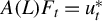. This is nonstandard because the vector $F_t$ has dimension r but is driven by $q<r$ shocks. Thus, the residual vector $u^*_t$ has rank q, so that $u^*_t=Q \tilde u_t$ , where $\tilde u_t$ is q-dimensional orthonormal white noise. This is not a big issue: in empirical situations, $r-q,$ eigenvalues of the covariance matrix are almost zero and a q-dimensional vector of residuals can easily be obtained. The big issue is that $\tilde u_t$ , being the residual of a VAR for $F_t$ , is fundamental for $F_t$ by definition, but, as we have argued before, there is no reason to assume that the structural $u_t$ is fundamental in $F_t= H(L) u_t$ .

An s-dimensional stochastic vector $Z_t$ driven by q shocks, with $q<s$ , is called dynamically singular. A dynamically singular vector has a singular spectral density at all frequencies. The covariance matrix of a dynamically singular vector is not necessarily singular. So the r-dimensional vector $F_t$ of static factors, which is driven by $q<r$ shocks, is dynamically singular.

In Forni et al. (Reference Forni, Giannone, Lippi and Reichlin2009)—this is joint work by Mario Forni, Domenico Giannone, myself, and Lucrezia Reichlin—we show that this dynamic singularity of the vector $F_t$ has an extremely important consequence: If you consider an s-dimensional vector which has a VARMA representation with a q-dimensional white noise, with $q<s$ , thus a dynamically singular VARMA, then generically, that is for all possible coefficients of the VARMA with negligible exceptions, the white noise is fundamental for $Z_t$ .

In our article, let me refer to it as the Black Box paper, we have this statement in a quite convoluted form. But when it was almost published, I got mail from Manfred Deistler with, in attachment, Anderson and Deistler (Reference Anderson and Deistler2008), along with a message asking “Did you know this?” Their paper contained a very elegant proof of the result I have just mentioned and much more: they proved that, generically, a dynamically singular VARMA has a finite AR representation. We were very happy: you see, we said, we are not wrong after all!

Let me only give you an example: you have $x_{1t}= u_t + 9 u_{t-1}.$ Of course, $u_t$ is not fundamental for $x_{1t}. $ Now suppose that you also observe $x_{2t}= u_t + 7 u_{t-1}.$ Again, $u_t$ is not fundamental for $x_{2t} $ . But if you take the vector $x_t=(x_{1t}\ x_{2t})$ , the scalar white noise $u_t$ is fundamental for $x_t$ . Multiply $x_{1t}$ by $-7$ , $x_{2t}$ by 9, and sum: you obtain $u_t$ as a linear combination of the x’s. You see that an additional variable makes up for the non-fundamentalness of $u_t$ for $x_{1t}$ . Provided, of course, that the additional variable does not contain an additional shock, bringing us back to the dynamically non-singular case. The same trick applies for any couple of MA(1) processes driven by the same $u_t$ , unless they have the same coefficient, so you see the genericity.

Lastly, as $\tilde u_t$ and $u_t$ are both orthonormal and fundamental for $F_t$ , $u_t=R \tilde u_t$ , with R orthogonal (this is a basic result in the theory of stationary stochastic processes). Determination of R is then obtained by standard Structural VAR techniques: you plug $F_t=A(L)^{-1 }Q \tilde u_t$ into $ \chi _{it} = C_{i1}F_{1t}+ \cdots + C_{ir} F_{rt}$ , then you impose, e.g., that the first shock has no long-run effect on the first variable in the dataset, which is income, the second shock has no contemporaneous impact on the second variable, etc. So the whole machinery is ready for empirical applications.

Quite an achievement: you have a solution to the aggregation and the fundamentalness problems. Now you know how to obtain the “true” macroeconomic variables and the number of variables you must use in a VAR to overcome the aggregation and fundamentalness problems. (MB, MD, MH)

To be precise, we have developed a method to estimate the structural shocks $u_t$ and impulse-response functions of the aggregate common components—the “true” macroeconomic variables—to $u_t$ . These impulse-response functions are the sum, or the mean, of the individual functions. We use no theory, nor any empirical knowledge, about such individual functions, their parameterization, etc.

But let us postpone further comments on Black Box and on some empirical work based on it to when we talk of a recent paper in which this idea of estimating VARs for the factors or the common components is pursued more systematically.

Here, I want to observe that our idea of “true variables,” as opposed to the observable variables, has a correspondence in the “concepts” of the dynamic stochastic general equilibrium (DSGE) models. The concepts, as they depend on a small number of structural shocks, are dynamically singular, just as our common components.

All right, but before the end of the first decade you also contributed to the construction of an indicator of real activity in the Euro Area. (MB, MD, MH)

This is an interesting application of the spectral approach. As is well known, you can define the business cycle within the GDP by band-passing the series at the business-cycle frequencies. However, and this is also well known, the band-pass filter is two-sided, so that at the end of the sample, it performs badly. In other words, using the band-pass filter, you do not get a reliable business-cycle component for the recent and current periods.

Frascati, Villa Mondragone, 1–4 October 2024. A workshop organized in honor of Marco Lippi’s 80th birthday; in the front row, from left to right, Marco Lippi, Jianqing Fan, Marc Hallin, and Masanobu Taniguchi.

In Altissimo et al. (Reference Altissimo, Cristadoro, Forni, Lippi and Veronese2010), Filippo Altissimo, Riccardo Cristadoro, and Giovanni Veronese, all at the Research Department of the Bank of Italy, in collaboration with Mario Forni and myself, produced a more reliable estimate of the business-cycle component for the current period by the following procedure:

1. (i) take a large dataset for the Euro Area, including the GDP;

2. (ii) estimate the spectral density of the common components;

3. (iii) cut the spectral density to keep only the business-cycle frequency band;

4. (iv) using such band-passed spectral density, estimate smooth factors with the generalized static principal component technique used in Forni et al. (Reference Forni, Hallin, Lippi and Reichlin2005);

5. (v) project the GDP on the smooth factors. You get a sort of smooth common component, which is our estimate of the band-pass filtered GDP.

Of course, our estimate is outperformed by the band-passed series for t far from the end of the sample. However, we find that it outperforms the band-passed series when t gets close to the end of the sample. So we use it as a coincident indicator of the business-cycle component of the Euro Area GDP, whence the acronym Eurocoin.

Eurocoin has been quite a success. It has been distributed monthly, starting at the beginning of the year 2000, by the Bank of Italy jointly with the Centre for Economic Policy Research (CEPR).Footnote ¹

8 RECENT WORK

Now, we are in the second decade and you get back to the general form of the model, without the static representation, and find at last a one-sided representation for the common components. (MB, MD, MH)

With the Black Box paper and the results by Anderson and Deistler in mind, I can easily give you a general idea about what we did.

1. (i) Forgetting about estimation issues, suppose that all the necessary covariances are known (again, structure theory, in the sense of Manfred Deistler). Using Brillinger principal components, which are based on the spectral density of the observable variables, the spectral density matrix of the n-dimensional vector of the common components $(\chi _{it})$ , $i=1,\ldots ,n$ of the Y’s can be obtained;

2. (ii) as we have the spectral density, and therefore all the necessary autocovariances, one may be tempted to compute the projections of the $\chi $ ’s on their lags. But this is exactly what cannot be done because of the curse of dimensionality with n and T tending to infinity together;

3. (iii) however, if we partition the n variables into subgroups of size $(q+1)$ (and assuming, for convenience, that n is a multiple of $(q+1)$ ), Anderson and Deistler ensure that generically each of the subgroups has a finite VAR representation; so we have an $n\times n$ VAR matrix, with $(q+1)\times (q+1)$ blocks on the main diagonal and zeroes elsewhere and, because the spectral density matrix of the $(\chi _{it})$ , $i=1,\ldots ,n$ is singular and has rank q at all frequencies, this block-diagonal matrix is a VAR matrix for $(\chi _{it})$ , $i=1,\ldots ,n$ .

This may be surprising: are we saying that the projection of $\chi _{1t}$ on the past of all the $\chi $ ’s is equal to the regression of $\chi _{1t}$ on the past of only the first $q+1$ ones? Yes, and this is the powerful consequence of dynamic singularity. Another way of saying the same thing is that the variables $\chi _{it-k}$ , $i=1,\ldots ,n$ and $k\in \mathbb N$ , are far from being linearly independent, as they are when the spectral density is non singular.

Further details would be very difficult to summarize in a few lines. Let me only add that the reason why we took so long to solve the two-sidedness issue was that we had missed the “blessing of dynamic singularity.” Thank you, Brian and Manfred!

These ideas are formally implemented in Forni et al. (Reference Forni, Hallin, Lippi and Zaffaroni2015) (i.e., Forni-Hallin-Lippi, with Paolo Zaffaroni replacing Lucrezia Reichlin, who was no longer interested in this research), in which we do the structure theory. Then, in Forni et al. (Reference Forni, Hallin, Lippi and Zaffaroni2017) we do the $(n, T)$ asymptotics, while the distributional theory is carried out in Barigozzi et al. (Reference Barigozzi, Hallin, Luciani and Zaffaroni2024).

And now we can use the spectral method for forecasting, which is what we did in Forni et al. (Reference Forni, Giovannelli, Lippi and Soccorsi2018), by Mario Forni, Alessandro Giovannelli, Stefano Soccorsi, and myself. Using the FRED database, we compared the forecast performance of our method with those of all other methods based on factor models, in particular Stock and Watson and also our 2005 FHLR method. The results were very good for the spectral method, though not spectacular.

So, I think we get to the point where we ask you what are your most recent works on macroeconometrics? (MB, MD, MH)

I think I would like to talk about four papers. Two of them belong to a project with Matteo Barigozzi and Matteo Luciani. We thought that I(1) variables and cointegration had not yet been treated in a fully satisfactory way in the literature on factor models. And I(1) is the rule, of course, with macroeconomic datasets, I(0) being the exception. One of our points was that dynamic singularity, which is the case with the static factors, implies a sort of trivial cointegration: the spectral density is singular at all frequencies and therefore at frequency zero. Cointegration and the Granger representation theorem in the case of I(1) dynamically singular vectors was the subject of Barigozzi, Lippi, and Luciani (Reference Barigozzi, Lippi and Luciani2020). Estimation in factor models when the variables are I(1) and the factors cointegrated is the subject of Barigozzi, Lippi, and Luciani (Reference Barigozzi, Lippi and Luciani2021).

And now let me do some showing off: Matteo Barigozzi, Alessandro Giovannelli, Matteo Luciani, Stefano Soccorsi, and Paolo Zaffaroni, whom I have just mentioned as coauthors, all of them have been more or less my students.

Third and fourth? (MB, MD, MH)

Talking about the Black Box paper, you said that Mario Forni and I had solved the aggregation problem we originally started with. Let me say that we gave a solution: of course, if you look into our papers, there are lots of linearities, assumptions, simplifications, etc. Together with Luca Gambetti and Luca Sala, we (Mario and I) recently published “Common Components Structural VARs (CC-SVAR)” (Forni et al., Reference Forni, Gambetti, Lippi and Sala2025a), a deeply revised version of the Black Box paper, where we carefully reconsider the issue of generic fundamentalness. Moreover, we relax a simplifying assumption that made the asymptotic analysis in Black Box extremely easy. Doing so, we discovered that dynamic singularity, after all, is not only a blessing!

The same paper also has a section in which we use the FRED dataset (McCracken and Ng, Reference McCracken and Ng2016) which I already mentioned to illustrate the advantages of CC-SVAR over standard SVAR analysis. We focus on monetary policy shocks. Our main results are: (I) As a consequence of non-fundamentalness and measurement errors, the results of the SVAR analysis are rather unstable, depending on (i) which variables are included in the SVAR vector and (ii) the identifying restriction employed. Thus, the conclusions on the effects of monetary policy shocks on macroeconomic variables are not robust. (II) Some improvement is obtained with FAVAR models, although the consequences of measurement errors are still evident. (III) With CC-SVAR, instability disappears and robust conclusions can be drawn. Independently of the choice of variables and identifying restrictions, contractionary monetary policy shocks reduce prices and economic activity. See also Forni and Gambetti (Reference Forni and Gambetti2010, Reference Forni and Gambetti2014) and Forni et al. (Reference Forni, Gambetti, Granese, Sala and Soccorsi2024) for empirical work based on Black Box and CC-SVARs.

Lastly, Forni et al. (Reference Forni, Gambetti, Lippi and Sala2025b). The main points of this article are:

1. (I) Structural VARs, estimated for the main macroeconomic variables, have been used as a data-based benchmark for evaluation of theory-based macroeconomic models.

2. (II) Based on Black Box and CC-SVARs, we make the ambitious claim that Structural VARs on the common components of the main macroeconomic variables— we call them CC-SVARs in the article—should rather be used as a benchmark for theory-based models, DSGE or Heterogenous Agents New Keynesian (HANK) models, in particular.

High time for conclusions … (MB, MD, MH)

I think there is a common thread in my research, starting with the Transformation Problem, running through Sraffa and leading to Aggregation in Econometrics and Factor Models. As I have already pointed out, when I started studying Sraffa I had already seen the failure of Marx’s attempt to measure aggregate capital with labor embodied. So when I found puzzling evidence in a relationship between aggregated time series I was immediately attracted to the aggregation problems in Granger and Morris.

Frascati, Villa Mondragone, 1–4 October 2024. A workshop organized in honor of Marco Lippi’s 80th birthday; from left to right, Masanobu Taniguchi, Marco Lippi, Esther Ruiz, Matteo Barigozzi, and Marc Hallin.

About aggregation in Econometrics, I would like to make another point. I do not think that scholars who use, more or less explicitly, the representative-agent fiction, really believe that all agents behave in the same way, with the same parameters. I think that they rather believe that agents’ heterogeneity is not a big issue after all: “Let us go on. We will make corrections afterwards, if necessary.” This is what Marx did, when he acknowledged that his solution of the Transformation Problem required corrections, but that these would be of minor importance. But an issue is of minor importance when you have proved that its consequences are negligible. Think of the stability problem in General Equilibrium Theory. Macroeconomists implicitly assume that this is a minor difficulty when they claim that their models possess a microfoundation. However, this is not the case as no general results on the stability of the General Equilibrium exist. On this point, see Kirman (Reference Kirman1992).

Anything more? (MB, MD, MH)

Yes. Recently I started a collaboration with Marco Magnani, an old friend and former student of mine (he attended my course on Piero Sraffa at the beginning of the 1970s in Rome, before Modena), who has been a prominent member of the Research Department at the Bank of Italy. We have produced a paper, still very tentative, on the theory of exploitation in the Marxist tradition and the modern Theory of Justice. The latter has set quite a rigorous and comprehensive framework to discuss inequality as a consequence of social origin, gender, race, etc. However, not all kinds of injustice are of the same importance and we believe that the role played by the individuals in the production of goods and services should be given back the centrality it used to have before the collapse of Real Socialism and the crisis of Social Democracy. But we can leave this for my 90th birthday’s interview (smile).

Vienna, 2024; from left to right, Philipp Gersing, Christoph Rust, Marco Lippi, and Manfred Deistler.

With Maria in Amsterdam (1991); Daria, Giordano, and Silvia.

You mentioned very little about your family life—your children and Maria. (MB, MD, MH)

Let me start by a recollection of my sister, Fiora Lippi. She was born in 1949 and suddenly died at the age of 22, when she had almost completed her graduation in Humanities. A loss that took a long time to come to terms with, especially for my parents.

About children, I am the proud father of three: Daria, who has been living in France for many years, is an actress and theater director. She founded a School for Theater Actresses and Actors at Bataville, Lorraine, where she collaborates with masters and researchers from other disciplines (other arts, sports, martial arts, ethology, neuroscience, …) to extract and formalize tools for acting. My son Giordano is an Associate Professor in the Department of Neuroscience at the Scripps Research Institute in San Diego, California, where he lives with Lorena Lee, an accomplished acupuncturist. Silvia is a teacher of yoga; recently, she started attending a laurea course in Law at the Catholic University in Milan, where she lives. I live with Maria Merelli, who has been a teacher of Italian and History in a High School in Modena. She is one of the founders of the Research Cooperative LeNove, whose main task is the study of public intervention, both in Italy and abroad, aimed at reducing gender inequality and fighting violence against women. They also contributed to the institution of an anti-violence public help-desk, which is currently active in Italy. In the years 1990–1995, she served as a deputy in the regional Parliament of Emilia-Romagna. Both she and I have a divorce in our past. She has three children, Cecilia, Alberto, and Filippo Della Casa, so we have a total of six.