1. Prediction of turbulent flow characteristics over rough walls

Predicting roughness effects on near-wall turbulence remains a topic of paramount practical importance, since most engineering-relevant flows are turbulent, most surfaces are not hydrodynamically smooth, and the influence of roughness on engineering quantities (e.g. drag) may be significant. Despite sustained interest in the topic, many methods of quantifying the effects of roughness on wall turbulence remain at least semiempirical, relating predominantly to global statistics of the roughness geometry. In this work, we provide a framework by which to understand flow sensitivity and turbulent response to specific scales of roughness, the development of dispersive stresses and their feedback on the mean velocity (figure 1 a). The end result is the iterative loop relating a scan of roughness geometry to the associated mean flow response shown in figure 1(b) (Chan Reference Chan2024).

In many complex, high-Reynolds-number engineering-relevant flows with flow over fully developed rough walls, the representative geometric roughness scale, for example the sandgrain roughness height, $k$ , is small with relation to the outer flow scale, $\delta$ . Besides an increase in the drag at the wall due to the presence of the roughness, and therefore an increase in the friction velocity, $u_\tau$ , the direct effect of roughness in this regime is generally confined to the roughness sublayer, a region which extends from the wall $y = 0$ to $y \approx (3-5)k$ . By Townsend’s hypothesis, flow outside of the roughness sublayer reflects the changed $u_\tau$ , but otherwise retains the similarity characteristics of a smooth wall at the same friction Reynolds number, $\textit{Re}_\tau = \delta ^+ = \delta u_\tau /\nu$ , where $\nu$ is the kinematic viscosity. The global effects of roughness on the mean velocity field and drag are encapsulated by the equivalent sandgrain roughness $k_s^+$ and Hama roughness-function $\Delta U^+$ , which are fundamentally due to the spatially varying modulation of the near-wall turbulence by the surface roughness and the introduction of drag forces on the roughness elements.

Many efforts to model turbulence over realistic, multiscale surface geometries bypass the details of the spatially varying roughness sublayer fluctuations and focus instead on directly predicting $k_s^+$ and/or $\Delta U^+$ given averaged statistics and spectral information about the roughness using empirical models. The literature is broad and has been recently reviewed by Flack & Chung (Reference Flack and Chung2022). One especially effective physics-based effort is the wind-shade model of Meneveau et al. (Reference Meneveau, Hutchins and Chung2024) which uses minimal empirical assumptions to link surface features of realistic roughness to the resulting drag. In a paper of direct relevance to the present work, Mejia-Alvarez & Christensen (Reference Mejia-Alvarez and Christensen2010) demonstrated that low-order representations of roughness on a wind turbine surface produced similar stresses to the full surface geometry, indicating that only certain geometric scales contribute to the drag response or, equivalently, that the flow sensitivity is roughness-scale-dependent. It remains desirable to seek model forms that more directly encode the physics linking roughness features to the drag response through modelling the roughness sublayer fluctuations and their spatially varying effects.

Here we introduce resolvent analysis with volume penalization (RAVP). The efficacy of the RAVP modelling framework is tested using the direct numerical simulation (DNS) of a channel flow over sandgrain roughness in the fully rough regime conducted by Hantsis & Piomelli (Reference Hantsis and Piomelli2020). Full details of the solution, which uses a second-order accurate central difference in space on a staggered mesh and a second-order accurate semi-implicit time advancement method may be found therein; we summarize the simulation conditions in table 1. Sandgrain roughness consisting of randomly oriented ellipsoids with semiaxes  $k$ , $1.4k$ and $2k$ , where $k = 0.04\delta$ , is modelled symmetrically on both walls using the immersed boundary method (IBM). In the fully rough regime, $k_s \approx 1.6k$ for this geometry. The simulation is run at a constant $\textit{Re}_b = 21{\,}400$ and temporal averages are computed over 50 eddy turnover times.

2. A drag-scaled, Re-decomposed volume penalization in resolvent analysis

Resolvent analysis provides a method to predict the modal structure that is most amplified by the Navier–Stokes operator linearized relative to the mean field. The method has been extensively documented in the literature, e.g. McKeon (Reference McKeon2017), thus we describe here the modified RAVP. We use RAVP to obtain a transfer function relating velocity response in the form of modes describing the wake field, or the zero frequency variations from the spatially averaged velocity fields, to roughness geometry, given a mean flow profile and a surface scan of an engineering-relevant roughness. We note that other authors have considered related resolvent-based approaches of non-spatially uniform boundary conditions, including rough walls that can be well described by a single wavenumber and its harmonics via the solution of wavenumber-coupled resolvent systems. In particular, for riblet surfaces Chavarin & Luhar (Reference Chavarin and Luhar2020) developed a volume penalization method using a permeability function to drive the flow velocity to zero in the solid region and Flynn et al. (Reference Flynn, Bae and Goza2024) developed a projection-based immersed boundary method and applied it to a sinusoidal roughness.

Table 1.

Numerical domain $(L_x, L_y, L_z)$ and simulation parameters (top line) and RAVP-M predictions after $N_{eval} = {162}$ iterations through the loop of figure 1(b).

Table 1. Long description

A table comparing numerical domain and simulation parameters for DNS and RAVP-M. The table has 2 rows and 14 columns. Column headers are: Reτ, uτ/Ub, ΔU+, k+ s, k/δ, Lx/δ, Ly/δ, Lz/δ, Nx, Ny, Nz, Δx+, Δy+min, Δz+. Row 1: DNS, 1745, 0.0814, 9.2, 112, 0.04, 6, 2.064, 3, 1024, 530, 512, 10.2, 0.84, 10.2. Row 2: RAVP-M, 1739, 0.0813, 9.3, 114, -, -, -, -, -, -, -, -, -, -.

Figure 1.

(a) An input–output framework relating surface-specific roughness geometry input at a given flow condition, here specified by bulk Reynolds number, $\textit{Re}_b$ , to the corresponding global (averaged) and local (spatially varying) flow features using RAVP and a mean flow model. (b) Iterative loop of RAVP coupled to the mean momentum balance (MMB) to recover the mean velocity profile, which we identify as RAVP-M.

We consider the continuity equation and the momentum equations for incompressible turbulent channel flow of a Newtonian fluid augmented by a forcing term that accounts for the presence of the roughness, $-\boldsymbol{F}^{\textit{RA}}$ :

(2.1) \begin{align} \frac {\partial \boldsymbol{u}}{\partial t} + \boldsymbol{u} \boldsymbol{\cdot }\boldsymbol{\nabla }\boldsymbol{u} &= -\boldsymbol{\nabla }p + \frac {1}{\textit{Re}_\tau } {\nabla} ^2 \boldsymbol{u} - \boldsymbol{F}^{\textit{RA}},\nonumber\\ \boldsymbol{\nabla }\boldsymbol{\cdot }\boldsymbol{u} &= 0. \end{align}

A triple decomposition is used to identify the intrinsic spatiotemporal average, $\langle \overline {q}\rangle (y)$ , the wake field, $\tilde {q}(x,y,z)$ , and the spatially and temporally varying component, $q'(x,y,z,t)$ ,

(2.2) \begin{align} q(x,y,z,t) = \langle \overline {q}\rangle (y) + \tilde {q}(x,y,z) + q'(x,y,z,t). \end{align}

For flow quantities, the intrinsic average $\left \langle \,\boldsymbol{\cdot }\, \right \rangle$ is calculated at each $xz$ -plane as the average of the quantity over the fluid-occupied area, and is used in the triple decomposition to define the wake field. The area fraction occupied by fluid is denoted $\varPhi (y)$ , and is calculated as the plane average of the volume of fluid fraction (VOF) $\varphi (x,y,z)$ . The superficial average $\left \langle \,\boldsymbol{\cdot }\, \right \rangle _s$ is calculated by summing the quantity over the fluid-occupied area and dividing by the full plane area, and is related to the intrinsic average by $\left \langle \,\boldsymbol{\cdot }\, \right \rangle _s = \varPhi \left \langle \,\boldsymbol{\cdot }\, \right \rangle$ . We use a strict VOF representation, where any cell with $\varphi \lt 1$ is set to $\varphi = 0$ , such that when a spatial (plane) average is taken over a fluid quantity, denoted by $\langle {\,\boldsymbol{\cdot }\,}\rangle _{xz}$ , multiplied by $\varphi$ , only data in cells which do not contain any of the solid are considered (effectively a low-pass spatial filter). The plane average $\left \langle \,\boldsymbol{\cdot }\, \right \rangle _{xz}$ is calculated as the sum of a quantity over the full plane area, divided by the full plane area. The plane and superficial averages are equal when the quantity is equal to zero within the fully roughness-occupied area.

The (spatially varying) force, $\boldsymbol{F}^{\textit{RA}}$ , reflects the roughness geometry, and is of the same form as the IBM forcing, i.e.

(2.3) \begin{align} {F}^{\textit{RA}}_i(x,y,z) = Du_i= [1{\kern-1pt}-{\kern-1pt}\varphi (x,y,z)] D_{\textit{max}}u_i,\, F^{\textit{IBM}}_i(x,y,z) = -[1{\kern-1pt}-{\kern-1pt}\varphi (x,y,z)]\frac {1}{\Delta t^n}u_i. \end{align}

Here subscript $i$ and $\Delta t^n$ denote the $i$ th component and $n$ th time step, respectively. Here ${F}^{\textit{RA}}_i$ depends on the roughness geometry expressed in terms of the VOF and a real-valued magnitude parameter $D_{\textit{max}}$ , which is closed to normalize the integral of the drag term using the mean streamwise momentum equation computed by plane averaging,

(2.4) \begin{align} \frac {1}{\textit{Re}_\tau }\frac{\textrm {d}\left \langle \overline {u} \right \rangle _s}{\textrm {d} y} - \langle \overline {u'v'} \rangle _s - \left \langle \tilde {u}\tilde {v} \right \rangle _s {+} \int _y^1 \left \langle D\overline {u} \right \rangle _{xz} {\rm d}y' = {1-y}, \end{align}

(2.5) \begin{align} \int _0^1 \left \langle D\overline {u} \right \rangle _{xz} {\rm d}y' = D_{\textit{max}} \int _{0}^1 \left [ \left \langle 1-\varphi \right \rangle _{xz}\left \langle \overline {u} \right \rangle _s - \left \langle \tilde {\varphi }\tilde {u} \right \rangle _{xz} \right ] {\rm d}y' = 1. \end{align}

The time average (indicated here by an overline), stochastic fluctuations and $\tilde {v}$ have zero value in the roughness sublayer for a channel flow. Thus, plane averages and superficial averages are equivalent for the temporally averaged $\overline {u}$ , the stochastic stress $\overline {u'v'}$ and the dispersive stress $\tilde {u}\tilde {v}$ . Assuming that $\left \langle \tilde {\varphi }\tilde {u} \right \rangle _{xz}$ is small (since it is the product of two spatial variations), a scalar $D_{\textit{max}}$ can be determined. Or, utilizing the form of the IBM force in the simulation, which corrects the velocity to zero inside of the roughness, a wall-normally varying function $\mathcal{D}_{\textit{max}}(y)$ which matches the equivalent IBM force profile $\big \langle \overline {F^{\textit{IBM}}_1} \big \rangle _{xz}$ , may also be determined for comparison with the scalar $D_{\textit{max}}$ ,

(2.6) \begin{align} D_{\textit{max}} = \frac {1}{\int _0^1 \left \langle 1-\varphi \right \rangle _{xz}\left \langle \overline {u} \right \rangle _s{\rm d}y'}, \hspace {5mm} \mathcal{D}_{\textit{max}}(y) = -\frac {\big \langle \overline {F^{\textit{IBM}}_1} \big \rangle _{xz}}{\left \langle 1-\varphi \right \rangle _{xz}\left \langle \overline {u} \right \rangle _s}. \end{align}

Both drag models provide reasonable agreement with the true IBM force (figure 2 a), however, the scalar $D_{\textit{max}}$ may be used without having completed an IBM simulation. Under these assumptions, the drag force profile is approximated as $\left \langle D\overline {u} \right \rangle _{xz} \approx \left \langle D \right \rangle _{xz}\left \langle \overline {u} \right \rangle _s$ .

Figure 2.

(a) Forcing in (2.1): RAVP with a scalar $D_{\textit{max}}$ shows good agreement with the plane-averaged drag term from the IBM simulation (data) and RAVP with $\mathcal{D}_{\textit{max}}(y)$ tuned to match the IBM force. (b,c) RAVP improves the agreement between the shape of the first resolvent response modes and DNS wake field modes (data) relative to traditional resolvent analysis using smooth wall (RA-s) and true rough wall (RA-r) mean profiles for $u$ and $v$ , respectively, from a sample mode with $(\lambda _x^+, \lambda _z^+) = (1047, 436)$ . (d) Spectrum of the projection coefficient for the wake field data onto the first symmetric RAVP mode. The overlaid contour indicates where the wake field turbulent kinetic energy (TKE) is $10\,\%$ of its maximum. (e) Spectrum of the weights $\chi _{\boldsymbol{k},1}$ computed from (2.8) which includes all forcing inputs to the resolvent operator. (f) Spectrum of the weights $\chi _{\boldsymbol{k},1}$ for the compressed model computed using (2.9) which only includes the linear forcing term $-\hat {D}_{\boldsymbol{k}}\langle \overline {\boldsymbol{u}}\rangle _s$ .

By Reynolds decomposing the volume penalized drag term as well as the turbulent state relative to the plane average, and denoting the Fourier-transformed state at a given streamwise wavenumber, spanwise wavenumber and temporal frequency triplet, $\boldsymbol{k} = (k_x, k_z, \omega )$ , by $\hat {\boldsymbol{\cdot }}$ , we obtain an expression for the modified resolvent operator,

(2.7) \begin{align} \begin{bmatrix} \hat {\boldsymbol{u}}_{\boldsymbol{k}} \\ \hat {p}_{\boldsymbol{k}} \end{bmatrix} = {\left (-i\omega \begin{bmatrix} \boldsymbol{I} & \\ & 0 \end{bmatrix} - \begin{bmatrix} \boldsymbol{\mathcal{L}_k} - \textit{diag}\left \langle D \right \rangle _{xz} & -\boldsymbol{\nabla }\\ {\nabla} ^{\top } & 0 \end{bmatrix} \right )^{-1}} \left (\kern0.5pt\hat {\kern-2.5pt\boldsymbol{f}}_{\!\boldsymbol{k}} - \hat {D}_{\boldsymbol{k}}\left \langle \overline {\boldsymbol{u}} \right \rangle _s + \kern0.5pt\hat {\kern-2.5pt\boldsymbol{d}}_{\kern-1pt\boldsymbol{k}}\right ). \end{align}

Here $\mathcal{L}_k$ is the usual linearized Navier–Stokes operator (linearized relative to the superficial mean velocity), $\boldsymbol{\nabla}$ is the gradient, $N_y$ is the number of discretization points in the wall-normal direction, and zero mean wake velocities, $\left \langle \overline {v} \right \rangle _s$ and $\left \langle \overline {w} \right \rangle _s$ , are assumed. Standard channel flow boundary conditions are used here, i.e. the boundary conditions are not modified by the roughness geometry. Relative to the classical, smooth wall analysis, the resolvent is modified directly by the plane-averaged drag force, $\textit{diag}\left \langle D \right \rangle _{xz}$ . With $\boldsymbol{u}''= \tilde {\boldsymbol{u}}+\boldsymbol{u}'$ , two additional forcing terms beyond the usual nonlinear interaction of velocity fluctuations $\kern0.5pt\hat {\kern-2.5pt\boldsymbol{f}}_{\!\boldsymbol{k}} = - ({\boldsymbol{u}''\boldsymbol{\cdot }\boldsymbol{\nabla }\boldsymbol{u}'' - \langle \overline {\boldsymbol{u}''\boldsymbol{\cdot }\boldsymbol{\nabla }\boldsymbol{u}''}\rangle _{xz}} )_{\boldsymbol{k}}$ represent (i) the coupling between the roughness and the superficial mean flow ( $\hat {D}_{\boldsymbol{k}}\left \langle \overline {\boldsymbol{u}} \right \rangle _s$ ) and (ii) nonlinear interactions between the spatially varying $\hat {D}_{\boldsymbol{k}}$ and spatially and temporally varying velocity modes, $\kern0.5pt\hat {\kern-2.5pt\boldsymbol{d}}_{\kern-1pt\boldsymbol{k}} = - (\tilde {D}{\boldsymbol{u}''} - \langle {\tilde {D}\tilde {u}\rangle _{xz}} )_{\boldsymbol{k}}$ . The full state may be expanded in the usual way in terms of a weighted singular value decomposition of the resolvent, ${\mathcal{H}_{\boldsymbol{k}}} = \sum _{j=1}^N {\sigma }_{\boldsymbol{k},j} {\psi }_{\boldsymbol{k},j}{\phi }_{\boldsymbol{k},j}^{\dagger }$ , i.e.

(2.8) \begin{align} \begin{bmatrix} \hat {\boldsymbol{u}}_{\boldsymbol{k}} \\ \hat {p}_{\boldsymbol{k}} \end{bmatrix} &= {\mathcal{H}_{\boldsymbol{k}}} \left ( \kern0.5pt\hat {\kern-2.5pt\boldsymbol{f}}_{\!\boldsymbol{k}} - \hat {D}_{\boldsymbol{k}}\left \langle \overline {\boldsymbol{u}} \right \rangle _s+\kern0.5pt\hat {\kern-2.5pt\boldsymbol{d}}_{\kern-1pt\boldsymbol{k}} \right ) \nonumber\\& = \sum _{j=1}^N {\sigma }_{\boldsymbol{k},j} {\psi }_{\boldsymbol{k},j} {\chi }_{\boldsymbol{k},j} \quad \text{with} \quad {\chi }_{\boldsymbol{k},j} = \big \langle {\phi }_{\boldsymbol{k},j}, \kern0.5pt\hat {\kern-2.5pt\boldsymbol{f}}_{\!\boldsymbol{k}} - \hat {D}_{\boldsymbol{k}}\big \langle \overline {\boldsymbol{u}} \big \rangle _s + \kern0.5pt\hat {\kern-2.5pt\boldsymbol{d}}_{\kern-1pt\boldsymbol{k}}\big \rangle . \end{align}

Here $\hat {D}_{\boldsymbol{k}}\left \langle \overline {\boldsymbol{u}} \right \rangle _s$ is already known and non-zero only for wake field fluctuations, which have $\omega = 0$ . The interaction between the turbulent fluctuations and spatial variation of the roughness geometry, $\kern0.5pt\hat {\kern-2.5pt\boldsymbol{d}}_{\kern-1pt\boldsymbol{k}}$ , is not known $\textit{a priori}$ but is assumed to be small, such that the forcing in the roughness sublayer is dominated by the wall boundary condition via the drag model, and the weights on the resolvent forcing modes are determined using

(2.9) \begin{align} {{\chi }}_{\boldsymbol{k},j} \triangleq \big \langle {\phi }_{\boldsymbol{k},j}, -\hat {D}_{\boldsymbol{k}}{\left \langle \overline {\boldsymbol{u}} \right \rangle _s}\big \rangle . \end{align}

We consider first the ability of RAVP to capture an efficient representation of amplified wake field modes, for which $\omega =0$ by construction and thus the resolvent in (2.7) could be modified accordingly. The resolvent operators are computed on an $N_y=200$ point Chebyshev grid defined on $y_{cheb} \in [-1,1]$ and we calculate and use 25 of the leading symmetric resolvent modes for modelling. Since resolvent modes with support restricted to the near wall region appear in symmetric and antisymmetric pairs, the symmetric modes are sufficient to describe the effect of roughness that is mirrored on the top and bottom walls. Comparison of the streamwise and wall-normal velocity components of a representative wake field mode from the DNS with the leading (first) resolvent mode obtained from RAVP using the plane-averaged mean field (figures 2 b and 2 c) shows associated improvement in agreement between the location of the peak amplitude for RAVP modes and data relative to classical (non-drag-modified) resolvent analysis using either the relevant smooth or rough wall means. These panels effectively isolate the influence of the drag modified operator (i.e. (2.7)); the influence of the forcing model in (2.9) is additionally considered when integrated across scales in figure 3. Further, the normalized projection of the DNS wake field data onto the first symmetric RAVP response mode is high in the region where the TKE of the wake field is significant, shown in figure 2(d) (for this roughness, confined to the lowest values of streamwise and spanwise wavenumbers).

Turning to the nonlinear forcing, the associated spectrum of the nonlinear weights on the first resolvent modes, ${{\chi }}_{\boldsymbol{k},1}$ (2.8), is shown in figure 2(e). The most active modes lie in a similar wavenumber range to the response, with differences due to the relative gains of each mode, which is encapsulated in the variation of ${\sigma }_{\boldsymbol{k},1}$ with $\boldsymbol{k}$ . We further compress the RAVP representation of the roughness following the insight of Mejia-Alvarez & Christensen (Reference Mejia-Alvarez and Christensen2010) by low-pass filtering the Fourier representation of the roughness geometry from a total of $N_{k_x} \times N_{k_z} = 512 \times 256$ wavenumbers, to a subset consisting of the lowest $64 \times 128$ wavenumbers (justified for this roughness with reference to figure 2 d). The associated distribution of weights computed from this reduced set of wavenumbers and the linearized forcing model of (2.9) is given in figure 2(f).

Figure 3.

(a) Comparison of the wake field from (i,iv,vii) the data, (ii,v,viii) the model reconstruction and (iii, vi,ix) the compressed model. From (i–iii) to (vii–ix), streamwise, wall-normal and spanwise velocity components at $y/\delta = 0.03$ are shown. Black lines show the location of the edges of the (full) roughness geometry in this plane. (b) Wall normal variation of the dispersive stresses from data, model reconstruction and compressed model.

The impact of the filtering is not negligible in terms of comparison of the compressed RAVP model with the DNS wake field or the full RAVP reconstruction, which is able to capture the velocity variations with reasonable fidelity (figure 3 a). Similarly, while the normal dispersive stresses in figure 3(b) are not very well captured by the compressed RAVP (wall-normal in particular), the dispersive shear-stress profile is reasonable, suggesting that key correlations between velocity components are retained. The wake fields underscore the origin of the latter point. While compressed RAVP preferentially weighs large wavelength fluctuations in the roughness sublayer, the phase relationships between velocity components across all scales are such that the dispersive shear-stress is reasonably preserved and a substantially simplified model for the response of the flow to the varying roughness geometry can be obtained.

3. Iteration for the mean flow and wake field: prediction of turbulent flow response

The dispersive stresses obtained using compressed RAVP for a given roughness geometry and an estimate of the mean velocity profile are now employed in an iterative loop, which we deem RAVP-M, to determine the true mean-velocity profile, figure 1(b). The mean streamwise momentum equation for a rough wall requires consideration of the drag force due to the roughness, $F_D$ , the rough wall stochastic stress as well as the dispersive stress,

(3.1) \begin{align} {\frac{\textrm {d}}{\textrm {d} y}}\left [\frac {1}{\textit{Re}_\tau }{\frac {\textrm {d} \langle \overline {u} \rangle _s}{\textrm {d} y}} - \big \langle \overline {u'v'} \big \rangle _s - \left \langle \tilde {u}\tilde {v} \right \rangle _s\right ] + F_D = {-1}, \end{align}

as shown in figure 4(a). The drag force $F_D$ , which represents the plane-average of viscous and pressure forces on the roughness elements, can be modelled based on the mean momentum forcing term from RAVP,

(3.2) \begin{align} F_D(\left \langle \overline {u} \right \rangle _s, \varphi ) = -{\left \langle D \right \rangle _{xz}}\left \langle \overline {u} \right \rangle _s \!, \end{align}

where we use the scalar $D_{\textit{max}}$ of (2.6). As noted above, this term can be cheaply evaluated given only the mean velocity profile.

Figure 4.

(a) The iterative mean flow model converges the components of the mean flow balance towards the true (DNS data) variations. (b) After $N_{eval} = {162}$ iterations and initialization with the smooth wall profile (shown in blue), the model mean flow profile (dashed red line) has converged well to the true rough wall profile (solid red line).

We use a modified eddy viscosity profile, $\nu _{T_r}(y)$ , to model the superficial average of the stochastic Reynolds stress, $\big \langle \overline {u'v'} \big \rangle _s$ . Here $\nu _{T_r}(y)$ is monotonically attenuated from the equivalent smooth wall value, $\nu _T(y)$ (obtained using the Cess model with parameters $\kappa = 0.426$ and $B = 25.4$ (Del Álamo & Jiménez Reference Del Álamo and Jiménez2009)), at the top of the roughness sublayer to zero at $y=0$ using a piecewise continuous function, $\zeta (F_D)$ , such that

(3.3) \begin{align} \nu _{T_r} = (1-\zeta (F_D))\nu _T, \hspace {5mm} \zeta (F_D) = {g}(y;y_0,\gamma ) = \frac {1}{1+\left (\frac {y-y_0}{C{\gamma }}\right )^2}. \end{align}

A Cauchy function constructed to peak at the walls and provide wall-normal support in agreement with the wall-normal extent of the drag force $F_D$ is selected for $\zeta ({F_D})$ . Here $y_0$ denotes the peak location, and $\gamma$ is the scale parameter which specifies the half-width at half-maximum of the normalized Cauchy function. The values of $C$ and $\gamma$ together define the attenuation of the eddy viscosity expected in the presence of roughness. A (constant) value of $C = 3.04$ is found to be suitable for describing the behaviour of the rough wall eddy viscosity (figure 4 a); this is analogous to the depth of the roughness sublayer. At a given iteration $i$ , $\gamma$ is defined based on the best fit to the shape of $F_D$ . While it would be possible to use different functions, $\hat {\zeta }(F_D)$ , for the top and bottom of the channel, here the functional form remains the same since each wall has identical roughness statistics.

The solution for the mean flow is now iterative, as laid out in figure 1(b), with inputs of the surface roughness geometry, $k(x,z)$ , and an initial guess for the inner-scaled mean flow profile $\left \langle \overline {u} \right \rangle _s^{(i)}$ at the desired bulk Reynolds number $\textit{Re}_b^{\textit{desired}}$ . RAVP gives predictions for the drag force and dispersive stress, then the MMB is solved to give a new inner-scaled mean profile, $\left \langle \overline {u} \right \rangle _s^{(i+1)}$ . From this mean profile, $u_\tau ^{(i+1)}$ , a new $\textit{Re}_b^{(i+1)}$ and a new $\textit{Re}_\tau ^{(i+1)}$ , if needed, are computed using

(3.4) \begin{align} u_\tau ^{(i+1)} &= \frac {1}{\int _0^1 \left \langle \overline {u} \right \rangle _s^{(i+1)}{\rm d}y}; \, \textit{Re}_b^{(i+1)} = \frac {\textit{Re}_\tau ^{(i)}}{u_\tau ^{(i+1)}}; \nonumber\\ \textit{Re}_\tau ^{(i+1)} &= \textit{Re}_\tau ^{(i)} + \left (\textit{Re}_b^{(i+1)}-\textit{Re}_b^{\textit{desired}}\right )u_\tau ^{(i+1)}. \end{align}

The equations are discretized and solved using Chebyshev differentiation matrices (Weideman & Reddy Reference Weideman and Reddy2000). The iteration is initialized using the smooth-wall mean profile for the $\textit{Re}_b$ of interest as a readily available initial guess for the velocity field and zero dispersive stress. Compressed RAVP for the dispersive stress is first evaluated at the second iteration to allow the mean profile shape to be somewhat corrected by the drag term and adjusted eddy viscosity during the first step, which leads to a better estimate for the dispersive stress, and then again every $N_{update}$ iterations to reduce cost while still encoding the relationship between the mean flow profile and dispersive stress. 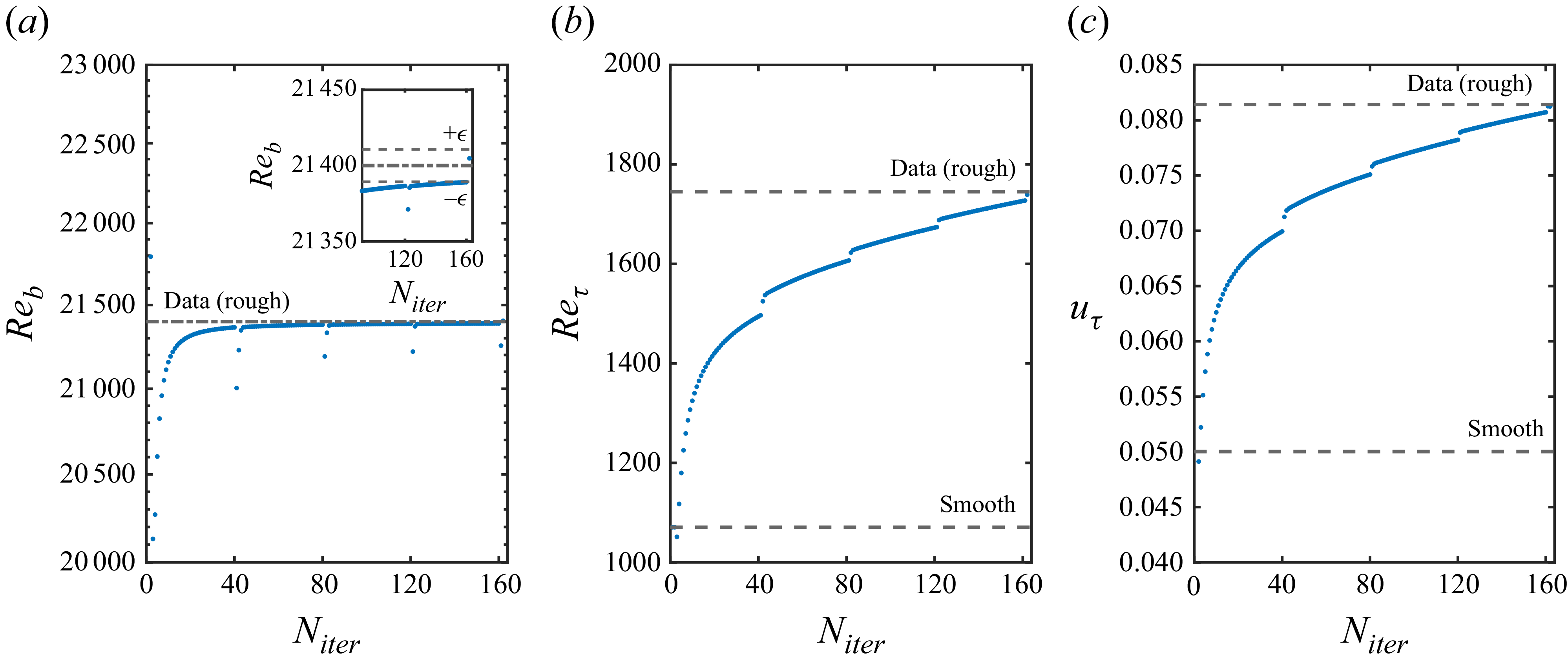Iteration through this loop continues until the resulting bulk Reynolds number matches the desired bulk Reynolds number to a chosen error, ${|\textit{Re}_b^{(i+1)} - \textit{Re}_b^{\textit{desired}}|} \lt \epsilon \,{\textit{Re}_b^{\textit{desired}}}$ for a given choice of $\epsilon$ , a user selected error tolerance on the bulk Reynolds number. The resulting evolution of the values of $\textit{Re}_b$ , $\textit{Re}_\tau$ and $u_\tau$ is plotted in figure 5(a–c). All these quantities converge monotonically towards the true values, where the discontinuities correspond to where the dispersive stress is updated, however, the stopping criterion is based on the error tolerance for the bulk Reynolds number for consistency with the conditions that are used as input to RAVP-M. Here $\Delta U^+$ and $k_s^+$ are evaluated using the average deviation of the mean velocity from a log law with smooth wall constants $\kappa = 0.39$ and $B=5$ over $y^+ \in [3\textit{Re}_\tau ^{0.5}, 0.15\textit{Re}_\tau ]$ , and the fully rough relationship between them with $D_r=7.9$ , which is in the range observed for most rough wall surfaces:

(3.5) \begin{align} k_s^+ = \exp \left [\kappa (\Delta U^+ -B+D_r)\right ]. \end{align}

We used iteration parameters $\epsilon = 0.0005$ , $N_{update} = 40$ and $N_{eval} = 162$ to obtain the results in figure 4(a,b) in approximately 2 hours.

Figure 5.

(a) The $\textit{Re}_b$ evolution with iteration number. The inset depicts the final convergence to within the $\epsilon$ bounds. (b) The $\textit{Re}_\tau$ evolution with iteration number. (c) The $u_\tau$ evolution with iteration number.

The modelled MMB terms closely approximate those from the DNS, with a slight underestimation of the mean flow gradient within the roughness geometry. The dispersive stress is underestimated because the model for the weights $\chi _{\boldsymbol{k},j}$ in (2.9) underestimates streamwise wake field fluctuations at $y/\delta \lt 0.05$ , as illustrated earlier in figure 3(b). The drag force is slightly overestimated, which is characteristic of the RAVP analysis, while the stochastic stress agrees well with the data. Nonetheless, the RAVP-M rough wall mean velocity (figure 4 b) agrees well with the DNS, with minor differences observed deep into the roughness, well below the roughness crest. The computed values of friction Reynolds number, $\Delta U^+$ and $k_s^+$ are shown in table 1. Here $\textit{Re}_\tau$ is recovered within $0.4\,\%$ accuracy, while the evaluations of Hama roughness factor and equivalent sandgrain roughness, which depend on the precise definitions employed to determine them, are also within $2\,\%$ of the DNS values.