1 Introduction
In this paper we report on a computational study of turbulent heat transfer in liquid–liquid flows in a T-junction. More specifically, we present results from a direct numerical simulation (DNS), and a wall-resolved large-eddy simulation (LES), of the interaction between a hot horizontal cross-flow and a cold vertical jet coming from above, in a T-junction of rectangular cross-section. Due to their mixing efficiency, T-junctions constitute a principal component of hydraulic and pneumatic circuits and they are encountered in numerous applications, such as HVAC (heating, ventilation and air-conditioning) systems, intake manifolds of internal combustion engines, cooling systems of nuclear reactors and others. Because of their wide applicability, several research efforts have been dedicated to their study thus far.
As regards recent experimental investigations, Kamide et al. (Reference Kamide, Igarashi, Kawashima, Kimura and Hayashi2009) and Walker et al. (Reference Walker, Simiano, Zboray and Prasser2009) examined the effect of different momentum ratios between the two streams on the thermal mixing in T-junctions with circular cross-sections. Also, Kuschewski, Kulenovic & Laurien (Reference Kuschewski, Kulenovic and Laurien2013) carried out experiments in horizontal T-junctions, i.e. with the gravity vector pointing to the spanwise direction, with circular cross-sections and at high ambient pressure so as to match the working conditions in liquid water reactors. Further, various authors conducted experiments in rectangular T-junctions at different Reynolds numbers and momentum ratios; see, e.g. Hirota et al. (Reference Hirota, Asano, Nakayama, Asano and Hirayama2006, Reference Hirota, Mohri, Asano and Goto2010), de Tilly & Sousa (Reference de Tilly and Sousa2008), Naik-Nimbalkar et al. (Reference Naik-Nimbalkar, Patwardhan, Banerjee, Padmakumar and Vaidyanathan2010) and the more recent paper of Lin, Chen & Ferng (Reference Lin, Chen and Ferng2016).
Additionally, several computational efforts have been devoted to turbulent heat transfer in T-junctions. Due to the high computational cost of DNS, all the currently available studies have been based on LES. For example, Hu & Kazimi (Reference Hu and Kazimi2006) performed one of the first simulations of this type, followed by Lee et al. (Reference Lee, Hu, Saha and Kazimi2009), Kuczaj, Komen & Loginov (Reference Kuczaj, Komen and Loginov2010), Kuhn et al. (Reference Kuhn, Braillard, Ničeno and Prasser2010), Lu et al. (Reference Lu, Jiang, Guo, Zhang and Li2010). However, those early studies employed rather coarse grids with respect to the Reynolds number of the flow.
Subsequently, the appreciation of the complexity of the flow of interest, supported by the ever-increasing computational resources, prompted researchers to employ finer grids in their simulations. For example, Sakowitz, Mihaescu & Fuchs (Reference Sakowitz, Mihaescu and Fuchs2013, Reference Sakowitz, Mihaescu and Fuchs2014) performed LES of flows in both circular and rectangular T-junctions and at Reynolds numbers of the order of 10 000. These authors reported that, in both geometries, the shear layer that is formed between the jet and the cross-flow oscillates with a Strouhal number of order one. Also, based on the their LES study, Howard & Serre (Reference Howard and Serre2015, Reference Howard and Serre2017) concluded that mixing is enhanced by the horseshoe and counter-rotating vortices that are formed near the entry of the incoming jet. Further, Selvam, Kulenovic & Laurien (Reference Selvam, Kulenovic and Laurien2015), Gauder et al. (Reference Gauder, Selvam, Kulenovic and Laurien2016) and Kickhofel et al. (Reference Kickhofel, Prasser, Selvam, Laurien and Kulenovic2016) replicated via LES the aforementioned experiments of Kuschewski et al. (Reference Kuschewski, Kulenovic and Laurien2013). Nonetheless, the aforementioned simulations did not resolve the near-wall regions, but instead relied on wall models.
However, there is significant evidence that wall models do not perform well in separation regions and, generally, in regions with adverse or favourable pressure gradients; see, for example, the relevant discussions by Jayaraju, Komen & Baglietto (Reference Jayaraju, Komen and Baglietto2010) and Tunstall et al. (Reference Tunstall, Laurence, Prosser and Skillen2016a ). For this reason, the focus of recent studies has been shifted toward wall-resolved LES. For example, Tunstall et al. (Reference Tunstall, Laurence, Prosser and Skillen2016b ) performed such simulations for T-junctions with an upstream elbow at a Reynolds number of 100 000. They showed that the curvature of the cross-flow upstream of the entry of the jet leads to the formation of Dean vortices (Dean Reference Dean1927) that play an important role in the mixing process between the two streams. More recently, Georgiou & Papalexandris (Reference Georgiou and Papalexandris2017a ) presented wall-resolved LES of constant-density flows, and predicted additional secondary recirculation regions that are formed near the entry of the incoming jet. Subsequently, the same authors performed wall-resolved LES of turbulent heat transfer of gas–gas flows in T-junctions and examined the role of the temperature as an active scalar (Georgiou & Papalexandris Reference Georgiou and Papalexandris2017b ).
Even though these numerical studies advanced considerably our understanding of thermal mixing in T-junctions, the information that LES can provide about the dynamic features and fine structures of the flow is limited with comparison to the information extracted by DNS. However, no DNS results are currently available for the flows of interest. This paper aims to fill this gap by presenting, to the best of our knowledge, the first DNS of turbulent heat transfer in T-junctions. In our study, we opted to examine liquid–liquid flows because of the scarcity of related results and because of the applicability of these flows in heat transfer equipment and in the nuclear industry.
The main objectives of our research are: (i) to gain a deeper physical insight about turbulent heat transfer and thermal mixing in T-junctions, and (ii) to study in detail the structure of the separation zones and the properties of the shear layers that are formed at the entry of the jet. An additional objective is to provide information about the properties of the flow in the near-wall regions. To this end, we describe in detail the instantaneous flow structures, and we present results for the flow statistics and turbulent-kinetic-energy budget. Further, we have included the spectral analysis of the temperature and velocity signals at specific locations of interest. An additional objective of this work is to assess the predictive capacity of LES for the flows of interest. To this end, we have conducted an equivalent wall-resolved LES and compare its predictions with our DNS data.
The paper is organised as follows. In § 2 we outline the governing equations and the numerical algorithm, and describe the computational set-up of our simulations. Section 3 consists of the presentation of our numerical results. More specifically, we present and analyse the instantaneous structures, the flow statistics, the turbulent-kinetic-energy budget and the spectral analysis of the velocity and temperature signals. Comparisons between the LES and DNS results are also embedded in this discussion. Finally, § 4 concludes.
2 Governing equations and numerical set-up
The working medium is liquid water at an ambient pressure of 3 bar. The temperature of the cross-flow is
 $T_{ref}=393$
K and that of the incoming jet is
 $T_{jet}=293$
K. Accordingly, the ratio between the temperatures of the two streams is
 $T_{R}=1.34$
. The bulk velocities of the cross-flow and the incoming jet are equal, while the ratio between the cross-sectional areas of the two streams is equal to 2.
The system of governing equations is the low-Mach approximation of the compressible Navier–Stokes–Fourier equations for flows in open domains under constant ambient pressure (Lessani & Papalexandris Reference Lessani and Papalexandris2006). In the flow under study, temperature variations are significant and, therefore, inertial effects due to density variations are no longer negligible. For this reason, we do not invoke the Boussinesq approximation. Accordingly, the system of governing equations reads, in non-dimensional form,
 $$\begin{eqnarray}\displaystyle & \displaystyle \frac{\unicode[STIX]{x2202}\unicode[STIX]{x1D70C}}{\unicode[STIX]{x2202}t}+\unicode[STIX]{x1D735}\boldsymbol{\cdot }(\unicode[STIX]{x1D70C}\boldsymbol{u})=0, & \displaystyle\end{eqnarray}$$
 $$\begin{eqnarray}\displaystyle & \displaystyle \frac{\unicode[STIX]{x2202}\unicode[STIX]{x1D70C}\boldsymbol{u}}{\unicode[STIX]{x2202}t}+\unicode[STIX]{x1D735}\boldsymbol{\cdot }(\unicode[STIX]{x1D70C}\boldsymbol{u}\boldsymbol{u})=-\unicode[STIX]{x1D735}p+\frac{1}{Re}\unicode[STIX]{x1D735}\boldsymbol{\cdot }\unicode[STIX]{x1D749}+\unicode[STIX]{x1D70C}\boldsymbol{R}\boldsymbol{i}, & \displaystyle\end{eqnarray}$$
 $$\begin{eqnarray}\displaystyle & \displaystyle \unicode[STIX]{x1D70C}c_{p}\frac{\unicode[STIX]{x2202}T}{\unicode[STIX]{x2202}t}+\unicode[STIX]{x1D70C}c_{p}\boldsymbol{u}\boldsymbol{\cdot }\unicode[STIX]{x1D735}T=\frac{1}{Re\,Pr}\unicode[STIX]{x1D735}\boldsymbol{\cdot }(\unicode[STIX]{x1D705}\unicode[STIX]{x1D735}T), & \displaystyle\end{eqnarray}$$
with
 $\unicode[STIX]{x1D749}$
being the deviatoric part of the viscous stress tensor,
 $$\begin{eqnarray}\displaystyle \unicode[STIX]{x1D749}=\unicode[STIX]{x1D707}\left((\unicode[STIX]{x1D735}\boldsymbol{u}+(\unicode[STIX]{x1D735}\boldsymbol{u})^{\text{T}})-{\textstyle \frac{2}{3}}(\unicode[STIX]{x1D735}\boldsymbol{\cdot }\boldsymbol{u})\unicode[STIX]{x1D644}\right), & & \displaystyle\end{eqnarray}$$
and
 $\unicode[STIX]{x1D644}$
standing for the identity tensor. In the above equations
 $\unicode[STIX]{x1D70C}$
,
 $\boldsymbol{u}=(u,\,v,\,w)$
and
 $T$
stand for the liquid density, velocity vector and temperature respectively, while
 $p$
stands for the sum of the static pressure and the bulk viscous stresses. Moreover,
 $c_{p}$
,
 $\unicode[STIX]{x1D707}$
and
 $\unicode[STIX]{x1D705}$
stand for the liquid’s specific heat under constant pressure, shear viscosity and conductivity, respectively. Finally,
 $Re$
and
 $Pr$
stand for the Reynolds and Prandtl numbers and
 $\boldsymbol{R}\boldsymbol{i}$
is defined as
 $\boldsymbol{R}\boldsymbol{i}=(0,\,-Ri,\,0)$
where
 $Ri$
is the Richardson number.
For purposes of non-dimensionalisation, we have chosen the bulk velocity of the cross-flow
 $U_{ref}$
as the reference velocity and the half-height of the horizontal channel
 $\unicode[STIX]{x1D6FF}$
as the reference length. Accordingly, the Richardson number is defined as
 $$\begin{eqnarray}\displaystyle Ri=\frac{g\,\unicode[STIX]{x1D6FF}}{U_{ref}^{2}}, & & \displaystyle\end{eqnarray}$$
with
 $g$
being the gravitational acceleration. The non-dimensionalisation of the flow quantities and transport coefficients has been performed with respect to the thermodynamic state of the fluid at the entry of the cross-flow stream. In particular, the temperature of the cross-flow
 $T_{ref}$
serves as the reference temperature.
The system of governing equations is closed with an equation of state. For liquid flows at constant ambient pressure, it is common practice to employ a polynomial relation between
 $\unicode[STIX]{x1D70C}$
and
 $T$
. Herein, we employ a parabolic fit of the tabulated data provided by Wagner & Kretzschmar (Reference Wagner and Kretzschmar2008). This parabolic relation is valid for temperatures between 273 K and 423 K and reads, in non-dimensional form,
 $$\begin{eqnarray}\displaystyle \unicode[STIX]{x1D70C}=-0.45\,T^{2}+0.55\,T+0.9. & & \displaystyle\end{eqnarray}$$
According to this equation, the ratio between the densities of the cross-flow and the incoming jet is equal to 0.945.
For liquids, the variation of the shear viscosity
 $\unicode[STIX]{x1D707}$
with the temperature is typically expressed by an Arrhenius-type relation (Popiel & Wojtkowiak Reference Popiel and Wojtkowiak1998). In our study we employ the following (dimensionless) relation, adapted from Zonta, Marchioli & Soldati (Reference Zonta, Marchioli and Soldati2012),
 $$\begin{eqnarray}\displaystyle \unicode[STIX]{x1D707}(T)=A\times 10^{B/(T-C)}, & & \displaystyle\end{eqnarray}$$
with
 $A=0.105$
,
 $B=0.631$
and
 $C=0.356$
. It is worth mentioning that, given the aforementioned temperature difference of 100 K between the two streams, the shear viscosity of the cold stream is 4.38 higher than that of the cross-flow. As for the liquid conductivity
 $\unicode[STIX]{x1D705}$
, we employ a second-order polynomial that matches the data provided in Wagner & Kretzschmar (Reference Wagner and Kretzschmar2008) in the temperature range of interest. This polynomial reads, in non-dimensional form,
 $$\begin{eqnarray}\displaystyle \unicode[STIX]{x1D705}=-1.6\,T^{2}+3.3\,T-0.7. & & \displaystyle\end{eqnarray}$$
The ratio between the conductivities of the two streams is approximately equal to 1.15. Moreover, in the range of temperatures that are examined herein, the variations of
 $c_{p}$
are smaller than 2 %. For this reason
 $c_{p}$
is assumed to be constant.
Based on the reference quantities mentioned above, the Reynolds number of the cross-flow is
 $Re=3000$
. This value corresponds to a bulk Reynolds number
 $Re_{b}=6000$
. The Prandtl number, based on the cross-flow temperature, is
 $Pr=1.44$
. Also, the Richardson number is set to
 $Ri=0.04$
. This value is chosen so as to not allow the mixing process to be dominated by buoyancy effects.
In table 1 we provide the values of the flow parameters of the incoming jet, as well as the temperature and momentum ratios,
 $T_{R}$
and
 $M_{R}$
, respectively. We remark that, due to the considerably higher viscosity and smaller diameter of the incoming jet, its Reynolds number is almost one order of magnitude smaller,
 $Re_{jet}=343$
, in comparison with that of the cross-flow,
 $Re=3000$
. Also, the momentum ratio
 $M_{R}$
is defined as the ratio between the momentum fluxes,
 $\unicode[STIX]{x1D70C}U^{2}A$
, of the cross-flow and the incoming jet, with
 $U$
and
 $A$
being the bulk velocity and cross-sectional area, respectively. Since the density and cross-sectional area ratios are equal to 0.945 and 2, respectively, we have that
 $M_{R}=1.89$
.
For the numerical solution of the governing system of equations (2.1)–(2.3) we employ the time-accurate algorithm of Lessani & Papalexandris (Reference Lessani and Papalexandris2006, Reference Lessani and Papalexandris2008) which is based on a predictor–corrector time-marching scheme. An Adams–Moulton method is used for the time integration of the nonlinear convective terms and for the viscous and heat diffusion terms in the spanwise direction. On the other hand, the diffusion terms in the streamwise and wall-normal directions are integrated implicitly via a Crank–Nicolson scheme. The pressure field is computed via a projection procedure, which amounts to taking the divergence of the momentum equation and solving the resulting constant-coefficient Poisson equation for the pressure. As regards the spatial discretisation, second-order central differences are used on a collocated grid. To avoid the problem of the pressure odd–even decoupling that is often encountered with such grids, we employ the flux interpolation technique of Lessani & Papalexandris (Reference Lessani and Papalexandris2006) which is a generalisation of the original scheme of Rhie & Chow (Reference Rhie and Chow1983). This algorithm has been parallelised using the OpenMP application programming interface.
Physical parameters related to the incoming jet for the case considered herein. The Reynolds number
 $Re_{jet}$
is based on the bulk velocity of the jet
 $U_{jet}$
, the half-width of the vertical channel
 $0.5\unicode[STIX]{x1D6FF}$
and the kinematic viscosity at the inflow of the incoming jet
 $\unicode[STIX]{x1D708}_{jet}=\unicode[STIX]{x1D707}_{jet}/\unicode[STIX]{x1D70C}_{jet}$
.

In our simulations we have used a variable time step with the Courant number (based on the fluid velocity) set equal to 0.8. Further, in order to fully capture the evolution of all the turbulent scales, we have ensured that the time step is always kept well below the Kolmogorov time scale (Choi & Moin Reference Choi and Moin1994),
 $$\begin{eqnarray}\displaystyle \unicode[STIX]{x1D70F}_{\unicode[STIX]{x1D702}}=\left(\frac{\unicode[STIX]{x1D708}}{\unicode[STIX]{x1D716}_{k}}\right)^{1/2}, & & \displaystyle\end{eqnarray}$$
with
 $\unicode[STIX]{x1D708}=\unicode[STIX]{x1D707}/\unicode[STIX]{x1D70C}$
being the local kinematic viscosity and
 $\unicode[STIX]{x1D716}_{k}$
the local turbulent-kinetic-energy dissipation. Values of
 $\unicode[STIX]{x1D716}_{k}$
for the flow under study are provided below in the presentation of results for the turbulent-kinetic-energy budget.
Finally, with regard to the subgrid scale modelling in our LES, we have employed the dynamic model of Moin et al. (Reference Moin, Squires, Cabot and Lee1991), combined with the least-squares technique proposed in Lilly (Reference Lilly1992). On the other hand, the computation of
 $\unicode[STIX]{x1D705}_{t}$
is based on a constant turbulent Prandtl number,
 $Pr_{t}=0.9$
.
2.1 Configuration of the computational grid
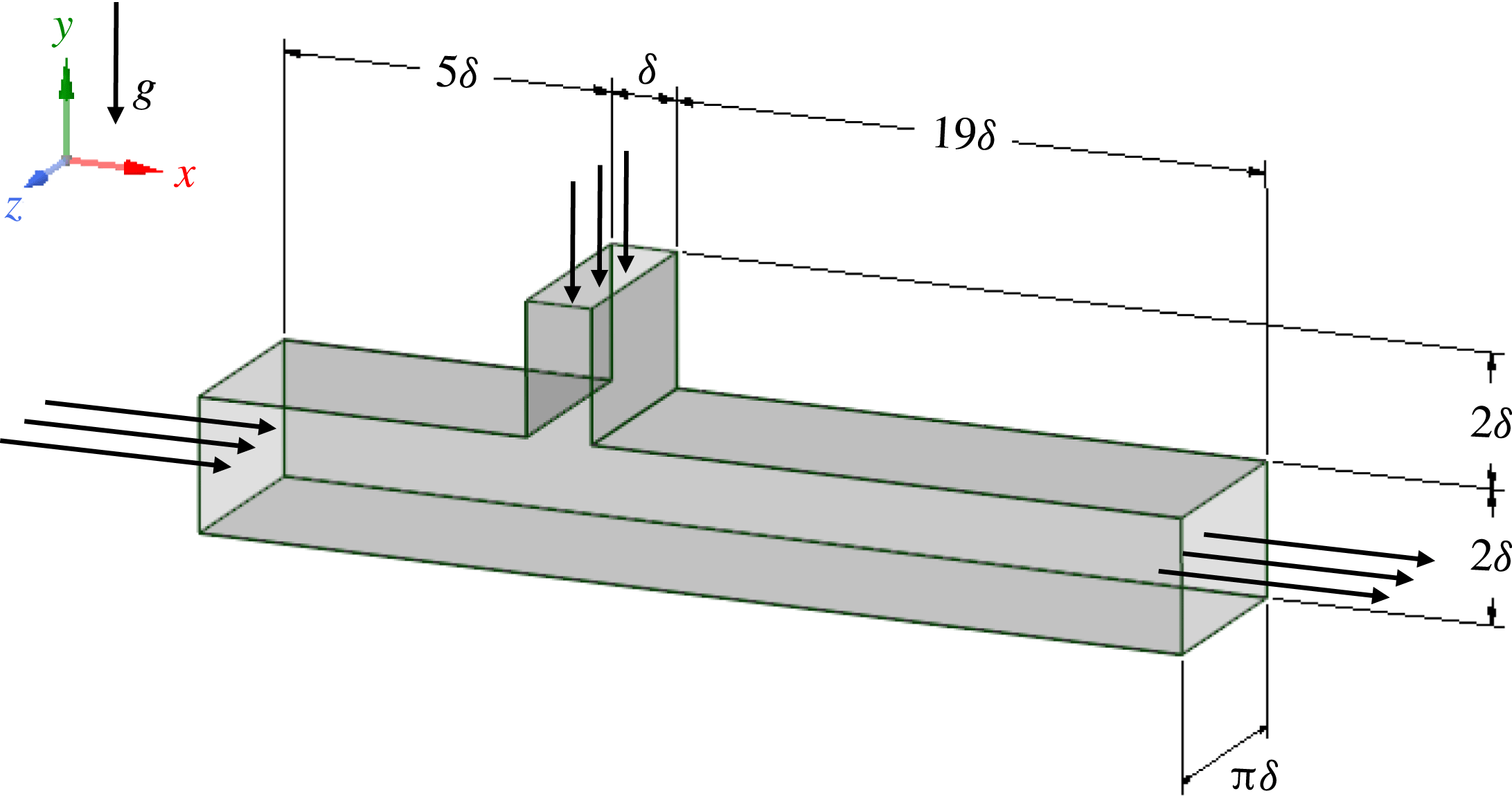
An illustration of the computational domain is shown in figure 1. In determining the extent of the horizontal and vertical channels upstream of the entry of the jet, we have followed the guideline of Muppidi & Mahesh (Reference Muppidi and Mahesh2007). According to this, the distance of an inflow from the T-junction should be at least equal to the width of the corresponding channel, so that the velocity statistics in the vicinity of the T-junction remain unaffected by the inflow. Based on this guideline, the distance between the T-junction and the inflow of the horizontal channel is set to
 $5\unicode[STIX]{x1D6FF}$
, whereas the extent of the vertical channel in the
 $y$
-direction is set to
 $2\unicode[STIX]{x1D6FF}$
. Further, the extent of the horizontal channel downstream of the entry of the jet is set equal to
 $19\unicode[STIX]{x1D6FF}$
so as to capture as far as possible the mixing process between the two streams.
In the spanwise
 $z$
-direction, the incoming jet extends over the entire computational domain, and the flow in this direction is homogeneous. The size of the computational domain in the
 $z$
-direction should be large enough so as to avoid autocorrelation of the flow quantities. On the other hand, it has to be reasonably limited so as to keep the computational cost of the simulations at acceptable levels. For example, in their LES of flows in channels with periodic hills, Fröhlich et al. (Reference Fröhlich, Mellen, Rodi, Temmerman and Leschziner2005) opted for a size of
 $3\unicode[STIX]{x1D6FF}$
. Also, Flores & Jimenez (Reference Flores and Jimenez2010) suggested
 $3\unicode[STIX]{x1D6FF}$
as the minimum spanwise size for channel flow. This suggests that a similar size may be sufficient for the purposes of our study. However, in our case the incoming jet is laminar, which could lead to more persistent two-dimensional structures. For this reason, and in order to gain further insight into the size requirements, we conducted LES with 3 different spanwise sizes,
 $\unicode[STIX]{x03C0}\unicode[STIX]{x1D6FF}$
,
 $(3/2)\unicode[STIX]{x03C0}\unicode[STIX]{x1D6FF}$
and
 $2\unicode[STIX]{x03C0}\unicode[STIX]{x1D6FF}$
, and compared the numerical results. As it turned out, the differences between the first- and second-order statistics of the flow quantities were very small. On the basis of these considerations, the spanwise size of the computational domain in our study is set to
 $\unicode[STIX]{x03C0}\unicode[STIX]{x1D6FF}$
, which is deemed as a satisfactory compromise between required accuracy and computational cost.
Illustration of the computational domain for the T-junction simulation. For visualisation purposes, the drawing is not to scale.

Given these dimensions, the computational grid for the DNS consists of
 $44.16\times 10^{6}$
computational nodes. Due to the significant flow inhomogeneities, in the streamwise and wall-normal directions we have employed non-uniform grid spacing. On the other hand, a uniform grid spacing is used in the homogeneous
 $z$
-direction. Henceforth, all lengths will be given in non-dimensional values, that is, normalised by
 $\unicode[STIX]{x1D6FF}$
. Finally, the origin of the axes is placed at the bottom wall, opposite to the downstream corner of the entry of the jet.
The computational grid can be divided in three sections. The first one covers the horizontal channel upstream of the entry of the jet,
 $-6<x\leqslant -1$
. In this section we have placed 100 computational nodes in the streamwise direction. More specifically, in the zone
 $-6<x\leqslant -2.78$
there are 36 nodes with constant spacing
 $\unicode[STIX]{x0394}x=0.091$
. Then, the grid is progressively refined, with a mild compression ratio of 0.95, up to
 $\unicode[STIX]{x0394}x=0.004$
. The second section is defined by
 $-1<x\leqslant 0$
and includes the vertical channel. Therein we have placed 100 nodes in the streamwise direction with a symmetric distribution with respect to the mid-plane of the vertical channel,
 $x=-0.50$
. For
 $-1<x\leqslant -0.5$
the grid spacing increases smoothly with a stretching factor of 1.03, up to
 $\unicode[STIX]{x0394}x=0.02$
. The third section covers the computational domain downstream of the entry of the jet and is discretised by 900 nodes in the streamwise direction. More specifically, in the interval
 $0<x\leqslant 0.9$
we have placed 85 nodes and the spacing increases with a constant stretching factor of 1.02 up to
 $\unicode[STIX]{x0394}x=0.022$
. Beyond the station
 $x=0.9$
, the streamwise meshing is uniform.
In the wall-normal direction, we have placed 300 cells across the horizontal channel, 140 nodes above and 160 nodes below the mid-plane. The choice of asymmetric meshing in the (wall-normal)
 $y$
-direction is motivated by the fact that in some regions of the bottom wall, the thickness of the boundary layer decreases considerably due to flow acceleration; see figure 7 and the relevant discussion below. Moreover, the fluid at the top wall is colder than the cross-flow and, therefore, has higher shear viscosity. Consequently, the computational requirements at the top wall are not as strict as those at the bottom wall. For these reasons, we opted for higher resolution at the bottom half of the horizontal channel. The centre of the first cell from the bottom wall,
 $y=0$
, is set at
 $y_{f.n.}=8.98\times 10^{-4}$
. In the bottom half of the horizontal channel, the spacing increases smoothly, with a constant stretching factor of 1.013, up to
 $\unicode[STIX]{x0394}y=0.015$
. The remaining 140 nodes are placed at the top half of the channel; therein the grid is refined smoothly as we approach the top wall with a constant stretching factor of 1.012. The first node off the top wall is located at
 $y_{f.n.}=1.33\times 10^{-3}$
. Along the vertical channel,
 $2<y<4$
, we have placed 150 cells. The grid spacing increases smoothly with
 $y$
, with a constant stretching factor of 1.018, up to
 $\unicode[STIX]{x0394}y=0.0195$
at the top inflow boundary.
Finally, in the spanwise direction, the domain is discretised via 128 uniformly distributed nodes, i.e.
 $\unicode[STIX]{x0394}z=0.0245$
. An overview of the discretisation of the computational domain is provided in table 2.
Overview of the discretisation of the computational domain.

In determining the grid spacing in the near-wall regions we have followed the guidelines of Le, Moin & Kim (Reference Le, Moin and Kim1997) according to which at least one node should be placed in the interval
 $0<y^{+}<1$
, while the grid spacing in the streamwise and spanwise directions should be
 $\unicode[STIX]{x0394}x^{+}\approx 10$
and
 $\unicode[STIX]{x0394}z^{+}\approx 15$
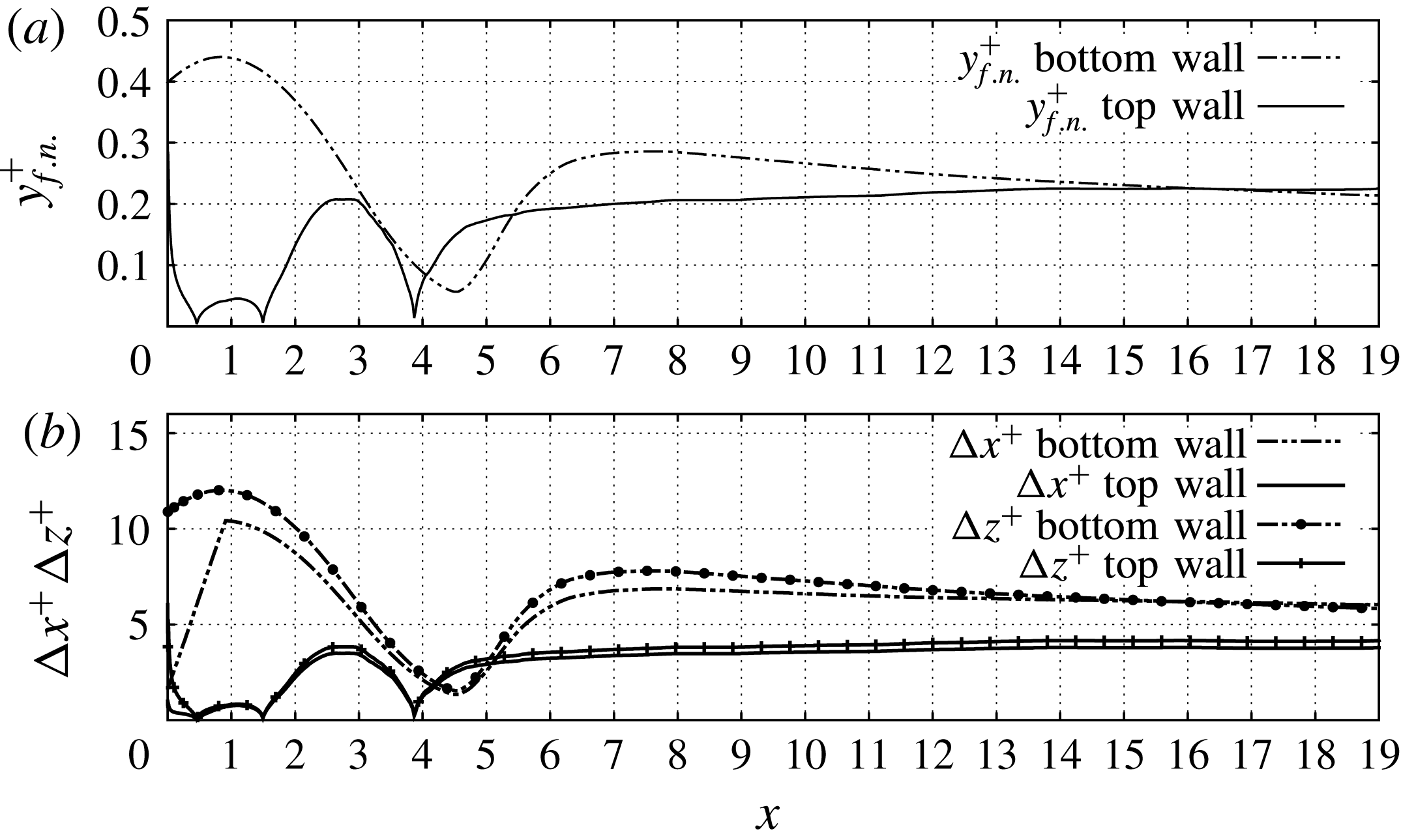
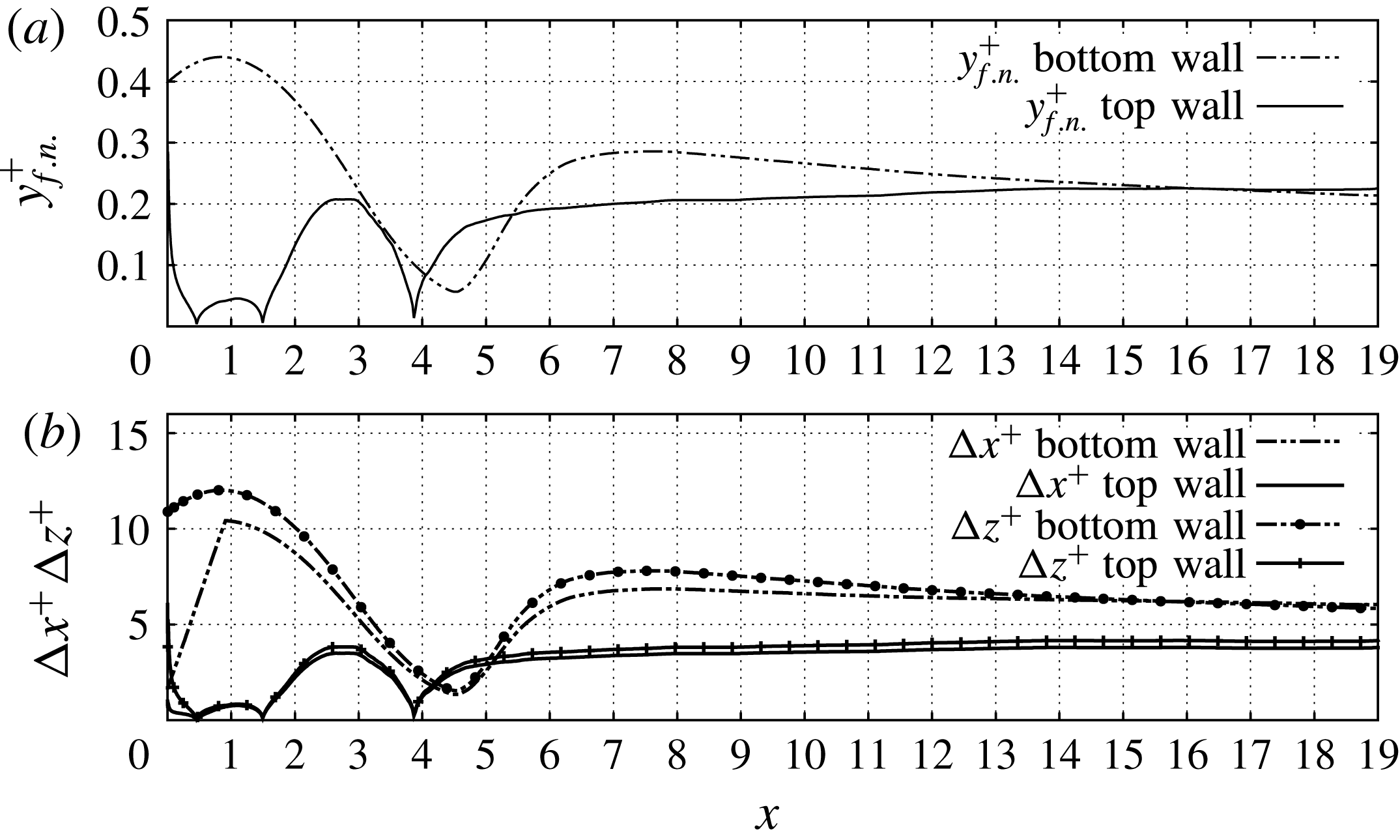
, respectively. In figure 2 we show the position of the first node in the vertical direction and the grid spacing (in wall units) at the walls of the horizontal channel. More specifically, from figure 2(a) we can infer that at least two nodes are always placed in the interval
 $0<y^{+}<1$
. At the bottom boundary,
 $y_{f.n.}^{+}$
attains its maximum value of 0.44 at
 $x\approx 1$
and decreases significantly further downstream. In particular, for
 $x>3.0$
,
 $y_{f.n.}$
becomes smaller than 0.3. At the top boundary,
 $y_{f.n.}^{+}$
is always smaller than 0.3. Further, according to figure 2(b), the coarsest grid spacings at the bottom boundary are
 $\unicode[STIX]{x0394}x^{+}\approx 10.4$
and
 $\unicode[STIX]{x0394}z^{+}\approx 12.0$
, and they occur at the station
 $x=1$
. Further downstream, both grid spacings decrease and are consistently smaller than 8.0. At the top wall, the values of
 $\unicode[STIX]{x0394}x^{+}$
and
 $\unicode[STIX]{x0394}z^{+}$
are even lower and always smaller than 4.0. We therefore conclude that our computational mesh fulfils the above guidelines of Le et al. (Reference Le, Moin and Kim1997) for the near-wall regions.
Grid spacing at the walls of the horizontal channel expressed in wall units. (a)
 $y_{f.n.}^{+}$
, (b)
 $\unicode[STIX]{x0394}x^{+}$
and
 $\unicode[STIX]{x0394}z^{+}$
. At the top wall and at
 $x\approx 0.5$
,
 $x\approx 1.4$
and
 $x\approx 3.9$
, the grid spacing drops to zero because the wall shear stress
 $\unicode[STIX]{x1D70F}_{w}$
vanishes due to reattachment of the flow.
For the assessment of the quality of the grid away from the walls, we compare the local grid spacing,
 $\unicode[STIX]{x0394}=(\unicode[STIX]{x0394}x\,\unicode[STIX]{x0394}y\,\unicode[STIX]{x0394}z)^{1/3}$
with the smallest length scales of the flow, namely, the Kolmogorov scale
 $$\begin{eqnarray}\displaystyle \unicode[STIX]{x1D702}=\left(\frac{\unicode[STIX]{x1D708}^{3}}{\unicode[STIX]{x1D716}_{k}}\right)^{1/4}, & & \displaystyle\end{eqnarray}$$
and the temperature microscale
 $\unicode[STIX]{x1D702}_{\unicode[STIX]{x1D703}}$
. For Prandtl numbers significantly higher than unity,
 $\unicode[STIX]{x1D702}_{\unicode[STIX]{x1D703}}$
is given by the following relationship (Tennekes & Lumley Reference Tennekes and Lumley1972),
 $$\begin{eqnarray}\displaystyle \unicode[STIX]{x1D702}_{\unicode[STIX]{x1D703}}=\unicode[STIX]{x1D702}\left(\frac{1}{Pr}\right)^{1/2}. & & \displaystyle\end{eqnarray}$$
However, in the flow under study, the reference Prandtl number is close to unity;
 $Pr=1.44$
, which corresponds to
 $\unicode[STIX]{x1D702}_{\unicode[STIX]{x1D703}}=0.83\,\unicode[STIX]{x1D702}$
. For this reason, we can examine the quality of the grid on the basis of the Kolmogorov scale
 $\unicode[STIX]{x1D702}$
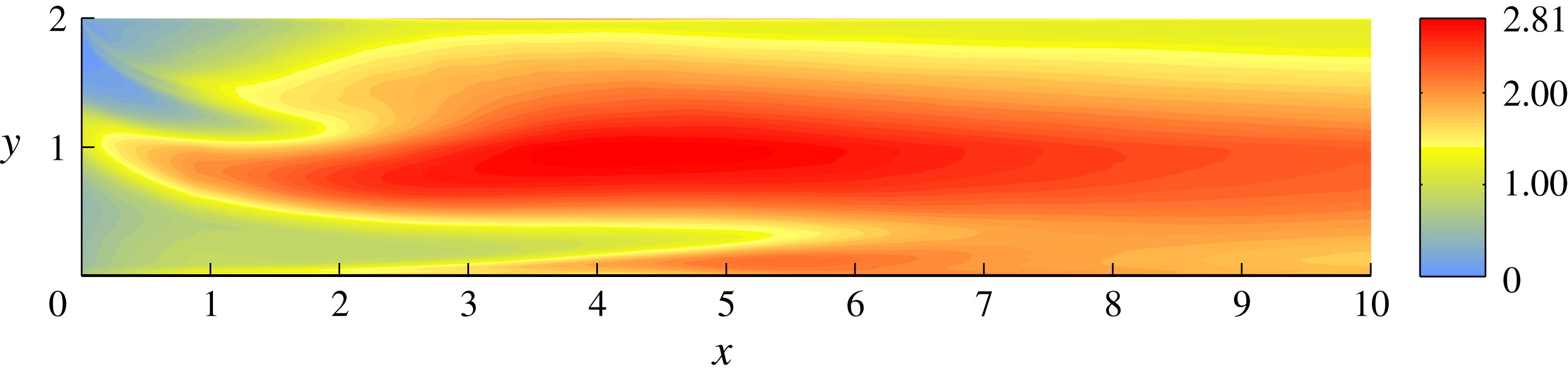
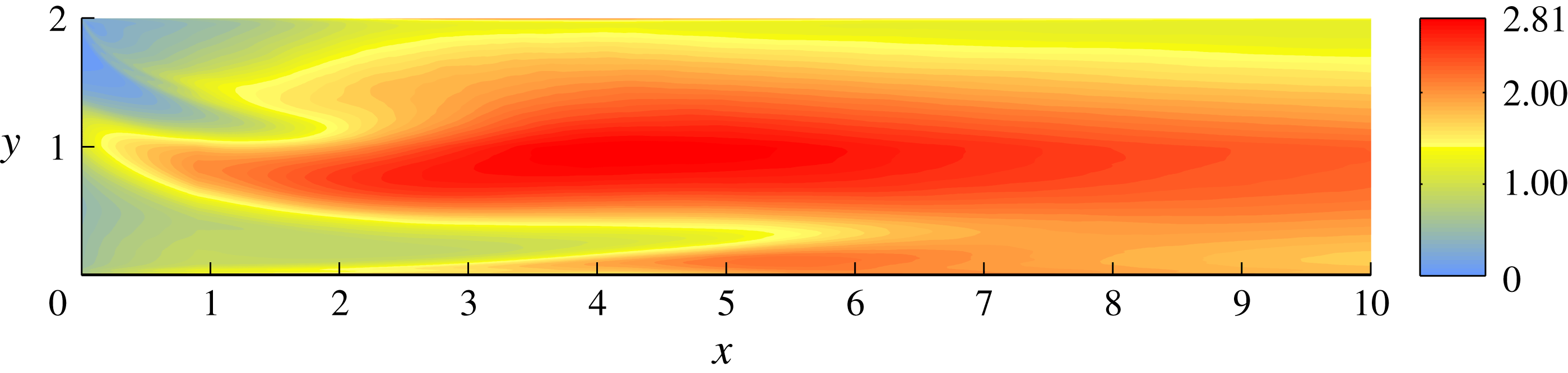
. In figure 3 we present contour plots of the ratio
 $\unicode[STIX]{x0394}/\unicode[STIX]{x1D702}$
downstream of the entry of the jet for the DNS grid. According to this figure, the ratio
 $\unicode[STIX]{x0394}/\unicode[STIX]{x1D702}$
in our grid is close to 2, with a maximum value equal to 2.81. We therefore conclude that our grid resolution for the DNS is sufficient for the purposes of our study.
Finally, for the configuration of the computational mesh of our LES we have followed the guidelines of Zang (Reference Zang1991) so as to fully resolve the wall regions. The stretching factors above and below the entry of the jet are 1.1 and 1.07, respectively. The computational mesh of the LES consists of approximately
 $2\times 10^{6}$
nodes; in other words, it is 22 times coarser than the grid of the DNS. Although the LES mesh resolves the near-wall regions, it does not resolve all turbulent scales away from them; in fact, the ratio
 $\unicode[STIX]{x0394}/\unicode[STIX]{x1D702}$
for the LES mesh is an order of magnitude larger than for the mesh employed in our DNS.
Contour plots of the ratio between the local grid spacing for the DNS and the Kolmogorov length scale,
 $\unicode[STIX]{x0394}/\unicode[STIX]{x1D702}$
, downstream of the entry of the jet.
2.2 Boundary conditions
As regards the implementation of boundary conditions, we have to prescribe a turbulent inflow at the inlet of the cross-flow. In our study, and for purposes of increased accuracy, we produce turbulent inflow data by performing an auxiliary simulation of channel flow simultaneously with the main simulation. In this auxiliary simulation, the streamwise dimension of the computational domain is
 $4\unicode[STIX]{x03C0}\unicode[STIX]{x1D6FF}$
, while the wall-normal and spanwise dimensions are set equal to the ones of the horizontal channel of the T-junction. To avoid spatial interpolation errors, the grid resolution is the same as in the corresponding inlet of the T-junction. The mesh of this auxiliary simulation consists of
 $5.76\times 10^{6}$
computational cells. Also, the same time step is used in the main and auxiliary simulations so as not to introduce time interpolation errors. An analogous procedure is followed for generating turbulent inflow data for the corresponding LES. In particular, we perform an auxiliary wall-resolved LES of channel flow on a grid consisting of
 $4.3\times 10^{5}$
cells. Also, since the incoming jet is laminar, at the top inflow of the vertical channel we impose a parabolic profile whose bulk velocity is equal to unity.
At the outflow boundary, we prescribe a convective boundary condition to all velocity components because it allows the exit of vortical structures from the computational domain with minimal distortion. When applied to a scalar field
 $\unicode[STIX]{x1D719}$
at an outflow plane normal to the
 $x$
-direction, this condition reads
 $$\begin{eqnarray}\displaystyle \frac{\unicode[STIX]{x2202}\unicode[STIX]{x1D719}}{\unicode[STIX]{x2202}t}+U_{conv}\frac{\unicode[STIX]{x2202}\unicode[STIX]{x1D719}}{\unicode[STIX]{x2202}x}=0, & & \displaystyle\end{eqnarray}$$
where the convective velocity
 $U_{conv}$
is set equal to the bulk velocity at the outflow plane.
As regards the temperature field, we prescribe uniform profiles at the two inflows and the convective boundary condition (2.12) at the outflow plane. The walls of the T-junction are considered adiabatic and, therefore, a zero Neumann condition for the temperature is applied at them. Finally, since the flow is homogeneous in the
 $z$
-direction, we prescribe periodic boundary conditions in this direction.
3 Numerical results
This section is devoted to the presentation and analysis of our numerical results. The notation adopted herein is standard; the mean of a generic quantity
 $\unicode[STIX]{x1D719}$
is denoted by
 $\langle \unicode[STIX]{x1D719}\rangle$
and refers to averaging both in time and in the homogeneous spanwise direction. The fluctuating component of
 $\unicode[STIX]{x1D719}$
is denoted by
 $\unicode[STIX]{x1D719}^{\prime }$
, while
 $\unicode[STIX]{x1D719}_{rms}$
stands for the root mean square (r.m.s.) value of
 $\unicode[STIX]{x1D719}^{\prime }$
, i.e.
 $\unicode[STIX]{x1D719}_{rms}=\langle \unicode[STIX]{x1D719}^{\prime }\unicode[STIX]{x1D719}^{\prime }\rangle ^{1/2}$
.
The simulations are initialised by injecting the cold fluid from the vertical channel to the hot cross-flow. The accumulation of data for the statistical analysis of the flow field starts once the flow becomes statistically stationary. To ensure flow stationarity, we first let the simulation run for 8 ‘flow-through’ times. A flow-through time is approximated by the ratio between the length of the horizontal channel past the incoming jet and the bulk velocity of the flow just downstream of the recirculation bubble, i.e. it is approximately equal to
 $19/1.5=12.67$
time units. After 8 flow-through times we start collecting statistics. Flow stationarity is then verified by comparing statistics with an increasing number of samples (and hence increasing flow time over which statistics are computed). Once statistical stationarity is verified, we compute statistics of the flow quantities over 55 time units.
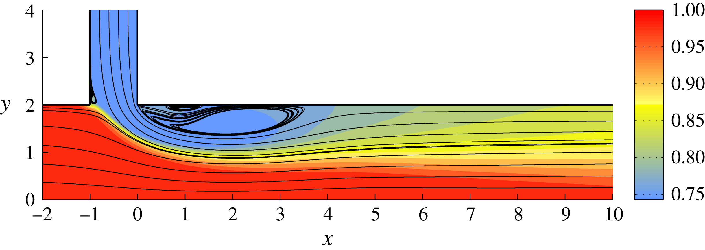
In figure 4 we present streamlines extracted from the mean velocity field superposed by contour plots of the mean temperature
 $\langle T\rangle$
, as computed by the DNS. The basic features of the flow field are similar to the ones of gas–gas flows in T-junctions (Georgiou & Papalexandris Reference Georgiou and Papalexandris2017b
). More specifically, the cross-flow tilts downwards due to the incoming jet. Reciprocally, the jet bends and eventually aligns with the cross-flow. The bending of the jet leads to the formation of a large recirculation bubble near the top wall. In turn, the presence of the bubble decreases the cross-section areas of the cross-flow and the incoming jet. Consequently, the two streams are subject to a Venturi effect and, therefore, accelerate. Then, the two streams expand as they pass by the recirculation bubble, which results in an adverse pressure gradient in the region defined by
 $2<x<6$
. This region includes the reattachment point at the end of the large recirculation bubble, located at
 $x\approx 3.89$
.
Streamlines extracted from the mean velocity field, superposed by contour plots of the mean temperature field
 $\langle T\rangle$
as computed from the DNS.
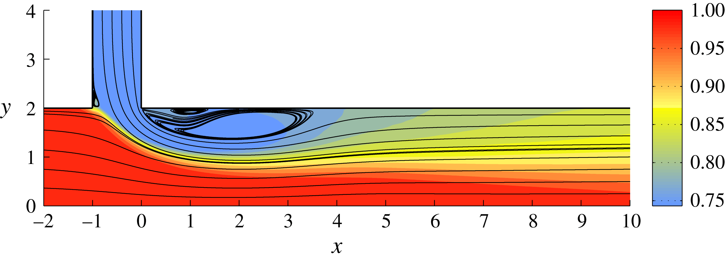
Additionally, figure 4 serves to identify the two shear layers that are developed in the flow field. The first one is formed between the cross-flow and the incoming jet and originates in the vicinity of the upstream corner of the entry of the jet. Henceforth, it will be referred to as the primary shear layer. The second one is formed between the jet and the recirculation bubble, and it will be referred to as the secondary shear layer. These two layers spread rapidly and start to interact, eventually merging to a single shear layer.
Further, in figure 4 we can distinguish two secondary recirculation zones. The first one is located between the downstream corner of the entry of the jet and the large recirculation bubble. A similar structure was identified previously in our LES of gas–gas flow in T-junctions (Georgiou & Papalexandris Reference Georgiou and Papalexandris2017a ,Reference Georgiou and Papalexandris b ). The second one is located inside the vertical channel and close to the upstream corner of the entry of the jet.
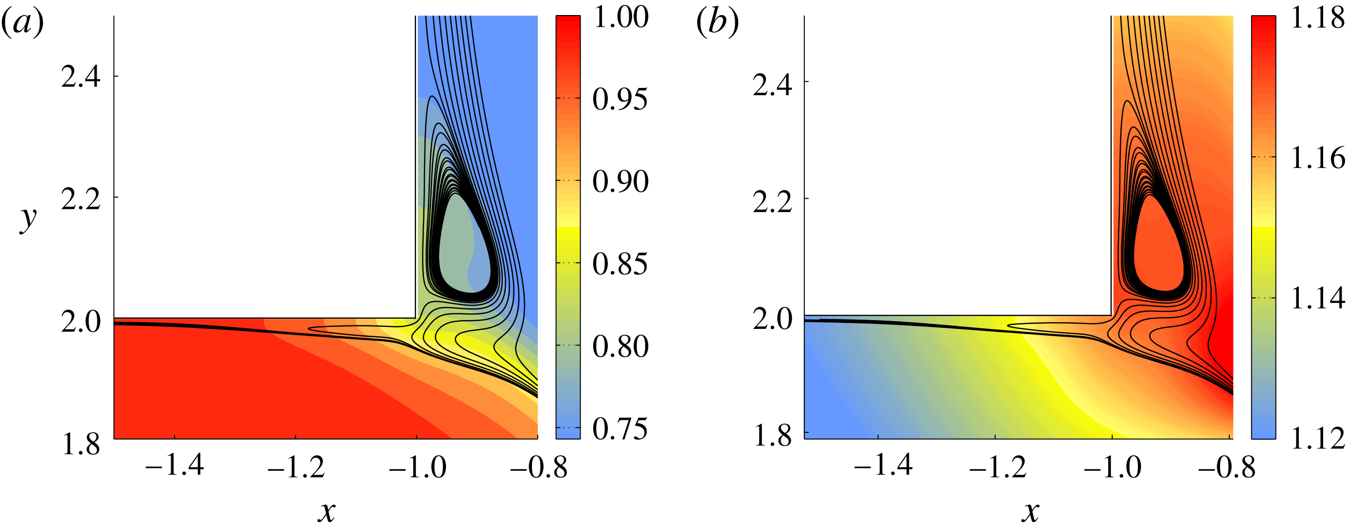
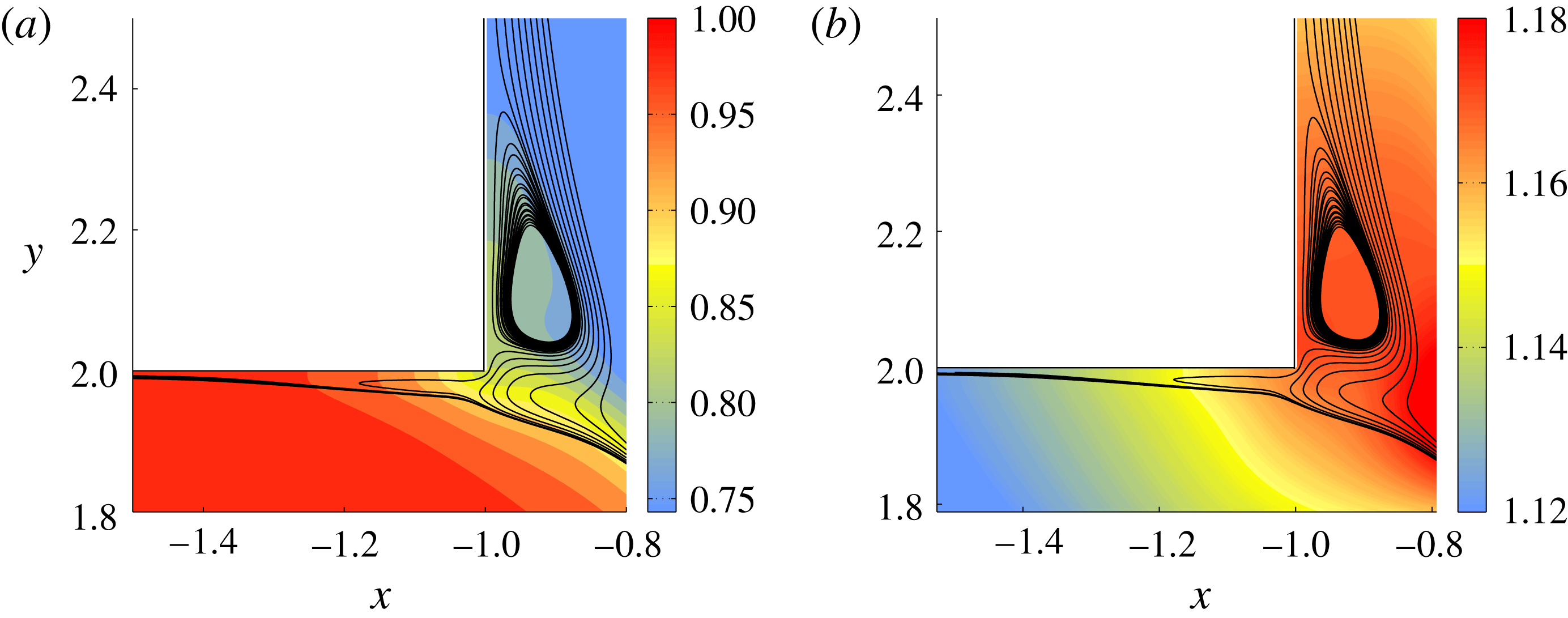
In figures 5(a) and 5(b) we provide a close-up view of the streamlines in the vicinity of the upstream corner, superposed by contour plots of the mean temperature
 $\langle T\rangle$
and pressure
 $\langle p\rangle$
, respectively. We can observe that the recirculation zone inside the vertical channel consists of fluid coming from the incoming jet. In other words, this zone results from the separation of the flow in the vertical channel. As explained in Georgiou & Papalexandris (Reference Georgiou and Papalexandris2017b
), this occurs when the boundary layer at the vertical wall is laminar or when the momentum ratio between the two streams is sufficiently high. In the flow under study, the momentum ratio is quite low,
 $M_{R}=1.89$
. Therefore, the separation of the flow inside the vertical channel is attributed to the laminarity of the boundary layer. Moreover, we can readily observe that in the vicinity of this corner, a small portion of the jet reverses direction and turns upstream. This feature, which has not been observed in previous studies of flows in T-junctions, is due to the combination of low momentum ratio and flow separation inside the vertical channel.
Secondary recirculation zones near the upstream corner of the entry of the jet. This figure shows streamlines extracted from the mean velocity field superposed by contour plots of (a) the mean temperature
 $\langle T\rangle$
, and (b) the mean pressure
 $\langle p\rangle$
. The flow inside the vertical channel separates and forms a small recirculating zone. Also, at this corner the jet reverses direction and bends upstream.
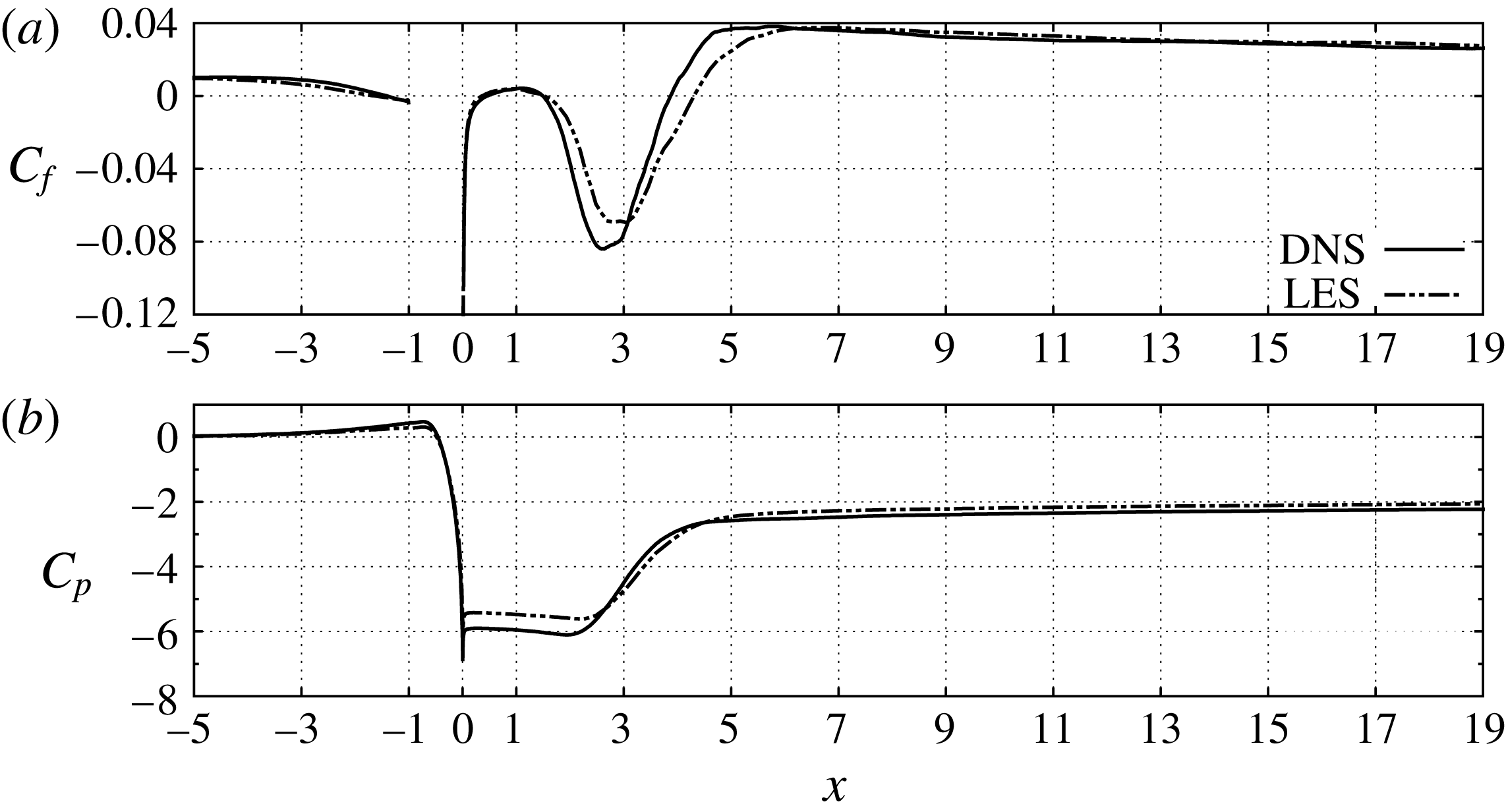
In order to gain insight of the flow properties at the near-wall regions, we examine the variation of the skin friction and pressure coefficients,
 $$\begin{eqnarray}\displaystyle C_{f}=\frac{\langle \unicode[STIX]{x1D70F}_{w}\rangle }{\frac{1}{2}\unicode[STIX]{x1D70C}_{ref}\,U_{ref}^{2}}\quad \text{and}\quad C_{p}=\frac{\langle p\rangle -p_{ref}}{\frac{1}{2}\unicode[STIX]{x1D70C}_{ref}\,U_{ref}^{2}}, & & \displaystyle\end{eqnarray}$$
respectively, along the walls of the horizontal channel. In the above expression,
 $p_{ref}$
and
 $\unicode[STIX]{x1D70C}_{ref}$
are the static pressure and density at the inlet of the cross-flow. The profiles of
 $C_{f}$
and
 $C_{p}$
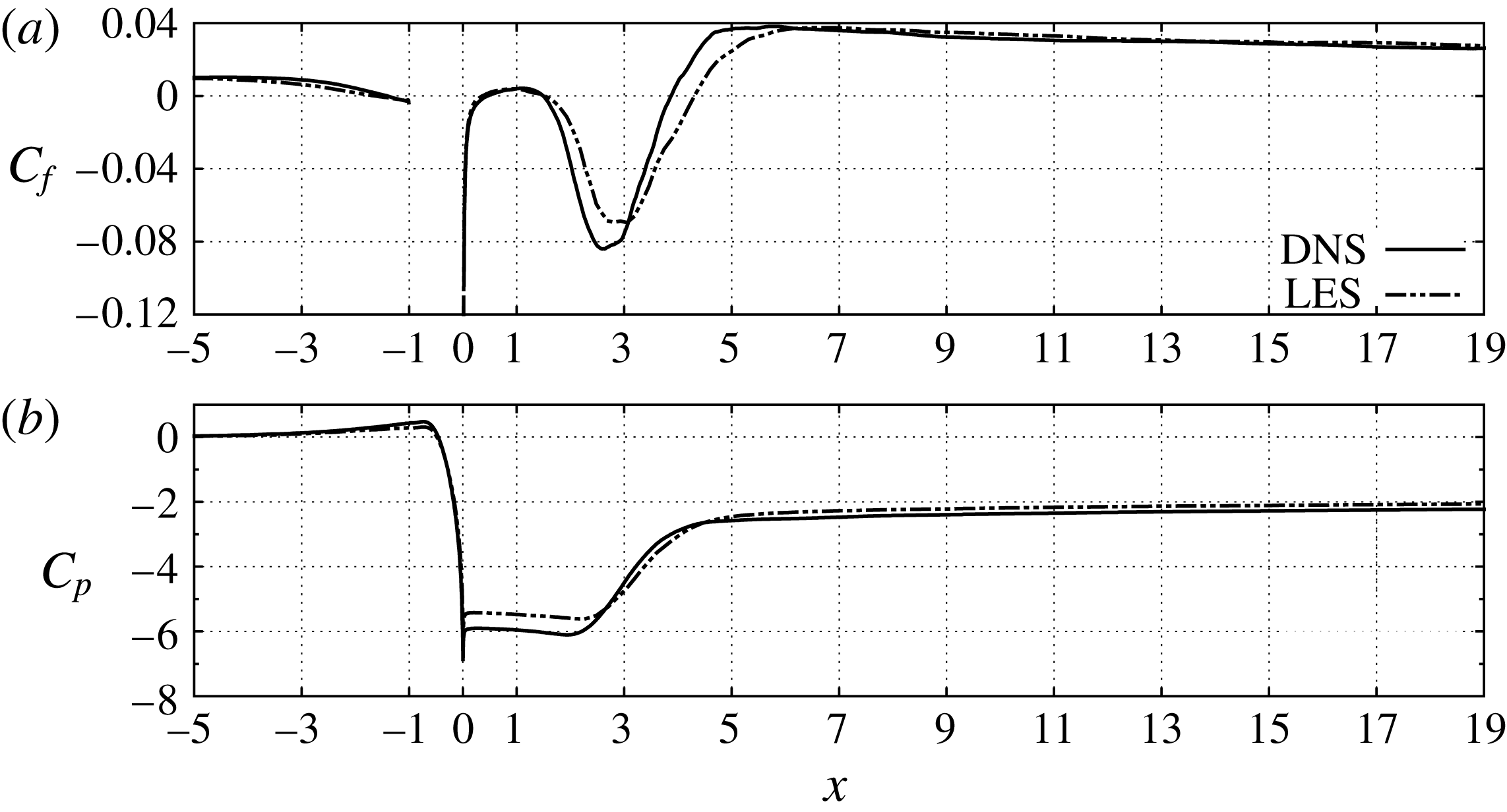
at the top wall, as predicted by the DNS and the LES, are plotted in figure 6. As the cross-flow approaches the entry of the jet, the pressure coefficient
 $C_{p}$
increases, i.e. the pressure increases in the streamwise direction, while
 $C_{f}$
decreases and becomes negative close to the upstream corner. This is due to the reversal of the jet in the vicinity of the upstream corner that was mentioned above. Also, the large drop in
 $C_{p}$
that is observed in the zone
 $-0.5<x<0$
is due to the acceleration of the jet upon its entry in the horizontal channel, i.e. it is due to the aforementioned Venturi effect. Downstream of the entry of the jet, at the large recirculation bubble,
 $C_{f}$
decreases considerably and attains large negative values, whereas
 $C_{p}$
is kept almost constant. However, as we approach the reattachment point of the flow, both coefficients increase. This is a manifestation of the adverse pressure gradient that is formed as the two streams expand. Further downstream and up to the outflow boundary, the values of
 $C_{f}$
remain higher than at the inlet of the cross-flow. This is attributed, primarily, to the thinning of the boundary layer due to the acceleration of the flow (the incoming jet increases the flow rate across the channel by approximately 50 %) and, secondarily, to the increased shear viscosity resulting from the lower temperatures near the top wall.
Plots of the skin friction and pressure coefficients,
 $C_{f}$
and
 $C_{p}$
, at the top wall of the horizontal channel. (a)
 $C_{f}$
, (b)
 $C_{p}$
. The interval
 $-1<x<0$
corresponds to the entry of the jet and, therefore,
 $C_{f}$
is not defined therein.
Plots of the skin friction and pressure coefficients,
 $C_{f}$
and
 $C_{p}$
, at the bottom wall of the horizontal channel. (a)
 $C_{f}$
, (b)
 $C_{p}$
.
As concerns the comparison between the two simulations, the predictions of the LES agree well with those of the DNS for both
 $C_{f}$
and
 $C_{p}$
. However, the LES produces a slightly diffused profile of
 $C_{f}$
in the region of the recirculation bubble. Further, the LES predicts slightly higher values of
 $C_{p}$
in the vicinity the downstream corner of the entry of the jet.
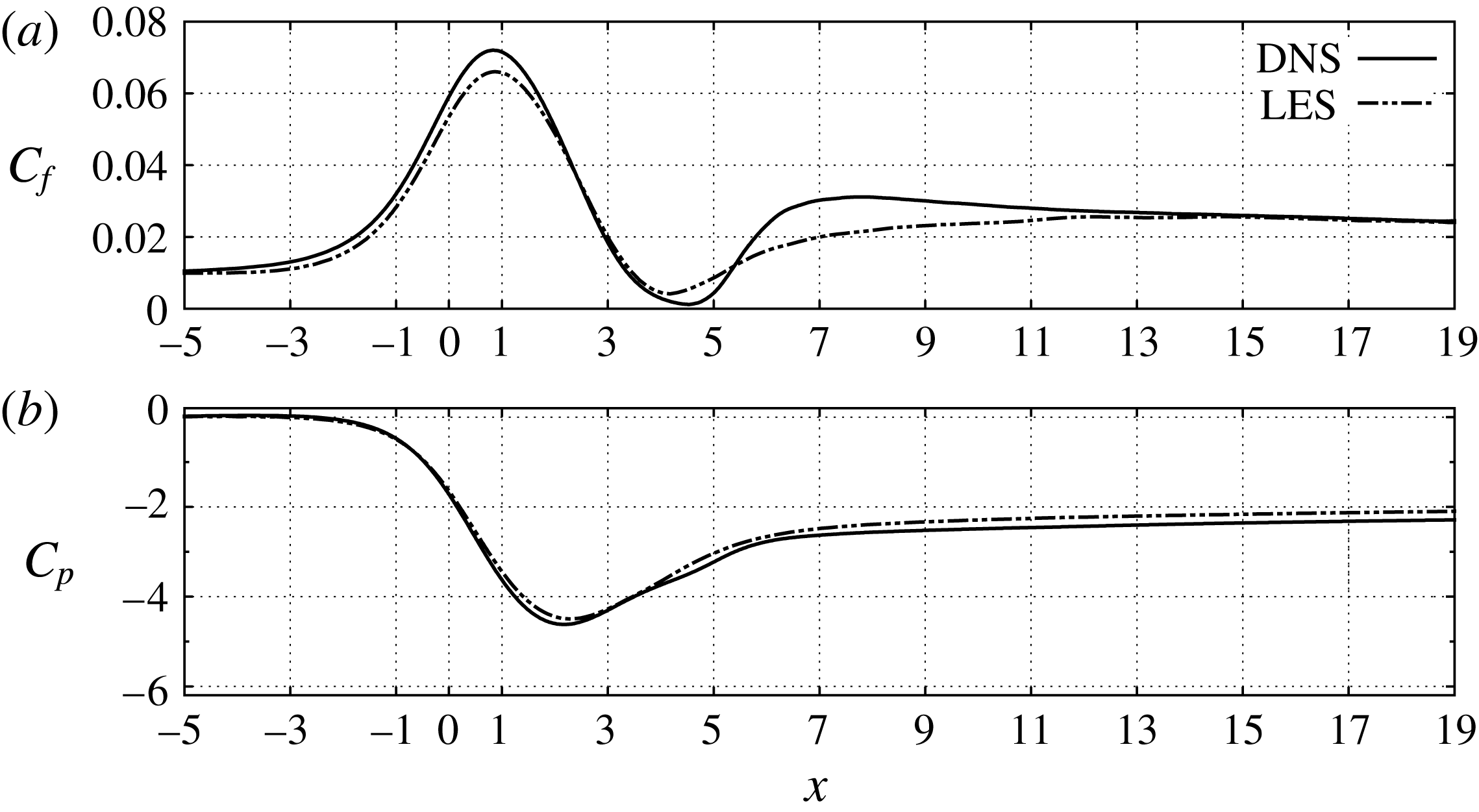
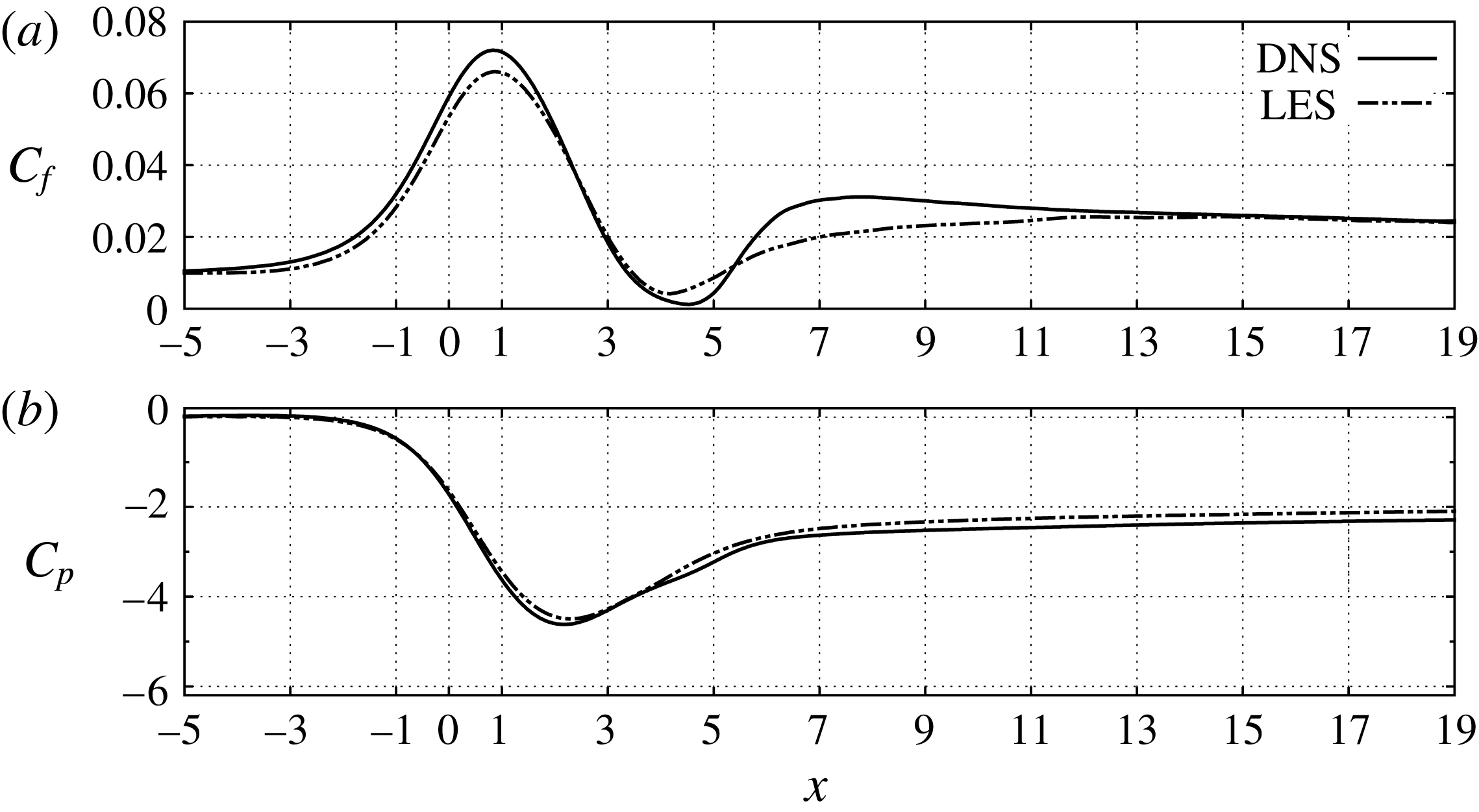
In figure 7 we present the plots of
 $C_{f}$
and
 $C_{p}$
along the bottom wall. In the interval
 $-1<x<1$
these coefficients follow opposite trends as the former increases while the latter decreases. This is a consequence of the acceleration of the cross-flow due to the Venturi effect, which produces a strong favourable pressure gradient and increases the shear stress
 $\unicode[STIX]{x1D70F}_{w}$
at the bottom wall. Further, the acceleration and streamlining of the cross-flow result in the thinning of the boundary layer and the decrease of the local turbulent intensity, as can be verified by the mean and r.m.s. velocity profiles shown in § 3.2. These are typical characteristics of local flow relaminarisation, or reverse transition, in accelerated turbulent boundary layers (Sreenivasan Reference Sreenivasan1982). For more information on this topic, the reader is referred to the recent work of Bourassa & Thomas (Reference Bourassa and Thomas2009) and to references therein.
Nonetheless, the flow relaminarisation is fairly localised. In fact, in the region
 $2<x<5$
the cross-flow expands, leading to the formation of the adverse pressure gradient mentioned above. Also in this region, the flow has a tendency to separate but
 $C_{f}$
remains positive across the bottom wall. Finally, as regards the comparison between the two simulations, the LES and DENS results for
 $C_{p}$
are almost identical. Also, the results for
 $C_{f}$
agree fairly well, albeit the LES profile is somewhat diffused in the zone of the expansion of the cross-flow.
3.1 Instantaneous flow structures
In this subsection we examine the instantaneous flow structures, as extracted from the DNS data. In our analysis we focus on the primary and secondary shear layers and assess their contribution to the mixing process in the T-junction. We also investigate the effect of the incoming jet on the flow structures near the top and bottom walls. All the figures presented herein show results at the same time instance.
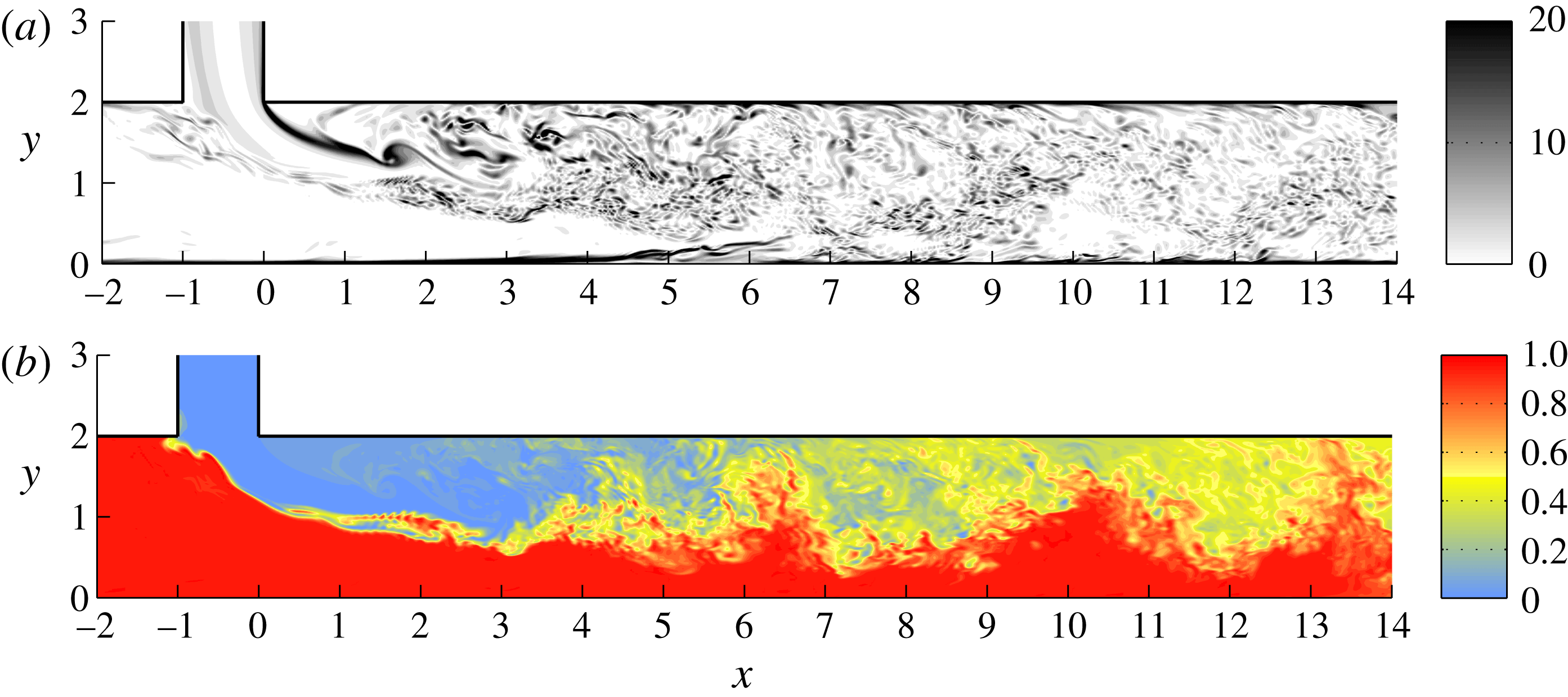
In figure 8 we provide contour plots of the amplitude of the instantaneous spanwise vorticity
 $|\unicode[STIX]{x1D714}_{z}|$
and normalised temperature
 $\unicode[STIX]{x1D703}$
,
 $$\begin{eqnarray}\displaystyle \unicode[STIX]{x1D703}=\frac{T-T_{jet}}{T_{ref}-T_{jet}}. & & \displaystyle\end{eqnarray}$$
The results shown in this figure are taken at the
 $xy$
-plane defined by
 $z=1.24$
.
Contour plots of the amplitude of the instantaneous spanwise vorticity
 $|\unicode[STIX]{x1D714}_{z}|$
and normalised temperature
 $\unicode[STIX]{x1D703}$
at
 $z=1.24$
. (a)
 $|\unicode[STIX]{x1D714}_{z}|$
, (b)
 $\unicode[STIX]{x1D703}$
. In (a) we observe the formation of a large spanwise roller at the secondary shear layer at
 $x\approx 1.8$
.
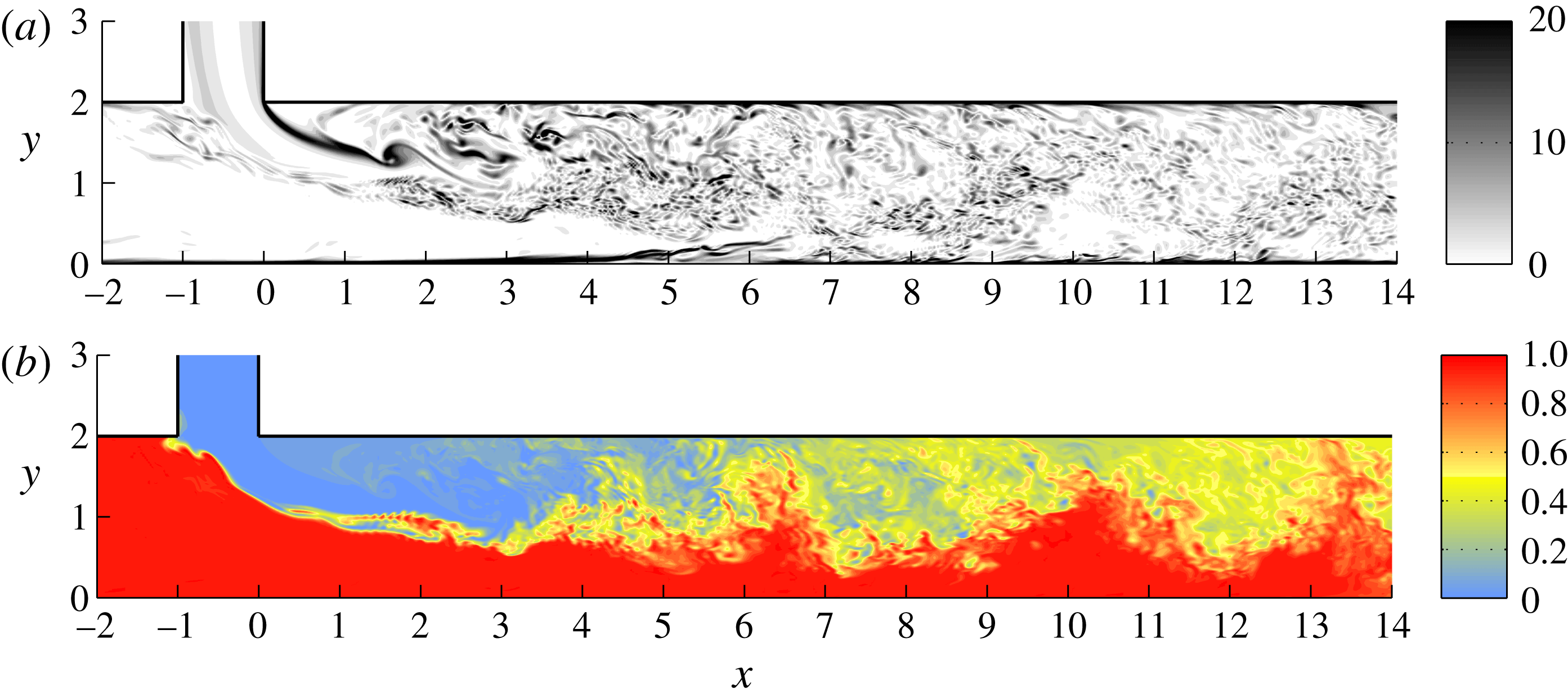
Both shear layers roll up quickly, leading to the formation and shedding of spanwise rollers such as the one spotted at the secondary layer and at
 $x\approx 1.8$
, see figure 8(a). These rollers merge with adjacent ones in a pairing process, or they are torn apart and their vorticity is absorbed by the surrounding vortical structures. Most of the surviving rollers are convected downstream but some of them interact with the large recirculation bubble and eventually get entrapped therein. Also, as the two shear layers spread, they start to interact and, eventually, merge. Downstream of the reattachment point of the flow, the merged shear layer continues to spread until it extends across the entire channel. In fact, downstream of the station
 $x=6.0$
, many of its rollers interact with the bottom wall. Additionally, we can observe numerous thin and elongated vortical structures close to the bottom wall for
 $4<x<7$
. Their formation is attributed to the deceleration of the flow caused by the adverse pressure gradient in this region, see figure 7(b).
In regard to the instantaneous temperature field, shown in figure 8(b), we remark that thermal mixing is initiated by the spanwise rollers of the primary shear layer close to the upstream corner of the entry of the jet. The mixing process is significantly enhanced once the two shear layers start to interact with one another. Also, downstream of the large recirculation bubble, we can observe the effect of the surviving rollers as they transport hot fluid originating from the cross-flow toward the top wall. A video animation of the evolution of the temperature field in the
 $(xy)$
plane is provided as supplementary movie 1 (available at https://doi.org/10.1017/jfm.2018.256).
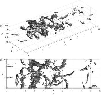
In figure 9 we show isosurface plots of the fluctuating pressure at the value
 $p^{\prime }=-0.25$
. Such plots are frequently used for the identification of large coherent structures. In our case, the value
 $p^{\prime }=-0.25$
has been chosen because it provides a clear visualisation of these structures. The growth of the spanwise rollers from the secondary shear layer can be inferred from the three-dimensional view of figure 9(a). These rollers are convected downstream and eventually are torn apart into smaller structures in a highly turbulent environment. Also, from figure 9(b) which shows a projection of the isosurface plot of
 $p^{\prime }$
at the
 $xz$
-plane, we can observe the formation of streamwise vortex tubes, known as ‘rib’ vortices, that connect two adjacent spanwise rollers. On the other hand, the smaller streamwise vortex tubes close to the upstream corner of the entry of the jet,
 $x=0.0$
, are part of the primary shear layer and eventually break up into smaller ones.
Isosurface plots of the fluctuating pressure at the value
 $p^{\prime }=-0.25$
. (a) Three-dimensional view, (b) view from above (
 $xz$
-plane). The large spanwise rollers shown in these plots are shed by the secondary shear layer. Also, the streamwise vortex tubes connecting two consecutive rollers correspond to ‘rib’ vortices.

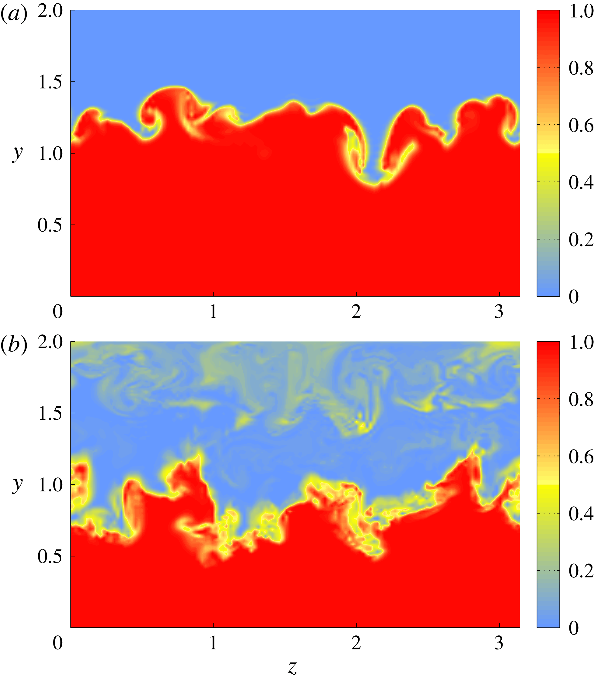
In order to elucidate the role of these streamwise vortex tubes to the mixing process, in figure 10 we present contour plots of
 $\unicode[STIX]{x1D703}$
at two streamwise stations, namely, at
 $x=0.0$
and
 $x=3.0$
. At the first station, these tubes are located at the primary shear layer and are part of mushroom-like structures that are formed right at the interface of the two streams. A mushroom moving upwards is formed by fluid coming from the cross-flow and wraps around itself cold fluid from the incoming jet, thus forming a spiral (Lin & Corcos Reference Lin and Corcos1984). Inversely, a mushroom moving downwards is formed by fluid coming from the jet and wraps around itself hot fluid from the cross-flow. Such mushroom-like structures are typical of turbulent mixing layers (Corcos & Lin Reference Corcos and Lin1984; Bernal & Roshko Reference Bernal and Roshko1986; Rogers & Moser Reference Rogers and Moser1992) and have also been observed experimentally in the shear layers of T-junctions (Hirota et al.
Reference Hirota, Mohri, Asano and Goto2010). A video animation of the evolution of the temperature field at this streamwise station is provided as supplementary movie 2. At the second station,
 $x=3.0$
, the primary and secondary shear layers have started to interact and these mushroom-like structures have already broken up. Instead, the vorticity field therein is dominated by the large spanwise rollers of the secondary shear layer.
Contour plots of the instantaneous normalised temperature
 $\unicode[STIX]{x1D703}$
at two streamwise locations. (a)
 $x=0.0$
, (b)
 $x=3.0$
. In (a) we can observe the formation of mushroom-like structures of streamwise vorticity at the primary shear layer. However at
 $x=3.0$
, (b) these structures have already been broken up.

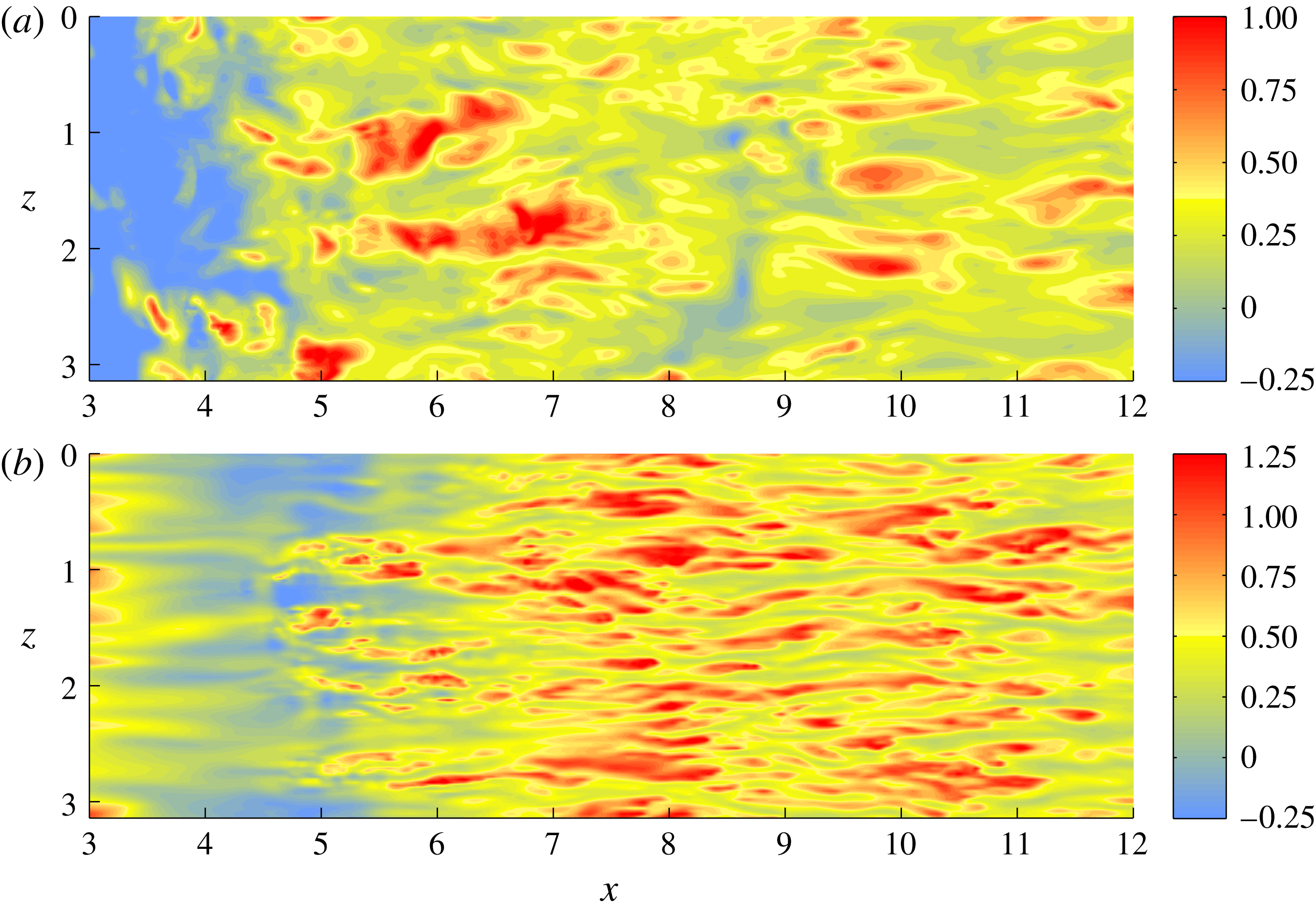
Our analysis of the instantaneous flow structures concludes with the examination of the near-wall regions. In figure 11 we present contour plots of the instantaneous streamwise velocity
 $u$
close to the walls of the horizontal channel. In the vicinity of the reattachment point of the flow, vortical structures emanating from the shear layers interact with the top wall, leading to the formation of several irregularly shaped streaks. On the other hand, further downstream, the adverse pressure gradient results in the widening and weakening of the velocity streaks. This feature is typical of regions of adverse pressure gradient; see, for example the discussion in Skote & Henningson (Reference Skote and Henningson2002) and Lee et al. (Reference Lee, Hu, Saha and Kazimi2009). At the bottom wall and in the region
 $4<x<5$
, there are patches of negative streamwise velocity. This is also due to the adverse pressure gradient which causes the flow to decelerate. It should be noted, however, that this concerns instantaneous values, whereas the mean streamwise velocities remain positive close to the bottom wall. Also, further downstream, we identify zones with numerous velocity streaks. These streaks are much longer and thinner than the ones observed near the top wall and are caused by the interaction of vortices from the merged shear layer with the bottom wall.
Contour plots of the instantaneous streamwise velocity
 $u$
close to the two walls of the horizontal channel. (a) Top wall,
 $y=1.98$
, (b) bottom wall,
 $y=0.02$
.

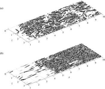
Finally, in figure 12 we show a representation of the instantaneous vorticity field at the walls, based on the quantity
 $Q$
. This quantity, introduced by Hunt, Wray & Moin (Reference Hunt, Wray and Moin1988), measures the difference between the amplitudes of the symmetric and skew-symmetric parts of the velocity-gradient tensor, and it aids the visualisation of the vorticity field. In particular, positive values of
 $Q$
correspond to non-zero vorticity amplitude. Also, the higher the value of
 $Q$
is, the higher the vorticity amplitude gets. In figure 12 we present plots of the isosurface of the value
 $Q=4.0$
. At the top wall, we can observe numerous irregularly oriented vortical structures in the region covered by the large recirculation bubble. Downstream of the reattachment of the flow, the density of these structures gradually decreases. The dense patches of interwoven vorticity that can be observed in this region coincide with the widened velocity streaks observed in figure 11(a).
According to figure 12(b), near the bottom wall there are very few vortical structures for
 $x<4$
. This is the region where the cross-flow accelerates due to the Venturi effect. Downstream of this region, we observe a large number of vortical structures. Some of them are formed due to the adverse pressure gradient caused by the expansion of the cross-flow, while others are transported by the merged shear layer which spreads and interacts with the bottom wall. We also remark that, for
 $x>4$
, the density of the vortical structures at the bottom wall is higher than at the top wall. This difference may be attributed to two factors. The first one is that the local velocity close to bottom top wall is more than twice the local velocity close to the top one. The second factor is the lower temperature and, therefore, higher viscosity of the fluid at the top which enhances dissipation of the vortical structures.
Isosurface plots of the
 $Q$
-criterion (
 $Q=4.0$
) at the wall regions. (a) Top wall, (b) bottom wall.

3.2 Flow statistics
We first present the first- and second-order statistics of the temperature field and also compare the LES predictions with the DNS data. Figure 13 shows the profiles of the averaged normalised temperature
 $\langle \unicode[STIX]{x1D703}\rangle$
at different streamwise stations. The main feature of these profiles is the transition zone from the high temperature at the bottom to the low temperature at the top. Close to the entry of the jet, this transition takes place across the primary shear layer. Also, at the stations
 $x=1.0$
and
 $x=3.0$
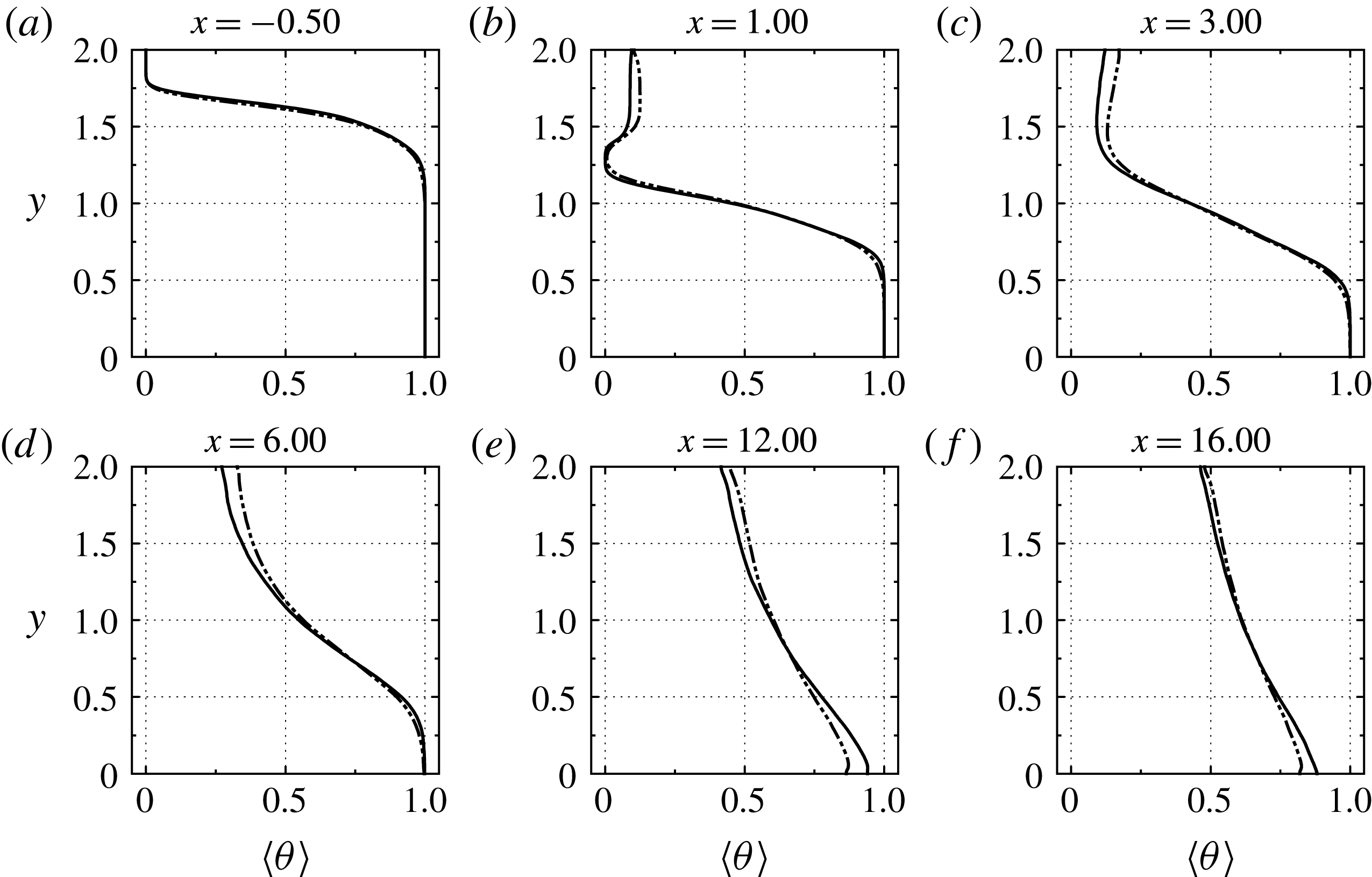
, i.e. at the large recirculation bubble, the temperature profile is not monotonic but attains a minimum at the core of the secondary shear layer. In other words, the temperature in the recirculation bubble is higher than in the secondary layer. This implies that the bubble does not consist solely of fluid from the incoming jet but it also contains fluid from the hot cross-flow.
Further downstream, the two shear layers merge and a monotonic temperature profile is established due to thermal mixing. As the flow evolves and thermal mixing progresses, the temperature gradients become weaker. Also, the temperature profile becomes essentially linear, as can be asserted from figure 13(f). Since the solid walls are adiabatically isolated, a channel flow of uniform temperature will eventually emerge; however, thermal equilibrium is not established within the limits of our computational domain.
Profiles of the mean normalised temperature
 $\langle \unicode[STIX]{x1D703}\rangle$
at different streamwise stations of the horizontal channel. ——, DNS; — ⋅ ⋅ —, LES.

We also remark that the LES predictions agree well with the DNS data and their differences are minor. For example, the LES slightly overpredicts the temperature inside the recirculation bubble, while further downstream at (
 $x=12.0$
and
 $x=16.0$
) there is a small discrepancy in the prediction of the temperature at the bottom wall.
The profiles of the r.m.s. normalised temperature
 $\unicode[STIX]{x1D703}_{rms}$
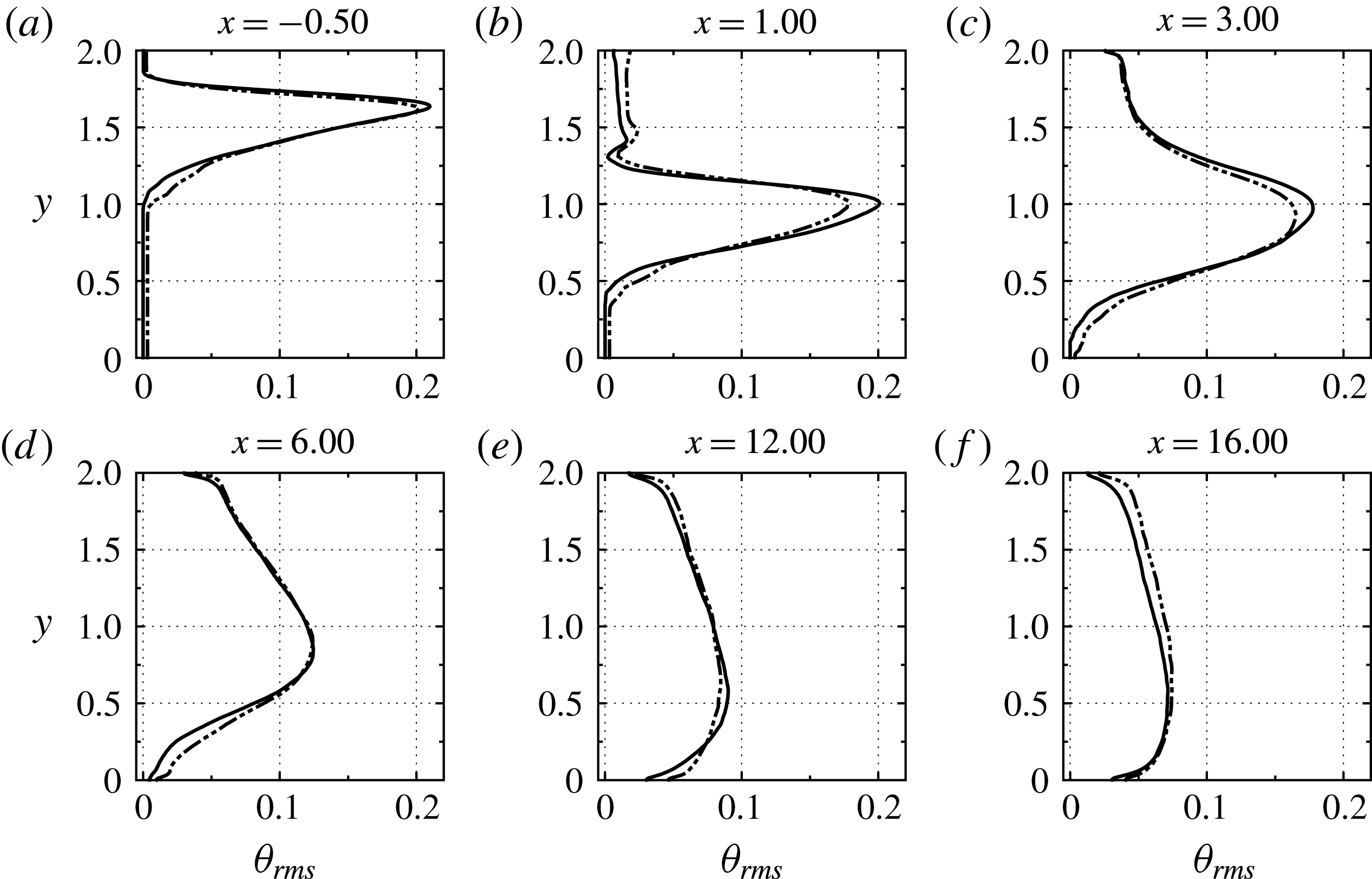
are shown in figure 14. Their most characteristic feature is the peak due to the primary shear layer. At
 $x=1.0$
this peak is very sharp. However, as the shear layer spreads out, the value of the peak drops and its location moves closer to the bottom wall. In turn, this implies that thermal mixing is most intense in the region between
 $x=0.0$
and
 $x=4.0$
. In this figure we also observe that the predictions of the LES agree very well with those of the DNS, albeit the LES mildly underpredicts the amplitudes of the peaks of
 $\unicode[STIX]{x1D703}_{rms}$
at
 $x=1.0$
and
 $x=3.0$
.
Profiles of the r.m.s. of the normalised temperature
 $\unicode[STIX]{x1D703}_{rms}$
at different streamwise stations of the horizontal channel. ——, DNS; — ⋅ ⋅ —, LES.

We proceed with the presentation of the velocity statistics. The profiles of the mean streamwise velocity
 $\langle u\rangle$
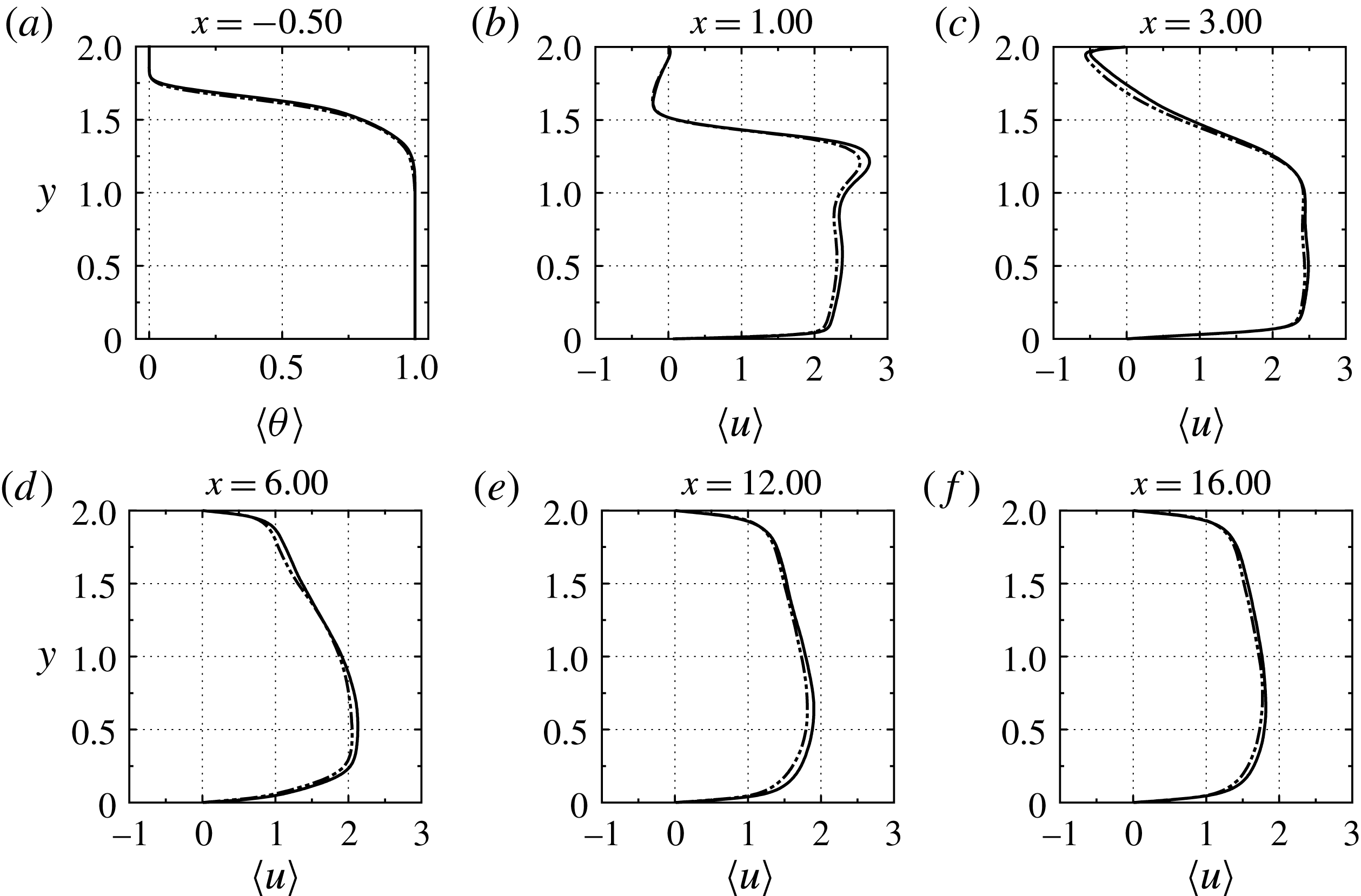
are shown in figure 15. The negative values at the top wall for
 $x=1.0$
and
 $x=3.0$
occur inside the recirculation bubble. Also, the high wall-normal gradients of
 $\langle u\rangle$
at these streamwise stations correspond to the secondary shear layer. Downstream of the reattachment of the flow, the mean velocity converges to a channel-flow profile, albeit at a slow rate as can be attested by the asymmetry of the profiles shown in figure 15(d–f). We also remark that the LES predictions of
 $\langle u\rangle$
compare quite favourably with the DNS data at all streamwise stations.
Profiles of the mean streamwise velocity
 $\langle u\rangle$
at different streamwise stations of the horizontal channel. ——, DNS; — ⋅ ⋅ —, LES.

In figure 16 we present plots of the r.m.s. profile of the streamwise velocity,
 $u_{rms}$
. The maximum at
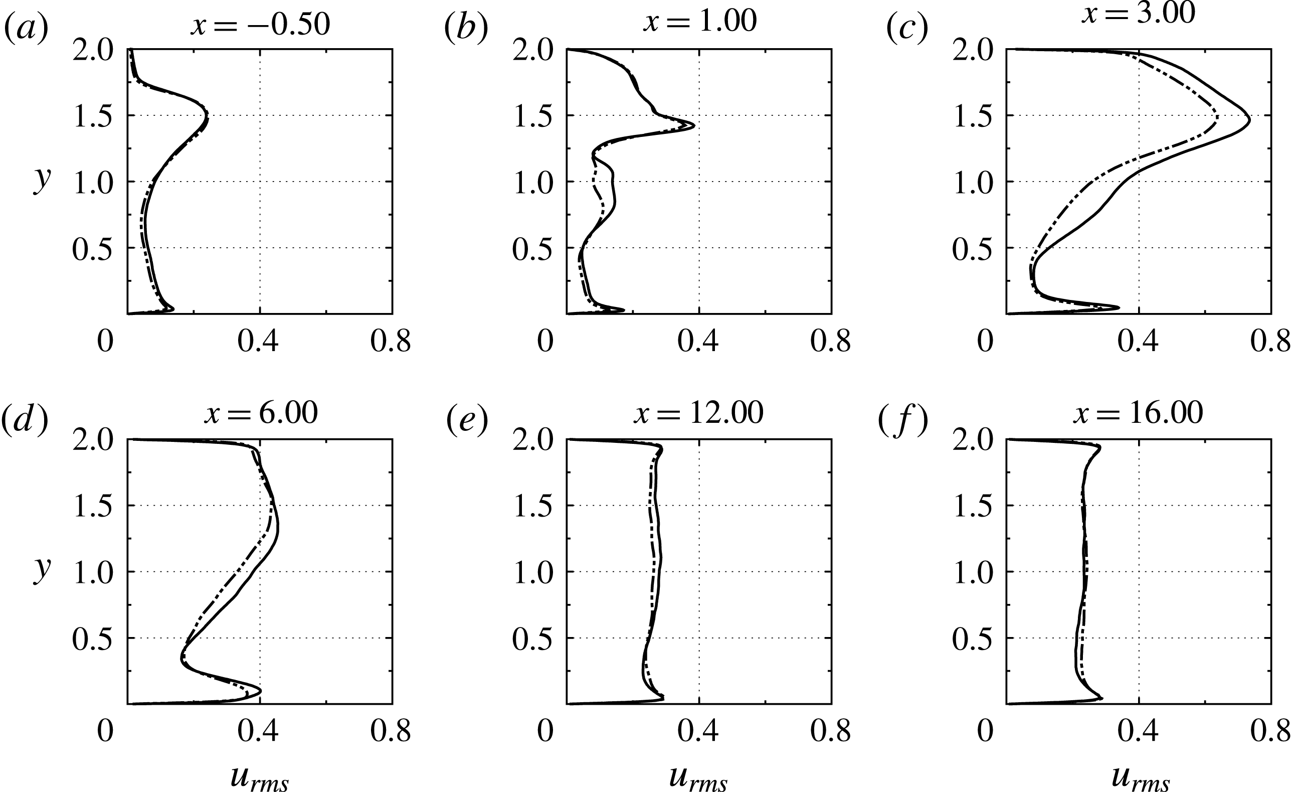
 $x=-0.50$
occurs at the core of the primary shear layer. At
 $x=1.0$
, due to the bending of the two streams, this shear layer is located lower down. The peak r.m.s. inside the shear layer occurs right below the mid-plane of the channel and its value is decreased due to the spreading of the layer. On the other hand, the strong peak at
 $y\approx 1.5$
corresponds to the secondary shear layer. We also observe that at
 $x=3.0$
the values of
 $u_{rms}$
have increased, which is attributed to turbulence generation inside the recirculation bubble and near the bottom wall due to the adverse pressure gradient. Further downstream,
 $u_{rms}$
becomes almost constant away from the walls and its profile starts to resemble the one in channel flows. By contrast, in the corresponding gas–gas flow, the wall-normal variations of
 $u_{rms}$
decay very slowly (Georgiou & Papalexandris Reference Georgiou and Papalexandris2017b
). This difference is due to the fact that the flow under study involves liquids and, therefore, buoyancy effects are less significant.
Profiles of the r.m.s. of the streamwise velocity
 $u_{rms}$
at different streamwise stations of the horizontal channel. ——, DNS; — ⋅ ⋅ —, LES.

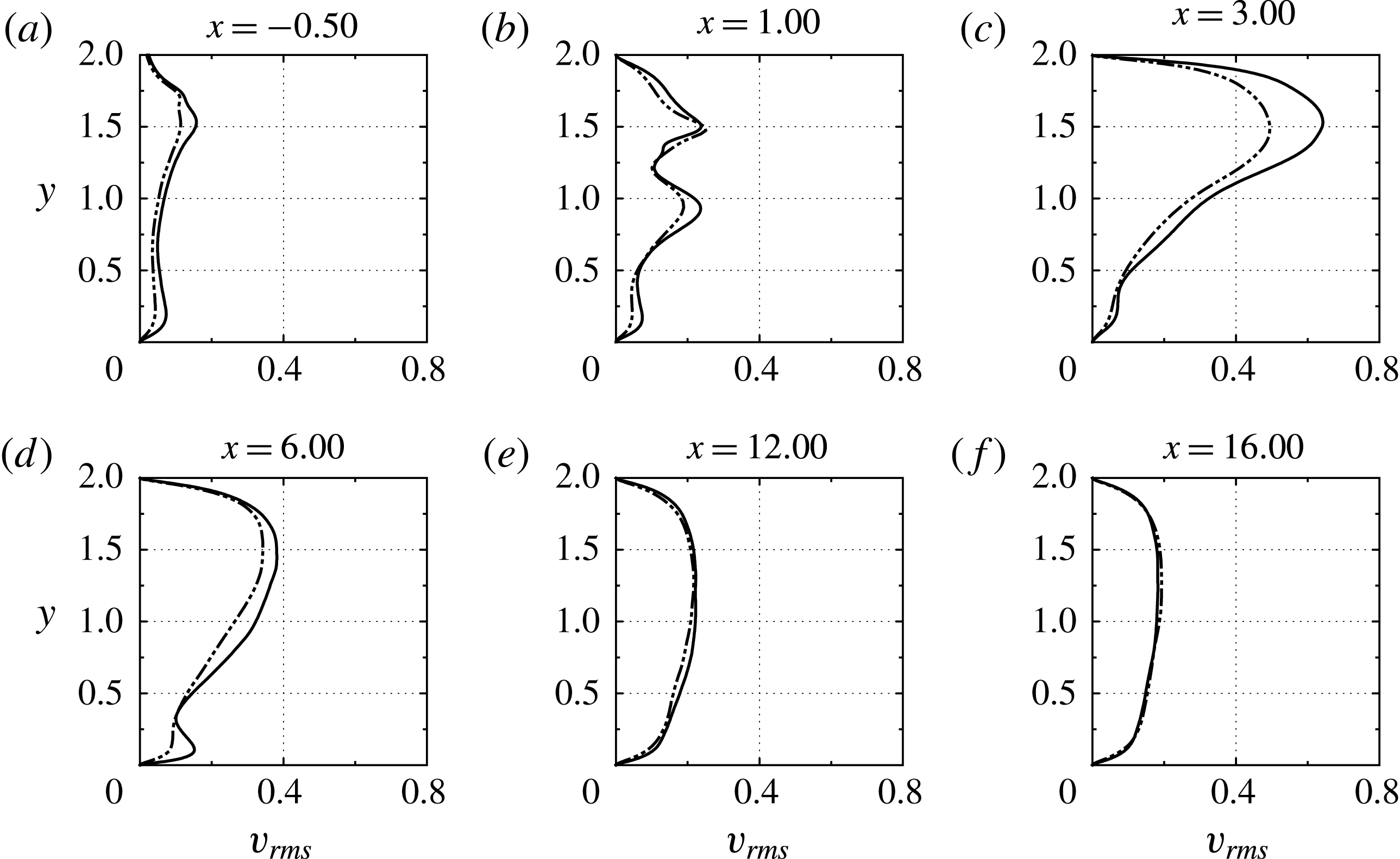
Profiles of the r.m.s. of the wall-normal velocity
 $v_{rms}$
at different streamwise stations of the horizontal channel. ——, DNS; — ⋅ ⋅ —, LES.

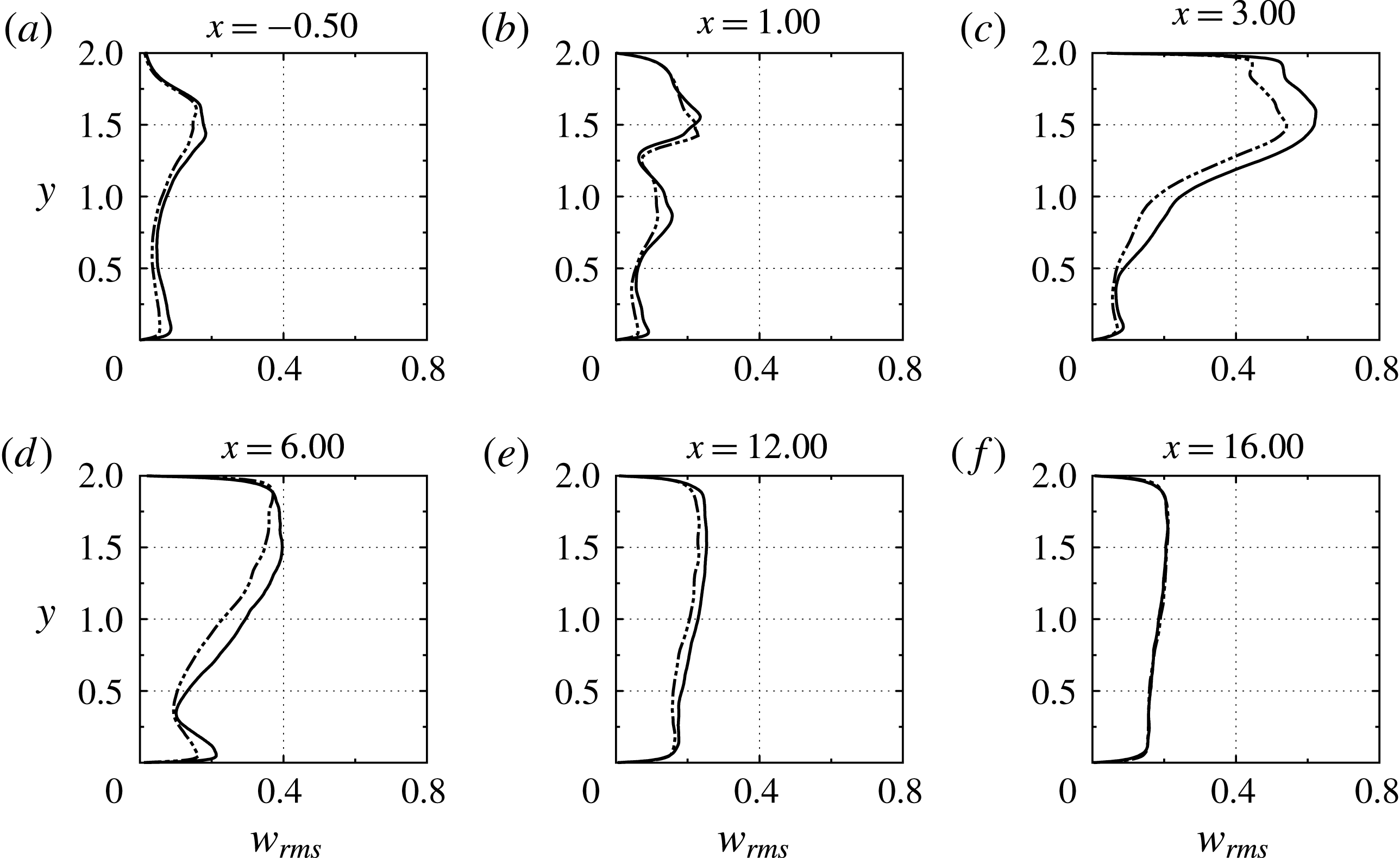
Profiles of the r.m.s. of the spanwise velocity
 $w_{rms}$
at different streamwise stations of the horizontal channel. ——, DNS; — ⋅ ⋅ —, LES.

The r.m.s. profiles of the wall-normal and spanwise velocities are shown in figures 17 and 18, respectively. At
 $x=-0.5$
, the peak of these profiles corresponds to the primary shear layer. Also, at the streamwise station
 $x=1.0$
, both
 $v_{rms}$
and
 $w_{rms}$
profiles exhibit a double-peak structure. The upper peak corresponds to the secondary and the lower peak to the primary shear layer. This structure was also observed in our simulations of gas–gas flow in T-junctions (Georgiou & Papalexandris Reference Georgiou and Papalexandris2017b
) but not in isothermal flows (Georgiou & Papalexandris Reference Georgiou and Papalexandris2017a
). We may therefore infer that this double peak is due to the role of the temperature as an active scalar. More specifically, the primary shear layer enhances significantly the mixing between the cross-flow and the incoming jet when these two streams are not at the same temperature. On the other hand, the large r.m.s. values inside the recirculation bubble, figures 17(c) and 18(c), are a common feature of both isothermal and variable-temperature flows in T-junctions. Further, from figures 16–18 we infer that the LES captures fairly well the r.m.s. profiles of all velocity components. Nonetheless, there are some discrepancies; most notably, it underpredicts the r.m.s. values inside the recirculation bubble by up to 25 %.
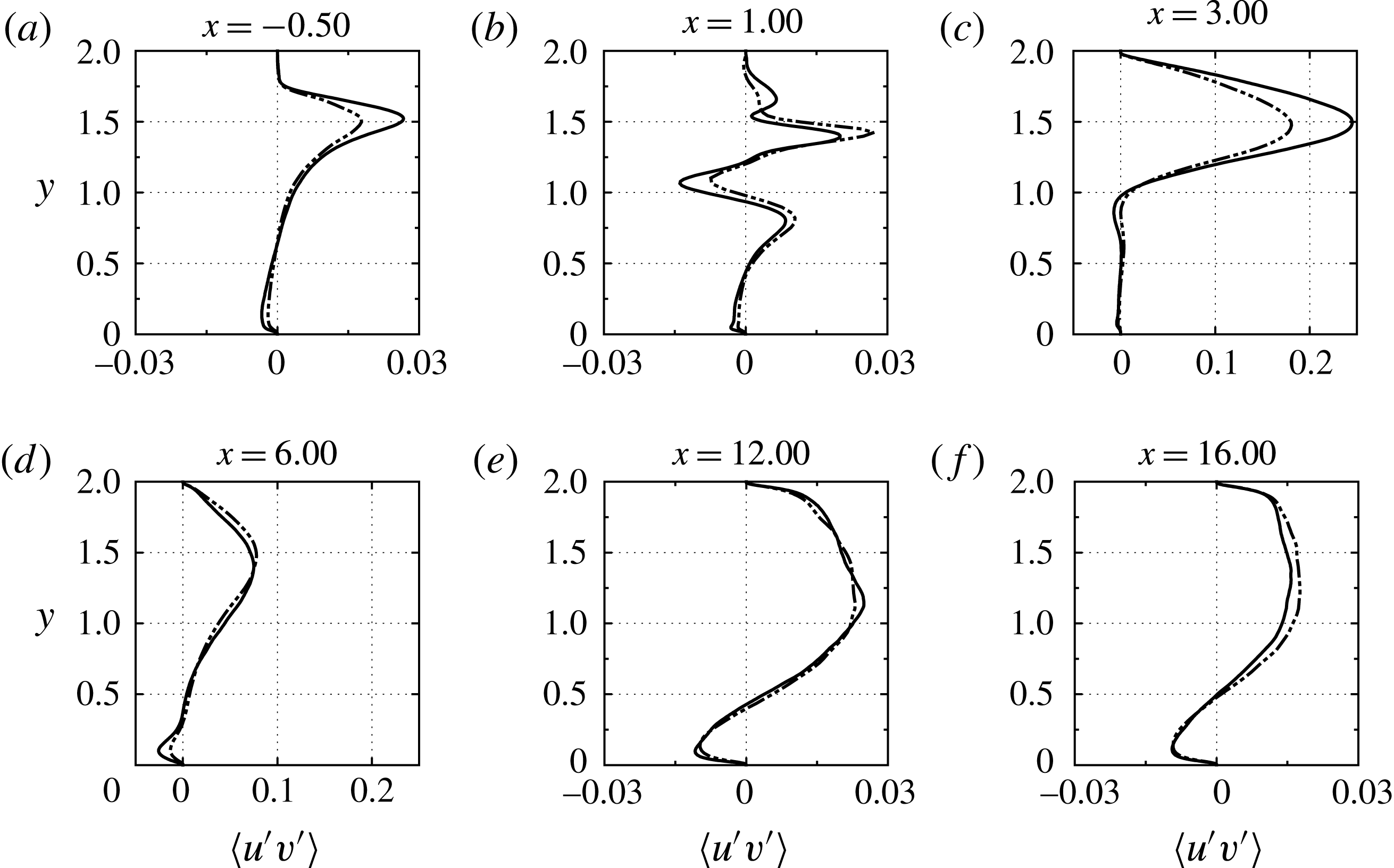
Next, in figure 19 we present results for the Reynolds shear stresses
 $\langle u^{\prime }v^{\prime }\rangle$
. At the streamwise station
 $x=1.0$
, they assume an S-shaped profile across the shear layers. Similar profiles have been predicted for shear layers at interfaces between pure fluids and porous media (Antoniadis & Papalexandris Reference Antoniadis and Papalexandris2015, Reference Antoniadis and Papalexandris2016). Herein, the large negative peak occurs at the core of the primary shear layer, whereas the large positive peak occurs at the core of the secondary layer. Further, the secondary peak at
 $x=1.0$
close to the top wall (
 $y\approx 1.75$
) is due to the secondary recirculation zone located next to the downstream corner of the entry of the jet, cf. figure 4.
Profiles of the Reynolds stress
 $\langle u^{\prime }v^{\prime }\rangle$
at different streamwise stations of the horizontal channel. ——, DNS; — ⋅ ⋅ —, LES. For purposes of clarity, the limits of the horizontal axis in (c) and (d) are different than in the other figures.

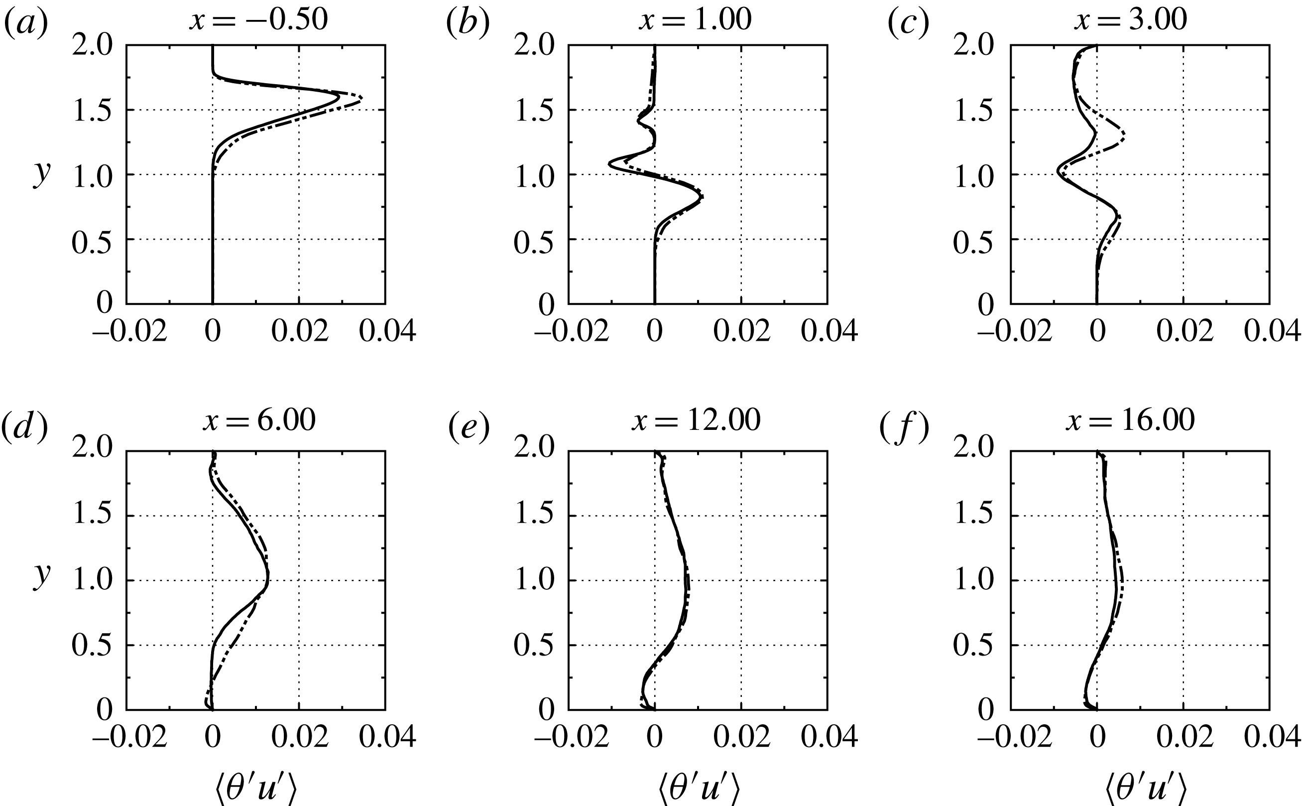
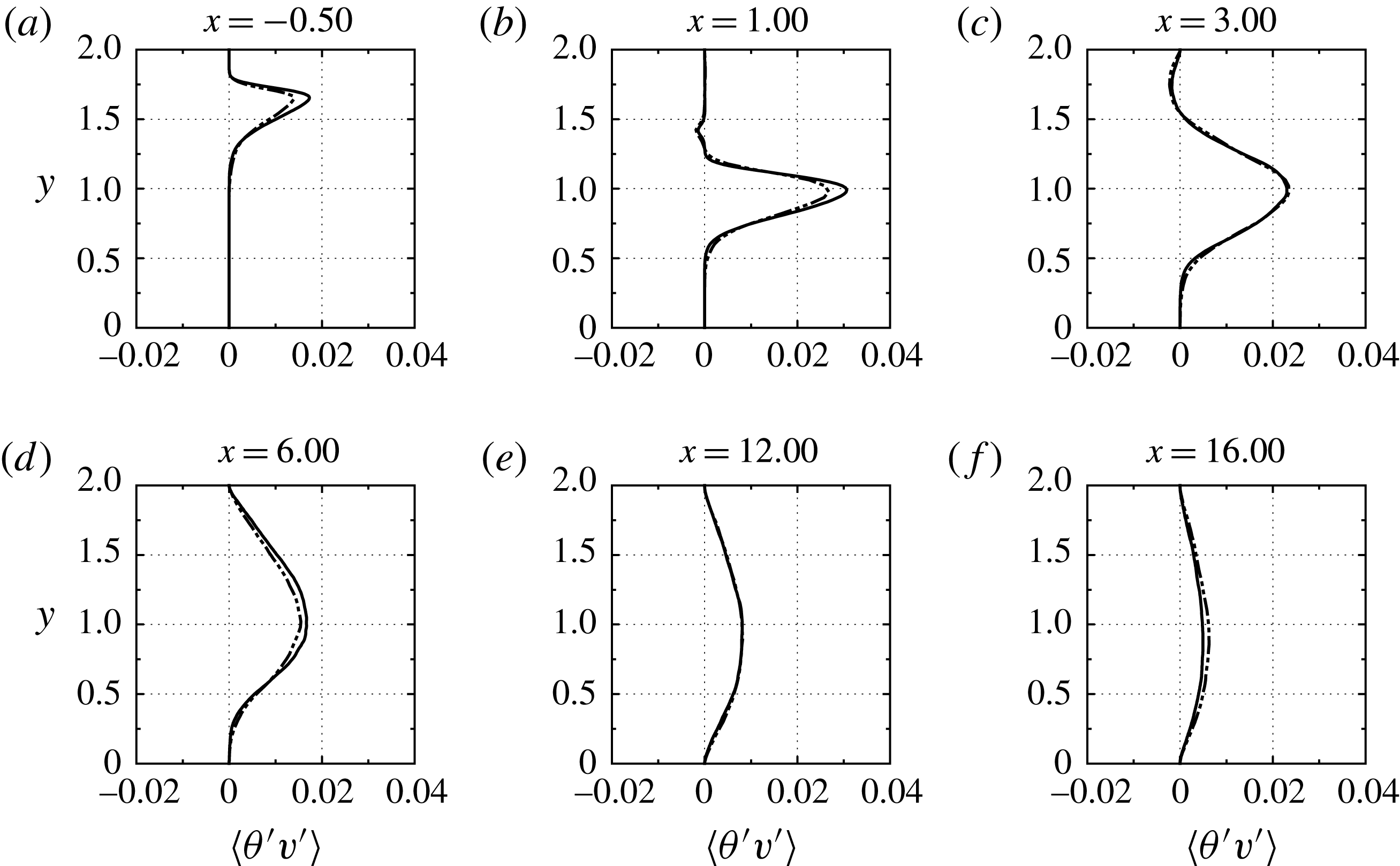
Our discussion of the flow statistics concludes with the results for the turbulent heat fluxes
 $\langle \unicode[STIX]{x1D703}^{\prime }u^{\prime }\rangle$
and
 $\langle \unicode[STIX]{x1D703}^{\prime }v^{\prime }\rangle$
. Their profiles at different streamwise stations are shown in figures 20 and 21, respectively. We observe that for
 $x<3$
, the peaks of these profiles occur at the core of the primary shear layer. In other words, the primary shear layer provides the main mechanism for thermal mixing. By comparison, the contribution of the secondary shear layer is very small. Further downstream, the amplitudes of both fluxes drop significantly as the merged shear layer spreads out. Another interesting point is that inside the recirculation bubble (
 $x=3.0$
), both turbulent fluxes are negative, i.e. they are directed upstream and downwards. This implies that, at this station, heat is transferred from the outer parts of the bubble toward its core. This is due to vortical structures emanating from the shear layers that get trapped inside the bubble.
Finally, we remark that the LES predictions agree fairly well with the DNS, especially as regards
 $\langle \unicode[STIX]{x1D703}^{\prime }v^{\prime }\rangle$
. The only noticeable disagreement is that the LES overpredicts the values of
 $\langle \unicode[STIX]{x1D703}^{\prime }u^{\prime }\rangle$
inside the recirculation bubble, and in the bottom half of the channel at
 $x=6.0$
. Based on the overall comparison of the first- and second-order statistics, we infer that the LES predictions for the flow under study are satisfactorily accurate, although there are some discrepancies in regions of intense turbulence production.
Profiles of the streamwise turbulent heat flux
 $\langle \unicode[STIX]{x1D703}^{\prime }u^{\prime }\rangle$
at different streamwise stations of the horizontal channel. ——, DNS; — ⋅ ⋅ —, LES.

Profiles of the wall-normal turbulent heat flux
 $\langle \unicode[STIX]{x1D703}^{\prime }v^{\prime }\rangle$
at different streamwise stations of the horizontal channel. ——, DNS; — ⋅ ⋅ —, LES.

3.3 Budget of the turbulent kinetic energy
In this subsection we analyse the budget of the turbulent kinetic energy (TKE) based on the DNS data. In order to fix ideas, let
 $K$
and
 $\bar{K}$
, denote the kinetic energy and the mean-flow kinetic energy, i.e.
 $K=(1/2)(\boldsymbol{u}\boldsymbol{\cdot }\boldsymbol{u})$
, and
 $\bar{K}=(1/2)(\langle \boldsymbol{u}\rangle \boldsymbol{\cdot }\langle \boldsymbol{u}\rangle )$
. The transport equation for TKE can be obtained by subtracting the equation for
 $\bar{K}$
from the one for
 $K$
(Chassaing et al.
Reference Chassaing, Antonia, Anselmet, Joly and Sarkar2002). However, when applied to variable-density flows, this procedure is quite cumbersome because it involves the density fluctuations. For this reason, it is customary to employ density-weighted averaging (Favre Reference Favre1983). For a generic quantity
 $\unicode[STIX]{x1D719}$
, the Favre average
 $\{\unicode[STIX]{x1D719}\}$
is defined as
 $$\begin{eqnarray}\displaystyle \{\unicode[STIX]{x1D719}\}=\frac{\langle \unicode[STIX]{x1D70C}\unicode[STIX]{x1D719}\rangle }{\langle \unicode[STIX]{x1D70C}\rangle }, & & \displaystyle\end{eqnarray}$$
and the Favre decomposition is then given by
 $$\begin{eqnarray}\displaystyle \unicode[STIX]{x1D719}=\{\unicode[STIX]{x1D719}\}+\unicode[STIX]{x1D719}^{\prime \prime }. & & \displaystyle\end{eqnarray}$$
An important feature of this decomposition is that the fluctuating component
 $\unicode[STIX]{x1D719}^{\prime \prime }$
is not centred, i.e.
 $\langle \unicode[STIX]{x1D719}^{\prime \prime }\rangle \neq 0$
. Relationships between the standard and Favre averaging operations can be found in Huang, Coleman & Bradshaw (Reference Huang, Coleman and Bradshaw1995) and Chassaing et al. (Reference Chassaing, Antonia, Anselmet, Joly and Sarkar2002). Let
 $k$
denote the turbulence kinetic energy of the density-weighted velocity fluctuations,
 $$\begin{eqnarray}\displaystyle k={\textstyle \frac{1}{2}}(\boldsymbol{u}^{\prime \prime }\boldsymbol{\cdot }\boldsymbol{u}^{\prime \prime }). & & \displaystyle\end{eqnarray}$$
Then the Favre-averaged turbulent kinetic energy,
 $\{k\}=(1/2)\{\boldsymbol{u}^{\prime \prime }\boldsymbol{\cdot }\boldsymbol{u}^{\prime \prime }\}$
, satisfies the following transport equation (Chassaing et al.
Reference Chassaing, Antonia, Anselmet, Joly and Sarkar2002),
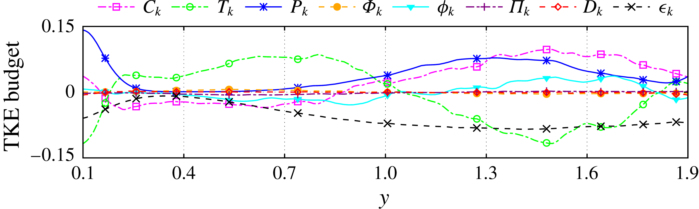
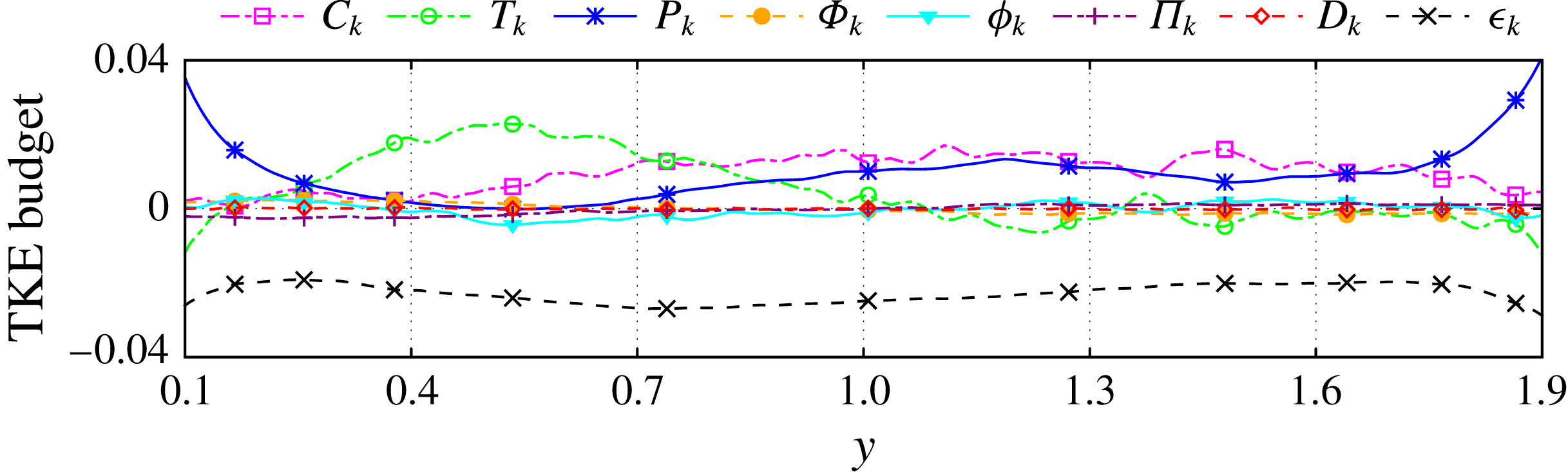
 $$\begin{eqnarray}\displaystyle \frac{\unicode[STIX]{x2202}\langle \unicode[STIX]{x1D70C}\rangle \{k\}}{\unicode[STIX]{x2202}t} & = & \displaystyle -\underbrace{\unicode[STIX]{x1D735}\boldsymbol{\cdot }(\langle \unicode[STIX]{x1D70C}\rangle \{k\}\{\boldsymbol{u}\})}_{C_{k}}-\underbrace{\langle \unicode[STIX]{x1D70C}\rangle \{\boldsymbol{u}^{\prime \prime }\boldsymbol{u}^{\prime \prime }\}\boldsymbol{ : }\unicode[STIX]{x1D735}\{\boldsymbol{u}\}}_{P_{k}}\nonumber\\ \displaystyle & & \displaystyle -\,\underbrace{\unicode[STIX]{x1D735}\boldsymbol{\cdot }(\langle \unicode[STIX]{x1D70C}\rangle \{k\,\boldsymbol{u}^{\prime \prime }\})}_{T_{k}}-\underbrace{\unicode[STIX]{x1D735}\boldsymbol{\cdot }(\langle p\rangle \langle \boldsymbol{u}^{\prime \prime }\rangle )}_{\unicode[STIX]{x1D6F7}_{k}}-\underbrace{\unicode[STIX]{x1D735}\boldsymbol{\cdot }\langle p^{\prime }\boldsymbol{u}^{\prime \prime }\rangle }_{\unicode[STIX]{x1D719}_{k}}\nonumber\\ \displaystyle & & \displaystyle +\,\underbrace{\langle p\,\unicode[STIX]{x1D735}\boldsymbol{\cdot }\langle \boldsymbol{u}^{\prime \prime }\rangle \rangle }_{\unicode[STIX]{x1D6F1}_{k}}+\underbrace{\frac{1}{Re}\unicode[STIX]{x1D735}\boldsymbol{\cdot }\langle \unicode[STIX]{x1D749}\boldsymbol{\cdot }\boldsymbol{u}^{\prime \prime }\rangle }_{D_{k}}-\underbrace{\frac{1}{Re}\langle \unicode[STIX]{x1D749}\boldsymbol{ : }\unicode[STIX]{x1D735}\boldsymbol{u}^{\prime \prime }\rangle }_{\unicode[STIX]{x1D716}_{k}}.\end{eqnarray}$$
In the above equation,
 $C_{k}$
describes convection of TKE, while
 $P_{k}$
and
 $T_{k}$
describe production and transport of TKE, respectively. The terms
 $\unicode[STIX]{x1D6F7}_{k}$
and
 $\unicode[STIX]{x1D719}_{k}$
describe the work of the mean and fluctuating pressures through fluctuating motions, respectively. Also,
 $\unicode[STIX]{x1D6F1}_{k}$
represents the pressure correlation with the dilatation fluctuation. Finally,
 $D_{k}$
describes the viscous diffusion, which is the work of viscous stresses through fluctuating motions, whereas
 $\unicode[STIX]{x1D716}_{k}$
describes viscous dissipation. It should be mentioned that the work of the gravitational force does not enter the above equation.
It is also worth noting that since the fluid viscosity is temperature dependent, one could insert the expression (2.4) for
 $\unicode[STIX]{x1D749}$
in the last two terms of equation (3.6) and further expand these terms. This expansion results in terms involving triple moments and, as shown by Huang et al. (Reference Huang, Coleman and Bradshaw1995), allows for a more detailed description of the TKE budget. In particular, it provides the specific contribution of the fluctuating component of
 $\unicode[STIX]{x1D749}$
. Other authors such as Lessani & Zainali (Reference Lessani and Zainali2009) opted not to expand the last two terms of (3.6). In the present study we follow the approach of Lessani & Zainali (Reference Lessani and Zainali2009) for purposes of simplicity of the analysis. Conversely, Zonta et al. (Reference Zonta, Marchioli and Soldati2012) followed yet another approach and excluded altogether the contribution of viscosity fluctuations in the TKE budget.
In statistically stationary flows, the sum of all the terms at the right-hand side of equation (3.6) is zero. Indeed, the computed value of this sum from the DNS data is always very small and below 5 % of the amplitude of the largest term of (3.6), which is as an indication of the accuracy of our DNS. Further, since this computed sum is negligible, we have not included it in the figures for purposes of clarity of the plots.
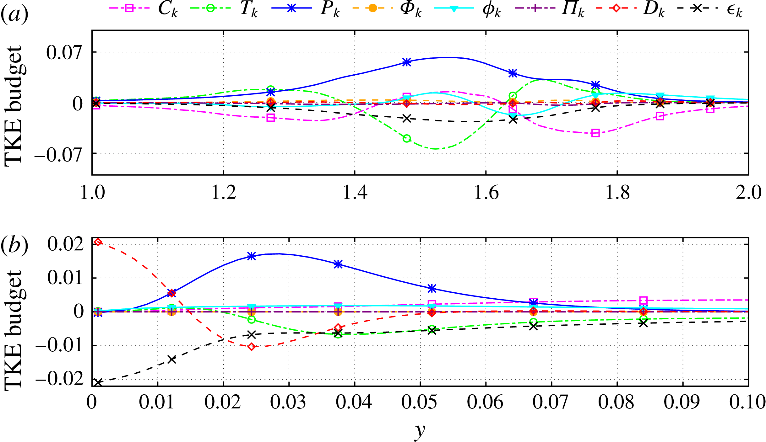
In figure 22 we present the TKE budget across the channel at
 $x=-0.5$
. At this station, the main source of turbulence production is the primary shear layer, which can be confirmed by the high values of
 $P_{k}$
therein. Also,
 $T_{k}$
takes negative values inside this shear layer, which implies transport of turbulent kinetic energy from the core of the layer toward its edges. On the other hand, the turbulent convection term
 $C_{k}$
follows the opposite trend since it is positive at the core and negative at the edges of the primary shear layer. As concerns the turbulent dissipation
 $\unicode[STIX]{x1D716}_{k}$
, it is approximately 3 times smaller than
 $P_{k}$
. The high ratio between the production and dissipation terms,
 $P_{k}/\unicode[STIX]{x1D716}_{k}\approx 3$
, corroborates the fact that, with respect to turbulent kinetic energy, the flow at this region is far from equilibrium.
Budget of the turbulent kinetic energy at the streamwise station
 $x=-0.5$
. (a) Bulk of the channel, (b) close up look at the bottom wall.

The TKE budget at
 $x=-0.5$
and close to the bottom wall is shown in figure 22(b). Therein, the boundary layer is subject to a favourable pressure gradient due to the aforementioned Venturi effect. The peak of the production term
 $P_{k}$
occurs at
 $y^{+}\approx 10$
; this is somewhat lower than the location
 $y^{+}\approx 12$
of the corresponding peak in zero-pressure-gradient boundary layers (Kim, Moin & Moser Reference Kim, Moin and Moser1987; Spalart Reference Spalart1988). Further, the production term is mostly balanced by the work of the fluctuating viscous forces
 $D_{k}$
. Finally, as expected, closer to the wall all terms vanish except for
 $D_{k}$
which is balanced by the viscous dissipation.
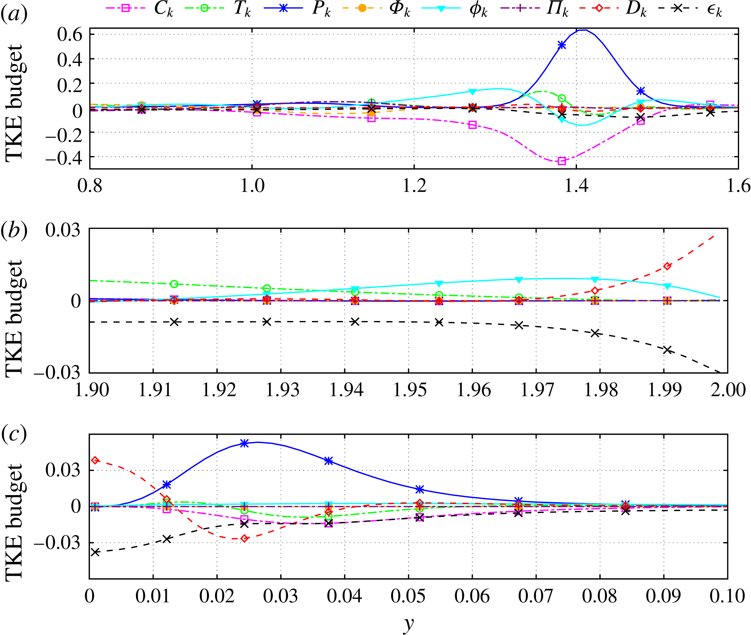
The profiles of the TKE budget at
 $x=1.0$
are plotted in figure 23. The main features of the budget are the high amplitudes of the production and convection terms in the zone occupied by the secondary shear layer. In fact, the peak of the production term is an order of magnitude higher than the one at
 $x=-0.5$
, which confirms that the interaction of the incoming jet with the recirculation bubble is a major source of turbulence generation. Also, the negative values of the convection term
 $C_{k}$
imply that TKE is convected from the core of secondary shear layer toward its edges and the core of the bubble. At the bottom wall, the pressure gradient is still favourable. Therefore, the profiles of the terms of the TKE budget are similar to those at
 $x=-0.5$
.
Budget of the turbulent kinetic energy at the streamwise station
 $x=1.0$
. (a) Bulk of the channel, (b) close up look at the top wall, (c) close up look at the bottom wall.

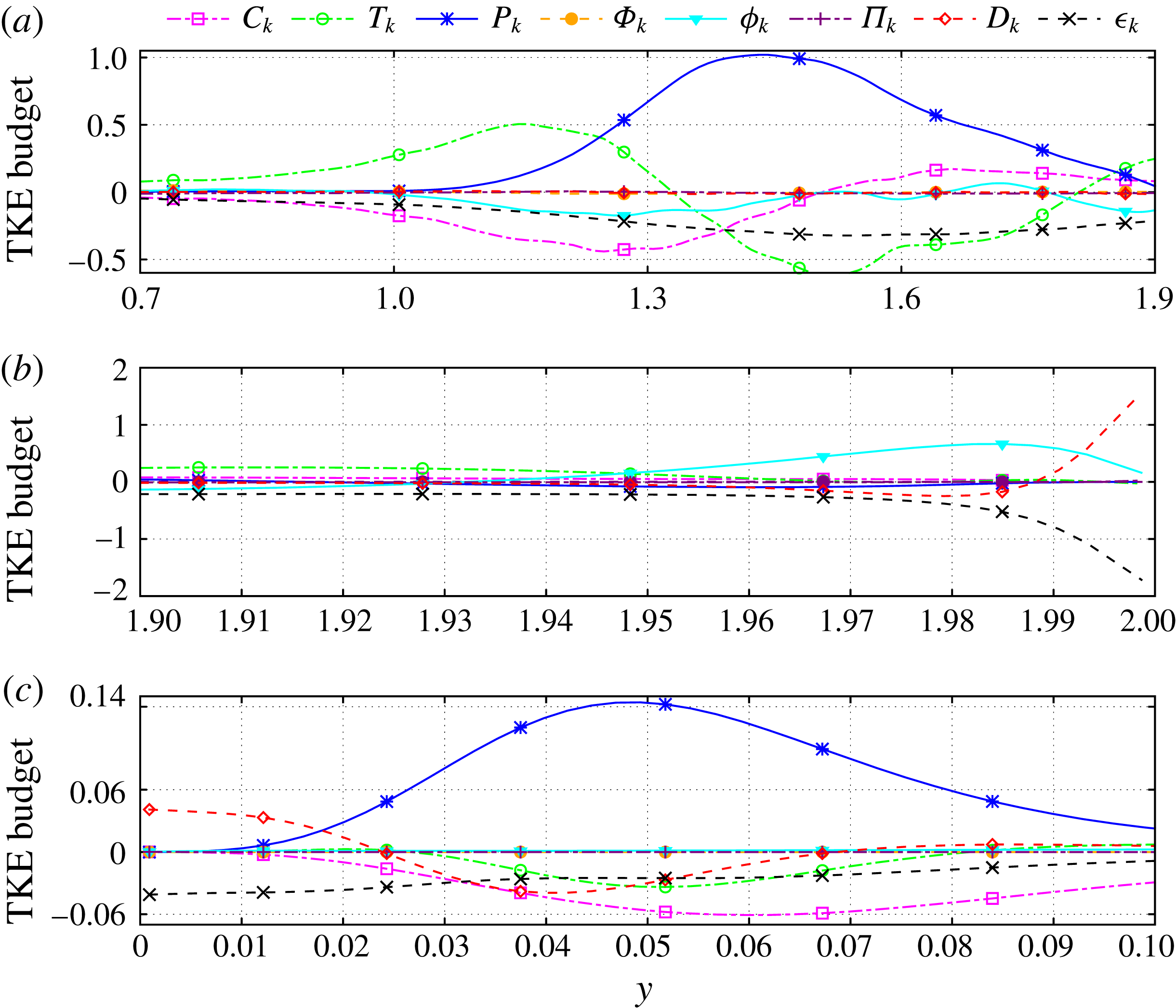
The TKE budget at
 $x=3.0$
is presented in figure 24. The spreading of the shear layers and their merging lead to even higher values of turbulence production above the mid-plane. Also, the peak value of
 $P_{k}$
is considerably higher; this is in accordance with the high r.m.s. velocities at this station that are plotted in figures 16–19. The production term is balanced by turbulence transport, convection and dissipation. Interestingly, the convection term
 $C_{k}$
takes negative values close to the mid-plane. However, inside the recirculation bubble it changes sign and becomes positive, which implies convective transport of turbulent kinetic energy from the reattachment region toward the centre of the bubble. This has also been observed in the simulations of flow in channel with constrictions by Fröhlich et al. (Reference Fröhlich, Mellen, Rodi, Temmerman and Leschziner2005). Also, near the bottom wall, the cross-flow is subject to the adverse pressure gradient which results to large turbulence generation; see figure 24(c). In fact, the near-wall peak of
 $P_{k}$
, located at
 $y^{+}\approx 12$
, is 3 times higher than the corresponding peak at the upstream station
 $x=1.0$
. Moreover, according to figure 24(c), the near-wall turbulence production is mostly balanced by
 $C_{k}$
,
 $D_{k}$
and
 $\unicode[STIX]{x1D716}_{k}$
.
Budget of the turbulent kinetic energy at the streamwise station
 $x=3.0$
. (a) Bulk of the channel, (b) close up look at the top wall, (c) close up look at the bottom wall.

Budget of the turbulent kinetic energy at the streamwise station
 $x=6.0$
.

Downstream of the reattachment point of the flow, the amplitudes of all the terms in the TKE equation (3.6) decrease with
 $x$
. In figure 25 we have plotted the TKE budget at
 $x=6.0$
. We observe that
 $T_{k}$
is positive above and negative below the mid-plane, which implies transport of turbulent kinetic energy away from the walls and toward the bulk of the channel. Additionally, the ratio
 $P_{k}/\unicode[STIX]{x1D716}_{k}$
is close but not equal to unity. At the same time, due to the spreading of the merged shear layer downstream of the recirculation bubble, the convective and transport terms are also significant and of the same order of magnitude as
 $P_{k}$
and
 $\unicode[STIX]{x1D716}_{k}$
. Moreover, nowhere in the flow field is
 $P_{k}$
counter-balanced by
 $\unicode[STIX]{x1D716}_{k}$
alone. This implies that, even when the ratio
 $P_{k}/\unicode[STIX]{x1D716}_{k}$
gets close to unity, the flow turbulence is not at equilibrium.
Finally, in figure 26 we provide the TKE budget far downstream, at the station
 $x=12.0$
. We can readily observe that as the flow evolves, the amplitudes of the various terms in the TKE budget decrease even further. Moreover, the profiles at the near-wall regions, which are not shown herein for purposes of economy of space, start to resemble those of zero-pressure-gradient boundary layers; see, for example, Kim et al. (Reference Kim, Moin and Moser1987) and Spalart (Reference Spalart1988).
Budget of the turbulent kinetic energy at the streamwise station
 $x=12.0$
.

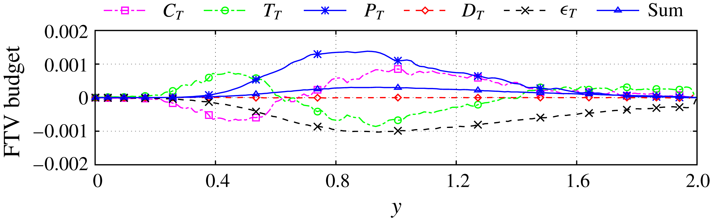
Budget of the fluctuating temperature variance (FTV) at the streamwise station
 $x=-0.5$
.

3.4 Budget of the fluctuating temperature variance
In this subsection we analyse the budget of the fluctuating temperature variance (FTV) at different streamwise locations based on the DNS data. The transport equation for FTV,
 $(T^{\prime \prime }T^{\prime \prime })/2$
, can be derived by first multiplying every term of (2.3) with
 $T$
so as to obtain an equation for
 $T^{2}$
, then by Favre averaging the result in order to derive an equation for
 $\{T^{2}\}$
and, finally, by subtracting the equations for
 $T^{2}$
and
 $\{T^{2}\}$
. The resulting transport equation reads
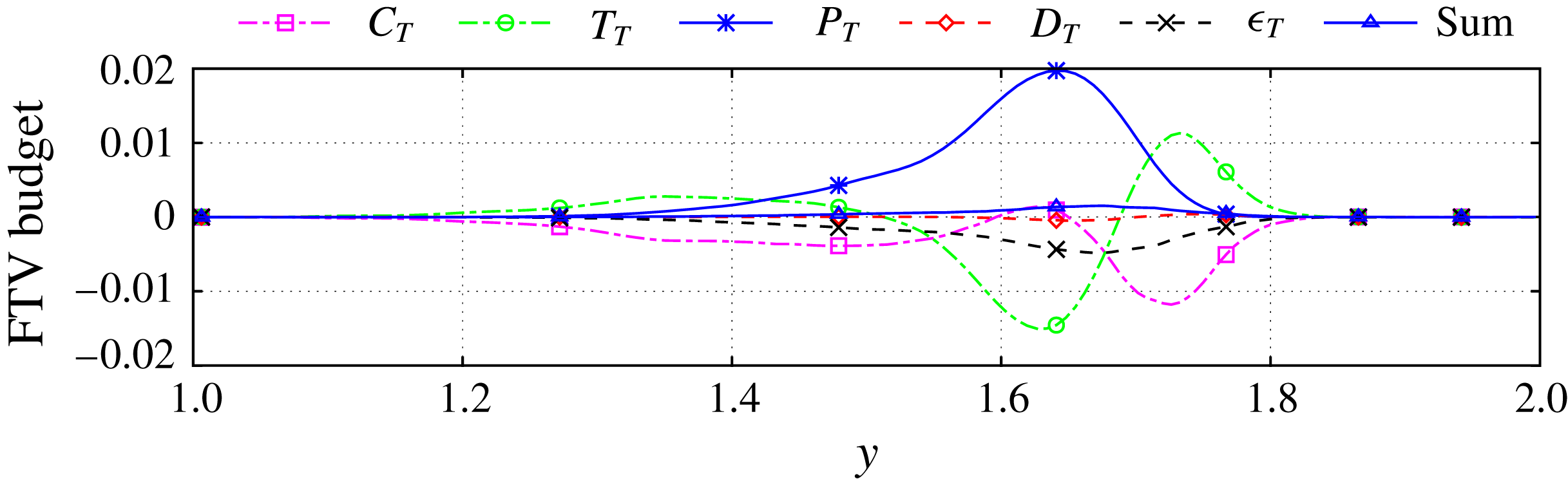
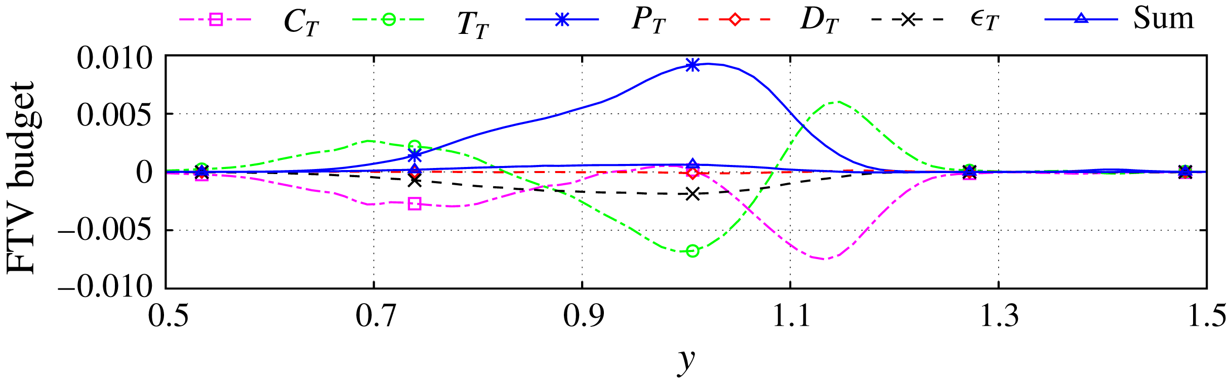
 $$\begin{eqnarray}\displaystyle & & \displaystyle \frac{1}{2}\frac{\unicode[STIX]{x2202}(\langle \unicode[STIX]{x1D70C}\rangle \{T^{\prime \prime }T^{\prime \prime }\})}{\unicode[STIX]{x2202}t}=-\frac{1}{2}\underbrace{\unicode[STIX]{x1D735}\boldsymbol{\cdot }(\langle \unicode[STIX]{x1D70C}\rangle \{T^{\prime \prime }T^{\prime \prime }\}\{\boldsymbol{u}\})}_{C_{T}}-\underbrace{\langle \unicode[STIX]{x1D70C}\rangle \{T^{\prime \prime }\boldsymbol{u}^{\prime \prime }\}\boldsymbol{\cdot }\unicode[STIX]{x1D735}\{T\}}_{P_{T}}\nonumber\\ \displaystyle & & \displaystyle \qquad -\,\frac{1}{2}\underbrace{\unicode[STIX]{x1D735}\boldsymbol{\cdot }(\langle \unicode[STIX]{x1D70C}\rangle \{T^{\prime \prime }T^{\prime \prime }\,\boldsymbol{u}^{\prime \prime }\})}_{T_{T}}+\underbrace{\frac{1}{Re\,Pr}\unicode[STIX]{x1D735}\boldsymbol{\cdot }\langle T^{\prime \prime }\unicode[STIX]{x1D705}\unicode[STIX]{x1D735}T\rangle }_{D_{T}}-\underbrace{\frac{1}{Re\,Pr}\langle \unicode[STIX]{x1D705}\unicode[STIX]{x1D735}T\boldsymbol{\cdot }\unicode[STIX]{x1D735}T^{\prime \prime }\rangle }_{\unicode[STIX]{x1D716}_{T}}.\end{eqnarray}$$
In the above equation, the terms
 $C_{T}$
,
 $P_{T}$
and
 $T_{T}$
describe convection, production and transport of fluctuating temperature variance, respectively. Further,
 $D_{T}$
describes viscous transport, whereas
 $\unicode[STIX]{x1D716}_{T}$
describes viscous dissipation of FTV. Similarly to the TKE equation (3.6) one could expand the last two terms in the above equation even further so as to obtain terms that involve the fluctuating component of the heat flux vector
 $\unicode[STIX]{x1D705}\unicode[STIX]{x1D735}T$
. As in the case of the TKE equation, we opt not to follow this approach for purposes of simplicity of the analysis; in any case, in the flow under study the ratio between the conductivities of the two streams is small (approximately equal to 1.15).
Once the flow becomes statistically stationary, the sum of all the terms at the right-hand side of the above equation is zero. Indeed, the computed value of this sum based on the DNS data is small and below 20 % of the amplitude of the largest term.
In figure 27 we show plots of the terms at the right-hand side of (3.7) at the streamwise station
 $x=-0.5$
. We see that the various terms of the budget become significant only across the primary shear layer, which provides the main mechanism for thermal mixing. The peak of the production term occurs at the core of this shear layer and is counter-balanced by the transport term and, to a lesser extent, by the dissipation term. We also observe that near the edges of this shear layer, the convection and transport terms are of opposite sign and they essentially cancel each other out. At the same time, the values of the viscous transport term
 $D_{T}$
are very small compared to those of the other terms.
The same observations hold for the budget of the FTV at
 $x=1.0$
, which is shown in figure 28. Moreover, at this streamwise location the profiles of the various terms have ‘spread out’ and their values have decreased due to the spreading of the primary shear layer. In figure 29 we have plotted the FTV budget further downstream, at
 $x=6.0$
. We readily infer that the amplitudes of all terms, have decreased even further. On the other hand, the relative strength of the dissipation term
 $\unicode[STIX]{x1D716}_{T}$
has increased so that it almost counter-balances the production term
 $P_{T}$
. At the same time, the convective and transport terms have opposite signs and almost equal amplitudes so that they essentially cancel each other out. Finally, according to our simulation, as the thermal mixing evolves, all the terms in the FTV budget decrease substantially further downstream.
Budget of the fluctuating temperature variance (FTV) at the streamwise station
 $x=1.0$
.

Budget of the fluctuating temperature variance (FTV) at the streamwise station
 $x=6.0$
.

3.5 Spectral analysis of the velocity and temperature signals
We proceed with the spectral analysis of the velocity and temperature signals at two locations of interest. The first one is at
 $(x,y)=(-0.5,\,1.6)$
, i.e. beneath the entry of the jet and at the interface of the two streams. The second location is
 $(x,y)=(12.0,\,1.0)$
, i.e. far downstream of the recirculation bubble and at the mid-plane. Our procedure is the following. Once the flow has become statistically stationary, we record the time signals of the spanwise-averaged velocity components
 $\overline{u}$
and
 $\overline{v}$
and temperature
 $\overline{T}$
at the above locations for 40 non-dimensional time units. Then, we compute the power spectral densities,
 $S_{uu}(f)$
,
 $S_{vv}(f)$
and
 $S_{TT}(f)$
, of these signals so as to estimate the characteristic frequencies
 $f$
with which they oscillate. The frequency is then normalised with respect to the half-width of the horizontal channel and the bulk velocity of the cross-flow, which provides the corresponding Strouhal number
 $St=f\unicode[STIX]{x1D6FF}/U_{c}$
.
Power spectral density of the spanwise-averaged signals
 $\overline{u}$
,
 $\overline{v}$
and
 $\overline{T}$
, at two locations in the horizontal channel. Each profile has been normalised with respect to its maximum value. (a)
 $(x,\,y)=(-0.5,\,1.6)$
, (b)
 $(x,\,y)=(12.0,\,1.0)$
.

Figure 30 shows the power spectral densities at these two locations. At the first one,
 $(x,y)=(-0.5,\,1.6)$
, they all exhibit three low-
 $St$
peaks, at
 $St=0.035,\,0.09$
and 0.15. Further, the peaks of
 $S_{uu}$
and
 $S_{vv}$
occur at the same frequencies. These peaks are thus attributed to the oscillatory motion of the primary shear layer and to its shedding of vortices. Also, the three low-
 $St$
peaks of
 $S_{TT}$
occur at slightly different Strouhal numbers than those of
 $S_{uu}$
and
 $S_{vv}$
; this is due to the fact that thermal mixing at this location is still at an early stage and, therefore, the fluctuations of the temperature are not yet synchronised with those of the velocity. We further observe that the profile of
 $S_{TT}$
has a strong peak at a higher Strouhal number,
 $S_{t}\approx 0.5$
, in contrast to the profiles of
 $S_{uu}$
and
 $S_{vv}$
. Based on the video animations of the DNS (see the supplementary movies), we may attribute this peak to the wrapping of fluid of different temperature by the mushroom-like structures at the interface of the two streams such as the ones depicted in figure 10(a).
On the other hand, at the second location
 $(x,y)=(12.0,\,1.0)$
, the peaks of the power spectral densities occur at the same frequencies. In other words, the dominant frequencies of the oscillatory motion of
 $u$
,
 $v$
and
 $T$
coincide. The synchronisation of the power spectral densities is due to the extent of thermal mixing that has taken place. It also implies that once the two streams have been aligned sufficiently downstream of the recirculation bubble, the convective motions of spanwise vortices provide the main mechanism for thermal mixing.
4 Conclusions
In this article we presented an analysis of turbulent heat transfer in liquid–liquid flows in a T-junction under non-Boussinesq conditions. Our study was based on DNS of the interaction and thermal mixing between a hot incoming cross-flow and a cold vertical jet coming from above, supplemented with wall-resolved LES of the same flow. According to our simulations, both thermal mixing and turbulence production are driven by the two shear layers that originate from the corners of the entry of the jet, i.e. the primary shear layer that is formed by the two streams and the secondary shear layer that is formed by the incoming jet and the large recirculation bubble. These two layers roll up rapidly, thereby shedding numerous spanwise and streamwise vortical structures. Most of them break up in small vortices that are convected downstream in a highly turbulent environment, whereas others are trapped in the recirculation bubble. As the two shear layers spread, they start to interact and eventually merge, which further enhances mixing and heat diffusion. Our analysis of the turbulent-kinetic-energy budget further corroborates the dominant role of these shear layers in turbulence production and transport. Most of the turbulent kinetic energy is dissipated at the walls of the horizontal channel with particularly high values recorded close to the reattachment point of the flow. Further downstream, the ratio between the production and dissipation of turbulent kinetic energy become close to unity. At the same time, however, the convection and transport terms are of the same order as the production and dissipation terms, which implies that the turbulence does not reach equilibrium.
Another important feature of the flow is that the recirculation bubble leads to a Venturi effect that produces a favourable pressure gradient and accelerates both cross-flow and incoming jet. Subsequently though, as the flow expands, an adverse pressure gradient is formed which contributes considerably to turbulence generation, especially in the bottom half of the horizontal channel. Our simulations further reveal that the flow at the vertical branch detaches before it enters the horizontal channel, which leads to the formation a secondary recirculation zone inside the vertical channel. Also, due to its high momentum flux, part of the incoming jet bends upstream upon entry in the horizontal channel, which produces a thin and elongated separation zone close to the top wall.
The comparisons of our simulations revealed that the wall-resolved LES provides satisfactory predictions the first- and second-order statistics of the flow quantities. The most noticeable discrepancy is that the LES produced mildly diffused profiles for the second-order statistics in the regions of intense turbulence production, such as the large recirculation bubble. Even so, these discrepancies are not deemed detrimental, given the significant computational savings that LES offers.
Acknowledgements
The authors gratefully acknowledge the financial support of Bel V, a subsidiary of the Belgian Federal Agency of Nuclear Control. Further, they thank Professor B. Lessani for many fruitful discussions.
Supplementary movies
Supplementary movies are available at https://doi.org/10.1017/jfm.2018.256.