



1 Introduction and main result
1.1 Model and synopsis of related studies
This article focuses on the following compressible magnetohydrodynamic (MHD) system without shear viscosity, given by

where
 $\mathbb T^2$
denotes the two-dimensional periodic torus. Here,
 $\rho =\rho (t,x)$
,
 $ \mathbf {u} = \mathbf {u} (t,x),$
and
 $\mathbf {B}= \mathbf {B} (t,x)$
represent the fluid density, velocity field, and the magnetic field, respectively. The pressure
 $P=P(\rho )$
is a function of the density, which is assumed to be smooth and strictly increasing. The constant
 $\nu>0$
is the bulk viscosity coefficient, and
 $\sigma>0$
is the electrical conductivity of the field.
The MHD system (1.1) possesses a special equilibrium state characterized by a constant density, a zero velocity field, and a background magnetic field. This article aims to conduct a perturbation analysis around this state, investigating fundamental questions, such as global existence, stability, and large-time asymptotic behavior. Our study is motivated by two primary factors. First, we seek to provide a rigorous mathematical explanation for the experimentally observed stabilizing effect of a background magnetic field (see, e.g., [Reference Alexakis1–Reference Bardos, Sulem and Sulem3, Reference Chen, Zhang and Zhou5, Reference Gallet, Berhanu and Mordant14, Reference Gallet and Doering15, Reference Zhai44]). Second, we address the inherent mathematical challenges caused by the absence of shear viscosity in the system. The lack of uniform ellipticity, when only bulk viscosity is present, significantly complicates the control of nonlinear terms and demands novel analytical approaches.
We outline some physical background for the system (1.1). The dynamics of electrically conducting fluids interacting with magnetic fields are governed by the MHD equations. Compressible MHD models serve as the fundamental framework for theoretically describing turbulence in the solar wind [Reference Tandberg-Hanssen and Emslie35]. Since observed fluctuations often involve density variations, plasma compressibility effects must be considered in the theory. In standard MHD theory, the momentum equation includes both shear viscosity and volume viscosity, namely,
 $$ \begin{align} \left\{\begin{aligned} &\partial_t \rho + {\mathrm{div}} (\rho \mathbf{u}) =0, \\ &\rho\partial_t \mathbf{u}+ \rho\mathbf{u}\cdot\nabla \mathbf{u}-\mu\Delta \mathbf{u} - \nu \nabla {\mathrm{div}} \mathbf{u}+\nabla P=(\nabla\times\mathbf{B})\times\mathbf{B},\\ &\partial_t \mathbf{B}-\sigma\Delta \mathbf{B}+\mathbf{u}\cdot\nabla\mathbf{B}-\mathbf{B}\cdot\nabla\mathbf{u}+\mathbf{B} \text{ div}\, \mathbf{u}=0,\\ &{\mathrm{div}} \mathbf{B} =0,\\ &(\rho, \mathbf{u} ,\mathbf{B})|_{t=0}=(\rho_0, \mathbf{u} _0,\mathbf{B}_0), \end{aligned}\right. \end{align} $$
where
 $\mu \ge 0$
is the shear viscosity coefficient. In general, shear viscosity coefficient
 $\mu $
in the system (1.2) plays a central role in the study of fluid dynamics. Ultimately, it is the source of all forms of loss and drag and gives rise to the instabilities which lead to flow turbulence. As a result, its molecular interpretation, variation with temperature and pressure, and numerical values can be found in nearly every reference on fluid mechanics. However, several fluids, including common diatomic gases, are seen to have bulk viscosities which are hundreds or thousands of times larger than their shear viscosities. Therefore, significant attention has been drawn to these fluids with bulk viscosities that are large compared to their shear viscosities, even in the case of zero shear viscosity, that is, system (1.1). As Landau and Lifshitz noted in [Reference Landau and Lifshitz24], “if the relaxation time of these processes is long, significant energy dissipation occurs when the fluid is compressed or expanded,” leading to a relatively large volume viscosity coefficient and a much smaller shear viscosity coefficient. This observation has been echoed in more recent studies [Reference Cramer8, Reference Graves and Argrow17], which highlight that “several fluids, including common diatomic gases, have bulk viscosities that are hundreds or thousands of times larger than their shear viscosities.” For more discussions about the system (1.1) and related models, we refer the reader to the papers [Reference Besse and Cheverry4, Reference Ewing, Goodwin, McGlashan and Trusler12, Reference Herzfeld and Litovitz18] and the references therein.
Here, it should be pointed out that system (1.1) does not fit into conventional mathematical frameworks so that its well-posedness has not been fully clarified. Before we state our main results, we briefly review some of the existing results related to the system (1.2).
-
• When
 $\mu>0$
and
$\sigma>0$
, system (1.2) represents the compressible viscous resistive MHD equations. Due to their extensive physical applications, complexity, and the rich phenomena they model, these equations have garnered significant attention. The compressible MHD system with viscosity and resistance has been the subject of substantial research, focusing on the global existence of weak solutions [Reference Ducomet and Feireisl11, Reference Hu and Wang21], local and global well-posedness of strong solutions with vacuum [Reference Hong, Hou, Peng and Zhu20, Reference Li, Xu and Zhang26], and large-time behavior [Reference Wu, Zhang and Zou37], among others.
-
• When
$\mu>0$
and
$\sigma =0$
, system (1.2) reduces to the compressible viscous non-resistive MHD equations. Wu and Wu [Reference Wu and Wu38] achieved the global well-posedness of these equations in
${\mathbb {R}}^2$
for strong solutions using a systematic approach. Tan and Wang [Reference Tan and Wang34] established the global existence of smooth solutions in a 3D compressible barotropic viscous non-resistive MHD system in a horizontally infinite flat layer. Wu and Zhu [Reference Wu and Zhu40] pioneered the investigation of this system on bounded domains using pure energy estimates. Dong et al. [Reference Dong, Wu and Zhai10] proved the global existence of strong solutions for the
$2\frac 12$
-D compressible non-resistive MHD equations with small initial data. Recently, Wu and Zhai [Reference Wu and Zhai39] demonstrated the global well-posedness of these equations in
$ \mathbb {T} ^3$
under the condition that the initial magnetic field is sufficiently close to an equilibrium state. For weak solutions, Li and Sun [Reference Li and Sun27] established the existence of global weak solutions for the 2D non-resistive compressible MHD equations. This result was extended by [Reference Liu and Zhang28] to include a density-dependent viscosity coefficient and a non-monotone pressure law. -
• When
$\mathbf {B} = \mathbf {0}$
and
$\mu =\nu =0$
, system (1.2) reduces to the isentropic compressible Euler equations which have been shown to form finite-time singularities from smooth initial data, such as shocks and cusps in all dimensions (1D, 2D, and 3D), see, for example, [Reference Christodoulou6, Reference Christodoulou7, Reference Luk and Speck29, Reference Merle, Raphael, Rodnianski and Szeftel30, Reference Sideris33, Reference Xin41, Reference Yin43]. In the compressible regime of fluids, the presence of the shear viscosity prevents the formation of shocks near the equilibrium. As the shear viscosity vanishes, the shock formation is expected even for small initial perturbations. However, in electrically conducting fluids, the volume viscosity is expected to play a similar role in prohibiting the shock formation. -
• When
$\mathbf {B} = \mathbf {0}$
and
$\mu>0$
,
$\nu>0$
, system (1.2) reduces to the isentropic compressible Navier–Stokes equations which have been extensively investigated (see, e.g., [Reference Feireisl13, Reference Hoff19, Reference Li, Wang and Xin25, Reference Xin41, Reference Xin and Yan42]).


When the shear viscosity coefficient
 $\mu =0$
, it remains a challenging open problem whether system (1.1) admits global classical solutions for the general smooth initial data. The term
 $\nu \nabla \text {div}\, $
provides only partial ellipticity, making the classical dissipation mechanisms for velocity inapplicable. To the best of our knowledge, there are few mathematical results for these fluids. This article focuses on the global existence and stability of solutions to system (1.1) near the steady-state
 $ (\bar {\rho }, 0, \bar {\mathbf {B}}) $
with
 $\bar {\rho }>0$
being a constant and
 $\bar {\mathbf {B}}$
a constant vector field in a periodic domain.
1.2 Main result
For simplicity, we take the background magnetic field to be
 $\bar {\mathbf {B}}= \mathbf {e}_2=(0,1)^{\top }$
. We restrict the initial perturbations to lie in certain symmetry classes, a choice partly motivated by [Reference Pan, Zhou and Zhu32, Reference Zhou and Zhu45]. Without loss of generality, we set
 $$ \begin{align*} \left|\mathbb{T}^2\right|=(2\pi)^2\stackrel{\mathrm{def}}{=}\alpha. \end{align*} $$
The initial data are assumed to satisfy
 $$ \begin{align} \int_{\mathbb{T}^2}\rho_0\,dx=\bar{\rho},\quad\int_{\mathbb{T} ^2}\rho_0 \mathbf{u} _0\,dx=0, \quad\text{and}\quad \int_{\mathbb{T} ^2} \mathbf{B}_{0,2}(x)\ dx =\alpha\neq0, \end{align} $$
together with the symmetry conditions:
 $$ \begin{align} \rho_0(x),\quad \mathbf{u} _{0,1}(x), \quad \mathbf{B}_{0,2}(x)\quad &\text{are even periodic with respect to } x_2, \end{align} $$
 $$ \begin{align} \mathbf{u} _{0,2}(x),\quad \mathbf{B}_{0,1}(x) \quad &\text{are odd periodic with respect to } x_2. \end{align} $$
One may verify that the conditions (1.3)–(1.5) are preserved under the time evolution, so that for all
 $t \geq 0$
,
 $$ \begin{align} \int_{\mathbb{T}^2}\rho\,dx=\bar{\rho},\quad\int_{\mathbb{T} ^2}\rho \mathbf{u} \,dx=0, \quad\text{and}\quad \int_{\mathbb{T} ^2} \mathbf{B}_{2}(x)\ dx =\alpha\neq0, \end{align} $$
and
 $$ \begin{align} \rho(x),\quad \mathbf{u} _{1}(x), \quad \mathbf{B}_{2}(x)\quad &\text{are even periodic with respect to } x_2, \end{align} $$
 $$ \begin{align} \mathbf{u} _{2}(x),\quad \mathbf{B}_{1}(x) \quad &\text{are odd periodic with respect to } x_2. \end{align} $$
We now state our main result for the 2D MHD system (1.1).
Theorem 1.1 Let
 $\nu> 0$
and
 $\sigma> 0$
in (1.1). Let
 ${N}\ge 12$
be an integer. Consider the system (1.1) with initial data
 $(\rho _0, \mathbf {u} _0, \mathbf {B} _0)$
satisfying (1.3)–(1.5), and, for some constant
 $c_0>0$
,
 $$ \begin{align*} \rho_0-\bar{\rho}\in H^{N}( \mathbb{T} ^2),\quad c_0\le\rho_0\le c_0^{-1},\quad \mathbf{u} _0\in H^{N}( \mathbb{T} ^2), \quad \mathbf{B} _0-\mathbf{e}_2\in H^{N}( \mathbb{T} ^2). \end{align*} $$
Then there exists a small constant
 $\varepsilon $
such that, if
 $$ \begin{align*} \left\lVert \rho_0-\bar{\rho} \right\rVert_{H^{N}}+\left\lVert \mathbf{u} _0 \right\rVert_{H^{N}}+\left\lVert \mathbf{B} _0-\mathbf{e}_2 \right\rVert_{H^{N}}\le\varepsilon, \end{align*} $$
then the system (1.1) admits a unique global solution
 $(\rho -\bar {\rho }, \mathbf {u} , \mathbf {B} -\mathbf {e}_2)\in C([0,\infty ); H^{N}( \mathbb {T} ^2))$
. Moreover, for any
 $ [\frac {N}{2}] +4\le \beta \le N $
and
 $t\ge 0$
, the solution satisfies the decay estimate
 $$ \begin{align} \left\lVert (\rho-\bar{\rho})(t) \right\rVert_{H^{\beta}}+\left\lVert \mathbf{u} (t) \right\rVert_{H^{\beta}}+\left\lVert \mathbf{B} (t)-\mathbf{e}_2 \right\rVert_{H^{\beta}}\le C \varepsilon (1+t)^{-\frac{3({N}-\beta)}{2\big({N}-( [\frac{N}{2}] +4)\big)}}. \end{align} $$
The symmetry conditions (1.4) and (1.5) are introduced to exploit the hidden dissipation mechanism that plays a central role in our analysis. Due to the absence of shear viscosity, the system lacks full ellipticity, and the classical dissipation mechanisms for the velocity are not available. Instead, our approach relies on a hidden dissipation mechanism arising from the coupling between the velocity and the magnetic field, through which the directional derivative
 $\partial _2 \mathbf {u} $
becomes effectively dissipative. The parity structure imposed by (1.4) and (1.5) allows us to apply Lemma 2.3, which yields control of
 $\nabla \mathbf {u} $
in terms of
 $\partial _2 \mathbf {u} $
and
 $ \text { div}\, \mathbf {u} $
. In particular, these assumptions ensure that the vorticity has zero average in the
 $x_2$
-direction, eliminating low-frequency obstructions and enabling the recovery of dissipation. The assumptions are not merely technical, but are closely tied to the mechanism through which the magnetic field stabilizes the system. They identify a natural class of perturbations around the equilibrium for which the hidden dissipation becomes effective.
Remark 1.2 It is worth noting that in the case of a curl-free velocity field (
 $\nabla \times \mathbf {u} = 0$
), the identity
 $\Delta \mathbf {u} = -\nabla \times \nabla \times \mathbf {u} + \nabla \text {div}\, \mathbf {u} $
leads to
 $\nabla \text {div}\, \mathbf {u} = \Delta \mathbf {u} $
. Consequently, the shear viscosity is effectively restored in system (1.10), and stability can be deduced directly from [Reference Hu and Wang21]. Nonetheless, our analysis demonstrates that in the absence of shear viscosity, stability can still be achieved by exploiting the inherent stabilizing influence of the background magnetic field.
1.3 Difficulties and scheme of the proof
We explain the main difficulties and our strategies for proving Theorem 1.1. For notational convenience, we set
 $\bar \rho =1$
and define
 $$ \begin{align*}a\stackrel{\mathrm{def}}{=}\rho-1\quad\text{and}\quad \mathbf{H} \stackrel{\mathrm{def}}{=} \mathbf{B} -{ \mathbf{e}_2 }.\end{align*} $$
It then follows from the system (1.1) that the perturbation
 $(a, \mathbf {u} , \mathbf {H} )$
satisfies
 $$ \begin{align} \left\{\begin{aligned} &\partial_t a + \text{ div}\, \mathbf{u} + \text{ div}\, (a \mathbf{u} )=0,\\ &(a+1)\partial_t \mathbf{u} + (a+1) \mathbf{u} \cdot\nabla \mathbf{u} - \nu \nabla \text{ div}\, \mathbf{u} +\nabla P=\partial_2 \mathbf{H} + \mathbf{H} \cdot\nabla \mathbf{H} -\nabla \mathbf{H} _2- \mathbf{H} \nabla \mathbf{H} ,\\ &\partial_t \mathbf{H} -\sigma\Delta \mathbf{H} + \mathbf{u} \cdot\nabla \mathbf{H} =\partial_2 \mathbf{u} + \mathbf{H} \cdot\nabla \mathbf{u} - \mathbf{e}_2 \text{ div}\, \mathbf{u} - \mathbf{H} \text{ div}\, \mathbf{u} ,\\ & \text{ div}\, \mathbf{H} =0,\\ &(a, \mathbf{u} , \mathbf{H} )|_{t=0}=(a_0, \mathbf{u} _0, \mathbf{H} _0). \end{aligned}\right. \end{align} $$
The local well-posedness of (1.10) can be shown via a procedure that is now standard for compressible equations (see, e.g., [Reference Kawashima23]). The focus of the proof is on the global bound of
 $(a, \mathbf {u} , \mathbf {H} )$
in
 $H^N(\mathbb T^2)$
. We use the bootstrapping argument and start by making the ansatz that, for any
 $T>0$
,
 $$ \begin{align*}\sup_{t\in[0,T]}\left\lVert (a, \mathbf{u} , \mathbf{H} ) \right\rVert_{H^{N}}\le \delta \end{align*} $$
for suitably chosen
 $0<\delta <1$
. The main efforts are devoted to proving that, if the initial norm is taken to be sufficiently small, namely,
 $$ \begin{align*}\|( a_0, \mathbf{u} _0, \mathbf{H} _0)\|_{H^N} \le \varepsilon \end{align*} $$
for sufficiently small
 $\varepsilon>0$
, then
 $$ \begin{align} \sup_{t\in[0,T]}\left\lVert (a, \mathbf{u} , \mathbf{H} ) \right\rVert_{H^{N}}\le \frac{\delta}{2}. \end{align} $$
It is not trivial to prove (1.11). The difficulty is due to the lack of dissipation or damping in the equations of
 ${\mathbb {P}} \mathbf {u} $
and a, here
 $\mathbb P=\mathbb I - \nabla \Delta ^{-1} \mbox {div}$
is the projection onto divergence-free vector fields. Without any stabilizing mechanism, the norms of
 ${\mathbb {P}} \mathbf {u} $
and a would grow in time and it would be impossible to establish (1.11). Therefore, it is crucial to exploit some potential smoothing and stabilizing effects due to the coupling and interaction of a,
 $ \mathbf {u} $
, and
 $ \mathbf {H} $
. This article is able to discover the hidden dissipation in two quantities. The first one is the directional derivative of
 $ \mathbf {u} $
along
 $ \mathbf {e}_2 $
, namely,
 $ \partial _2 \mathbf {u} $
, while the second one is the density a. To be more precise, we rewrite system (1.10) as
 $$ \begin{align*} \left\{\begin{aligned} &\partial_t a+ \text{ div}\, \mathbf{u} =f_1,\\ &\partial_t \mathbf{u} -\nu\nabla \text{ div}\, \mathbf{u} +\nabla a+\partial_2 \mathbf{H} -\nabla \mathbf{H} _2 =f_2,\\ &\partial_t \mathbf{H} -\sigma\Delta \mathbf{H} +\partial_2 \mathbf{u} + \mathbf{e}_2 \text{ div}\, \mathbf{u} =f_3, \end{aligned}\right. \end{align*} $$
where
 $f_1$
,
 $f_2$
, and
 $f_3$
are essentially nonlinear terms. We outline the main steps in the proof of (1.11) and explain how the coupling and interaction lead to the dissipative in
 $\partial _2 \mathbf {u} $
and the damping effect of a.
The first step estimates the norm
 $\|( a, \mathbf {u} , \mathbf {H} )\|_{H^\ell }$
with
 $0\le \ell \le N$
in terms of the
 $L^\infty $
-norms of
 $a,\, \mathbf {u} ,\, \mathbf {H} \,$
and their gradients, and some low-order Sobolev norms,
 $$ \begin{align} \frac12\frac{d}{dt}\left\lVert (a, \mathbf{u} , \mathbf{H} ) \right\rVert_{H^{\ell}}^2 +\nu\left\lVert \text{div}\, \mathbf{u} \right\rVert_{H^{\ell}}^2+\sigma\left\lVert \nabla \mathbf{H} \right\rVert_{H^{\ell}}^2\le C \mathrm{Y}^{(\ell)}_{\infty}(t)\left\lVert (a, \mathbf{u} , \mathbf{H} ) \right\rVert_{H^{\ell}}^2, \end{align} $$
where
 $\mathrm {Y}^{(\ell )}_{\infty }(t)$
(defined in Lemma 3.3) is given by
 $$ \begin{align*} \mathrm{Y}^{(\ell)}_{\infty}(t)\stackrel{\mathrm{def}}{=}& \left\lVert (\nabla a,\nabla \mathbf{u} ,\nabla \text{ div}\, \mathbf{u} ,\nabla \mathbf{H} ) \right\rVert_{L^\infty}+\left\lVert a \right\rVert_{H^{[\frac{\ell-1}{2}]+4}} +\left\lVert a \right\rVert_{H^{\ell-[\frac{\ell-1}{2}]}} \notag\\ &+\left\lVert \text{div}\, \mathbf{u} \right\rVert_{H^{\ell-[\frac{\ell-1}{2}]}}+\left\lVert a \right\rVert_{H^{[\frac{\ell-1}{2}]+3}}^2 +\left\lVert (\nabla a,\nabla \mathbf{u} ,\nabla \mathbf{H} ) \right\rVert_{L^\infty}^2 \notag\\ &+\|(a, \mathbf{H} )\|_{L^{\infty}}^2 +\|a\|_{L^{\infty}}^2\| \mathbf{H} \|_{L^{\infty}}^2+\| \mathbf{H} \|_{L^{\infty}}^2\|\nabla \mathbf{H} \|_{L^{\infty}}^2. \end{align*} $$
In order to obtain a global bound for
 $\|(a, \mathbf {u} , \mathbf {H} )\|_{H^\ell }$
, we need to control the time integral of
 $\mathrm {Y}^{(\ell )}_{\infty }(t)$
. Due to the lack of dissipation or damping terms in the equations of
 ${\mathbb {P}} \mathbf {u} $
and a, the time integrals involved in
 $a, \mathbf {u} $
cannot be bounded directly. Our idea is to exploit the hidden dissipation in the quantities
 $ \partial _2 \mathbf {u} $
and a.
The second main step is to combine the equation of
 $\mathbb P \mathbf {u} $
(the divergence part of
 $ \mathbf {u} $
) and the equation of
 $ \mathbf {H} $
to establish the stabilizing effect in
 $ \partial _2 \mathbf {u} $
. We take advantage of the special structure in the following system:
 $$ \begin{align*}\begin{cases} \partial_t \mathbb P \mathbf{u} = \partial _2 \mathbf{H} + \mathbb P f_2, \\ \partial_t \mathbf{H} -\sigma\Delta \mathbf{H} -\partial_2 \mathbf{u} + \mathbf{e}_2 \text{ div}\, \mathbf{u} =f_3, \end{cases} \end{align*} $$
and make the stabilizing effect more explicit by using a “cross-energy estimate”
 $$ \begin{align*}\frac{d}{dt}\sum_{0\le s\le { [\frac{N}{2}] +3}}\int_{\mathbb{T} ^2} \Lambda ^{s} \mathbf{H} \cdot \Lambda ^{s}\partial_2 \mathbf{u} \,dx. \end{align*} $$
We obtain, as stated in Lemma 3.4, that
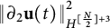
 $$ \begin{align} &\left\lVert \partial_2 \mathbf{u} \right\rVert_{H^{ [\frac{N}{2}] +3}}^2-\frac{d}{dt}\sum_{0\le s\le { [\frac{N}{2}] +3}}\int_{\mathbb{T} ^2}{\Lambda^s} \mathbf{H} \cdot{\Lambda^s}\partial_2 \mathbf{u} \,dx\nonumber\\ &\quad\le C\delta^2\left\lVert a \right\rVert_{H^{ [\frac{N}{2}] +4}}^2+ C\left\lVert \nabla \mathbf{H} \right\rVert_{H^{ [\frac{N}{2}] +4}}^2+C\left\lVert \text{div}\, \mathbf{u} \right\rVert_{H^{ [\frac{N}{2}] +4}}^2, \end{align} $$
which yields the time integrability of
 $\left \lVert \partial _2 \mathbf {u} (t) \right \rVert _{H^{ [\frac {N}{2}] +3}}^2$
. Combining with the generalized Poincaré type inequality induced by Lemma 2.3, we are then able to control the time integrability of low-order Sobolev norms of
 $ \mathbf {u} $
.
The third main step is to establish the stabilizing property of the quantity a. The idea is to make use of the interaction between the equation of
 $a $
and that of
 $\mathbb Q \mathbf {u} $
:
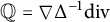
 $$ \begin{align} \begin{cases} \partial_t a+ \text{ div}\, \mathbf{u} =f_1,\\ \partial_t {\mathbb{Q}} \mathbf{u} -\nu\Delta {\mathbb{Q}} \mathbf{u} +\nabla (a + \mathbf{H} _2)={\mathbb{Q}} f_2, \end{cases} \end{align} $$
where
 $\mathbb Q= \nabla \Delta ^{-1} \mbox {div}$
projects vectors onto their gradient parts. Noting that
 ${\mbox {div} {\mathbb {Q}} \mathbf {u} = \text { div}\, \mathbf {u} }$
, we observe that (1.14) involves a wave structure for a and
 ${\mathbb {Q}} \mathbf {u} $
 $$ \begin{align*}\begin{cases} \partial_{tt} a- \nu \Delta \partial_t a-\Delta a =\Delta \mathbf{H} _2, \\ \partial_{tt} {\mathbb{Q}} \mathbf{u} -\nu \Delta \partial_t {\mathbb{Q}} \mathbf{u} -\nabla \mathbf{u} =-\partial_t\Delta \mathbf{H} _2 \end{cases} \end{align*} $$
if neglecting some nonlinear terms. Alternatively, we can introduce the effective velocity by
 $$ \begin{align*} \mathbf{G} \stackrel{\mathrm{def}}{=}{\mathbb{Q}} \mathbf{u} -\frac1\nu\Delta^{-1}\nabla {a}. \end{align*} $$
The effective velocity
 $ \mathbf {G} $
then satisfies the following system:
 $$ \begin{align*} \left\{\begin{aligned} &\partial_t a +\frac1\nu{a}+ \text{ div}\, \mathbf{G} =f_1,\\ &\partial_t \mathbf{G} -\nu\Delta \mathbf{G} =\frac1\nu{\mathbb{Q}} \mathbf{u} -\nabla \mathbf{H} _2 +{\mathbb{Q}} f_2-\frac1\nu\Delta^{-1}\nabla f_1. \end{aligned}\right. \end{align*} $$
These equations clearly reveal the damping in a and the dissipation in
 $ \mathbf {G} $
. We then estimate the Sobolev norms
 $\|a\|_{H^{ [\frac {N}{2}] +4}}$
and
 $\| \mathbf {G} \|_{H^{ [\frac {N}{2}] +4}}$
. Combining (1.12) with
 $\ell = [\frac {N}{2}] +4$
and (1.13) in the previous steps, we then obtain a self-contained inequality.
The last step is to establish (1.11) and close the bootstrapping argument. The energy inequality obtained in the previous steps, together with interpolation inequalities, allows us to show that
 $$ \begin{align} \|(a, \mathbf{u} , \mathbf{H} )(t)\|_{H^{ [\frac{N}{2}] +4}} \le C\, (1+ t)^{-\frac32}, \end{align} $$
In particular, the time integral of
 $\mathrm {Y}^{(\ell )}_{\infty }(t)$
in (1.12) is time integrable:
 $$ \begin{align*}\int_0^\infty \mathrm{Y}^{(\ell)}_{\infty}(t) \,dt \le C <\infty. \end{align*} $$
Grönwall’s inequality then yields
 $$ \begin{align*}\|(a, \mathbf{u} , \mathbf{H} )(t)\|_{H^N} \le C\, \|(a_0, \mathbf{u} _0, \mathbf{H} _0)\|_{H^N}. \end{align*} $$
Taking the initial norm to be sufficiently small, we achieve (1.11). The decay rate in (1.9) is a consequence of (1.15) and an interpolation inequality.
2 Preliminaries
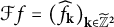
We first denote by
 $\mathcal {F}f=({\widehat{f}}_{\mathbf {k}} )_{\mathbf {k} \in {\widetilde{\mathbb {Z}}}^2}$
the Fourier series of a distribution
 $f\in S'( \mathbb {T} ^2) $
so that
 $$ \begin{align*}f=\sum_{\mathbf{k} \in\widetilde{{\mathbb{Z}}}^2}\widehat{f}_{\mathbf{k}} \frac{e^{i \mathbf{k} \cdot \mathbf{x}}}{\sqrt{| \mathbb{T} ^2|}}, \end{align*} $$
where
 $\widetilde{{\mathbb {Z}}}^2={\mathbb {Z}}/a_1\times {\mathbb {Z}}/a_2$
and
 $| \mathbb {T} ^2|$
stands for the measure of
 $ \mathbb {T} ^2.$
The Sobolev space
 $H^s( \mathbb {T} ^2)$
is defined as follows:
 $$ \begin{align*} H^s( \mathbb{T} ^2)\stackrel{\mathrm{def}}{=}\left\{f\in S'( \mathbb{T} ^2)\Big| \|f\|_{H^s}\stackrel{\mathrm{def}}{=}\Big(|\widehat{f}_0|^2+\sum_{\mathbf{k} \neq0}| \mathbf{k} |^{2s}|\widehat{f}_{\mathbf{k}} |^2\Big)^{\frac12}<\infty \right\}. \end{align*} $$
Next, we present several functional inequalities to be used in the proof of our main result. We first recall a weighted Poincaré inequality first established by Desvillettes and Villani in [Reference Desvillettes and Villani9, p. 288].
Lemma 2.1 Let
 $\Omega $
be a bounded connected Lipschitz domain and
 $\bar {\varrho }$
be a positive constant. There exists a positive constant C, depending on
 $\Omega $
and
 $\bar {\varrho }$
, such that for any nonnegative function
 $\varrho $
satisfying
 $$ \begin{align*} \int_{\Omega}\varrho dx=1, \quad \varrho\le\bar{\varrho}, \end{align*} $$
and any
 $ \mathbf {u} \in H^1(\Omega )$
, there holds
 $$ \begin{align} \int_{\Omega}\varrho \left| \mathbf{u} -\int_{\Omega}\rho \mathbf{u} dx\right|^2dx\le C\|\nabla \mathbf{u} \|_{L^2}^2. \end{align} $$
Although a proof of this lemma can be found in [Reference Desvillettes and Villani9, p. 288], we include it here for the convenience of the reader.
Proof of Lemma 2.1
Let
 $$ \begin{align*} \bar{\mathbf{u}} := \frac{1}{|\Omega|}\int_{\Omega}\mathbf{u}\,dx, \qquad \bar{\mathbf{u}}_{\varrho} := \int_{\Omega}\varrho \mathbf{u}\,dx. \end{align*} $$
By the classical Poincaré inequality, there exists a constant
 $C_P=C_P(\Omega )>0$
such that
 $$ \begin{align} \int_{\Omega}|\mathbf{u}-\bar{\mathbf{u}}|^2\,dx \le C_P\|\nabla \mathbf{u}\|_{L^2(\Omega)}^2. \end{align} $$
We write
 $$ \begin{align*} \mathbf{u}-\bar{\mathbf{u}}_{\varrho} = (\mathbf{u}-\bar{\mathbf{u}}) + (\bar{\mathbf{u}}-\bar{\mathbf{u}}_{\varrho}). \end{align*} $$
Hence,
 $$ \begin{align*} \int_{\Omega}\varrho |\mathbf{u}-\bar{\mathbf{u}}_{\varrho}|^2\,dx =& \int_{\Omega}\varrho |\mathbf{u}-\bar{\mathbf{u}}|^2\,dx\nonumber\\ &+ 2(\bar{\mathbf{u}}-\bar{\mathbf{u}}_{\varrho})\cdot \int_{\Omega}\varrho(\mathbf{u}-\bar{\mathbf{u}})\,dx + |\bar{\mathbf{u}}-\bar{\mathbf{u}}_{\varrho}|^2\int_{\Omega}\varrho\,dx. \end{align*} $$
Using
 $$ \begin{align*} \int_{\Omega}\varrho(\mathbf{u}-\bar{\mathbf{u}})\,dx = \bar{\mathbf{u}}_{\varrho}-\bar{\mathbf{u}}, \qquad \int_{\Omega}\varrho\,dx=1, \end{align*} $$
we obtain
 $$ \begin{align*} \int_{\Omega}\varrho |\mathbf{u}-\bar{\mathbf{u}}_{\varrho}|^2\,dx = \int_{\Omega}\varrho |\mathbf{u}-\bar{\mathbf{u}}|^2\,dx - |\bar{\mathbf{u}}-\bar{\mathbf{u}}_{\varrho}|^2 \le \int_{\Omega}\varrho |\mathbf{u}-\bar{\mathbf{u}}|^2\,dx. \end{align*} $$
Using the bound
 $\varrho \le \bar {\varrho }$
, we further deduce
 $$ \begin{align*} \int_{\Omega}\varrho |\mathbf{u}-\bar{\mathbf{u}}_{\varrho}|^2\,dx \le \bar{\varrho}\int_{\Omega}|\mathbf{u}-\bar{\mathbf{u}}|^2\,dx. \end{align*} $$
Combining this with (2.2) yields
 $$ \begin{align*} \int_{\Omega}\varrho \left|\mathbf{u}-\int_{\Omega}\varrho \mathbf{u}\,dx\right|^2dx \le \bar{\varrho}\, C_P \|\nabla \mathbf{u}\|_{L^2(\Omega)}^2. \end{align*} $$
Thus, (2.1) holds with
 $$ \begin{align*} C=\bar{\varrho}\,C_P. \end{align*} $$
This completes the proof.
In order to remove the weight function
 $\varrho $
in (2.1) without resorting to the lower bound of
 $\varrho $
, we need another variant of Poincaré inequality (see Lemma 3.2 in [Reference Feireisl13]).
Lemma 2.2 Let
 $\Omega $
be a bounded connected Lipschitz domain in
 $\mathbb {R}^2$
and
 $p>1$
be a constant. Given positive constants
 $M_0$
and
 $E_0$
, there is a constant
 $C=C(E_0,M_0)$
such that for any nonnegative function
 $\varrho $
satisfying
 $$ \begin{align*}M_0\leq\int_{\Omega}\varrho dx\quad\mbox{and}\quad \int_{\Omega}\varrho^{p}dx\leq E_0, \end{align*} $$
and for any
 $ \mathbf {u} \in H^1(\Omega )$
, there holds
 $$ \begin{align*}\| \mathbf{u} \|_{L^2}^2\leq C\left[\|\nabla \mathbf{u} \|_{L^2}^2+\left(\int_{\Omega}\varrho| \mathbf{u} |dx\right)^2\right]. \end{align*} $$
Next, we introduce a lemma which plays an important role in capturing the dissipation of the velocity in
 $ \mathbb {T} ^2$
.
Lemma 2.3 Assume that
 $ \mathbf {u} (x) \in H^{k+2}(\mathbb {T}^2)$
with
 $k \in \mathbb {N}$
satisfies the following condition:
 $$ \begin{align} \begin{aligned} \mathbf{u} _1(x) &\quad \text{is even periodic with respect to } x_2,\\ \mathbf{u} _2(x)&\quad \text{is odd periodic with respect to } x_2. \end{aligned} \end{align} $$
Then
 $$ \begin{align*} \|\nabla \mathbf{u} \|_{H^k (\mathbb{T}^2)} \lesssim \|\partial_2 \mathbf{u} \|_{H^{k+1} (\mathbb{T}^2)}+\| \mathrm{div}\, \mathbf{u} \|_{H^k (\mathbb{T}^2)}. \end{align*} $$
Proof This lemma follows essentially from Proposition 2.1 of [Reference Zhou and Zhu45], under the condition that
 $ \text { div}\, \mathbf {u} =0$
. In two dimensions, the vorticity is defined as
 $\omega = \partial _1 \mathbf {u} _2 - \partial _2 \mathbf {u} _1$
. Then the velocity Laplacian decomposes as
 $$ \begin{align*}\Delta \mathbf{u} =\nabla^{\perp}\omega+\nabla \text{ div}\, \mathbf{u} ,\end{align*} $$
where
 $\nabla ^\perp = (-\partial _2, \partial _1)$
. A straightforward computation gives
 $$ \begin{align*}\nabla \mathbf{u} = -\nabla (-\Delta)^{-1}\nabla^{\perp}\omega-\nabla (-\Delta)^{-1} \nabla \text{ div}\, \mathbf{u} .\end{align*} $$
By the standard Calderon–Zygmund theory, the Riesz transform Z satisfies
 $\|Zg\|_{L^p} \lesssim \|g\|_{L^p}$
for
 $1 < p < \infty $
, which implies the estimate
 $$ \begin{align} \|\nabla \mathbf{u} \|_{H^{k}} \lesssim \|\omega\|_{H^{k}}+\| \text{div}\, \mathbf{u} \|_{H^{k}}. \end{align} $$
On the other hand, due to the definition of
 $\omega $
and the assumption (2.3), we easily know that
 $\omega $
is odd periodic with respect to
 $x_2$
which implies
 $$ \begin{align} \frac{1}{2\pi}\int_{-\pi}^{\pi} \omega(x_1,x_2) dx_2 =0, \quad \forall x_1 \in [-\pi,\pi]. \end{align} $$
For a multi-index
 $\alpha = (\alpha _1, \alpha _2)$
, where
 $\partial ^{\alpha } = \partial _1^{\alpha _1}\partial _2^{\alpha _2}$
, we can write
 $$ \begin{align} \|\omega\|^2_{H^k (\mathbb{T}^2)} =\sum_{|\alpha|=0}^k \int_{-\pi}^{\pi} \int_{-\pi}^{\pi} |\partial^{\alpha}\omega(x_1,x_2)|^2 dx_2 dx_1. \end{align} $$
Noting the fact (2.5), we have, for multi-index
 $\alpha =(\alpha _1,0),$
 $$ \begin{align*} \frac{1}{2\pi}\int_{-\pi}^{\pi} \partial^{\alpha}\omega(x_1,x_2) dx_2 =0. \end{align*} $$
Also, for multi-index
 $\alpha =(\alpha _1,\alpha _2)$
with
 $\alpha _2>0$
, using the periodic boundary condition, we have
 $$ \begin{align*} \int_{-\pi}^{\pi} \partial^{\alpha}\omega(x_1,x_2) dx_2 = \partial_1^{\alpha_1}\partial_2^{\alpha_2-1} \omega(x_1,\cdot)\Big|_{-\pi}^{\pi} =0. \end{align*} $$
Therefore, the integral average of
 $\partial ^{\alpha } \omega (x_1, x_2)$
in
 $x_2$
direction over
 $[-\pi , \pi ]$
is zero. Hence, applying standard Poincaré inequality to
 $\partial ^{\alpha }\omega (x_1,x_2)$
in
 $x_2$
direction, we have
 $\forall x_1 \in [-\pi ,\pi ]$
:
 $$ \begin{align*} \int_{-\pi}^{\pi} |\partial^{\alpha}\omega(x_1,x_2)|^2 dx_2 \lesssim \int_{-\pi}^{\pi} |\partial^{\alpha}\partial_2\omega(x_1,x_2)|^2 dx_2. \end{align*} $$
According to the definition of
 $\|\omega \|_{H^k(\mathbb {T}^2)}$
, that is, (2.6), we finally obtain
 $$ \begin{align} \begin{aligned} \|\omega\|^2_{H^k (\mathbb{T}^2)} &=\sum_{|\alpha|=0}^k \int_{-\pi}^{\pi} \int_{-\pi}^{\pi} |\partial^{\alpha}\omega(x_1,x_2)|^2 dx_2 dx_1 \\&\lesssim \sum_{|\alpha|=0}^k \int_{-\pi}^{\pi} \int_{-\pi}^{\pi} |\partial^{\alpha}\partial_2\omega(x_1,x_2)|^2 dx_2 dx_1 \\&= \|\partial_2\omega\|^2_{H^k (\mathbb{T}^2)}. \end{aligned} \end{align} $$
Inserting (2.7) into (2.4), we get
 $$ \begin{align*} \|\nabla \mathbf{u} \|_{H^{k}(\mathbb{T}^2)} \lesssim& \|\partial_2 \omega\|_{H^{k}(\mathbb{T}^2)}+\| \text{div}\, \mathbf{u} \|_{H^{k}}\nonumber\\ \lesssim& \|\partial_2 \mathbf{u} \|_{H^{k+1}(\mathbb{T}^2)}+\| \text{div}\, \mathbf{u} \|_{H^{k}}. \end{align*} $$
This finishes the proof.
Finally, we recall several calculus inequalities.
Lemma 2.4 (Gagliardo–Nirenberg’s inequality in
$\mathbb { \mathbb {T} }^2$
[Reference Nirenberg31])

Let
 $0 \leq m$
,
 $s \leq \kappa $
, then we have
 $$ \begin{align*} \|\Lambda^s f\|_{L^p}\le C \|\Lambda^mf\|_{L^q}^{1-\theta}\|\Lambda^{\kappa}f\|_{L^r}^\theta, \end{align*} $$
where
 $\theta \in [0, 1]$
and
 $\theta $
satisfies
 $ \frac {s}{2}-\frac {1}{p}=\big (\frac {m}{2} -\frac {1}{q}\big )(1-\theta ) +\left (\frac {\kappa }{2}-\frac {1}{r}\right ) \theta $
. When
 $p = \infty $
, we require that
 $0 < \theta < 1$
.
Lemma 2.5 (Kato–Ponce product estimate [Reference Grafakos and Oh16, Reference Kato and Ponce22])
For any
 $s>0$
,
 $1<p<\infty $
,
 $1< q_1, q_2< \infty ,$
and
 $1< p_1, p_2\leq \infty $
, we have
 $$ \begin{align*} \|\Lambda^s(fg)\|_{L^p} \leq C\big(\|f\|_{L^{p_1}} \|\Lambda^s g\|_{L^{q_1}} + \|g\|_{L^{p_2}}\|\Lambda^s f\|_{L^{q_2}} \big), \end{align*} $$
where
 $\frac {1}{p} = \frac {1}{p_1} + \frac {1}{q_1} = \frac {1}{p_2} + \frac {1}{q_2}$
.
Lemma 2.6 (Commutator estimate [Reference Kato and Ponce22])
Let
 $s> 0$
. Then there exists a constant C such that, for any
 $f\in {H^{s}}( \mathbb {T} ^2)\cap W^{1,\infty }( \mathbb {T} ^2)$
,
 $g\in {H^{s-1}}( \mathbb {T} ^2)\cap {L^\infty }( \mathbb {T} ^2)$
, there holds
 $$ \begin{align*} \big\|[ \Lambda ^s,f\cdot\nabla ]g\big\|_{L^2}\le C(\left\lVert \nabla f \right\rVert_{L^\infty}\left\lVert \Lambda ^sg \right\rVert_{L^2}+\left\lVert \Lambda ^s f \right\rVert_{L^2}\left\lVert \nabla g \right\rVert_{L^\infty}). \end{align*} $$
Lemma 2.7 [Reference Triebel36]
Let
 $s>0$
and
 $f\in H^s( \mathbb {T} ^2)\cap L^\infty ( \mathbb {T} ^2)$
. Assume that F is a smooth function on
 ${\mathbb {R}}$
with
 $F(0)=0$
. Then we have
 $$ \begin{align*}\|F(f)\|_{H^s}\le C(1+\|f\|_{L^\infty})^{[s]+1}\|f\|_{H^s}, \end{align*} $$
where the constant C depends on
 $\sup _{k\le {[s]+2},t\le \|f\|_{L^\infty }} \|F^{(k)}(t)\|_{L^\infty }.$
3 Proof of Theorem 1.1
Given the initial data
 $(\rho _0, \mathbf {u} _0, \mathbf {B} _0-\mathbf {e}_2)\in H^{N}( \mathbb {T} ^2)$
, the local well-posedness of the system (1.10) could be proven by using the standard energy method (see, e.g., [Reference Kawashima23]). Thus, we may assume that there exists
 $T> 0$
such that the system (1.10) has a unique solution
 $(\rho -\bar {\rho }, \mathbf {u} , \mathbf {B} -\mathbf {e}_2)\in C([0,T];H^{N})$
. Moreover,
 $$ \begin{align} \frac12c_0\le\rho(t,x)\le 2c_0^{-1},\quad\text{for any } {t\in[0,T]}. \end{align} $$
We use the bootstrapping argument to show that this local solution can be extended into a global one. The goal is to derive a global a priori upper bound. To initiate the bootstrapping argument, we make the ansatz that
 $$ \begin{align*} \sup_{t\in[0,T]}(\left\lVert \rho-\bar{\rho} \right\rVert_{H^{N}}+\left\lVert \mathbf{u} \right\rVert_{H^{N}}+\left\lVert \mathbf{B} -\mathbf{e}_2 \right\rVert_{H^{N}})\le \delta, \end{align*} $$
where
 $0<\delta <1$
obeys requirements to be specified later. In the following sections, we prove that if the initial norm is taken to be sufficiently small, namely,
 $$ \begin{align*}\|\rho_0- \bar\rho\|_{H^N} +\| \mathbf{u} _0\|_{H^N}+\| \mathbf{B} _0-\mathbf{e}_2\|_{H^N}\le \varepsilon, \end{align*} $$
with sufficiently small
 $\varepsilon>0$
, then
 $$ \begin{align*}\sup_{t\in[0,T]}(\left\lVert \rho-\bar{\rho} \right\rVert_{H^{N}}+\left\lVert \mathbf{u} \right\rVert_{H^{N}}+\left\lVert \mathbf{B} -\mathbf{e}_2 \right\rVert_{H^{N}})\le \frac{\delta}{2}. \end{align*} $$
The bootstrapping argument then leads to the desired global bound. To arrive at our aim, we denote
 $\bar \rho =1$
and
 $$ \begin{align*}\mathbf{B}_0= \mathbf{H} _0 + \mathbf{e}_2,\quad\text{with}\quad\mathbf{e}_2=(0,1)^{\top},\end{align*} $$
from which there holds
 $$ \begin{align*} \int_{\mathbb{T}^2} \mathbf{H} _0 \,dx = 0. \end{align*} $$
Define
 $$ \begin{align*} a=\rho-1,\quad \mathbf{H} = \mathbf{B} -\mathbf{e}_2, \end{align*} $$
and
 $$ \begin{align*}I(a)\stackrel{\mathrm{def}}{=}\frac{a}{1+a},\quad k(a)\stackrel{\mathrm{def}}{=}\frac{P'(1+a)}{1+a}-1.\end{align*} $$
Then system (1.1) can be reformulated as
 $$ \begin{align} \left\{\begin{aligned} &\partial_t a+ \text{div}\, \mathbf{u} ={f}_1,\\ &\partial_t \mathbf{u} -{\nu}\nabla \text{div}\, \mathbf{u} +\nabla a =\partial_2 \mathbf{H} -\nabla \mathbf{H} _2+{f}_2,\\ &\partial_t \mathbf{H} -\sigma\Delta \mathbf{H} =\partial_2 \mathbf{u} -\mathbf{e}_2 \text{div}\, \mathbf{u} +{f}_3,\\ & \text{ div}\, \mathbf{H} =0,\\ &(a, \mathbf{u} , \mathbf{H} )|_{t=0}=(a_0, \mathbf{u} _0, \mathbf{H} _0), \end{aligned}\right. \end{align} $$
where
 $$ \begin{align*} {f}_1\stackrel{\mathrm{def}}{=}&- \mathbf{u} \cdot\nabla a-a \text{ div}\, \mathbf{u} ,\nonumber\\ {f}_2\stackrel{\mathrm{def}}{=}&- \mathbf{u} \cdot\nabla \mathbf{u} + \mathbf{H} \cdot\nabla \mathbf{H} + \mathbf{H} \nabla \mathbf{H} +k(a)\nabla a +\nu I(a)\nabla \text{ div}\, \mathbf{u} \nonumber\\ &-I(a)(\partial_2 \mathbf{H} + \mathbf{H} \cdot\nabla \mathbf{H} -\nabla \mathbf{H} _2- \mathbf{H} \nabla \mathbf{H} ),\nonumber\\ {f}_3\stackrel{\mathrm{def}}{=}&- \mathbf{u} \cdot\nabla \mathbf{H} + \mathbf{H} \cdot\nabla \mathbf{u} - \mathbf{H} \text{ div}\, \mathbf{u}. \end{align*} $$
In what follows, we divide the proof of Theorem 1.1 into six sections.
3.1 Basic energy estimates
Denote by
 $g(\rho )$
the potential energy density, namely,
 $$ \begin{align*} g(\rho)=\rho\int_{\bar{\rho}}^\rho\frac{P(\tau)-P(1)}{\tau^2}\,d\tau. \end{align*} $$
The standard basic energy estimate gives
 $$ \begin{align} \frac12\frac{d}{dt}\int_{\mathbb{T} ^2}\left(2g(\rho)+\rho| \mathbf{u} |^2+| \mathbf{H} |^2\right)\,dx+\nu\left\lVert \text{div}\, \mathbf{u} \right\rVert_{L^2}^2 +\sigma\left\lVert \nabla \mathbf{H} \right\rVert_{L^2}^2=0, \end{align} $$
where we have used the following cancellations:
 $$ \begin{align*} &\int_{\mathbb{T} ^2}(\partial_2 \mathbf{H} + \mathbf{H} \cdot\nabla \mathbf{H} )\cdot \mathbf{u} \,dx+\int_{\mathbb{T} ^2}(\partial_2 \mathbf{u} + \mathbf{H} \cdot\nabla \mathbf{u} )\cdot \mathbf{H} \,dx=0,\nonumber\\ &\int_{\mathbb{T} ^2}( \mathbf{H} \nabla \mathbf{H} +\nabla \mathbf{H} _2)\cdot \mathbf{u} \,dx+\int_{\mathbb{T} ^2}( \mathbf{u} \cdot\nabla \mathbf{H} + \mathbf{e}_2 \text{ div}\, \mathbf{u} + \mathbf{H} \text{ div}\, \mathbf{u} )\cdot \mathbf{H} \,dx=0. \end{align*} $$
For any fixed positive constant
 $c_0$
, if
 $c_0\le \rho \le c_0^{-1}$
, then
 $$ \begin{align*} g(\rho)\sim (\rho-1)^2. \end{align*} $$
Hence, (3.3) implies the result in the following lemma.
Lemma 3.1
 $$ \begin{align} \frac12\frac{d}{dt}\left\lVert (a, \mathbf{u} , \mathbf{H} ) \right\rVert_{L^2}^2+\nu\left\lVert \mathrm{div}\, \mathbf{u} \right\rVert_{L^2}^2+\sigma\left\lVert \nabla \mathbf{H} \right\rVert_{L^2}^2=0. \end{align} $$
In view of Lemmas 2.1 and 2.2 and (1.6), we have the following Poincaré type inequalities, which will be frequently used in this article.
Lemma 3.2 (Poincaré type inequalities)
Let
 $\rho , \mathbf {u} $
, and
 $ \mathbf {H} $
be smooth functions to (1.10) on
 $[0,\infty )\times \mathbb {T}^2$
satisfying (1.6), then for any
 $t\ge 0$
, there hold
 $$ \begin{align} \| \mathbf{H} (t)\|_{L^2}^2\le C\|\nabla \mathbf{H} (t)\|_{L^2}^2, \end{align} $$
 $$ \begin{align} \|(\sqrt{\rho } \mathbf{u} )(t)\|_{L^2}^2\le C\|\nabla \mathbf{u} (t)\|_{L^2}^2, \end{align} $$
and
 $$ \begin{align} \| \mathbf{u} (t)\|_{L^2}^2\le C\|\nabla \mathbf{u} (t)\|_{L^2}^2. \end{align} $$
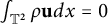
Proof Clearly, due to (1.3), (3.5) is a standard Poincaré inequality. Equation (3.6) follows from Lemma 2.1 and
 $\int _{\mathbb {T}^2}\rho \mathbf {u} dx=0$
in (1.3). Equation (3.7) is a consequence of (3.6) and Lemma 2.2.
Throughout, we make the assumption that
 $$ \begin{align} \sup_{t\in{\mathbb{R}}_+,\, x\in \mathbb{T} ^2} |a(t,x)|\leq \frac12. \end{align} $$
Because of
 $H^2( \mathbb {T} ^2)\hookrightarrow L^\infty ( \mathbb {T} ^2),$
(3.8) is ensured by the fact that the solution constructed here has small norm in
 $H^2( \mathbb {T} ^2)$
. It then follows from Lemma 2.7 that the following composition estimate holds:
 $$ \begin{align} \|F(a)\|_{H^s}\le C\|a\|_{H^s} \quad\text{for any } F(0)=0 \text{ and } s>0. \end{align} $$
3.2 Higher-order energy estimates
This section is devoted to the derivation of higher-order energy estimates. The main result is summarized in the following lemma.
Lemma 3.3 Let
 $(a, \mathbf {u} , \mathbf {H} ) \in C([0, T];H^N)$
be a solution to the system (3.2). For any
 $0\le \ell \le N$
, there holds
 $$ \begin{align} &\frac12\frac{d}{dt}\left\lVert (a, \mathbf{u} , \mathbf{H} ) \right\rVert_{H^{\ell}}^2 +\nu\left\lVert \mathrm{div}\, \mathbf{u} \right\rVert_{H^{\ell}}^2+\sigma\left\lVert \nabla \mathbf{H} \right\rVert_{H^{\ell}}^2\le C \mathrm{Y}^{(\ell)}_{\infty}(t)\left\lVert (a, \mathbf{u} , \mathbf{H} ) \right\rVert_{H^{\ell}}^2 \end{align} $$
with
 $$ \begin{align*} \mathrm{Y}^{(\ell)}_{\infty}(t)\stackrel{\mathrm{def}}{=}& \left\lVert (\nabla a,\nabla \mathbf{u} ,\nabla\ \mathrm{div}\, \mathbf{u} ,\nabla \mathbf{H} ) \right\rVert_{L^\infty}+\left\lVert a \right\rVert_{H^{[\frac{\ell-1}{2}]+4}} +\left\lVert a \right\rVert_{H^{\ell-[\frac{\ell-1}{2}]}} \notag\\&+\left\lVert \mathrm{div}\, \mathbf{u} \right\rVert_{H^{\ell-[\frac{\ell-1}{2}]}}+\left\lVert a \right\rVert_{H^{[\frac{\ell-1}{2}]+3}}^2 +\left\lVert (\nabla a,\nabla \mathbf{u} ,\nabla \mathbf{H} ) \right\rVert_{L^\infty}^2 \notag\\ &+\|(a, \mathbf{H} )\|_{L^{\infty}}^2 +\|a\|_{L^{\infty}}^2\| \mathbf{H} \|_{L^{\infty}}^2+\| \mathbf{H} \|_{L^{\infty}}^2\|\nabla \mathbf{H} \|_{L^{\infty}}^2. \end{align*} $$
Proof Equation (3.10) with
 $\ell =0$
is the basic energy inequality in Lemma 3.1. We consider the case when
 $\ell \ge 1$
. Writing
 $\Lambda =\sqrt {-\Delta }$
and applying
 $ \Lambda ^s$
with
 $1\le s\le \ell $
to (3.2) and then taking
 $L^2$
inner product with
 $( \Lambda ^sa, \Lambda ^s \mathbf {u} , \Lambda ^s \mathbf {H} )$
yields
 $$ \begin{align} &\frac12\frac{d}{dt}\left\lVert ( \Lambda ^sa, \Lambda ^s \mathbf{u} , \Lambda ^s \mathbf{H} ) \right\rVert_{L^2}^2 -\int_{\mathbb{T} ^2} \Lambda ^{s}\nabla(\bar{\nu}(\rho) \text{ div}\, \mathbf{u} )\cdot \Lambda ^{s} \mathbf{u} \,dx+\sigma\left\lVert \Lambda ^s\nabla \mathbf{H} \right\rVert_{L^2}^2 \nonumber\\ &\quad= \int_{\mathbb{T} ^2} \Lambda ^{s} f_1\cdot \Lambda ^{s} a\,dx+\int_{\mathbb{T} ^2} \Lambda ^{s} f_2\cdot \Lambda ^{s} \mathbf{u} \,dx+\int_{\mathbb{T} ^2} \Lambda ^{s} f_3\cdot \Lambda ^{s} \mathbf{H} \,dx, \end{align} $$
where we have used the following cancellations:
 $$ \begin{align*} &\int_{\mathbb{T} ^2} \Lambda ^s \text{ div}\, \mathbf{u} \cdot \Lambda ^s a\,dx+\int_{\mathbb{T} ^2} \Lambda ^s \nabla a\cdot \Lambda ^s \mathbf{u} \,dx=0;\nonumber\\ &\int_{\mathbb{T} ^2} \Lambda ^s\partial_2 \mathbf{H} \cdot \Lambda ^s \mathbf{u} \,dx+\int_{\mathbb{T} ^2} \Lambda ^s \partial_2 \mathbf{u} \cdot \Lambda ^s \mathbf{H} \,dx=0;\nonumber\\ &\int_{\mathbb{T} ^2} \Lambda ^s\nabla \mathbf{H} _2\cdot \Lambda ^s \mathbf{u} \,dx+\int_{\mathbb{T} ^2} \Lambda ^s ( \mathbf{e}_2 \text{ div}\, \mathbf{u} )\cdot \Lambda ^s \mathbf{H} \,dx=0. \end{align*} $$
The second term on the left-hand side can be written as
 $$ \begin{align} -\int_{\mathbb{T} ^2} \Lambda ^{s}\nabla(\bar{\nu}(\rho) \text{ div}\, \mathbf{u} )\cdot \Lambda ^{s} \mathbf{u} \,dx =&\int_{\mathbb{T} ^2} \Lambda ^{s}(\bar{\nu}(\rho) \text{ div}\, \mathbf{u} )\cdot \Lambda ^{s} \text{ div}\, \mathbf{u} \,dx\nonumber\\ =& \int_{\mathbb{T} ^2}\bar{\nu}(\rho) \Lambda ^{s} \text{ div}\, \mathbf{u} \cdot \Lambda ^{s} \text{ div}\, \mathbf{u} \,dx\nonumber\\ &+\int_{\mathbb{T} ^2}[ \Lambda ^{s},\bar{\nu}(\rho)] \text{ div}\, \mathbf{u} \cdot \Lambda ^{s} \text{ div}\, \mathbf{u} \,dx. \end{align} $$
Due to (3.1), we have for any
 $t\in [0,T]$
that
 $$ \begin{align} \int_{\mathbb{T} ^2}\bar{\nu}(\rho) \Lambda ^{s} \text{ div}\, \mathbf{u} \cdot \Lambda ^{s} \text{ div}\, \mathbf{u} \,dx\ge c_0^{-1}\nu\left\lVert \Lambda ^{s} \text{ div}\, \mathbf{u} \right\rVert_{L^{2}}^2. \end{align} $$
For the last term in (3.12), we first rewrite this term into
 $$ \begin{align*} \int_{\mathbb{T} ^2}[ \Lambda ^{s},\bar{\nu}(\rho)] \text{ div}\, \mathbf{u} \cdot \Lambda ^{s} \text{ div}\, \mathbf{u} \,dx =&\int_{\mathbb{T} ^2}[ \Lambda ^{s},\bar{\nu}(\rho)-\nu+\nu] \text{ div}\, \mathbf{u} \cdot \Lambda ^{s} \text{ div}\, \mathbf{u} \,dx\nonumber\\ =&-\int_{\mathbb{T} ^2}[ \Lambda ^{s},\nu I(a)] \text{ div}\, \mathbf{u} \cdot \Lambda ^{s} \text{ div}\, \mathbf{u} \,dx. \end{align*} $$
Then, with the aid of Lemmas 2.6 and 2.7 and (3.9), we have
 $$ \begin{align} &\Big|\int_{\mathbb{T} ^2}[ \Lambda ^{s},\nu I(a)] \text{ div}\, \mathbf{u} \cdot \Lambda ^{s} \text{ div}\, \mathbf{u} \,dx\Big| \nonumber\\ &\quad \le C\left\lVert \Lambda ^{s} \text{ div}\, \mathbf{u} \right\rVert_{L^{2}}(\left\lVert \nabla I(a) \right\rVert_{L^\infty}\left\lVert \Lambda ^{s} \mathbf{u} \right\rVert_{L^2}+\left\lVert \nabla \mathbf{u} \right\rVert_{L^\infty}\left\lVert \Lambda ^{s}I(a) \right\rVert_{L^2})\nonumber\\ &\quad \le \frac{c_0^{-1}}{2}\nu\left\lVert \Lambda ^{s} \text{ div}\, \mathbf{u} \right\rVert_{L^{2}}^2+C(\left\lVert \nabla a \right\rVert_{L^\infty}^2\left\lVert \Lambda ^{s} \mathbf{u} \right\rVert_{L^2}^2+\left\lVert \nabla \mathbf{u} \right\rVert_{L^\infty}^2\left\lVert \Lambda ^{s}a \right\rVert_{L^2}^2). \end{align} $$
Inserting (3.13) and (3.14) into (3.12) leads to
 $$ \begin{align*} -\int_{\mathbb{T} ^2} \Lambda ^{s}\nabla(\bar{\nu}(\rho) \text{ div}\, \mathbf{u} )\cdot \Lambda ^{s} \mathbf{u} \,dx \ge&\frac{c_0^{-1}}{2}\nu\left\lVert \Lambda ^{s} \text{ div}\, \mathbf{u} \right\rVert_{L^{2}}^2\nonumber\\ &-C(\left\lVert \nabla a \right\rVert_{L^\infty}^2\left\lVert \Lambda ^{s} \mathbf{u} \right\rVert_{L^2}^2+\left\lVert \nabla \mathbf{u} \right\rVert_{L^\infty}^2\left\lVert \Lambda ^{s}a \right\rVert_{L^2}^2). \end{align*} $$
Hence,
 $$ \begin{align} &\frac12\frac{d}{dt}\left\lVert ( \Lambda ^sa, \Lambda ^s \mathbf{u} , \Lambda ^s \mathbf{H} ) \right\rVert_{L^2}^2 +{c_0^{-1}}\nu\left\lVert \Lambda ^{s}\mbox{div} \mathbf{u} \right\rVert_{L^2}^2 +\sigma\left\lVert \Lambda ^s\nabla \mathbf{H} \right\rVert_{L^2}^2\nonumber\\ &\quad\le C(\left\lVert \nabla a \right\rVert_{L^\infty}^2\left\lVert \Lambda ^{s} \mathbf{u} \right\rVert_{L^2}^2+\left\lVert \nabla \mathbf{u} \right\rVert_{L^\infty}^2\left\lVert \Lambda ^{s}a \right\rVert_{L^2}^2)\nonumber\\ &\qquad+ \int_{\mathbb{T} ^2} \Lambda ^{s} f_1\cdot \Lambda ^{s} a\,dx+\int_{\mathbb{T} ^2} \Lambda ^{s} f_2\cdot \Lambda ^{s} \mathbf{u} \,dx+\int_{\mathbb{T} ^2} \Lambda ^{s} f_3\cdot \Lambda ^{s} \mathbf{H} \,dx. \end{align} $$
Summing (3.15) over
 $1\le s\le \ell $
and then adding to (3.4) gives
 $$ \begin{align} &\frac12\frac{d}{dt}\left\lVert (a, \mathbf{u} , \mathbf{H} ) \right\rVert_{H^{\ell}}^2 +{c_0^{-1}}\nu\left\lVert \text{div}\, \mathbf{u} \right\rVert_{H^{\ell}}^2+\sigma\left\lVert \nabla \mathbf{H} \right\rVert_{H^{\ell}}^2\nonumber\\ &\quad\le C\left\lVert (\nabla a, \nabla \mathbf{u} ) \right\rVert_{L^\infty}^2\left\lVert (a, \mathbf{u} ) \right\rVert_{H^{\ell}}^2+\sum_{s=1}^{\ell} \int_{\mathbb{T} ^2} \Lambda ^{s} f_1\cdot \Lambda ^{s} a\,dx\nonumber\\ &\qquad+\sum_{s=1}^{\ell}\int_{\mathbb{T} ^2} \Lambda ^{s} f_2\cdot \Lambda ^{s} \mathbf{u} \,dx+\sum_{s=1}^{\ell}\int_{\mathbb{T} ^2} \Lambda ^{s} f_3\cdot \Lambda ^{s} \mathbf{H} \,dx. \end{align} $$
We now estimate successively terms on the right-hand side of (3.16). To bound the first term in
 $f_1$
, we rewrite it into
 $$ \begin{align} &\sum_{s=1}^{\ell}\int_{\mathbb{T} ^2} \Lambda ^{s} ( \mathbf{u} \cdot\nabla a)\cdot \Lambda ^{s} a\,dx\nonumber\\ &\quad=\sum_{s=1}^{\ell}\int_{\mathbb{T} ^2}( \Lambda ^{s} ( \mathbf{u} \cdot\nabla a)- \mathbf{u} \cdot\nabla \Lambda ^{s}a)\cdot \Lambda ^{s} a\,dx +\sum_{s=1}^{\ell}\int_{\mathbb{T} ^2} \mathbf{u} \cdot\nabla \Lambda ^{s}a\cdot \Lambda ^{s} a\,dx\nonumber\\ &\quad\stackrel{\mathrm{def}}{=}A_1+A_2. \end{align} $$
It follows from Lemma 2.6 that
 $$ \begin{align} A_1& \le\, C\sum_{s=1}^{\ell}\left\lVert [ \Lambda ^s, \mathbf{u} \cdot\nabla ]a \right\rVert_{L^2}\left\lVert \Lambda ^{s}a \right\rVert_{L^2}\nonumber\\ & \le\, C\sum_{s=1}^{\ell}(\left\lVert \nabla \mathbf{u} \right\rVert_{L^\infty}\left\lVert \Lambda ^{s}a \right\rVert_{L^2}+\left\lVert \Lambda ^{s} \mathbf{u} \right\rVert_{L^2}\left\lVert \nabla a \right\rVert_{L^\infty})\left\lVert \Lambda ^{s}a \right\rVert_{L^2}\nonumber\\ & \le\, C\left\lVert (\nabla a,\nabla \mathbf{u} ) \right\rVert_{L^\infty}\left\lVert (a, \mathbf{u} ) \right\rVert_{H^{\ell}}^2. \end{align} $$
By integration by parts, we have
 $$ \begin{align} A_2& \le\, C\sum_{s=1}^{\ell}\left\lVert \nabla \mathbf{u} \right\rVert_{L^\infty}\left\lVert \Lambda ^{s}a \right\rVert_{L^2}^2 \le C\left\lVert \nabla \mathbf{u} \right\rVert_{L^\infty}\left\lVert a \right\rVert_{H^{\ell}}^2. \end{align} $$
For the second term in
 $f_1$
, it follows from Lemma 2.5 that
 $$ \begin{align} &\sum_{s=1}^{\ell}\int_{\mathbb{T} ^2} \Lambda ^{s} (a \text{ div}\, \mathbf{u} )\cdot \Lambda ^{s} a\,dx\nonumber\\ &\quad\leq C\sum_{s=1}^{\ell}\big(\| \text{div}\, \mathbf{u} \|_{L^{\infty}}\| \Lambda ^{s} a\|_{L^{2}} +\| \Lambda ^{s} \text{ div}\, \mathbf{u} \|_{L^{2}}\|a\|_{L^{\infty}}\big)\left\lVert \Lambda ^{s}a \right\rVert_{L^2}\nonumber\\ &\quad \leq\frac{c_0^{-1}\nu}{16}\| \text{div}\, \mathbf{u} \|_{H^{\ell}}^2+C(\|\nabla \mathbf{u} \|_{L^{\infty}}+\|a\|_{L^{\infty}}^2) \left\lVert a \right\rVert_{H^{\ell}}^2. \end{align} $$
Collecting (3.18)–(3.20), we can get
 $$ \begin{align} \Big|\sum_{s=1}^{\ell}\int_{\mathbb{T} ^2} \Lambda ^{s} f_1\cdot \Lambda ^{s} a\,dx\Big| \le&\,\frac{c_0^{-1}\nu}{16}\| \text{div}\, \mathbf{u} \|_{H^{\ell}}^2\nonumber\\ &+C(\left\lVert (\nabla a,\nabla \mathbf{u} ) \right\rVert_{L^\infty}+\|a\|_{L^{\infty}}^2)\left\lVert (a, \mathbf{u} ) \right\rVert_{H^{\ell}}^2. \end{align} $$
For the first term in
 $f_3$
, in a similar way as (3.18) and (3.19), we can deduce that
 $$ \begin{align} \sum_{s=1}^{\ell}\int_{\mathbb{T} ^2} \Lambda ^{s} ( \mathbf{u} \cdot\nabla \mathbf{H} )\cdot \Lambda ^{s} \mathbf{H} \,dx & \le\, C\left\lVert (\nabla \mathbf{u} ,\nabla \mathbf{H} ) \right\rVert_{L^\infty}\left\lVert ( \mathbf{u} , \mathbf{H} ) \right\rVert_{H^{\ell}}^2. \end{align} $$
For the last two terms in
 ${f_3}$
, we get by Lemma 2.5 and the Young inequality that
 $$ \begin{align*} &\sum_{s=1}^{\ell}\int_{\mathbb{T} ^2} \Lambda ^{s} ( \mathbf{H} \cdot\nabla \mathbf{u} - \mathbf{H} \text{ div}\, \mathbf{u} )\cdot \Lambda ^{s} \mathbf{H} \,dx\nonumber\\ &\quad\leq\sum_{s=1}^{\ell}\frac{\sigma}{16}\| \Lambda ^{s}\nabla \mathbf{H} \|_{L^{2}}^2 +C\sum_{s=1}^{\ell}(\|\nabla \mathbf{u} \|_{L^{\infty}}^2+\| \mathbf{H} \|_{L^{\infty}}^2) \left\lVert \Lambda ^{s} \mathbf{H} \right\rVert_{L^2}^2\nonumber\\ &\quad\leq \frac{\sigma}{16}\|\nabla \mathbf{H} \|_{H^{\ell}}^2 +C\|(\nabla \mathbf{u} , \mathbf{H} )\|_{L^{\infty}}^2\| \mathbf{H} \|_{H^{\ell}}^2 \end{align*} $$
from which and (3.22), we can conclude that
 $$ \begin{align} \Big|\sum_{s=1}^{\ell}\int_{\mathbb{T} ^2} \Lambda ^{s} f_3\cdot \Lambda ^{s} \mathbf{H} \,dx\Big| \le&\frac{\sigma}{16}\|\nabla \mathbf{H} \|_{H^{\ell}}^2 \\ &+C(\left\lVert (\nabla \mathbf{u} ,\nabla \mathbf{H} ) \right\rVert_{L^\infty}+\|(\nabla \mathbf{u} , \mathbf{H} )\|_{L^{\infty}}^2)\left\lVert ( \mathbf{u} , \mathbf{H} ) \right\rVert_{H^\ell}^2.\nonumber \end{align} $$
In order to bound the rest terms in
 $f_2$
, we write
 $$ \begin{align} \sum_{s=1}^{\ell}\int_{\mathbb{T} ^2} \Lambda ^{s} f_2\cdot \Lambda ^{s} \mathbf{u} \,dx=\sum_{i=3}^8A_i \end{align} $$
with
 $$ \begin{align*} A_3\stackrel{\mathrm{def}}{=}&\sum_{s=1}^{\ell}\int_{\mathbb{T} ^2} \Lambda ^{s} ( \mathbf{u} \cdot\nabla \mathbf{u} )\cdot \Lambda ^{s} \mathbf{u} \,dx, \nonumber\\ A_4\stackrel{\mathrm{def}}{=}&\sum_{s=1}^{\ell}\int_{\mathbb{T} ^2} \Lambda ^{s} ( \mathbf{H} \cdot\nabla \mathbf{H} - \mathbf{H} \nabla \mathbf{H} )\cdot \Lambda ^{s} \mathbf{u} \,dx,\nonumber\\ A_5\stackrel{\mathrm{def}}{=}&\sum_{s=1}^{\ell}\int_{\mathbb{T} ^2} \Lambda ^{s} (k(a)\nabla a)\cdot \Lambda ^{s} \mathbf{u} \,dx, \nonumber\\ A_6\stackrel{\mathrm{def}}{=}&\sum_{s=1}^{\ell}\int_{\mathbb{T} ^2} \Lambda ^{s}( \nu\nabla I(a) \text{ div}\, \mathbf{u} )\cdot \Lambda ^{s} \mathbf{u} \,dx,\notag\\ A_7\stackrel{\mathrm{def}}{=}&\sum_{s=1}^{\ell}\int_{\mathbb{T} ^2} \Lambda ^{s} (I(a)(\partial_2 \mathbf{H} -\nabla \mathbf{H} _2))\cdot \Lambda ^{s} \mathbf{u} \,dx,\nonumber\\ A_8\stackrel{\mathrm{def}}{=}&\sum_{s=1}^{\ell}\int_{\mathbb{T} ^2} \Lambda ^{s} (I(a)( \mathbf{H} \cdot\nabla \mathbf{H} - \mathbf{H} \nabla \mathbf{H} ))\cdot \Lambda ^{s} \mathbf{u} \,dx. \end{align*} $$
The term
 $A_3$
can be bounded the same as (3.17)
 $$ \begin{align*} A_3\le C\left\lVert \nabla \mathbf{u} \right\rVert_{L^\infty}\left\lVert \mathbf{u} \right\rVert_{H^\ell}^2. \end{align*} $$
We next deal with the term
 $A_4$
. In view of
 $ \text { div}\, \mathbf {H} =0,$
one can write
 $$ \begin{align*} A_4 & \leq \, C\sum_{s=1}^{\ell}(\| \mathbf{H} \|_{L^{\infty}} \left\lVert \Lambda ^{s+1} \mathbf{H} \right\rVert_{L^2}+\|\nabla \mathbf{H} \|_{L^{\infty}} \left\lVert \Lambda ^{s} \mathbf{H} \right\rVert_{L^2})\| \Lambda ^{s} \mathbf{u} \|_{L^{2}}\nonumber\\ & \leq\frac{\sigma}{16}\left\lVert \nabla \mathbf{H} \right\rVert_{H^\ell}^2+C\|(\nabla \mathbf{H} , \mathbf{H} )\|_{L^{\infty}}^2 \|( \mathbf{u} , \mathbf{H} )\|_{H^{\ell}}^2. \end{align*} $$
In view of Lemma 2.5, we have
 $$ \begin{align*} A_7 & \leq C\sum_{s=1}^{\ell}\big(\|I(a)\|_{L^{\infty}}\|\nabla \mathbf{H} \|_{H^{s}} +\|I(a)\|_{H^{s}}\|\nabla \mathbf{H} \|_{L^{\infty}}\big)\left\lVert \Lambda ^{s} \mathbf{u} \right\rVert_{L^2}\nonumber\\ & \leq\frac{\sigma}{16}\left\lVert \nabla \mathbf{H} \right\rVert_{H^\ell}^2+C(\|a\|_{L^{\infty}}^2+\|\nabla \mathbf{H} \|_{L^{\infty}}) \left\lVert (a, \mathbf{u} ) \right\rVert_{H^\ell}^2. \end{align*} $$
For the last term
 $A_8$
, we use Lemmas 2.5 and 2.7 again to get
 $$ \begin{align} A_8 &\leq C\big(\|I(a)\|_{L^{\infty}}\| \mathbf{H} \nabla \mathbf{H} \|_{H^{\ell}} +\|I(a)\|_{H^{\ell}}\| \mathbf{H} \nabla \mathbf{H} \|_{L^{\infty}}\big)\left\lVert \mathbf{u} \right\rVert_{H^\ell}. \end{align} $$
Due to
 $$ \begin{align*} \| \mathbf{H} \nabla \mathbf{H} \|_{H^{\ell}}\le C(\| \mathbf{H} \|_{L^{\infty}}\| \nabla \mathbf{H} \|_{H^{\ell}}+\|\nabla \mathbf{H} \|_{L^{\infty}}\| \mathbf{H} \|_{H^{\ell}}), \end{align*} $$
which combines with (3.25) leads to
 $$ \begin{align*} A_8 &\leq\frac{\sigma}{16}\left\lVert \nabla \mathbf{H} \right\rVert_{H^\ell}^2 +C\| a\|_{L^{\infty}}\|\nabla \mathbf{H} \|_{L^{\infty}}\left\lVert ( \mathbf{u} , \mathbf{H} ) \right\rVert_{H^\ell}^2 \nonumber\\&\quad +C(\|a\|_{L^{\infty}}^2\| \mathbf{H} \|_{L^{\infty}}^2\left\lVert \mathbf{u} \right\rVert_{H^\ell}^2 +\| \mathbf{H} \|_{L^{\infty}}^2\|\nabla \mathbf{H} \|_{L^{\infty}}^2\left\lVert (a, \mathbf{u} ) \right\rVert_{H^\ell}^2). \end{align*} $$
Finally, we have to bound the rest two terms
 $A_5, A_6$
. Indeed, due to the lack of dissipation of
 $\nabla \mathbf {u} ,$
the terms about
 $A_5, A_6$
which will lose one order derivation are much more complicated. A simple computation gives
 $$ \begin{align} A_5&\stackrel{\mathrm{def}}{=}\sum_{s=1}^{\ell}\int_{\mathbb{T} ^2} \Lambda ^{s} (k(a)\nabla a)\cdot \Lambda ^{s} \mathbf{u} \,dx\nonumber\\&= \underbrace{\sum_{m=1}^{\ell-1}\sum_{s=1}^{\ell}\int_{\mathbb{T} ^2} \Lambda ^{m} (k(a)\nabla a)\cdot \Lambda ^{s} \mathbf{u} \,dx}_{A_{5}^{(1)}}+\underbrace{\sum_{s=1}^{\ell-1}\int_{\mathbb{T} ^2} \Lambda ^{\ell} (k(a)\nabla a)\cdot \Lambda ^{s} \mathbf{u} \,dx}_{A_{5}^{(2)}} \nonumber\\&\quad +\underbrace{\int_{\mathbb{T} ^2} \Lambda ^{\ell} (k(a)\nabla a)\cdot \Lambda ^{\ell} \mathbf{u} \,dx}_{A_{5}^{(3)}}. \end{align} $$
The first two terms
 $A_{5}^{(1)}, A_{5}^{(2)}$
can be bound directly by Lemma 2.5 that
 $$ \begin{align*} \left|A_{5}^{(1)}\right|& \le\, C\sum_{m=1}^{\ell-1}\sum_{s=1}^{\ell}(\left\lVert \Lambda ^{m}k(a) \right\rVert_{L^2}\left\lVert \nabla a \right\rVert_{L^\infty}+\left\lVert \Lambda ^{m}\nabla a \right\rVert_{L^2}\left\lVert k(a) \right\rVert_{L^\infty})\left\lVert \Lambda ^{s} \mathbf{u} \right\rVert_{L^2}\nonumber\\ & \le\, C (\left\lVert a \right\rVert_{H^\ell}\left\lVert \nabla a \right\rVert_{L^\infty}+\left\lVert a \right\rVert_{H^\ell}\left\lVert a \right\rVert_{L^\infty})\left\lVert \mathbf{u} \right\rVert_{H^\ell}\nonumber\\ & \le \, C\left\lVert (a,\nabla a) \right\rVert_{L^\infty}\left\lVert (a, \mathbf{u} ) \right\rVert_{H^\ell}^2, \end{align*} $$
and
 $$ \begin{align*} \left|A_{5}^{(2)}\right|=&\left|\sum_{s=1}^{\ell-1}\int_{\mathbb{T} ^2} \Lambda ^{\ell} (k(a)\nabla a)\cdot \Lambda ^{s} \mathbf{u} \,dx\right|\nonumber\\ & \le\, C\left|\sum_{s=1}^{\ell-1}\int_{\mathbb{T} ^2} \Lambda ^{\ell-1} (k(a)\nabla a)\cdot \Lambda ^{s+1} \mathbf{u} \,dx\right|\nonumber\\ & \le\, C\sum_{s=1}^{\ell-1}(\left\lVert \Lambda ^{\ell-1}k(a) \right\rVert_{L^2}\left\lVert \nabla a \right\rVert_{L^\infty}+\left\lVert \Lambda ^{\ell-1}\nabla a \right\rVert_{L^2}\left\lVert k(a) \right\rVert_{L^\infty})\left\lVert \Lambda ^{s+1} \mathbf{u} \right\rVert_{L^2}\nonumber\\ & \le\, C (\left\lVert a \right\rVert_{H^\ell}\left\lVert \nabla a \right\rVert_{L^\infty}+\left\lVert a \right\rVert_{H^\ell}\left\lVert a \right\rVert_{L^\infty})\left\lVert \mathbf{u} \right\rVert_{H^\ell}\nonumber\\ & \le\, C\left\lVert (a,\nabla a) \right\rVert_{L^\infty}\left\lVert (a, \mathbf{u} ) \right\rVert_{H^\ell}^2. \end{align*} $$
Due to lack of dissipation of a, we cannot use Lemma 2.5 like before to deal with the highest derivative term
 $ A_{5}^{(3)}$
. To overcome the difficulty, we first write
 $$ \begin{align*} A_{5}^{(3)}=&\int_{\mathbb{T} ^2} \Lambda ^{\ell} (k(a)\partial_j a)\cdot \Lambda ^{\ell} \mathbf{u} _j\,dx\nonumber\\ =&\int_{\mathbb{T} ^2}k(a) \Lambda ^{\ell}(\partial_j a)\cdot \Lambda ^{\ell} \mathbf{u} _j\,dx+\sum_{m=0}^{\ell-1}\int_{\mathbb{T} ^2} \Lambda ^{\ell-m} (k(a)) \Lambda ^{m}(\partial_j a)\cdot \Lambda ^{\ell} \mathbf{u} _j\,dx \nonumber\\ \stackrel{\mathrm{def}}{=}&A_{5}^{(3,1)}+A_{5}^{(3,2)}. \end{align*} $$
Now the highest derivative of
 $k(a), a,$
and
 $ \mathbf {u} $
in
 $A_{5}^{(3,1)}$
is
 $\ell $
, so we can use Lemma 2.5 again to get
 $$ \begin{align} A_{5}^{(3,1)}=&\left|\int_{\mathbb{T} ^2}k(a) \Lambda ^{\ell}(\partial_j a)\cdot \Lambda ^{\ell} \mathbf{u} _j\,dx\right|\nonumber\\ =&\left|-\int_{\mathbb{T} ^2}\partial_j(k(a)) \Lambda ^{\ell} a\cdot \Lambda ^{\ell} \mathbf{u} _j\,dx-\int_{\mathbb{T} ^2}k(a) \Lambda ^{\ell} a\cdot \Lambda ^{\ell} \partial_j \mathbf{u} _j\,dx\right|\nonumber\\ & \le\, C\left\lVert \partial_j(k(a)) \right\rVert_{L^\infty}\left\lVert \Lambda ^{\ell} a \right\rVert_{L^2}\left\lVert \Lambda ^{\ell} \mathbf{u} _j \right\rVert_{L^2}+ C\left\lVert k(a) \right\rVert_{L^\infty}\left\lVert \Lambda ^{\ell} a \right\rVert_{L^2}\left\lVert \Lambda ^{\ell} \partial_j \mathbf{u} _j \right\rVert_{L^2}\nonumber\\ & \le\, C\left\lVert \nabla a \right\rVert_{L^\infty}\left\lVert a \right\rVert_{H^\ell}\left\lVert \mathbf{u} \right\rVert_{H^\ell}+ C\left\lVert a \right\rVert_{L^\infty}\left\lVert a \right\rVert_{H^\ell}\left\lVert \text{div}\, \mathbf{u} \right\rVert_{H^\ell}\nonumber\\ \le&\frac{c_0^{-1}\nu}{16}\left\lVert \text{div}\, \mathbf{u} \right\rVert_{H^\ell}^2+ C(\left\lVert a \right\rVert_{L^\infty}^2+\left\lVert \nabla a \right\rVert_{L^\infty})\left\lVert (a, \mathbf{u} ) \right\rVert_{H^\ell}^2. \end{align} $$
For the term
 $A_{5}^{(3,2)}$
, we further divide it into two terms
 $$ \begin{align} A_{5}^{(3,2)}=&\sum_{m=0}^{\ell-1}\int_{\mathbb{T} ^2} \Lambda ^{\ell-m} (k(a)) \Lambda ^{m}(\partial_j a)\cdot \Lambda ^{\ell} \mathbf{u} _j\,dx\nonumber\\ =&\underbrace{\sum_{m=0}^{[\frac{\ell-1}{2}]+1}\int_{\mathbb{T} ^2} \Lambda ^{\ell-m} (k(a)) \Lambda ^{m}(\partial_j a)\cdot \Lambda ^{\ell} \mathbf{u} _j\,dx}_{A_{5}^{(3,2,1)}}\nonumber\\ &+\underbrace{\sum_{m=[\frac{\ell-1}{2}]+2}^{\ell-1}\int_{\mathbb{T} ^2} \Lambda ^{\ell-m} (k(a)) \Lambda ^{m}(\partial_j a)\cdot \Lambda ^{\ell} \mathbf{u} _j\,dx}_{A_{5}^{(3,2,2)}}. \end{align} $$
It follows from Lemma 2.5 that
 $$ \begin{align} {A_{5}^{(3,2,1)}}=&\left|\sum_{m=0}^{[\frac{\ell-1}{2}]+1}\int_{\mathbb{T} ^2} \Lambda ^{\ell-m} (k(a)) \Lambda ^{m}(\partial_j a)\cdot \Lambda ^{\ell} \mathbf{u} _j\,dx\right|\nonumber\\ \le &\,C\sum_{m=0}^{[\frac{\ell-1}{2}]+1}\left\lVert \Lambda ^{\ell-m} (k(a)) \right\rVert_{L^2}\left\lVert \Lambda ^{m} \partial_ja \right\rVert_{L^\infty}\left\lVert \Lambda ^{\ell} \mathbf{u} _j \right\rVert_{L^2}\nonumber\\ \le &\,C\sum_{m=0}^{[\frac{\ell-1}{2}]+1}\left\lVert \Lambda ^{\ell-m} (k(a)) \right\rVert_{L^2}\left\lVert \Lambda ^{m} \partial_ja \right\rVert_{H^2}\left\lVert \Lambda ^{\ell} \mathbf{u} _j \right\rVert_{L^2}\nonumber\\ \le &\,C\left\lVert a \right\rVert_{H^{[\frac{\ell-1}{2}]+4}}\left\lVert a \right\rVert_{H^\ell}\left\lVert \mathbf{u} \right\rVert_{H^\ell}\nonumber\\ \le &\,C\left\lVert a \right\rVert_{H^{[\frac{\ell-1}{2}]+4}}\left\lVert (a, \mathbf{u} ) \right\rVert_{H^\ell}^2, \end{align} $$
and
 $$ \begin{align} {A_{5}^{(3,2,2)}}&=\left|\sum_{m=[\frac{\ell-1}{2}]+2}^{\ell-1}\int_{\mathbb{T} ^2} \Lambda ^{\ell-m} (k(a)) \Lambda ^{m}(\partial_j a)\cdot \Lambda ^{\ell} \mathbf{u} _j\,dx\right|\nonumber\\&\quad \le C\sum_{m=[\frac{\ell-1}{2}]+2}^{\ell-1}\left\lVert \Lambda ^{\ell-m} (k(a)) \right\rVert_{L^\infty}\left\lVert \Lambda ^{m} \partial_ja \right\rVert_{L^2}\left\lVert \Lambda ^{\ell} \mathbf{u} _j \right\rVert_{L^2}\nonumber\\&\quad \le C\sum_{m=[\frac{\ell-1}{2}]+2}^{\ell-1}\left\lVert \Lambda ^{\ell-m} (k(a)) \right\rVert_{H^2}\left\lVert \Lambda ^{m} \partial_ja \right\rVert_{L^2}\left\lVert \Lambda ^{\ell} \mathbf{u} _j \right\rVert_{L^2}\nonumber\\&\quad \le C\left\lVert a \right\rVert_{H^{\ell-[\frac{\ell-1}{2}]}}\left\lVert a \right\rVert_{H^\ell}\left\lVert \mathbf{u} \right\rVert_{H^\ell}\nonumber\\&\quad \le C\left\lVert a \right\rVert_{H^{\ell-[\frac{\ell-1}{2}]}}\left\lVert (a, \mathbf{u} ) \right\rVert_{H^\ell}^2. \end{align} $$
Inserting (3.29) and (3.30) into (3.28) and combining with (3.27), we get
 $$ \begin{align*} A_5^{(3)}\leq&\frac{c_0^{-1}\nu}{16}\left\lVert \text{div}\, \mathbf{u} \right\rVert_{H^\ell}^2\nonumber\\ &+C(\left\lVert a \right\rVert_{L^\infty}^2+\left\lVert (a,\nabla a) \right\rVert_{L^\infty}+\left\lVert a \right\rVert_{H^{[\frac{\ell-1}{2}]+4}} +\left\lVert a \right\rVert_{H^{\ell-[\frac{\ell-1}{2}]}})\left\lVert (a, \mathbf{u} ) \right\rVert_{H^\ell}^2. \end{align*} $$
Collecting
 $A_5^{(1)}$
,
 $A_5^{(2)}$
, and
 $A_5^{(3)}$
, we get from (3.26) that
 $$ \begin{align*} A_5\leq&\frac{c_0^{-1}\nu}{16}\left\lVert \text{div}\, \mathbf{u} \right\rVert_{H^\ell}^2\nonumber\\ & +C(\left\lVert a \right\rVert_{L^\infty}^2+\left\lVert (a,\nabla a) \right\rVert_{L^\infty}+\left\lVert a \right\rVert_{H^{[\frac{\ell-1}{2}]+4}} +\left\lVert a \right\rVert_{H^{\ell-[\frac{\ell-1}{2}]}})\left\lVert (a, \mathbf{u} ) \right\rVert_{H^\ell}^2. \end{align*} $$
In the following, we deal with the term
 $A_6$
. We first rewrite it similarly to (3.26) that
 $$ \begin{align*} A_6\stackrel{\mathrm{def}}{=}&\sum_{s=1}^{\ell}\int_{\mathbb{T} ^2} \Lambda ^{s} ( \nu\nabla I(a) \text{ div}\, \mathbf{u} )\cdot \Lambda ^{s} \mathbf{u} \,dx\nonumber\\ =& \underbrace{\sum_{m=1}^{\ell-1}\sum_{s=1}^{\ell}\int_{\mathbb{T} ^2} \Lambda ^{m} ( \nu\nabla I(a) \text{ div}\, \mathbf{u} )\cdot \Lambda ^{s} \mathbf{u} \,dx}_{A_{6}^{(1)}}\nonumber\\ &+\underbrace{\sum_{s=1}^{\ell-1} \nu\int_{\mathbb{T} ^2} \Lambda ^{\ell} ( \nabla I(a) \text{ div}\, \mathbf{u} )\cdot \Lambda ^{s} \mathbf{u} \,dx}_{A_{6}^{(2)}} + \nu\underbrace{\int_{\mathbb{T} ^2} \Lambda ^{\ell} (\nabla I(a) \text{ div}\, \mathbf{u} )\cdot \Lambda ^{\ell} \mathbf{u} \,dx}_{A_{6}^{(3)}}. \end{align*} $$
The first term can be bound directly by Lemma 2.5 that
 $$ \begin{align} \left|A_{6}^{(1)}\right|& \le\, C\sum_{m=1}^{\ell-1}\sum_{s=1}^{\ell}(\left\lVert \Lambda ^{m} \text{ div}\, \mathbf{u} \right\rVert_{L^2}\left\lVert \nabla I(a) \right\rVert_{L^\infty}+\left\lVert \Lambda ^{m}\nabla I(a) \right\rVert_{L^2}\left\lVert \text{div}\, \mathbf{u} \right\rVert_{L^\infty})\left\lVert \Lambda ^{s} \mathbf{u} \right\rVert_{L^2}\nonumber\\ & \le\, C (\left\lVert \mathbf{u} \right\rVert_{H^\ell}\left\lVert \nabla a \right\rVert_{L^\infty}+\left\lVert a \right\rVert_{H^\ell}\left\lVert \nabla \mathbf{u} \right\rVert_{L^\infty})\left\lVert \mathbf{u} \right\rVert_{H^\ell}\nonumber\\ & \le\, C\left\lVert (\nabla a,\nabla \mathbf{u} ) \right\rVert_{L^\infty}\left\lVert (a, \mathbf{u} ) \right\rVert_{H^\ell}^2. \end{align} $$
For the second term, we use the integration by parts and Lemma 2.5 to get
 $$ \begin{align} \left|A_{6}^{(2)}\right|&=\left|\sum_{s=1}^{\ell-1}\nu\int_{\mathbb{T} ^2} \Lambda ^{\ell} ( \nabla I(a) \text{ div}\, \mathbf{u} )\cdot \Lambda ^{s} \mathbf{u} \,dx\right|\nonumber\\[3pt]&\quad \le\, C\left|\sum_{s=1}^{\ell-1}\int_{\mathbb{T} ^2} \Lambda ^{\ell-1} ( \nu\nabla I(a) \text{ div}\, \mathbf{u} )\cdot \Lambda ^{s+1} \mathbf{u} \,dx\right|\nonumber\\[3pt]&\quad \le\, C\sum_{s=1}^{\ell-1}\left(\left\lVert \Lambda ^{\ell-1} \text{ div}\, \mathbf{u} \right\rVert_{L^2}\left\lVert \nabla I(a) \right\rVert_{L^\infty}+\left\lVert \Lambda ^{\ell-1}\nabla I(a) \right\rVert_{L^2}\left\lVert \text{div}\, \mathbf{u} \right\rVert_{L^\infty}\right)\left\lVert \Lambda ^{s+1} \mathbf{u} \right\rVert_{L^2}\nonumber\\[3pt]&\quad \le\, C (\left\lVert \mathbf{u} \right\rVert_{H^\ell}\left\lVert \nabla a \right\rVert_{L^\infty}+\left\lVert a \right\rVert_{H^\ell}\left\lVert \nabla \mathbf{u} \right\rVert_{L^\infty})\left\lVert \mathbf{u} \right\rVert_{H^\ell}\nonumber\\&\quad \le\, C\left\lVert (\nabla a,\nabla \mathbf{u} ) \right\rVert_{L^\infty}\left\lVert (a, \mathbf{u} ) \right\rVert_{H^\ell}^2.\nonumber\\[-15pt] \end{align} $$
We use the same strategy as
 $ A_{5}^{(3)}$
to deal with
 $A_{6}^{(3)}$
.
 $$ \begin{align*} A_{6}^{(3)}&=\nu\int_{\mathbb{T} ^2} \Lambda ^{\ell} ( \text{div}\, \mathbf{u} \partial_j I(a))\cdot \Lambda ^{\ell} \mathbf{u} _j\,dx\nonumber\\&=\nu\int_{\mathbb{T} ^2} \text{ div}\, \mathbf{u} \Lambda ^{\ell}(\partial_j I(a))\cdot \Lambda ^{\ell} \mathbf{u} _j\,dx\nonumber\\&\quad +\sum_{m=0}^{\ell-1}\nu\int_{\mathbb{T} ^2} \Lambda ^{\ell-m} ( \text{div}\, \mathbf{u} ) \Lambda ^{m}(\partial_j I(a))\cdot \Lambda ^{\ell} \mathbf{u} _j\,dx \nonumber\\&\stackrel{\mathrm{def}}{=}A_{6}^{(3,1)}+A_{6}^{(3,2)}. \end{align*} $$
We use the integration by parts, Lemma 2.5, and the Young inequality to get
 $$ \begin{align} \left|A_{6}^{(3,1)}\right|=&\left|\nu\int_{\mathbb{T} ^2} \text{ div}\, \mathbf{u} \Lambda ^{\ell}(\partial_j I(a))\cdot \Lambda ^{\ell} \mathbf{u} _j\,dx\right|\nonumber\\ =&\left|-\int_{\mathbb{T} ^2}\partial_j( \text{div}\, \mathbf{u} ) \Lambda ^{\ell} I(a)\cdot \Lambda ^{\ell} \mathbf{u} _j\,dx-\int_{\mathbb{T} ^2} \text{ div}\, \mathbf{u} \Lambda ^{\ell} I(a)\cdot \Lambda ^{\ell} \partial_j \mathbf{u} _j\,dx\right|\nonumber\\ & \le\, C\left\lVert \partial_j( \text{div}\, \mathbf{u} ) \right\rVert_{L^\infty}\left\lVert \Lambda ^{\ell} I(a) \right\rVert_{L^2}\left\lVert \Lambda ^{\ell} \mathbf{u} _j \right\rVert_{L^2}\nonumber\\ &+ C\left\lVert \text{div}\, \mathbf{u} \right\rVert_{L^\infty}\left\lVert \Lambda ^{\ell} I(a) \right\rVert_{L^2}\left\lVert \Lambda ^{\ell} \partial_j \mathbf{u} _j \right\rVert_{L^2}\nonumber\\ & \le\, C\left\lVert \nabla \text{ div}\, \mathbf{u} \right\rVert_{L^\infty}\left\lVert a \right\rVert_{H^\ell}\left\lVert \mathbf{u} \right\rVert_{H^\ell}+ C\left\lVert \text{div}\, \mathbf{u} \right\rVert_{L^\infty}\left\lVert a \right\rVert_{H^\ell}\left\lVert \text{div}\, \mathbf{u} \right\rVert_{H^\ell}\nonumber\\ \le&\frac{c_0^{-1}\nu}{16}\left\lVert \text{div}\, \mathbf{u} \right\rVert_{H^\ell}^2+ C(\left\lVert \nabla \mathbf{u} \right\rVert_{L^\infty}^2\left\lVert a \right\rVert_{H^\ell}^2+\left\lVert \nabla \text{ div}\, \mathbf{u} \right\rVert_{L^\infty}\left\lVert (a, \mathbf{u} ) \right\rVert_{H^\ell}^2). \end{align} $$
For the term
 $A_{6}^{(3,2)}$
, we further divide it into two terms
 $$ \begin{align} A_{6}^{(3,2)}=&\sum_{m=0}^{\ell-1}\nu\int_{\mathbb{T} ^2} \Lambda ^{\ell-m} ( \text{div}\, \mathbf{u} ) \Lambda ^{m}(\partial_j I(a))\cdot \Lambda ^{\ell} \mathbf{u} _j\,dx\nonumber\\=&\sum_{m=0}^{[\frac{\ell-1}{2}]+1}\nu\int_{\mathbb{T} ^2} \Lambda ^{\ell-m} ( \text{div}\, \mathbf{u} ) \Lambda ^{m}(\partial_j I(a))\cdot \Lambda ^{\ell} \mathbf{u} _j\,dx\nonumber\\ &+\sum_{m=[\frac{\ell-1}{2}]+2}^{\ell-1}\nu\int_{\mathbb{T} ^2} \Lambda ^{\ell-m} ( \text{div}\, \mathbf{u} ) \Lambda ^{m}(\partial_j I(a))\cdot \Lambda ^{\ell} \mathbf{u} _j\,dx\nonumber\\ &\stackrel{\mathrm{def}}{=}A_{6}^{(3,2,1)}+A_{6}^{(3,2,2)}. \end{align} $$
Now, it follows from Lemma 2.5 directly that
 $$ \begin{align} \left|A_{6}^{(3,2,1)}\right|&=\left|\sum_{m=0}^{[\frac{\ell-1}{2}]+1}\nu\int_{\mathbb{T} ^2} \Lambda ^{\ell-m} ( \text{div}\, \mathbf{u} ) \Lambda ^{m}(\partial_j I(a))\cdot \Lambda ^{\ell} \mathbf{u} _j\,dx\right|\nonumber\\& \le C\sum_{m=0}^{[\frac{\ell-1}{2}]+1}\left\lVert \Lambda ^{\ell-m} \text{ div}\, \mathbf{u} \right\rVert_{L^2}\left\lVert \Lambda ^{m} \partial_ja \right\rVert_{L^\infty}\left\lVert \Lambda ^{\ell} \mathbf{u} _j \right\rVert_{L^2}\nonumber\\& \le C\sum_{m=0}^{[\frac{\ell-1}{2}]+1}\left\lVert \Lambda ^{\ell-m} \text{ div}\, \mathbf{u} \right\rVert_{L^2}\left\lVert \Lambda ^{m} \partial_ja \right\rVert_{H^2}\left\lVert \Lambda ^{\ell} \mathbf{u} _j \right\rVert_{L^2}\nonumber\\& \le C\left\lVert \text{div}\, \mathbf{u} \right\rVert_{H^\ell}\left\lVert a \right\rVert_{H^{[\frac{\ell-1}{2}]+4}}\left\lVert \mathbf{u} \right\rVert_{H^\ell}\nonumber\\&\le\frac{c_0^{-1}\nu}{16}\left\lVert \text{div}\, \mathbf{u} \right\rVert_{H^\ell}^2+C\left\lVert a \right\rVert_{H^{[\frac{\ell-1}{2}]+3}}^2\left\lVert \mathbf{u} \right\rVert_{H^\ell}^2, \end{align} $$
and
 $$ \begin{align} \left|A_{6}^{(3,2,2)}\right|&=\left|\sum_{m=[\frac{\ell-1}{2}]+2}^{\ell-1}\nu\int_{\mathbb{T} ^2} \Lambda ^{\ell-m} ( \text{div}\, \mathbf{u} ) \Lambda ^{m}(\partial_j I(a))\cdot \Lambda ^{\ell} \mathbf{u} _j\,dx\right|\nonumber\\& \le C\sum_{m=[\frac{\ell-1}{2}]+2}^{\ell-1}\left\lVert \Lambda ^{\ell-m} \text{ div}\, \mathbf{u} \right\rVert_{L^\infty}\left\lVert \Lambda ^{m} \partial_ja \right\rVert_{L^2}\left\lVert \Lambda ^{\ell} \mathbf{u} _j \right\rVert_{L^2}\nonumber\\ & \le\, C\sum_{m=[\frac{\ell-1}{2}]+2}^{\ell-1}\left\lVert \Lambda ^{\ell-m} \text{ div}\, \mathbf{u} \right\rVert_{H^2}\left\lVert \Lambda ^{m} \partial_ja \right\rVert_{L^2}\left\lVert \Lambda ^{\ell} \mathbf{u} _j \right\rVert_{L^2}\nonumber\\ & \le\, C\left\lVert \text{div}\, \mathbf{u} \right\rVert_{H^{\ell-[\frac{\ell-1}{2}]}}\left\lVert a \right\rVert_{H^\ell}\left\lVert \mathbf{u} \right\rVert_{H^\ell}\nonumber\\ & \le\, C\left\lVert \text{div}\, \mathbf{u} \right\rVert_{H^{\ell-[\frac{\ell-1}{2}]}}\left\lVert (a, \mathbf{u} ) \right\rVert_{H^\ell}^2. \end{align} $$
Inserting (3.35) and (3.36) into (3.34) and combining with (3.31)–(3.33), we get
 $$ \begin{align*} A_6\leq&\frac{c_0^{-1}\nu}{8}\left\lVert \text{div}\, \mathbf{u} \right\rVert_{H^\ell}^2+C(\left\lVert \nabla \mathbf{u} \right\rVert_{L^\infty}^2+\left\lVert (\nabla a,\nabla \mathbf{u} ,\nabla \text{ div}\, \mathbf{u} ) \right\rVert_{L^\infty}\nonumber\\ &+\left\lVert a \right\rVert_{H^{[\frac{\ell-1}{2}]+3}}^2 +\left\lVert \text{div}\, \mathbf{u} \right\rVert_{H^{\ell-[\frac{\ell-1}{2}]}})\left\lVert (a, \mathbf{u} ) \right\rVert_{H^\ell}^2. \end{align*} $$
Inserting the bounds for
 $A_3$
through
 $A_8$
in (3.24), we get
 $$ \begin{align} &\sum_{s=1}^{\ell}\int_{\mathbb{T} ^2} \Lambda ^{s} f_2\cdot \Lambda ^{s} \mathbf{u} \,dx\leq\frac{5\nu}{16}\left\lVert \text{div}\, \mathbf{u} \right\rVert_{H^\ell}^2\nonumber\\ &\quad+\frac{\sigma}{8}\left\lVert \nabla \mathbf{H} \right\rVert_{H^\ell}^2 +C\Big(\left\lVert (\nabla \mathbf{u} ,\nabla \text{ div}\, \mathbf{u} ) \right\rVert_{L^\infty}+\|(\nabla a,\nabla \mathbf{u} ,\nabla \mathbf{H} )\|_{L^{\infty}}^2\nonumber\\ &\quad+\left\lVert a \right\rVert_{H^{[\frac{\ell-1}{2}]+4}} +\left\lVert a \right\rVert_{H^{\ell-[\frac{\ell-1}{2}]}} +\left\lVert \text{div}\, \mathbf{u} \right\rVert_{H^{\ell-[\frac{\ell-1}{2}]}} +\left\lVert a \right\rVert_{H^{[\frac{\ell-1}{2}]+3}}^2\notag\\ &\quad+\|(a, \mathbf{H} )\|_{L^{\infty}}^2+\|a\|_{L^{\infty}}^2\| \mathbf{H} \|_{L^{\infty}}^2 +\| \mathbf{H} \|_{L^{\infty}}^2\|\nabla \mathbf{H} \|_{L^{\infty}}^2\Big)\left\lVert (a, \mathbf{u} , \mathbf{H} ) \right\rVert_{H^\ell}^2. \end{align} $$
Plugging (3.21), (3.23), and (3.37) into (3.16), we arrive at the desired estimate (3.10). This completes the proof of Lemma 3.3.
3.3 The dissipation of the velocity
This section explores the dissipation of
 $ \mathbf {u} $
. More precisely, we will prove the following lemma.
Lemma 3.4 Let
 ${N}\ge 12$
. Assume that
 $$ \begin{align*} \sup_{t\in[0,T]}(\left\lVert a \right\rVert_{H^{N}}+\left\lVert \mathbf{u} \right\rVert_{H^{N}}+\left\lVert \mathbf{H} \right\rVert_{H^{N}})\le \delta, \end{align*} $$
for some
 $0<\delta <1.$
Then there holds that
 $$ \begin{align} &\left\lVert \partial_2 \mathbf{u} \right\rVert_{H^{ [\frac{N}{2}] +3}}^2-\frac{d}{dt}\sum_{0\le s\le { [\frac{N}{2}] +3}}\int_{\mathbb{T} ^2}{\Lambda^s} \mathbf{H} \cdot{\Lambda^s}\partial_2 \mathbf{u} \,dx\nonumber\\&\quad\le C\delta^2\left\lVert a \right\rVert_{H^{ [\frac{N}{2}] +4}}^2+ C\left\lVert \nabla \mathbf{H} \right\rVert_{H^{ [\frac{N}{2}] +4}}^2+C\left\lVert \mathrm{div}\, \mathbf{u} \right\rVert_{H^{ [\frac{N}{2}] +4}}^2. \end{align} $$
Proof Applying
 ${\Lambda ^s} (0\le s\le { [\frac {N}{2}] +3}) $
to the third equation of (3.2), and multiplying it by
 ${\Lambda ^s}\partial _2 \mathbf {u} $
then integrating over
 $ \mathbb {T} ^2$
, we obtain
 $$ \begin{align} \left\lVert {\Lambda^s}\partial_2 \mathbf{u} \right\rVert_{L^2}^2 =&\underbrace{{\int_{\mathbb{T} ^2}{\Lambda^s}\partial_t \mathbf{H} {\cdot}{\Lambda^s}\partial_2 \mathbf{u} \,dx}}_{{J}_{ 1}}-\sigma\underbrace{{\int_{\mathbb{T} ^2}{\Lambda^s} \Delta \mathbf{H} {\cdot}{\Lambda^s}\partial_2 \mathbf{u} \,dx}}_{{J}_{ 2}}\nonumber\\ &+\underbrace{{\int_{\mathbb{T} ^2}{\Lambda^s} ( \mathbf{e}_2 \text{ div}\, \mathbf{u} ){\cdot}{\Lambda^s}\partial_2 \mathbf{u} \,dx}}_{{J}_{ 3}}-\underbrace{{\int_{\mathbb{T} ^2}{\Lambda^s} f_3{\cdot}{\Lambda^s}\partial_2 \mathbf{u} \,dx}}_{{J}_{ 4}}. \end{align} $$
We start with the first term
 ${J}_{ 1}$
. By using the momentum equation of (3.2), we deduce that
 $$ \begin{align} {J}_{ 1} &=\frac{d}{dt}\int_{\mathbb{T} ^2}{\Lambda^s} \mathbf{H} {\cdot}{\Lambda^s}\partial_2 \mathbf{u} \,dx+\int_{\mathbb{T} ^2}{\Lambda^s}\partial_2 \mathbf{H} {\cdot}{\Lambda^s} \partial_t \mathbf{u} \,dx\nonumber\\&=\frac{d}{dt}\int_{\mathbb{T} ^2}{\Lambda^s} \mathbf{H} {\cdot}{\Lambda^s}\partial_2 \mathbf{u} \,dx-\int_{\mathbb{T} ^2}{\Lambda^s}\partial_2 \mathbf{H} {\cdot}{\Lambda^s}\nabla a\,dx\nonumber\\&\quad -\nu\int_{\mathbb{T} ^2}{\Lambda^s}\partial_2 \mathbf{H} {\cdot}{\Lambda^s}\nabla \text{ div}\, \mathbf{u} \,dx+\int_{\mathbb{T} ^2}{\Lambda^s}\partial_2 \mathbf{H} {\cdot}{\Lambda^s}\partial_2 \mathbf{H} \,dx\nonumber\\&\quad -\int_{\mathbb{T} ^2}{\Lambda^s}\partial_2 \mathbf{H} {\cdot}{\Lambda^s}\nabla \mathbf{H} _2\,dx +\int_{\mathbb{T} ^2}{\Lambda^s}\partial_2 \mathbf{H} {\cdot}{\Lambda^s}{f}_2\,dx \nonumber\\&={J}_{ 1}^{(1)}+{J}_{ 1}^{(2)}+{J}_{ 1}^{(3)}+{J}_{ 1}^{(4)}+{J}_{ 1}^{(5)}+{J}_{ 1}^{(6)}. \end{align} $$
By the Hölder inequality and the Young inequality,
 $$ \begin{align} \left|{J}_{ 1}^{(2)}\right| & \le\, C\left\lVert {\Lambda^{s}}\partial_2 \mathbf{H} \right\rVert_{L^2}\left\lVert {\Lambda^s}\nabla a \right\rVert_{L^2}\nonumber\\ \le&\delta^2\left\lVert a \right\rVert_{H^{ [\frac{N}{2}] +4}}^2+C\left\lVert \nabla \mathbf{H} \right\rVert_{H^{ [\frac{N}{2}] +4}}^2. \end{align} $$
Similarly,
 $$ \begin{align} \left|{J}_{ 1}^{(3)}\right|+\left|{J}_{ 1}^{(4)}\right|+\left|{J}_{ 1}^{(5)}\right| & \le\, C\left\lVert \nabla \mathbf{H} \right\rVert_{H^{ [\frac{N}{2}] +4}}^2+C\left\lVert \text{div}\, \mathbf{u} \right\rVert_{H^{ [\frac{N}{2}] +4}}^2, \end{align} $$
and
 $$ \begin{align*} \left|{J}_{ 1}^{(6)}\right| & \le\, C\left\lVert \nabla \mathbf{H} \right\rVert_{H^{ [\frac{N}{2}] +4}}^2+C\left\lVert {f}_2 \right\rVert_{H^{ [\frac{N}{2}] +3}}^2. \end{align*} $$
Next, we bound the terms in
 $\left \lVert {f}_2 \right \rVert _{H^{ [\frac {N}{2}] +3}}^2$
. For the first term in
 $\left \lVert {f}_2 \right \rVert _{H^{ [\frac {N}{2}] +3}}^2$
, it follows from Lemma 2.3 that
 $$ \begin{align*} \left\lVert \mathbf{u} \cdot\nabla \mathbf{u} \right\rVert_{H^{ [\frac{N}{2}] +3}}^2 & \le\, C\left\lVert \mathbf{u} \right\rVert_{L^{\infty}}^2\left\lVert \nabla \mathbf{u} \right\rVert_{H^{ [\frac{N}{2}] +3}}^2+C\left\lVert \nabla \mathbf{u} \right\rVert_{L^{\infty}}^2\left\lVert \mathbf{u} \right\rVert_{H^{ [\frac{N}{2}] +3}}^2\nonumber\\ & \le\, C\left\lVert \mathbf{u} \right\rVert_{H^{2}}^2\left\lVert \mathbf{u} \right\rVert_{H^{ [\frac{N}{2}] +4}}^2+C\left\lVert \mathbf{u} \right\rVert_{H^{3}}^2\left\lVert \mathbf{u} \right\rVert_{H^{ [\frac{N}{2}] +3}}^2\nonumber\\ & \le\, C\left\lVert \nabla \mathbf{u} \right\rVert_{H^{2}}^2\left\lVert \mathbf{u} \right\rVert_{H^{ [\frac{N}{2}] +4}}^2\nonumber\\ & \le\, C\left\lVert \mathbf{u} \right\rVert_{H^{N}}^2(\left\lVert \partial_2 \mathbf{u} \right\rVert_{H^{3}}^2+\left\lVert \text{div}\, \mathbf{u} \right\rVert_{H^{2}}^2)\nonumber\\ & \le\, C\left\lVert \mathbf{u} \right\rVert_{H^{N}}^2(\left\lVert \partial_2 \mathbf{u} \right\rVert_{H^{ [\frac{N}{2}] +3}}^2+\left\lVert \text{div}\, \mathbf{u} \right\rVert_{H^{ [\frac{N}{2}] +4}}^2). \end{align*} $$
As
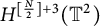 ${H^{ [\frac {N}{2}] +3}}( \mathbb {T} ^2)$
is a Banach algebra, we can bound the rest terms in
 $\left \lVert {f}_2 \right \rVert _{H^{ [\frac {N}{2}] +3}}^2$
as
 $$ \begin{align*} \left\lVert \mathbf{H} \cdot\nabla \mathbf{H} + \mathbf{H} \nabla \mathbf{H} \right\rVert_{H^{ [\frac{N}{2}] +3}}^2 & \le\, C\left\lVert \mathbf{H} \right\rVert_{H^{ [\frac{N}{2}] +3}}^2\left\lVert \nabla \mathbf{H} \right\rVert_{H^{ [\frac{N}{2}] +3}}^2\nonumber\\ & \le\, C\left\lVert \mathbf{H} \right\rVert_{H^{N}}^2\left\lVert \nabla \mathbf{H} \right\rVert_{H^{ [\frac{N}{2}] +4}}^2. \end{align*} $$
 $$ \begin{align*} \left\lVert I(a)( \mathbf{H} \cdot\nabla \mathbf{H} + \mathbf{H} \nabla \mathbf{H} ) \right\rVert_{H^{ [\frac{N}{2}] +3}}^2 & \le\, C\left\lVert I(a) \right\rVert_{H^{ [\frac{N}{2}] +3}}^2\left\lVert \mathbf{H} \right\rVert_{H^{ [\frac{N}{2}] +3}}^2\left\lVert \nabla \mathbf{H} \right\rVert_{H^{ [\frac{N}{2}] +3}}^2\nonumber\\ & \le\, C\left\lVert a \right\rVert_{H^{N}}^2\left\lVert \mathbf{H} \right\rVert_{H^{N}}^2\left\lVert \nabla \mathbf{H} \right\rVert_{H^{ [\frac{N}{2}] +4}}^2. \end{align*} $$
 $$ \begin{align*} \left\lVert k(a)\nabla a \right\rVert_{H^{ [\frac{N}{2}] +3}}^2 \le C\left\lVert k(a) \right\rVert_{H^{ [\frac{N}{2}] +3}}^2\left\lVert \nabla a \right\rVert_{H^{ [\frac{N}{2}] +3}}^2 \le C\left\lVert a \right\rVert_{H^{N}}^2\left\lVert a \right\rVert_{H^{ [\frac{N}{2}] +4}}^2. \end{align*} $$
 $$ \begin{align*} \left\lVert I(a) \nabla \text{ div}\, \mathbf{u} \right\rVert_{H^{ [\frac{N}{2}] +3}}^2 & \le\, C\left\lVert I(a) \right\rVert_{H^{ [\frac{N}{2}] +3}}^2\left\lVert \nabla \text{ div}\, \mathbf{u} \right\rVert_{H^{ [\frac{N}{2}] +3}}^2\nonumber\\ & \le\, C\left\lVert a \right\rVert_{H^{N}}^2\left\lVert \text{div}\, \mathbf{u} \right\rVert_{H^{ [\frac{N}{2}] +4}}^2. \end{align*} $$
 $$ \begin{align*} \left\lVert I(a)( \partial _2 \mathbf{H} -\nabla \mathbf{H} _2) \right\rVert_{H^{ [\frac{N}{2}] +3}}^2 & \le\, C\left\lVert I(a) \right\rVert_{H^{ [\frac{N}{2}] +3}}^2\left\lVert \nabla \mathbf{H} \right\rVert_{H^{ [\frac{N}{2}] +3}}^2\nonumber\\ & \le\, C\left\lVert a \right\rVert_{H^{N}}^2\left\lVert \nabla \mathbf{H} \right\rVert_{H^{ [\frac{N}{2}] +4}}^2. \end{align*} $$
Hence, we get
 $$ \begin{align} \left|{J}_{ 1}^{(6)}\right|& \le\, C\delta^2\left\lVert \partial_2 \mathbf{u} \right\rVert_{H^{ [\frac{N}{2}] +3}}^2\nonumber\\ &+C\delta^2\left\lVert a \right\rVert_{H^{ [\frac{N}{2}] +4}}^2+ C\left\lVert \nabla \mathbf{H} \right\rVert_{H^{ [\frac{N}{2}] +4}}^2+C\left\lVert \text{div}\, \mathbf{u} \right\rVert_{H^{ [\frac{N}{2}] +4}}^2. \end{align} $$
Applying the Hölder inequality and the Young inequality, we have
 $$ \begin{align} J_2 \le&\frac{1}{16}\left\lVert {\Lambda^s}\partial_2 \mathbf{u} \right\rVert_{L^2}^2+C\left\lVert \nabla \mathbf{H} \right\rVert_{H^{ [\frac{N}{2}] +4}}^2, \end{align} $$
 $$ \begin{align} {J}_{ 3} \le&\frac{1}{16}\left\lVert {\Lambda^s}\partial_2 \mathbf{u} \right\rVert_{L^2}^2+C\left\lVert \text{div}\, \mathbf{u} \right\rVert_{H^{ [\frac{N}{2}] +4}}^2. \end{align} $$
We now turn to the last term
 ${J}_{ 4}$
. We first rewrite it into
 $$ \begin{align*} {J}_{ 4} &=-{\int_{\mathbb{T} ^2}{\Lambda^s} ( \mathbf{u} \cdot\nabla \mathbf{H} ){\cdot}{\Lambda^s}\partial_2 \mathbf{u} \,dx} +{\int_{\mathbb{T} ^2}{\Lambda^s} ( \mathbf{H} \cdot\nabla \mathbf{u} - \mathbf{H} \text{ div}\, \mathbf{u} ){\cdot}{\Lambda^s}\partial_2 \mathbf{u} \,dx} \nonumber\\&={J}_{ 4,1}+{J}_{ 4,2}. \end{align*} $$
Thanks to the Hölder inequality and the Young inequality,
 $$ \begin{align*} {J}_{ 4,1} \le&\, C\left\lVert {\Lambda^s}( \mathbf{u} \cdot\nabla \mathbf{H} ) \right\rVert_{L^2}\left\lVert {\Lambda^s}\partial_2 \mathbf{u} \right\rVert_{L^2}\nonumber\\ \le&\, C(\left\lVert \mathbf{u} \right\rVert_{L^\infty}\left\lVert \nabla \mathbf{H} \right\rVert_{H^s}+\left\lVert \nabla \mathbf{H} \right\rVert_{L^\infty}\left\lVert \mathbf{u} \right\rVert_{H^s} )\left\lVert {\Lambda^s}\partial_2 \mathbf{u} \right\rVert_{L^2}\nonumber\\ \le&\,\frac{1}{16}\left\lVert {\Lambda^s}\partial_2 \mathbf{u} \right\rVert_{L^2}^2+C\left\lVert \mathbf{u} \right\rVert_{H^N}^2\left\lVert \nabla \mathbf{H} \right\rVert_{H^{ [\frac{N}{2}] +4}}^2\nonumber\\ \le&\,\frac{1}{16}\left\lVert {\Lambda^s}\partial_2 \mathbf{u} \right\rVert_{L^2}^2+C\delta^2\left\lVert \nabla \mathbf{H} \right\rVert_{H^{ [\frac{N}{2}] +4}}^2, \end{align*} $$
and
 $$ \begin{align*} {J}_{ 4,2} \le&\, C\left\lVert {\Lambda^s}( \mathbf{H} \cdot\nabla \mathbf{u} - \mathbf{H} \text{ div}\, \mathbf{u} ) \right\rVert_{L^2}\left\lVert {\Lambda^s}\partial_2 \mathbf{u} \right\rVert_{L^2}\nonumber\\ \le&\, C(\left\lVert \mathbf{H} \right\rVert_{L^\infty}\left\lVert \nabla \mathbf{u} \right\rVert_{H^s}+\left\lVert \nabla \mathbf{u} \right\rVert_{L^\infty}\left\lVert \mathbf{H} \right\rVert_{H^s} )\left\lVert {\Lambda^s}\partial_2 \mathbf{u} \right\rVert_{L^2}\nonumber\\ \le&\,\frac{1}{16}\left\lVert {\Lambda^s}\partial_2 \mathbf{u} \right\rVert_{L^2}^2+C\left\lVert \mathbf{u} \right\rVert_{H^N}^2(\left\lVert \mathbf{H} \right\rVert_{H^{s}}^2+\left\lVert \mathbf{H} \right\rVert_{H^{2}}^2)\nonumber\\ \le&\,\frac{1}{16}\left\lVert {\Lambda^s}\partial_2 \mathbf{u} \right\rVert_{L^2}^2+C\delta^2\left\lVert \nabla \mathbf{H} \right\rVert_{H^{ [\frac{N}{2}] +4}}^2. \end{align*} $$
Hence,
 $$ \begin{align} {J}_{ 4} \le&\frac{1}{8}\left\lVert {\Lambda^s}\partial_2 \mathbf{u} \right\rVert_{L^2}^2+C\delta^2\left\lVert \nabla \mathbf{H} \right\rVert_{H^{ [\frac{N}{2}] +4}}^2. \end{align} $$
Inserting (3.41)–(3.43) in (3.40) and then combining with (3.44)–(3.46), we get from (3.39) that
 $$ \begin{align} &\frac12\left\lVert {\Lambda^s}\partial_2 \mathbf{u} \right\rVert_{L^2}^2-\frac{d}{dt}\int_{\mathbb{T} ^2}{\Lambda^s} \mathbf{H} \cdot{\Lambda^s}\partial_2 \mathbf{u} \,dx\nonumber\\ &\quad\le C\delta^2\left\lVert a \right\rVert_{H^{ [\frac{N}{2}] +4}}^2+ C\left\lVert \nabla \mathbf{H} \right\rVert_{H^{ [\frac{N}{2}] +4}}^2+C\left\lVert \text{div}\, \mathbf{u} \right\rVert_{H^{ [\frac{N}{2}] +4}}^2. \end{align} $$
Summing (3.47) over
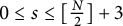 $0\le s\le [\frac {N}{2}] +3$
, we arrive at (3.38), hence, we complete the proof of Lemma 3.4.
3.4 The dissipation of the density
The aim of this section is to prove the following key lemma.
Lemma 3.5 Let
 ${N}\ge 12$
. Let
 $(a, \mathbf {u} , \mathbf {H} ) \in C([0, T];H^N)$
be a solution to the system (3.2). Assume that
 $$ \begin{align*} \sup_{t\in[0,T]}(\left\lVert a \right\rVert_{H^{N}}+\left\lVert \mathbf{u} \right\rVert_{H^{N}}+\left\lVert \mathbf{H} \right\rVert_{H^{N}})\le \delta, \end{align*} $$
for some
 $0<\delta <1.$
Then there holds that
 $$ \begin{align} &\frac{d}{dt}\left\lVert (a, \mathbf{G} ) \right\rVert_{H^{ [\frac{N}{2}] +4}}^2+\frac{1}{\nu}\left\lVert {a} \right\rVert_{H^{ [\frac{N}{2}] +4}}^2+\nu\left\lVert \nabla \mathbf{G} \right\rVert_{H^{ [\frac{N}{2}] +4}}^2\nonumber\\&\quad\le C\delta^2\left\lVert \partial_2 \mathbf{u} \right\rVert_{H^{ [\frac{N}{2}] +3}}^2+C\delta^2\left\lVert a \right\rVert_{H^{ [\frac{N}{2}] +4}}^2\nonumber\\&\qquad+ C\left\lVert \nabla \mathbf{H} \right\rVert_{H^{ [\frac{N}{2}] +4}}^2+C\left\lVert \mathrm{div}\, \mathbf{u} \right\rVert_{H^{ [\frac{N}{2}] +4}}^2. \end{align} $$
Proof First of all, applying the operator
 ${\mathbb {Q}}$
to the velocity equation in (3.2) yields
 $$ \begin{align*} &\partial_t {\mathbb{Q}} \mathbf{u} -\nu\Delta {\mathbb{Q}} \mathbf{u} +\nabla a+\nabla \mathbf{H} _2={\mathbb{Q}} f_4. \end{align*} $$
To find the dissipation of a, here we perform the energy argument in terms of the effective velocity
 $$ \begin{align} \mathbf{G} \stackrel{\mathrm{def}}{=}{\mathbb{Q}} \mathbf{u} -\frac1\nu\Delta^{-1}\nabla {a}. \end{align} $$
Note that if (3.49) is written in terms of
 $a,\, \mathbf {G} $
and of the divergence free part
 ${\mathbb {Q}} \mathbf {u} $
of
 $ \mathbf {u} ,$
then, up to low-order terms, a satisfies a damped transport equation, and
 $ \mathbf {G} $
satisfies a heat equation. By the definition of
 $\mathbb {Q} = \nabla \Delta ^{-1} \text { div}\, $
, we note that
 $$ \begin{align*}\text{div}\, \mathbf{u} = \text{div}\, \mathbb{Q} \mathbf{u} = \text{div}\, \mathbf{G} + \frac1\nu a. \end{align*} $$
On the one hand, it is clear that
 $ \mathbf {G} $
fulfills
 $$ \begin{align} \partial_t \mathbf{G} -\nu\Delta \mathbf{G} =\frac1\nu{\mathbb{Q}} \mathbf{u} -\nabla \mathbf{H} _2 +{\mathbb{Q}} f_4-\frac1\nu\Delta^{-1}\nabla f_1. \end{align} $$
On the one hand, in terms of
 $ \mathbf {G} ,$
the function a satisfies the following damped transport equation:
 $$ \begin{align*}\partial_t a +\frac1\nu{a}+ \text{ div}\, \mathbf{G} =f_1.\end{align*} $$
Hence, arguing exactly as for proving (3.11) shows that
 $$ \begin{align} &\frac12\frac{d}{dt}\left\lVert \Lambda ^m {a} \right\rVert_{L^{2}}^2+\frac1\nu\left\lVert \Lambda ^m {a} \right\rVert_{L^{2}}^2\nonumber\\&\quad=-\int_{\mathbb{T} ^2} \Lambda ^m \text{ div}\, \mathbf{G} \cdot \Lambda ^m {a}\,dx+\int_{\mathbb{T} ^2} \Lambda ^m f_1\cdot \Lambda ^m {a}\,dx. \end{align} $$
Thanks to the Hölder inequality and the Young inequality, there holds
 $$ \begin{align*} \left|-\int_{\mathbb{T} ^2} \Lambda ^m \text{ div}\, \mathbf{G} \cdot \Lambda ^m {a}\,dx\right| &\le\| \Lambda ^m \text{ div}\, \mathbf{G} \|_{L^2}\| \Lambda ^ma\|_{L^2}\nonumber\\&\le\frac{1}{2\nu}\| \Lambda ^ma\|_{L^2}^2+C\| \Lambda ^{m+1} \mathbf{G} \|_{L^2}^2. \end{align*} $$
The last term in (3.51) can be bounded the same as (3.21)
 $$ \begin{align*} \left|\int_{\mathbb{T} ^2} \Lambda ^{m} f_1\cdot \Lambda ^{m} a\,dx\right| &\le\frac{c_0^{-1}\nu}{16}\| \text{div}\, \mathbf{u} \|_{H^{m}}^2\nonumber\\&\quad +C\left\lVert (\nabla a,\nabla \mathbf{u} ) \right\rVert_{L^\infty}+\|a\|_{L^{\infty}}^2)\left\lVert ( \Lambda ^{m}a, \Lambda ^{m} \mathbf{u} ) \right\rVert_{L^2}^2 \end{align*} $$
from which we have
 $$ \begin{align} &\frac12\frac{d}{dt}\left\lVert {a} \right\rVert_{H^{m}}^2+\frac{1}{2\nu}\left\lVert {a} \right\rVert_{H^{m}}^2\nonumber\\ &\quad\le \frac{c_0^{-1}\nu}{16}\| \text{div}\, \mathbf{u} \|_{H^{m}}^2+C\delta^2\left\lVert a \right\rVert_{H^{ [\frac{N}{2}] +4}}^2\nonumber\\ &\qquad+C\left\lVert \nabla \mathbf{G} \right\rVert_{H^{m}}^{2}+C(\left\lVert (\nabla a,\nabla \mathbf{u} ) \right\rVert_{L^\infty}+\|a\|_{L^{\infty}}^2)\left\lVert (a, \mathbf{u} ) \right\rVert_{H^m}^2. \end{align} $$
Similarly, for any
 $m\ge 0$
, applying
 ${ \Lambda ^m}$
to (3.50) and multiplying it by
 ${ \Lambda ^m}{ \mathbf {G} }$
lead to
 $$ \begin{align*} &\frac12\frac{d}{dt}\left\lVert \Lambda ^{m} \mathbf{G} \right\rVert_{L^{2}}^2+\nu\left\lVert \Lambda ^{m} \nabla \mathbf{G} \right\rVert_{L^{2}}^2\nonumber\\ &\quad=\frac1\nu\int_{\mathbb{T} ^2} \Lambda ^m{\mathbb{Q}} \mathbf{u} \cdot \Lambda ^m \mathbf{G} \,dx -\int_{\mathbb{T} ^2} \Lambda ^m\nabla \mathbf{H} _2\cdot \Lambda ^m \mathbf{G} \,dx\nonumber\\ &\qquad +\int_{\mathbb{T} ^2} \Lambda ^m{\mathbb{Q}} f_4\cdot \Lambda ^m \mathbf{G} \,dx+\frac1\nu\int_{\mathbb{T} ^2} \Lambda ^m\Delta^{-1}\nabla f_1\cdot \Lambda ^m \mathbf{G} \,dx. \end{align*} $$
For
 $m=0,$
we get by the Young inequality and the Poincaré inequality that
 $$ \begin{align} &\frac12\frac{d}{dt}\left\lVert \mathbf{G} \right\rVert_{L^{2}}^2+\nu\left\lVert \nabla \mathbf{G} \right\rVert_{L^{2}}^2\nonumber\\&\quad=\frac1\nu\int_{\mathbb{T} ^2}{\mathbb{Q}} \mathbf{u} \cdot \mathbf{G} \,dx -\int_{\mathbb{T} ^2}\nabla \mathbf{H} _2\cdot \mathbf{G} \,dx \nonumber\\&\qquad+\int_{\mathbb{T} ^2}{\mathbb{Q}} f_4\cdot \mathbf{G} \,dx+\frac1\nu\int_{\mathbb{T} ^2}\Delta^{-1}\nabla f_1\cdot \mathbf{G} \,dx\nonumber\\&\quad\le C(\left\lVert \text{div}\, \mathbf{u} \right\rVert_{H^{-1}}+\left\lVert \mathbf{H} \right\rVert_{L^{2}}+\left\lVert f_4 \right\rVert_{L^{2}} +\left\lVert \Delta^{-1}\nabla f_1 \right\rVert_{L^{2}})\left\lVert \mathbf{G} \right\rVert_{L^{2}}\nonumber\\&\quad\le \frac{\nu}{2}\left\lVert \nabla \mathbf{G} \right\rVert_{L^{2}}^2+ C(\left\lVert \text{div}\, \mathbf{u} \right\rVert_{H^{-1}}^2+\left\lVert f_1 \right\rVert_{H^{-1}}^2 +\left\lVert f_4 \right\rVert_{L^2}^2). \end{align} $$
For
 $1\le m\le N,$
we get by the integration by parts and the Young inequality that
 $$ \begin{align*} &\frac12\frac{d}{dt}\left\lVert \Lambda ^{m} \mathbf{G} \right\rVert_{L^{2}}^2+\nu\left\lVert \Lambda ^{m} \nabla \mathbf{G} \right\rVert_{L^{2}}^2\nonumber\\ &\quad=\frac1\nu\int_{\mathbb{T} ^2} \Lambda ^m{\mathbb{Q}} \mathbf{u} \cdot \Lambda ^m \mathbf{G} \,dx-\int_{\mathbb{T} ^2} \Lambda ^m\nabla \mathbf{H} _2\cdot \Lambda ^m \mathbf{G} \,dx\nonumber\\ &\qquad+\int_{\mathbb{T} ^2} \Lambda ^m{\mathbb{Q}} f_4\cdot \Lambda ^m \mathbf{G} \,dx+\frac1\nu\int_{\mathbb{T} ^2} \Lambda ^m\Delta^{-1}\nabla f_1\cdot \Lambda ^m \mathbf{G} \,dx\nonumber\\ &\quad\le C(\left\lVert \Lambda ^{m-1}{\mathbb{Q}} \mathbf{u} \right\rVert_{L^{2}}+\left\lVert \Lambda ^{m-1}f_4 \right\rVert_{L^{2}}+\left\lVert \Lambda ^{m} \mathbf{H} \right\rVert_{L^{2}} +\left\lVert \Lambda ^{m-2}f_1 \right\rVert_{L^{2}})\left\lVert \Lambda ^{m +1} \mathbf{G} \right\rVert_{L^{2}}\nonumber\\ &\quad\le\frac\nu4\left\lVert \Lambda ^{m+1} \mathbf{G} \right\rVert_{L^{2}}^2 +C\left\lVert \Lambda ^{m-1}{\mathbb{Q}} \mathbf{u} \right\rVert_{L^{2}}^2+C\left\lVert \Lambda ^{m} \mathbf{H} \right\rVert_{L^{2}}^2\nonumber\\ &\qquad+C\left\lVert \Lambda ^{m-2}f_1 \right\rVert_{L^{2}}^2 +C\left\lVert \Lambda ^{m-1}f_4 \right\rVert_{L^{2}}^2\nonumber\\ &\quad\le\frac\nu4\left\lVert \Lambda ^{m+1} \mathbf{G} \right\rVert_{L^{2}}^2 +C\left\lVert \Lambda ^{m-3} \text{ div}\, \mathbf{u} \right\rVert_{L^{2}}^2 +C\left\lVert \Lambda ^{m} \mathbf{H} \right\rVert_{L^{2}}^2\nonumber\\ &\qquad+C\left\lVert \Lambda ^{m-2}f_1 \right\rVert_{L^{2}}^2+C\left\lVert \Lambda ^{m-1}f_4 \right\rVert_{L^{2}}^2 \end{align*} $$
from which we have
 $$ \begin{align} &\frac12\frac{d}{dt}\left\lVert \Lambda ^{m} \mathbf{G} \right\rVert_{L^{2}}^2+\frac\nu2\left\lVert \Lambda ^{m} \nabla \mathbf{G} \right\rVert_{L^{2}}^2\nonumber\\ &\quad\le C\big(\left\lVert \Lambda ^{m-3} \text{ div}\, \mathbf{u} \right\rVert_{L^{2}}^2+\left\lVert \Lambda ^{m} \mathbf{H} \right\rVert_{L^{2}}^2+\left\lVert \Lambda ^{m-2}f_1 \right\rVert_{L^{2}}^2 +\left\lVert \Lambda ^{m-1}f_4 \right\rVert_{L^{2}}^2\big). \end{align} $$
Combining with (3.53) and (3.54), we get, for any
 $m\ge 0$
, that
 $$ \begin{align} &\frac12\frac{d}{dt}\left\lVert \mathbf{G} \right\rVert_{H^{m}}^2+\frac\nu2\left\lVert \nabla \mathbf{G} \right\rVert_{H^{m}}^2\nonumber\\ &\quad\le C\big(\left\lVert \text{div}\, \mathbf{u} \right\rVert_{H^{m}}^2+\left\lVert \mathbf{H} \right\rVert_{H^{m}}^2+\left\lVert f_1 \right\rVert_{H^{-1}}^2 +\left\lVert f_1 \right\rVert_{H^{m-2}}^2+\left\lVert f_4 \right\rVert_{L^2}^2 +\left\lVert f_4 \right\rVert_{H^{m-1}}^2\big). \end{align} $$
Multiplying (3.55) by a suitable large constant and then adding to (3.52), we get
 $$ \begin{align} &\frac{d}{dt}\left\lVert (a, \mathbf{G} ) \right\rVert_{H^{m}}^2+\frac{1}{\nu}\left\lVert {a} \right\rVert_{H^{m}}^2+\nu\left\lVert \nabla \mathbf{G} \right\rVert_{H^{m}}^2\nonumber\\ &\quad\le C\big(\left\lVert \text{div}\, \mathbf{u} \right\rVert_{H^{m}}^2+\left\lVert \mathbf{H} \right\rVert_{H^{m}}^2+\left\lVert f_1 \right\rVert_{H^{-1}}^2 +\left\lVert f_1 \right\rVert_{H^{m-2}}^2+\left\lVert f_4 \right\rVert_{L^2}^2 +\left\lVert f_4 \right\rVert_{H^{m-1}}^2\big). \end{align} $$
Especially, taking
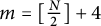 $m= [\frac {N}{2}] +4$
in (3.56) gives
 $$ \begin{align} &\frac{d}{dt}\left\lVert (a, \mathbf{G} ) \right\rVert_{H^{ [\frac{N}{2}] +4}}^2+\frac{1}{\nu}\left\lVert {a} \right\rVert_{H^{ [\frac{N}{2}] +4}}^2+\nu\left\lVert \nabla \mathbf{G} \right\rVert_{H^{ [\frac{N}{2}] +4}}^2\nonumber\\ &\quad\le C\big(\left\lVert \text{div}\, \mathbf{u} \right\rVert_{H^{ [\frac{N}{2}] +4}}^2+\left\lVert \mathbf{H} \right\rVert_{H^{ [\frac{N}{2}] +4}}^2 +\left\lVert f_1 \right\rVert_{H^{ [\frac{N}{2}] +2}}^2 +\left\lVert f_4 \right\rVert_{H^{ [\frac{N}{2}] +3}}^2\big). \end{align} $$
By Lemma 2.5,
 $$ \begin{align} \left\lVert f_1 \right\rVert_{H^{ [\frac{N}{2}] +2}}^2 &\le C\left\lVert a \mathbf{u} \right\rVert_{H^{ [\frac{N}{2}] +3}}^2\nonumber\\&\le C\left\lVert a \right\rVert_{H^{ [\frac{N}{2}] +3}}^2\left\lVert \mathbf{u} \right\rVert_{H^{ [\frac{N}{2}] +3}}^2\nonumber\\&\le C\left\lVert \mathbf{u} \right\rVert_{H^{N}}^2\left\lVert a \right\rVert_{H^{ [\frac{N}{2}] +4}}^2\nonumber\\&\le C\delta^2\left\lVert a \right\rVert_{H^{{ [\frac{N}{2}] +4}}}^2. \end{align} $$
The estimation of
 $\left \lVert f_4 \right \rVert _{H^{ [\frac {N}{2}] +3}}^2$
can be obtained from (3.43). Hence, inserting (3.58) and (3.43) into (3.57) implies that (3.48). We complete the proof of this lemma.
3.5 Lyapunov-type differential inequality
In this section, we establish the Lyapunov-type inequality in time for low-order energy norms, which leads to the time-decay estimates. More precisely, we shall prove the following lemma.
Lemma 3.6 Let
 ${N}\ge 12$
. Let
 $(a, \mathbf {u} , \mathbf {H} ) \in C([0, T];H^N)$
be a solution to the system (3.2). Assume that
 $$ \begin{align*} \sup_{t\in[0,T]}(\left\lVert a \right\rVert_{H^{N}}+\left\lVert \mathbf{u} \right\rVert_{H^{N}}+\left\lVert \mathbf{H} \right\rVert_{H^{N}})\le \delta, \end{align*} $$
for some
 $0<\delta <1.$
Then, for some large constant
 $\eta $
, the quantity
 $$ \begin{align*} {\mathcal{E}(t)}=&\eta\left\lVert (a, \mathbf{u} , \mathbf{H} , \mathbf{G} ) \right\rVert_{H^{{ [\frac{N}{2}] +4}}}^2-\sum_{0\le s\le { [\frac{N}{2}] +3}}\int_{\mathbb{T} ^2} \Lambda ^{s} \mathbf{H} \cdot \Lambda ^{s}\partial_2 \mathbf{u} \,dx \end{align*} $$
satisfies
 $$ \begin{align*} \frac{d}{dt}{\mathcal{E}(t)}+c({\mathcal{E}(t)})^{\frac43}\le 0. \end{align*} $$
Proof Taking
 $\ell = [\frac {N}{2}] +4$
in (3.10) gives
 $$ \begin{align} &\frac12\frac{d}{dt}\left\lVert (a, \mathbf{u} , \mathbf{H} ) \right\rVert_{H^{ [\frac{N}{2}] +4}}^2 +\nu\left\lVert \text{div}\, \mathbf{u} \right\rVert_{H^{ [\frac{N}{2}] +4}}^2+\sigma\left\lVert \nabla \mathbf{H} \right\rVert_{H^{ [\frac{N}{2}] +4}}^2 \nonumber\\&\quad\le C \mathrm{Y}^{( [\frac{N}{2}] +4)}_{\infty}(t)\left\lVert (a, \mathbf{u} , \mathbf{H} ) \right\rVert_{H^{ [\frac{N}{2}] +4}}^2. \end{align} $$
Multiplying (3.59) by a suitable large constant and then adding to (3.48) lead to
 $$ \begin{align} &\frac{d}{dt}\left\lVert (a, \mathbf{u} , \mathbf{H} , \mathbf{G} ) \right\rVert_{H^{{ [\frac{N}{2}] +4}}}^2+\frac{1}{\nu}\left\lVert {a} \right\rVert_{H^{ [\frac{N}{2}] +4}}^2\nonumber\\ &\qquad+\nu\left\lVert \text{div}\, \mathbf{u} \right\rVert_{H^{{ [\frac{N}{2}] +4}}}^2 +\nu\left\lVert \nabla \mathbf{G} \right\rVert_{H^{ [\frac{N}{2}] +4}}^2+\sigma\left\lVert \nabla \mathbf{H} \right\rVert_{H^{ [\frac{N}{2}] +4}}^2\\ &\quad\le C\delta^2\left\lVert \partial_2 \mathbf{u} \right\rVert_{H^{ [\frac{N}{2}] +3}}^2+C\delta^2\left\lVert a \right\rVert_{H^{ [\frac{N}{2}] +4}}^2 + C \mathrm{Y}^{( [\frac{N}{2}] +4)}_{\infty}(t)\left\lVert (a, \mathbf{u} , \mathbf{H} ) \right\rVert_{H^{ [\frac{N}{2}] +4}}^2.\nonumber \end{align} $$
Multiplying (3.60) by a suitable large constant
 $\eta $
and adding to (3.38) give rise to
 $$ \begin{align} &\frac{d}{dt}\Bigg\{\eta\Big(\left\lVert (a, \mathbf{u} , \mathbf{H} , \mathbf{G} ) \right\rVert_{H^{{ [\frac{N}{2}] +4}}}^2\Big)-\sum_{0\le s\le {r+3}}\int_{\mathbb{T} ^2} \Lambda ^{s} \mathbf{H} \cdot \Lambda ^{s}\partial_2 \mathbf{u} \,dx\Bigg\} \nonumber\\ &\qquad +\left\lVert \partial_2 \mathbf{u} \right\rVert_{H^{ [\frac{N}{2}] +3}}^2+\eta\Big(\frac{1}{\nu}\left\lVert {a} \right\rVert_{H^{ [\frac{N}{2}] +4}}^2+\nu\left\lVert \text{div}\, \mathbf{u} \right\rVert_{H^{{ [\frac{N}{2}] +4}}}^2 \nonumber\\ &\qquad\qquad\qquad\qquad\qquad\qquad+\sigma\left\lVert \nabla \mathbf{H} \right\rVert_{H^{{ [\frac{N}{2}] +4}}}^2+\nu\left\lVert \nabla \mathbf{G} \right\rVert_{H^{ [\frac{N}{2}] +4}}^2\Big)\nonumber\\ &\quad\le C\delta^2\left\lVert \partial_2 \mathbf{u} \right\rVert_{H^{ [\frac{N}{2}] +3}}^2+C\delta^2\left\lVert a \right\rVert_{H^{ [\frac{N}{2}] +4}}^2 \nonumber\\ &\qquad+ C \mathrm{Y}^{( [\frac{N}{2}] +4)}_{\infty}(t)\left\lVert (a, \mathbf{u} , \mathbf{H} ) \right\rVert_{H^{ [\frac{N}{2}] +4}}^2. \end{align} $$
It’s not hard to check, for any
 $\ell>7,$
that
 $$ \begin{align} \left\lVert a \right\rVert_{H^{[\frac{\ell-1}{2}]+4}} & \le\, C\left\lVert a \right\rVert_{H^{\ell}};\nonumber\\ \left\lVert \text{div}\, \mathbf{u} \right\rVert_{H^{\ell-[\frac{\ell-1}{2}]}}& \le\, C\left\lVert \text{div}\, \mathbf{u} \right\rVert_{H^{\ell}}. \end{align} $$
With the aid of the Sobolev embedding relation, we have
 $$ \begin{align*} \mathrm{Y}_{\infty}^{( [\frac{N}{2}] +4)}(t) & \le\, C\big(\left\lVert ( \mathbf{u} , \mathbf{H} ) \right\rVert_{H^{3}} +\left\lVert a \right\rVert_{H^{ [\frac{N}{2}] +4}}+\left\lVert \text{div}\, \mathbf{u} \right\rVert_{H^{ [\frac{N}{2}] +4}} \nonumber\\ &\quad+\left\lVert (a, \mathbf{u} , \mathbf{H} ) \right\rVert_{H^{3}}^2 +\left\lVert a \right\rVert_{H^{3}}^2\left\lVert \mathbf{H} \right\rVert_{H^{3}}^2+\left\lVert \mathbf{H} \right\rVert_{H^{3}}^4 +\left\lVert a \right\rVert_{H^{ [\frac{N}{2}] +4}}^2\big). \end{align*} $$
Hence, for any
 $N\ge 7,$
there holds
 $$ \begin{align} &\mathrm{Y}_{\infty}^{( [\frac{N}{2}] +4)}(t)\left\lVert (a, \mathbf{H} ) \right\rVert_{H^{ [\frac{N}{2}] +4}}^2\nonumber\\ &\quad\le C\left\lVert (a, \mathbf{u} , \mathbf{H} ) \right\rVert_{H^{N}}\left\lVert (a, \mathbf{H} ) \right\rVert_{H^{ [\frac{N}{2}] +4}}^2\nonumber\\ &\qquad+C(\left\lVert (a, \mathbf{u} , \mathbf{H} ) \right\rVert_{H^{N}}^2 +\left\lVert a \right\rVert_{H^{N}}^2\left\lVert \mathbf{H} \right\rVert_{H^{N}}^2+\left\lVert \mathbf{H} \right\rVert_{H^{N}}^4)\left\lVert (a, \mathbf{H} ) \right\rVert_{H^{ [\frac{N}{2}] +4}}^2\nonumber\\ &\quad\le C\delta(1+\delta^3)\left\lVert (a, \mathbf{H} ) \right\rVert_{H^{ [\frac{N}{2}] +4}}^2. \end{align} $$
Due to lack of dissipation for the incompressible part of
 $ \mathbf {u} $
, the estimate about
 $$ \begin{align*}\mathrm{Y}_{\infty}^{( [\frac{N}{2}] +4)}(t)\left\lVert \mathbf{u} \right\rVert_{H^{ [\frac{N}{2}] +4}}^2\end{align*} $$
is more refined. By using the fact that (3.62), we have
 $$ \begin{align} &\mathrm{Y}_{\infty}^{( [\frac{N}{2}] +4)}(t)\left\lVert \mathbf{u} \right\rVert_{H^{ [\frac{N}{2}] +4}}^2\nonumber\\ &\quad\le C(\left\lVert ( \mathbf{u} , \mathbf{H} ) \right\rVert_{H^{3}} +\left\lVert a \right\rVert_{H^{ [\frac{N}{2}] +4}}+\left\lVert \text{div}\, \mathbf{u} \right\rVert_{H^{ [\frac{N}{2}] +4}} \\ &\qquad+\left\lVert (a, \mathbf{u} , \mathbf{H} ) \right\rVert_{H^{3}}^2 +\left\lVert a \right\rVert_{H^{3}}^2\left\lVert \mathbf{H} \right\rVert_{H^{3}}^2+\left\lVert \mathbf{H} \right\rVert_{H^{3}}^4 +\left\lVert a \right\rVert_{H^{ [\frac{N}{2}] +4}}^2)\left\lVert \mathbf{u} \right\rVert_{H^{ [\frac{N}{2}] +4}}^2.\nonumber \end{align} $$
By Proposition 2.3, there holds
 $$ \begin{align*} \left\lVert \mathbf{u} \right\rVert_{H^{3}}\le C\left\lVert \nabla \mathbf{u} \right\rVert_{H^{2}}\le C\left\lVert \partial_2 \mathbf{u} \right\rVert_{H^{3}}+\left\lVert \text{div}\, \mathbf{u} \right\rVert_{H^{2}} \end{align*} $$
from which we have
 $$ \begin{align} &(\left\lVert ( \mathbf{u} , \mathbf{H} ) \right\rVert_{H^{3}} +\left\lVert a \right\rVert_{H^{ [\frac{N}{2}] +4}}+\left\lVert \text{div}\, \mathbf{u} \right\rVert_{H^{ [\frac{N}{2}] +4}})\left\lVert \mathbf{u} \right\rVert_{H^{ [\frac{N}{2}] +4}}^2\nonumber\\&\quad\le C(\left\lVert (a, \mathbf{H} ) \right\rVert_{H^{ [\frac{N}{2}] +4}}+\left\lVert \partial_2 \mathbf{u} \right\rVert_{H^{ [\frac{N}{2}] +3}}+\left\lVert \text{div}\, \mathbf{u} \right\rVert_{H^{ [\frac{N}{2}] +4}})\left\lVert \mathbf{u} \right\rVert_{H^{ [\frac{N}{2}] +4}}^2\nonumber\\&\quad\le \delta^2\left(\left\lVert (a, \mathbf{H} ) \right\rVert_{H^{ [\frac{N}{2}] +4}}^2+\left\lVert \partial_2 \mathbf{u} \right\rVert_{H^{ [\frac{N}{2}] +3}}^2 +\left\lVert \text{div}\, \mathbf{u} \right\rVert_{H^{ [\frac{N}{2}] +4}}^2\right)+C\left\lVert \mathbf{u} \right\rVert_{H^{ [\frac{N}{2}] +4}}^4, \end{align} $$
 $$ \begin{align} &(\left\lVert (a, \mathbf{u} , \mathbf{H} ) \right\rVert_{H^{3}}^2 +\left\lVert a \right\rVert_{H^{ [\frac{N}{2}] +4}}^2)\left\lVert \mathbf{u} \right\rVert_{H^{ [\frac{N}{2}] +4}}^2 \nonumber\\ &\quad\le C(\left\lVert (a, \mathbf{H} ) \right\rVert_{H^{ [\frac{N}{2}] +4}}^2+\left\lVert \partial_2 \mathbf{u} \right\rVert_{H^{3}}^2+\left\lVert \text{div}\, \mathbf{u} \right\rVert_{H^{2}}^2)\left\lVert \mathbf{u} \right\rVert_{H^{ [\frac{N}{2}] +4}}^2\nonumber\\ &\quad\le C\left\lVert \mathbf{u} \right\rVert_{H^{N}}^2(\left\lVert (a, \mathbf{H} ) \right\rVert_{H^{ [\frac{N}{2}] +4}}^2+\left\lVert \partial_2 \mathbf{u} \right\rVert_{H^{ [\frac{N}{2}] +3}}^2+\left\lVert \text{div}\, \mathbf{u} \right\rVert_{H^{ [\frac{N}{2}] +4}}^2)\nonumber\\ &\quad\le C\delta^2(\left\lVert (a, \mathbf{H} ) \right\rVert_{H^{ [\frac{N}{2}] +4}}^2+\left\lVert \partial_2 \mathbf{u} \right\rVert_{H^{ [\frac{N}{2}] +3}}^2+\left\lVert \text{div}\, \mathbf{u} \right\rVert_{H^{ [\frac{N}{2}] +4}}^2) \end{align} $$
and
 $$ \begin{align} &(\left\lVert a \right\rVert_{H^{3}}^2\left\lVert \mathbf{H} \right\rVert_{H^{3}}^2+\left\lVert \mathbf{H} \right\rVert_{H^{3}}^4)\left\lVert \mathbf{u} \right\rVert_{H^{ [\frac{N}{2}] +4}}^2\nonumber\\ &\quad\le C\left\lVert a \right\rVert_{H^{ [\frac{N}{2}] +4}}^2\left\lVert \mathbf{H} \right\rVert_{H^{ [\frac{N}{2}] +4}}^2\left\lVert \mathbf{u} \right\rVert_{H^{ [\frac{N}{2}] +4}}^2+C\left\lVert \mathbf{H} \right\rVert_{H^{ [\frac{N}{2}] +4}}^4\left\lVert \mathbf{u} \right\rVert_{H^{ [\frac{N}{2}] +4}}^2\nonumber\\ &\quad\le C\left\lVert \mathbf{u} \right\rVert_{H^{ [\frac{N}{2}] +4}}^2\left\lVert \mathbf{H} \right\rVert_{H^{ [\frac{N}{2}] +4}}^2(\left\lVert a \right\rVert_{H^{ [\frac{N}{2}] +4}}^2+\left\lVert \mathbf{H} \right\rVert_{H^{ [\frac{N}{2}] +4}}^2)\nonumber\\ &\quad\le C\delta^4\left\lVert (a, \mathbf{H} ) \right\rVert_{H^{ [\frac{N}{2}] +4}}^2. \end{align} $$
Inserting (3.65)–(3.67) into (3.64), we have
 $$ \begin{align*} &\mathrm{Y}_{\infty}^{( [\frac{N}{2}] +4)}(t)\left\lVert \mathbf{u} \right\rVert_{H^{ [\frac{N}{2}] +4}}^2\le C\left\lVert \mathbf{u} \right\rVert_{H^{ [\frac{N}{2}] +4}}^4\nonumber\\ &\quad+C\delta^2(1+\delta^2)(\left\lVert (a, \mathbf{H} ) \right\rVert_{H^{ [\frac{N}{2}] +4}}^2+\left\lVert \text{div}\, \mathbf{u} \right\rVert_{H^{ [\frac{N}{2}] +4}} +\left\lVert \partial_2 \mathbf{u} \right\rVert_{H^{ [\frac{N}{2}] +3}}^2). \end{align*} $$
For any
 ${N}\ge 12$
, from Proposition 2.3, we have
 $$ \begin{align*} \left\lVert \mathbf{u} \right\rVert_{H^{ [\frac{N}{2}] +4}}^2 & \le\, C\left\lVert \nabla \mathbf{u} \right\rVert_{H^{ [\frac{N}{2}] +3}}^4\nonumber\\ & \le\, C\left\lVert \nabla \mathbf{u} \right\rVert_{H^{ [\frac{N}{2}] +2}}\left\lVert \mathbf{u} \right\rVert_{H^{{N}}}\nonumber\\ & \le\, C\delta(\left\lVert \partial_2 \mathbf{u} \right\rVert_{H^{ [\frac{N}{2}] +3}}+\left\lVert \text{div}\, \mathbf{u} \right\rVert_{H^{ [\frac{N}{2}] +2}}), \end{align*} $$
which gives
 $$ \begin{align*} \left\lVert \mathbf{u} \right\rVert_{H^{ [\frac{N}{2}] +4}}^4\le C\delta^2(\left\lVert \partial_2 \mathbf{u} \right\rVert_{H^{ [\frac{N}{2}] +3}}^2+\left\lVert \text{div}\, \mathbf{u} \right\rVert_{H^{ [\frac{N}{2}] +4}}^2). \end{align*} $$
Therefore,
 $$ \begin{align} &\mathrm{Y}_{\infty}^{( [\frac{N}{2}] +4)}(t)\left\lVert \mathbf{u} \right\rVert_{H^{ [\frac{N}{2}] +4}}^2\nonumber\\ &\quad\le C\delta^2(1+\delta^2)(\left\lVert (a, \mathbf{H} ) \right\rVert_{H^{ [\frac{N}{2}] +4}}^2+\left\lVert \text{div}\, \mathbf{u} \right\rVert_{H^{ [\frac{N}{2}] +4}} +\left\lVert \partial_2 \mathbf{u} \right\rVert_{H^{ [\frac{N}{2}] +3}}^2). \end{align} $$
Inserting (3.63) and (3.68) into (3.61) and taking
 $\delta>0$
to be sufficiently small, we finally obtain
 $$ \begin{align} &\frac{d}{dt}\Bigg\{\eta\Big(\left\lVert (a, \mathbf{u} , \mathbf{H} , \mathbf{G} ) \right\rVert_{H^{{ [\frac{N}{2}] +4}}}^2\Big)-\sum_{0\le s\le { [\frac{N}{2}] +3}}\int_{\mathbb{T} ^2} \Lambda ^{s} \mathbf{H} \cdot \Lambda ^{s}\partial_2 \mathbf{u} \,dx\Bigg\}\nonumber\\ &\qquad+\frac12\left\lVert \partial_2 \mathbf{u} \right\rVert_{H^{ [\frac{N}{2}] +3}}^2 +\frac{\eta}{2}\Big(\frac{1}{\nu}\left\lVert {a} \right\rVert_{H^{ [\frac{N}{2}] +4}}^2+\nu\left\lVert \text{div}\, \mathbf{u} \right\rVert_{H^{{ [\frac{N}{2}] +4}}}^2\nonumber\\ &\qquad +\nu\left\lVert \nabla \mathbf{G} \right\rVert_{H^{ [\frac{N}{2}] +4}}^2+\left\lVert \nabla \mathbf{H} \right\rVert_{H^{{ [\frac{N}{2}] +4}}}^2\Big) \le 0. \end{align} $$
We set
 $$ \begin{align*} {\mathcal{E}(t)}=&\eta\left\lVert (a, \mathbf{u} , \mathbf{H} , \mathbf{G} ) \right\rVert_{H^{{ [\frac{N}{2}] +4}}}^2-\sum_{0\le s\le { [\frac{N}{2}] +3}}\int_{\mathbb{T} ^2} \Lambda ^{s} \mathbf{H} \cdot \Lambda ^{s}\partial_2 \mathbf{u} \,dx, \end{align*} $$
and
 $$ \begin{align*} {\mathcal{D}(t)}=\left\lVert \partial_2 \mathbf{u} \right\rVert_{H^{ [\frac{N}{2}] +3}}^2+\eta\Big(\frac{1}{\nu}&\left\lVert {a} \right\rVert_{H^{ [\frac{N}{2}] +4}}^2+\nu\left\lVert \nabla \mathbf{H} \right\rVert_{H^{{ [\frac{N}{2}] +4}}}^2\nonumber\\ &+\nu\left\lVert \text{div}\, \mathbf{u} \right\rVert_{H^{{ [\frac{N}{2}] +4}}}^2 +\nu\left\lVert \nabla \mathbf{G} \right\rVert_{H^{ [\frac{N}{2}] +4}}^2\Big). \end{align*} $$
Equation (3.69) then becomes
 $$ \begin{align} \frac{d}{dt}{\mathcal{E}(t)}+\frac12{\mathcal{D}(t)}\le 0. \end{align} $$
Clearly, for
 $\eta>1$
,
 $$ \begin{align*}{\mathcal{E}(t)}\ge\left\lVert (a, \mathbf{u} , \mathbf{H} , \mathbf{G} ) \right\rVert_{H^{{ [\frac{N}{2}] +4}}}^2.\end{align*} $$
For any
 ${N}\ge 12$
, we invoke the interpolation inequality
 $$ \begin{align*} \left\lVert \mathbf{u} \right\rVert_{H^{ [\frac{N}{2}] +4}}^2& \le\, C\left\lVert \nabla \mathbf{u} \right\rVert_{H^{ [\frac{N}{2}] +3}}^2\le\left\lVert \nabla \mathbf{u} \right\rVert_{H^{ [\frac{N}{2}] +2}}^{\frac32}\left\lVert \mathbf{u} \right\rVert_{H^{{N}}}^{\frac12}\nonumber\\& \le\, C\delta^{\frac12}(\left\lVert \partial_2 \mathbf{u} \right\rVert_{H^{ [\frac{N}{2}] +3}}^{\frac32}+\left\lVert \text{div}\, \mathbf{u} \right\rVert_{H^{ [\frac{N}{2}] +3}}^{\frac32}) \end{align*} $$
to obtain
 $$ \begin{align*} {\mathcal{E}(t)}& \le\, C(\left\lVert a \right\rVert_{H^{ [\frac{N}{2}] +4}}^2+\left\lVert ( \mathbf{H} , \mathbf{G} ) \right\rVert_{H^{ [\frac{N}{2}] +4}}^2+\left\lVert \mathbf{u} \right\rVert_{H^{ [\frac{N}{2}] +4}}^2)\nonumber\\ & \le\, C\left\lVert a \right\rVert_{H^{ [\frac{N}{2}] +4}}^{\frac32}\left\lVert a \right\rVert_{H^{{ [\frac{N}{2}] +4}}}^{\frac12}\nonumber\\&\quad+\,C\left\lVert ( \mathbf{H} , \mathbf{G} ) \right\rVert_{H^{ [\frac{N}{2}] +4}}^{\frac32}\left\lVert ( \mathbf{H} , \mathbf{G} ) \right\rVert_{H^{{N}}}^{\frac12}+C\left\lVert \mathbf{u} \right\rVert_{H^{ [\frac{N}{2}] +2}}^{\frac32}\left\lVert \mathbf{u} \right\rVert_{H^{{N}}}^{\frac12}\nonumber\\ & \le\, C\left\lVert a \right\rVert_{H^{ [\frac{N}{2}] +4}}^{\frac32}\left\lVert a \right\rVert_{H^{{N}}}^{\frac12}\nonumber\\&\quad+\,C\left\lVert ( \mathbf{H} , \mathbf{G} ) \right\rVert_{H^{ [\frac{N}{2}] +4}}^{\frac32}\left\lVert ( \mathbf{H} , \mathbf{G} ) \right\rVert_{H^{{N}}}^{\frac12}+C\left\lVert \nabla \mathbf{u} \right\rVert_{H^{ [\frac{N}{2}] +2}}^{\frac32}\left\lVert \mathbf{u} \right\rVert_{H^{{N}}}^{\frac12}\nonumber\\ & \le\, C\delta^{\frac12}\left\lVert a \right\rVert_{H^{ [\frac{N}{2}] +4}}^{\frac32}\nonumber\\&\quad+\, C\delta^{\frac12}\left\lVert \nabla ( \mathbf{H} , \mathbf{G} ) \right\rVert_{H^{ [\frac{N}{2}] +4}}^{\frac32}+C\delta^{\frac12}(\left\lVert \partial_2 \mathbf{u} \right\rVert_{H^{ [\frac{N}{2}] +3}}^{\frac32}+\left\lVert \text{div}\, \mathbf{u} \right\rVert_{H^{ [\frac{N}{2}] +3}}^{\frac32})\nonumber\\ & \le\, C (\mathcal{D}(t))^{\frac34}. \end{align*} $$
Inserting this inequality into (3.70) gives
 $$ \begin{align*} \frac{d}{dt}{\mathcal{E}(t)}+c({\mathcal{E}(t)})^{\frac43}\le 0. \end{align*} $$
Consequently, we prove the lemma.
3.6 Completing the proof of Theorem 1.1
This section finishes the bootstrapping argument and thus completes the proof of Theorem 1.1. By Lemma 3.6,
 $$ \begin{align*} {\mathcal{E}(t)}\le C(1+t)^{-3}, \end{align*} $$
from which we have
 $$ \begin{align} \left\lVert (a, \mathbf{u} , \mathbf{H} ) \right\rVert_{H^{{ [\frac{N}{2}] +4}}}\le C(1+t)^{-\frac32}. \end{align} $$
Taking
 $\ell ={N}$
in (3.10) and using Sobolev’s inequalities, we have
 $$ \begin{align} &\frac{d}{dt}\left\lVert (a, \mathbf{u} , \mathbf{H} ) \right\rVert_{H^{N}}^2+\nu\left\lVert \text{div}\, \mathbf{u} \right\rVert_{H^{N}}^2+\sigma\left\lVert \nabla \mathbf{H} \right\rVert_{H^{N}}^2 \le C\mathrm{Y}^{(N)}_\infty(t)\left\lVert (a, \mathbf{u} , \mathbf{H} ) \right\rVert_{H^{N}}^2 \end{align} $$
with
 $$ \begin{align*} \mathrm{Y}^{(N)}_{\infty}(t)\stackrel{\mathrm{def}}{=}& \left\lVert (\nabla a,\nabla \mathbf{u} ,\nabla \text{ div}\, \mathbf{u} ,\nabla \mathbf{H} ) \right\rVert_{L^\infty}+\left\lVert a \right\rVert_{H^{[\frac{N-1}{2}]+4}} +\left\lVert a \right\rVert_{H^{N-[\frac{N-1}{2}]}} \notag\\ &+\left\lVert \text{div}\, \mathbf{u} \right\rVert_{H^{N-[\frac{N-1}{2}]}}+\left\lVert a \right\rVert_{H^{[\frac{N-1}{2}]+3}}^2 +\left\lVert (\nabla a,\nabla \mathbf{u} ,\nabla \mathbf{H} ) \right\rVert_{L^\infty}^2 \notag\\ &+\|(a, \mathbf{H} )\|_{L^{\infty}}^2 +\|a\|_{L^{\infty}}^2\| \mathbf{H} \|_{L^{\infty}}^2+\| \mathbf{H} \|_{L^{\infty}}^2\|\nabla \mathbf{H} \|_{L^{\infty}}^2. \end{align*} $$
With the aid of the Sobolev embedding relation, we have
 $$ \begin{align*} \mathrm{Y}^{(N)}_{\infty}(t) & \le\, C(\left\lVert ( \mathbf{u} , \mathbf{H} ) \right\rVert_{H^{3}} +\left\lVert a \right\rVert_{H^{ [\frac{N}{2}] +4}}+\left\lVert \mathbf{u} \right\rVert_{H^{ [\frac{N}{2}] +4}} \nonumber\\ &\quad+\left\lVert (a, \mathbf{u} , \mathbf{H} ) \right\rVert_{H^{3}}^2 +\left\lVert a \right\rVert_{H^{3}}^2\left\lVert \mathbf{H} \right\rVert_{H^{3}}^2+\left\lVert \mathbf{H} \right\rVert_{H^{3}}^4 +\left\lVert a \right\rVert_{H^{ [\frac{N}{2}] +4}}^2). \end{align*} $$
Clearly, the decay upper bound in (3.71) implies
 $$ \begin{align*} \int_0^t\mathrm{Y}^{(N)}_{\infty}(\tau)\,d\tau\le C. \end{align*} $$
Grönwall’s inequality applied to (3.72) implies
 $$ \begin{align*} \left\lVert (a, \mathbf{u} , \mathbf{H} ) \right\rVert_{H^{N}}^2 & \le\, C\left\lVert (a_0, \mathbf{u} _0, \mathbf{H} _0) \right\rVert_{H^{N}}^2 \le C\varepsilon^2. \end{align*} $$
By taking
 $\varepsilon $
to be sufficiently small, say
 $\sqrt {C}\varepsilon \le \delta /2$
, we obtain
 $$ \begin{align*}\left\lVert (a, \mathbf{u} , \mathbf{H} ) \right\rVert_{H^{N}} \le \frac{\delta}{2}. \end{align*} $$
The bootstrapping argument then implies that the local solution can be extended as a global one in time. Finally, we prove the decay rate in (1.9). By (3.71),
 $$ \begin{align} \left\lVert a(t) \right\rVert_{H^{ [\frac{N}{2}] +4}}+\left\lVert \mathbf{u} (t) \right\rVert_{H^{ [\frac{N}{2}] +4}}+\left\lVert \mathbf{H} (t) \right\rVert_{H^{ [\frac{N}{2}] +4}}\le C(1+t)^{-\frac{3}{2}}. \end{align} $$
Equation (1.9) is a consequence of (3.73) and the interpolation inequality, for any
 $ [\frac {N}{2}] +4 \le \beta <N$
,
 $$ \begin{align*} \left\lVert f(t) \right\rVert_{H^{\beta}}\le\left\lVert f(t) \right\rVert_{H^{ [\frac{N}{2}] +4}}^{\frac{{N}-\beta}{{N}-( [\frac{N}{2}] +4)}} \left\lVert f(t) \right\rVert_{H^{N}}^{\frac{\beta-( [\frac{N}{2}] +4)}{{N}-( [\frac{N}{2}] +4)}}. \end{align*} $$
This completes the proof of Theorem 1.1.
 $\square $
Data availability statement
Data sharing not applicable to this article as no datasets were generated or analyzed during the current study.
Acknowledgements
We thank the referees for their comments that have helped improve our presentation.
Competing interests
The authors declare that they have no competing interests.



