I. INTRODUCTION
The indentation technique is currently practically the only method for studying the elastic–plastic properties of materials at all the scale levels below macroscopic. The technique is implemented on nano- and microhardness meters with an option of indentation diagram recording. The determinability of various quantitative material strength characteristics is discussed in the literature. Procedures for determining the normal elastic modulus and hardness by indentation diagrams are standardized and widely used to study materials and coatings. Note that hardness is a conventional characteristic, and it cannot be used directly in strength calculations and in solving problems of computational material science, since, besides elastic properties, the strain-resistance function needs to be known, which governs the material behavior in the plastic region. The resistance to plastic deformation is generally characterized by strain-hardening diagrams (σ–ε diagrams), which, according to the definition, must be obtained under uniaxial tension or compression; however, it is impossible to make test specimens from microscopic objects studied (separate structural-phase constituents of a material, thin coatings etc.) without upsetting the state of the material. As distinct from tension and compression testing techniques, indentation is accompanied by a purely heterogeneous stress–strain state, therefore experimental data are processed with the application of different original techniques. Two principal approaches are generally applied (see detailed surveys in Refs. Reference Cheng and Cheng1,Reference Gouldstone, Chollacoop, Dao, Li, Minor and Shen2 and works of Refs. Reference Dao, Chollacoop, Van Vliet, Venkatesh and Suresh3–Reference Venkatesh, Van Vliet, Giannakopoulos and Suresh11), namely, determination of representative strains and stresses or analysis of indentation diagrams. The representative strain approach dates back to the works of D. TaborReference Tabor10; it is based on the assumption that the somehow-determined amount of strain εr in the region under the indenter (representative strain) and the value of mean normal stress define one point on the σ–ε diagram.
When the σ–ε diagram is determined from the analysis of indentation diagrams, it is tentatively supposed that it can be approximated by some analytic dependence (generally, a two- or three-parameter power law). Then the process of indentation is simulated, the analytical indentation diagrams are compared with experimental ones, and the required approximation factors are determined as minimizing the difference between the calculation and experimental results. When conical and pyramidal indenters are used, equivalent strain fields are formed irrespective of the indentation depth, which depend only on the indenter geometry and the tip angle; therefore, for a valid determination of the σ–ε diagram, the number of the indenters used must be equal to or exceed the number of unknown coefficients.
As distinct from microhardness meters, where various types of indenters can be used, nanohardness meters are generally completed with Berkovich indenters having a regular triangle base. This geometry enables the indenter to have a curvature radius of about 50–100 nm, thus offering an optimal correlation between the structural strength of the indenter and the locality of the impact on the object. Since, for the above-mentioned reasons, indentation experiments with single indenter geometry prevent the σ–ε diagram from being adequately determined, it is proposed here that scratch testing implemented on state-of-the-art nanomechanical test systems should be used as the second experiment.
II. PROBLEM STATEMENT AND SIMULATION
The material tested is viewed as an isotropic elastic–plastic and plastically incompressible medium with isotropic strain hardening, for which the associated plastic flow law with the von Mises yield function holds true,
 $${\sigma _{\rm{i}}} - {\sigma _{\rm{s}}} = 0\quad {\rm{,}}$$
where  ${\sigma _{\rm{i}}} = \sqrt {{3 \over 2}{S_{ij}}{S_{ij}}}$ is stress deviator intensity; S ij is stress deviator component; σs is strain resistance equal to plastic tensile (compressive) stress under uniaxial stress state, the σ–ε diagram being a graphical interpretation of the strain resistance function.
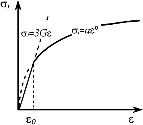
It is supposed that materials obey the law of linear elasticity (2) under elastic strain, and the power law (3) under plastic strain, which are written in the invariant form (see Fig. 1) as
 $${\sigma _{\rm{i}}} = 3G\varepsilon {\rm{,}}\quad (\varepsilon \,\le\, {\varepsilon _0})\quad {\rm{,}}$$
 $${\sigma _{\rm{i}}} = {\sigma _{\rm{s}}} = a{\varepsilon ^b}{\rm{,}}\quad (\varepsilon > {\varepsilon _0})\quad {\rm{,}}$$
where 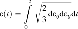 $\varepsilon (t) = \int\limits_0^t {\sqrt {{2 \over 3}{\mathop{\rm d}\nolimits} {\varepsilon _{ij}}{\mathop{\rm d}\nolimits} {\varepsilon _{ij}}} } {\mathop{\rm d}\nolimits} t$ is the amount of strain;
 ${\mathop{\rm d}\nolimits} {\varepsilon _{ij}} = {\mathop{\rm d}\nolimits} \varepsilon _{ij}^{\rm{e}} + {\mathop{\rm d}\nolimits} \varepsilon _{ij}^{\rm{p}}$;
 ${\mathop{\rm d}\nolimits} \varepsilon_{ij} {\rm{,}}\;{\mathop{\rm d}\nolimits} \varepsilon _{ij}^{\rm{e}}{\rm{,}}\;{\mathop{\rm d}\nolimits} \varepsilon _{ij}^{\rm{p}}$ are total, elastic, and plastic strain tensor increments, respectively;
 ${\varepsilon _0}$ is the amount of strain such that the material transforms into a plastic state, the value of
 ${\varepsilon _0}$ is found as the zero solution of the system of Eqs. (2) and (3); G is the modulus of shearing related to Young's modulus E and Poisson's ratio ν through the expression
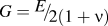 $G = {\raise0.7ex\hbox{$E$} \!\mathord{\left/ {\vphantom {E {2(1 + \nu )}}}\right.\kern-\nulldelimiterspace}\!\lower0.7ex\hbox{${2(1 + \nu )}$}}$; a and b are empirical coefficients.
The strain-hardening diagrams.

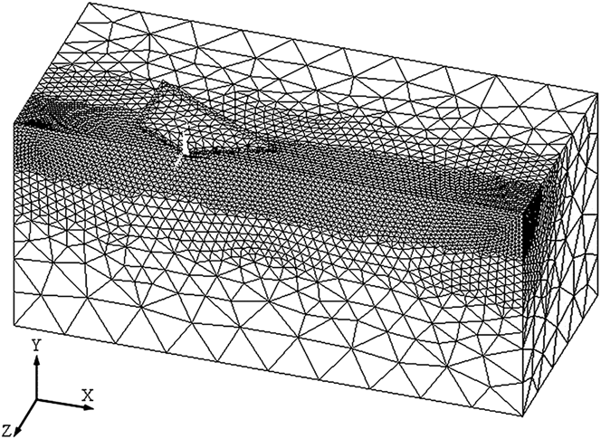
The testing was simulated with the use of the finite element method program ANSYS v.14 on a clustered multiprocessor. To reduce the computations, ½ of a symmetric composition was treated (see Fig. 2). The dimensions of the model of a specimen in the form of a parallelepiped were selected so that the zone of plastic deformation does not reach any face of the parallelepiped during the entire testing, the normal stresses on the faces being lower than 3% of the yield stress. With maximum indentation depth value of 1.4 μm, ½ the size of the indent diagonal, and a scratch length of 6 μm, the dimensions of the specimen model were 15 × 7 × 7 μm. Thus the effect of the specimen dimensions on the simulation results was thereby avoided. The boundary conditions on the specimen were specified in terms of displacements, the lower face was fixed against displacement in all directions, one of the end faces being fixed against horizontal displacements along the x-axis; the symmetry plane of the indenter and the specimen was fixed against displacements along the z-axis. The action of the indenter on the material was set by pressing uniformly on the top end of the indenter. The diamond indenter was viewed as a linearly elastic isotropic material with Young's modulus E = 1140 GPa and Poisson's ratio ν = 0.07.
The finite-element mesh in the initial state.
The strain-hardening diagram determined by Eq. (3) can be with fairly high approximation accuracy described by the MISO material model (multilinear isotropic hardening) from the ANSYS library. Solid 187 3D finite elements with 10 nodes were used to construct a mesh. To ensure a contact between the indenter and the material, an “indenter–body” contact pair was specified, with the lateral surface of the indenter and the body surface penetrated by the indenter being the contacting elements. The friction on the interface was given in the form of the Coulomb law,
 $$\tau = \mu p\quad {\rm{,}}$$
where τ is friction stress, μ is friction factor, p is normal contact pressure.
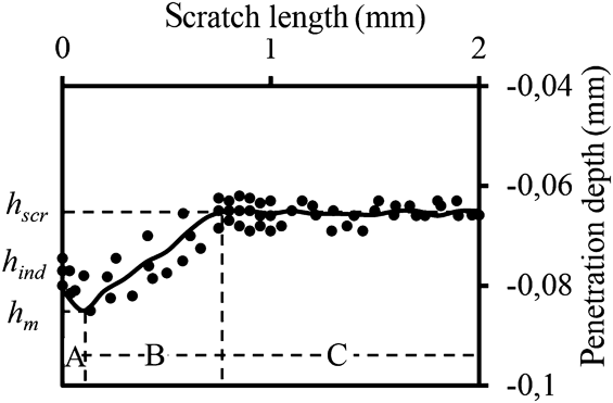
To verify the adequacy of the finite-element model, experiments on the indentation and scratching of pure copper specimens by a Berkovich indenter were made. The choice of verification testing experiments was based on the fact that, when tests are conducted on a microscopic level and lower, fundamental complications arise from the impossibility of making specimens to perform standard mechanical tension and compression tests required for a correct determination of the strain-hardening diagram whose accuracy governs the simulation results. Besides that, uncontrollable result deviations occur in microscopic testing due to the local heterogeneity of the material composition and structure, residual distortions of the near-surface and surface layers caused by machining and incompletely removed by etching etc. Therefore, macroscopic testing was used to verify the model. The scratch experiments were made on the Akashi AVK-HF hardness meter (Akashi, Japan) furnished with a special device for the horizontal motion of the specimen. Ten “edge forward” scratch tests were made under a load of 100 N. A scratch diagram was constructed by the averaged experimental results (see Fig. 3).
The diagram of scratching copper specimens by a Berkovich indenter; the marks symbolize experimental data; the lines represent the simulation results.
The experimental conditions were reproduced in the simulation. The σ–ε diagram, which is necessary for calculations, was obtained experimentally from compression experiments with the same specimens. The mean relative deviations of the experimental and calculated indentation and scratch diagrams did not exceed 5%, and this testifies to the adequacy of the finite-element model.
It is obvious from Fig. 3 that the depth of indenter penetration h into the metal during “edge forward” scratching varies nonmonotonically, with three characteristic portions noticeable on the curve. After the indentation stage is over, the penetration depth is h ind. On the A portion belonging to the beginning of longitudinal shifting, the indenter makes a “plunge”, and the penetration depth increases to the value h m. On the B portion, the indenter “floats” as high as h scr, and the penetration depth stabilizes thereafter on the C portion. The plunge of the indenter on the A portion is attributable to growing pressure р у on the contact surfaces after the beginning of the longitudinal indenter motion. Indeed, the normal force acting on the indenter during indentation is redistributed among all the three indenter faces contacting with the material. At the initial moment of horizontal indenter motion, loading force is redistributed between two faces thus causing an increase in the contact pressure component р у, and hence an increase in the penetration depth.
On the other hand, as the indenter moves longitudinally, the resistance of the environment grows in this direction, and this causes an additional “upthrust” tending to be offset by indenter elevation on the B portion. The penetration depth becomes stable as soon as the balance of forces is achieved on the C portion. The effect discussed is similar to the well-known phenomenon of gliding in motion in a liquid. Indenter “floating” is intensified due to the peculiarity of the formation of pile-ups during longitudinal indenter shifting. The same way as with indentation, a relief results in some decrease in the scratch depth due to the elastic aftereffect.
When the “edge forward” scratching with a Berkovich indenter is effected, the displaced metal is predominantly concentrated in the side pile-ups, whereas it is accumulated in the side pile-ups and in front of the indenter in “face forward” scratching. The piling-up process in front of the indenter when scratching is effected by the “face forward” scheme is instable: the growing pile-up causes indenter “floating”, though the contact area decreases and р у increases, and this makes the indenter plunge again. The process is then repeated thus causing periodic changes in the plunge depth. In the “edge forward” scratching, this process is less pronounced, the indenter vibrations being hardly noticeable. Note that, when simulating “face forward” tests, we encountered difficulties with the stability of the solution process because of a bad distortion of the geometry of the finite elements in the pile-up zone in front of the indenter. It stopped the solution at certain combinations of test parameters and material properties.
III. A “STRESS–STRAIN” DIAGRAM DETERMINATION PROCEDURE
To determine meaningful factors affecting the indentation and scratch diagrams, a numerical experiment was made, with the variation of Young's modulus E = 100–250 GPa, Poisson's ratio ν = 0.3–0.45, the friction factor μ = 0–0.2, which corresponds to the conditions for performing testing of ductile metal materials. The effect of the factors was estimated by the variation of the numerical coefficient C in quadratic approximation generally used for the description of indentation diagrams,
 $$P = C{h^2}\quad {\rm{,}}$$
where P is the load on the indenter; h is penetration depth.
The simulation has shown that the variation of E and ν in the above-mentioned range causes a not more than 0.6% change in C and a 2.2% change in the friction factor μ. This is less than the deviations caused by experimental errors, therefore these factors were not taken into consideration in the development of the procedure. In all further calculations, it was assumed that E = 125 GPa, ν = 0.35, μ = 0.1.
Another important factor affecting the indentation diagrams is the indenter tip curvature radius R, although this effect is known to decrease as the indentation depth increases.Reference Bouzakis, Michailidis, Hadjiyiannis, Skordaris and Erkens12–Reference Pelletier, Krier, Cornet and Mille14
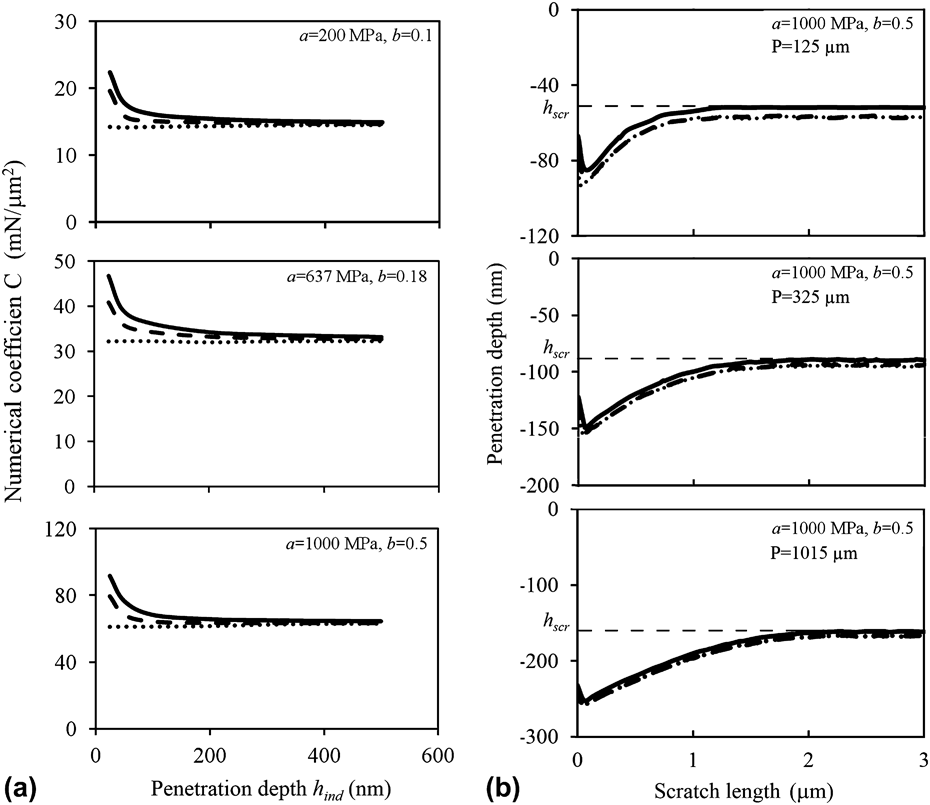
The minimum indentation depth required for the effect of R to be neglected was to be determined. The calculations have been made for the extreme combinations (a = 200 MPa, b = 0.1 and a = 1000 MPa, b = 0.5) and an average combination (a = 637 MPa, b = 0.18) of the coefficients a and b in the power law of hardening which are characteristics of ductile metal materials, see Fig. 4(a). The geometry of the rounded indenter tip was presented as recommended in Ref. Reference Pelletier, Krier, Cornet and Mille14. The indentation diagrams were calculated for indenters 50 and 100 nm in radius and for a sharp indenter (R = 0). The effects of the factors were estimated by the value of C in the quadratic approximation (5), which was calculated when the penetration depth h was changed from 0 to the current value. It is obvious from Fig. 4(a) that the value of C differs considerably in the region of small penetration depths for indenters with rounded tips and sharp ones. As the penetration depth increases, the material surface portion contacting with the rounded indenter tip decreases, thus reducing the effect of the curvature radius. It can be considered that the indenter radius R = 50 nm has a tangible effect on the indentation diagram when h ind < 150 nm, therefore the actual indenter tip geometry may be neglected in the interpretation of experimental results when h ind > 150 nm. When R = 100 nm, the depth is 250 nm.
The variation of the numerical coefficient C in Eq. (5) with the increasing penetration depth h ind (a). The change of the penetration depth for scratching with various loads P on the indenter (b). The indenter radius: 100 nm (—); 50 nm (– –); a sharp indenter (⋅⋅⋅⋅).
Figure 4(b) shows a change in the penetration depth for scratching with various radii R. The curves in Fig. 4(b) are shown for the constant values of a = 1000 MPa and b = 0.5 and various loads P on the indenter. As evident from Fig. 4(b), the effect of the radius R on the depth h scr is tangible only when h ind < 100 nm. Therefore, in the stage of scratching, an increase in the radius R has a smaller effect on the current penetration depth h scr as compared to h ind.
To find the two unknown empirical coefficients in Eq. (3) we proceeded from the fact that it is necessary to have at least two independent experiments. Indentation and “edge forward” scratching with a Berkovich indenter were selected, the load on the indenter being the same.
The parameters h ind and h scr were selected as test characteristics (see Fig. 3) in testing with a maximum load of 5 mN on the indenter. This load is in the operating range for the majority of serially produced nanomechanical test systems. The independence of h ind and h scr results from the following. The tests are performed with a constant vertical force on the indenter, therefore the indenter penetration depths h ind and h scr are governed by the strain hardening of the specimen, and, since the average amount of strain during indentation differs from that in the steady stage of scratching, these values correspond to different points on the stress–strain diagram. The simulation of the test process has shown that the value of h m varies practically proportionally to the value of h ind, therefore it is ill-posed to use it as an independent parameter when determining the σ–ε diagrams.
To relate the test parameters to the coefficients in Eq. (3), computational experiments with a sharp Berkovich indenter were made by the above-discussed finite element model. In the calculations, the coefficients varied in the range typical of ductile metal materials with a = 200–1000 MPa with a step of 100 MPa; b = 0.1–0.6 with a step 0.1. The values of the elastic constants for the material and the indenter were assumed as E = 125 GPa, ν = 0.35 and E = 1140 GPa, ν = 0.07, respectively. The friction factor μ = 0.1 in (4) was assumed. The above-described finite-element model with a sharp-tip indenter was used for calculations. To obtain indentation and scratch diagrams, 34 variants of 3D simulation were made for each process.
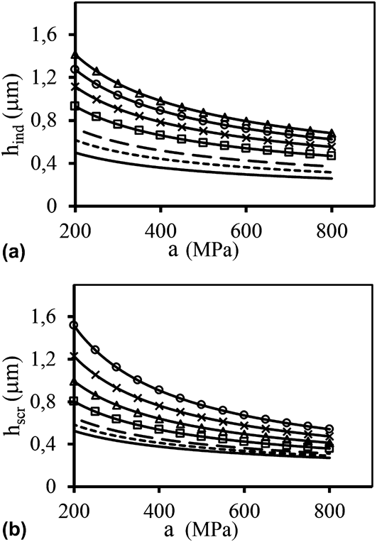
The simulation has yielded the necessary amount of calculation data on h ind and h scr. From these data we have built a diagram of the depth of the penetration and the depth of the scratch of indenter depending on the values of coefficients a and b (see Fig. 5). Note that the indenter penetration depth exceeds 250 nm in all the instances, therefore the calculation results hold true for indenters with dulled tips, too.
The diagrams connecting the depth of penetration of Berkovich indenter (a), scratching by the edge forward (b) versus the empirical coefficients a and b in Eq. (3). Normal load on the indenter is 5 mN. —, b = 0.1; ⋅⋅⋅⋅, b = 0.15; – – , b = 0.2; □, b = 0.3; Δ, b = 0.4; ×, b = 0.5; ○, b = 0.6.
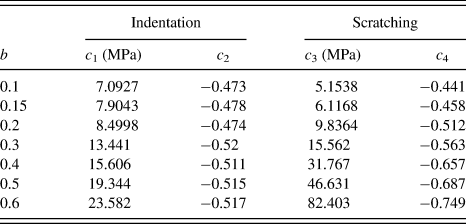
A statistical analysis has shown that, with the approximation confidence R 2 > 0.997, the partial dependences h ind(a) and h scr(a) (see Fig. 5) at fixed values of b are described by power functions of the form
 $${h_{{\rm{ind}}}} = {c_1}{a^{{c_2}}},\quad {h_{{\rm{scr}}}} = {c_3}{a^{{c_4}}}\quad ,$$
where c 1 … c 4 are approximation coefficients and their values are shown in Table I.
The values of approximation coefficients in Eq. (6).
The proposed procedure for determining strain-hardening diagrams described by Eq. (3) is as follows. Experiments on indentation and “edge forward” scratching with a Berkovich indenter are performed on specimens with prepared surfaces under a fixed load of 5 mN. To minimize the effect of a random change in the mechanical properties and the surface relief of the material portion under study, it is desirable to make 15 to 20 measurements, the results being then averaged. Then, the value of h ind known from the experiment, coefficients c 1 and c 2 corresponding to different values of b from Table I, the values of a are determined by the formula
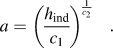 $$a = {\left( {{{{h_{{\rm{ind}}}}} \over {{c_1}}}} \right)^{{1 \over {{c_2}}}}}\quad {\rm{.}}$$
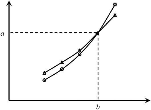
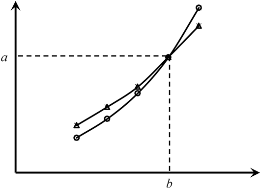
The set of a(b) values arrived at represents possible combinations of the coefficients in Eq. (3) that meet the conditions of the experiment. The dependence a(b) is described analytically or graphically. The same algorithm is used to determine the dependence a(b) satisfying the result of the experiment on the determination of h scr. Then the intersection of the two curves (see Fig. 6) will determine the required pair of values of the coefficients a and b.
Diagrammatic determination of empirical coefficients in the power law of hardening (3): indentation (○), scratching (Δ) (see the explanations in the text).
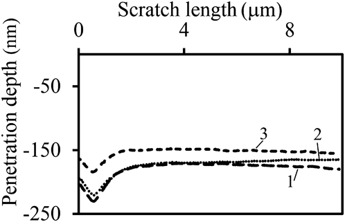
The technique was verified on various metals. The results of studying the surface of the 80%Fe15%Cr5%Al foil are discussed below as an example. Aluminum content was increased to 7 and 13 mass% by gas-phase thermodiffusion aluminizing in a sealed chamber with controlled atmosphere. The specimens were electrolytically polished to avoid the influence of the hardened layer resulting from the preparation of the metallographic specimens. The testing was performed with the use of a Hysitron TI900 (Hysitron, Inc., Eden Prairie, MN) versatile complex designed for nanomechanical testing. The indenter tip curvature radius R ≈ 50 nm. Average plots of penetration of the Berkovich indenter into the foil during scratching with a load of 5 mN on the indenter are given in Fig. 7. The averaging was made over the results of 15 measurements on each material.
Average plots of penetration of the Berkovich indenter into the 80%Fe15%Cr5%Al foil during scratching with a load of 5 mN (aluminum content: 1–5%; 2–7%; 3–13%).
One of the AFM images of indents and scratch on the 7%Al foil after tests with a load of 5 mN is given as an example in Fig. 8.
AFM images of indents and scratch on the 7%Al foil after tests with a load of 5 mN.
The investigation results are shown in Table II. Due to some instability of the experimental data caused by the natural inhomogeneity of the mechanical properties of the alloys, the values of h ind and h scr were averaged over all the experiments. Table II shows the mean values of h scr determined on the interval L = 3.5–5 µm where the experimental values of h scr were the most stable. It does not seem feasible to make fractions-of-micrometer-sized specimens from metal surface layers and test them for tension or compression to verify the σ–ε diagrams obtained. Therefore, comparison calculations were made with the use of Tabor's formula H = Cσr, which involves material flow stress σr at some representative strain εr. Thus, knowing the value of hardness H from the experiment, one can determine one point on the strain-hardening diagram. Of course, Tabor's formula is approximate, semi-empirical. Besides, in the literature, there is no unified opinion about the value of representative strain εr (according to different works, it ranges between 0.056 and 0.11). However, apparently, it can be used for a qualitative estimate of the reliability of the technique developed. In the calculations by Tabor's formula it was assumed that C = 3 on the basis of the data found in Ref. Reference Fedosov and Pešek15 and that εr ≈ 0.08.Reference Tabor10,Reference Johnson16,Reference Milman, Galanov and Chugunova17 For comparison, Table II presents the values of σs calculated by Eq. (3) using the values of a and b obtained for ε = 0.08. The closeness of the results evaluated by 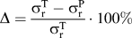 $\Delta = {{\sigma _{\rm{r}}^{\rm{T}} - \sigma _{\rm{r}}^{\rm{P}}} \over {\sigma _{\rm{r}}^{\rm{T}}}} \cdot 100\%$ enables the technique to be recommended for practical applications.
Investigation results for the Fe–Cr–Al alloy.
IV. CONCLUSION
A technique has been developed for the determination of coefficients in the power approximation of the σ–ε diagram by results obtained from tests for scratching with a Berkovich indenter under a normal load of 5 mN on the indenter. The technique is intended for application on nanomechanical testing equipment enabling one to perform tests with recording of loading diagrams in terms of the “normal force – indenter displacement”. To obtain correct results, one must follow the restrictions: indenter penetration depth h ind > 150 nm with the indenter tip curvature radius R < 50 nm and h ind > 250 nm with 50 < R < 100 nm; the tested metal must be ductile enough, for a scratch to be formed by the mechanism of plastic deformation rather than fracture. Our experience has shown that the proposed technique is limitedly applicable to materials suffering phase transformations under deformation (e.g., TRIP-steels) and inapplicable to materials whose indentation diagrams behave intermittently, e.g., Armco iron. If necessary, similar procedures can be developed for other loads on the indenter, the above-mentioned restrictions being imperative to ignore indenter tip dulling.
ACKNOWLEDGMENTS
This work was done according to Program of UB RAS (Project No 12-T-1-1010) and grant of RFBR (Project No 13-08-96061).