1. Introduction

Valley glaciers have some finite surface area and, therefore, must also have some finite length and width. What is less apparent is the relationship between width and length as glaciers get longer. If a glacier is long and sinuous, such as Columbia Glacier, Alaska, does the average width increase with the total length of the glacier or does the Width stay relatively constant? For ice caps and ice sheets, assuming a constant width would be inappropriate. As roughly circular objects which are not constrained by bedrock topography, the width and the length are expected to scale identically. Certainly, the ice dynamics do not favor one direction over another, so there is no dynamical reason to expect that the length and width of an ice cap or a valley glacier will scale differently. However, valley glaciers are constrained by long valley walls which were typically formed as part of some pre-existing river-drainage basin. Variations in the valley geometry make a measurement of a characteristic width (e.g. the mean glacier width) subjective and difficult. The question, then, is what appropriate characteristic value should be selected for glacier widths and how should this value be measured.

Many different analyses, ranging from response-time estimates to volume-area scaling rely on some type of assumption regarding the characteristic width of glaciers e.g.Reference Nye,Nye, 1965; Reference Paterson,Paterson, 1972: Reference Johanncsson,, Raymond,, Waddington, and Oerlemans,Jóhannesson and others, 1989, p. 349; Reference Bahr,, Meier, and Peckham,Bahr and others, 1997). These assumptions span from widths controlled by parabolic channel cross-sections to widths scaling identically to length. Many studies assume that the valley-glacier width does not change with the length and is constant to a reasonable approximation (e.g. Reference Paterson,Paterson, 1994, p. 320). The typical justification is that, for very steep valley sidewalls, the ice is constrained to grow thicker and longer bm not wider. As an irrelevant scaling constant, the width is then removed from the analysis. If, as is often the case, the analysis is intended to apply to more than one glacier, then removing the charactcristic width from a scaling analysis is equivalent to saying that all glaciers have the same characteristic width. This was certainly not the intended result.

To prevent misapplications of the characteristic glacier width, to elucidate the relationship between glacier shapes and valley shapes, and to refine future estimates of response time and volume-area scaling, it is worthwhile to revisit carefully the assumptions regarding length and width scaling. Iu this paper, we examine some of the available valley-glacier data from Europe and Asia and estimate an appropriate sealing relationship. The data suggest that width scales, as length raised to an exponent of 0.6, give a value which is intermediate between the commonly assumed constant widths of valley glaciers and the linear length-width relationship of ice caps and ice sheets.

2. Observations

The World Data Center A for Glaciology and the National Snow and Ice Data Center (NSIDC) have made available digital inventories of 24 476 Eurasian glaciers and ice caps (covering all of the former Soviet Union and the Huang He region of China), and 5422 glaciers from the European Alps. The data for each glacier contain roughly 36 different geometric attributes, ranging from total surface area, mean width and volume to ablation area, snow-line elevation and accuracy estimates of the measurements. The glaciers are classified according to type (e.g. ice cap, valley glacier or glacieret) and other known characteristics of the terminus (e.g. calving vs piedmont), longitudinal profile (e.g. regular vs hanging), and source of nourishment (e.g. snow vs avalanches). A description of the data format and definitions of the terms have been given in Unesco/IAHS (1970) and maps of the general glacier locations in the Eurasian inventory are available from NSIDC.

This analysis is restricted to the length width behavior of mountain and valley glaciers without calving, and without hanging or discontinuous longitudinal profiles. Known surging glaciers were eliminated from the data set. Measurements of thickness and surface area, which were estimated (by the individuals who collected the data) to be less than 95% accurate, have also been removed. Data from the Tarim region of the Eurasian inventory were evaluated separately because of oddities in the data discussed below. This leaves 303 glaciers in the Eurasian inventory and 112 glaciers in the Alps inventory.

For each glacier, five attributes were extracted from the data and used in the following analyses: mean width, maximum length, total area, ablation area and mean depth. Mean width and maximum length were used for direct estimates of the length-width scaling exponent. The total area, ablation area and mean depth measurements were used to give alternative estimates of the width-length relationship. The large number of glaciers (303) with high-accuracy mean depth measurements in the Eurasian inventory seems unreasonable and, therefore, were not used extensively in the following derivations. (Some explanations and implications of the depth measurements are discussed below.) For the Alps inventory, ablation areas are not available, so the length of the ablation area was instead selected from the data.

3. Analysis

Each glacier’s mean width, maximum length, total area, ablation area, ablation length and mean depth are assumed to be characteristic values for that glacier. Characteristic values are single numbers which are representative of the overall behavior of each glacier parameter. Typically, a characteristic value can be measured as several different quantities. For example, the characteristic width could be the mean width (as assumed here), the maximum glacier width or the width at the equilibrium line. The characteristic length could be the maximum length (as assumed here) or the average length along a flowline. In geometric scaling analyses, such as the one presented here, the exact choice of characteristic values is not critical, because each type of characteristic measurement is typically related by additive constants or constants of proportionality. More details on the choice of characteristic quantities can be found in Reference Bridgeman,Bridgeman (1963), Reference Welty,, Wicks, and Wilson,Welty and others (1984) and others.

The relationships between characteristic quantities are typically given by power laws (Reference Schmidt, and Housen,Schmidt and Housen, 1995). This is in part because of the Buckingham Pi theorem, which dictates the construction of non-dimensional quantities which describe a physical problem: these quantities always involve powers of the appropriate variables. We can expect, therefore, that the characteristic length [x] and characteristic width [w] of glaciers will be related by a power law of the form

(1)

for some scaling constant q. Throughout the text, we will use square brackets to indicate characteristic quantities.

Simple geometric arguments also suggest that the length and width of a glacier should be related by a power law. Assume for the moment that each glacier sits in a valley with a shape given by a parabola, cubic or some other simple polynomial of order p. Most valley glaciers are thought to occupy roughly parabolic channels (e.g. Reference Harbor,Harbor, 1992). If the channel has a uniform cross-section, then ice will fill the valley to some depth h. Therefore, as a low-order approximation,

(2)

Scaling analyses by Reference Bahr,, Meier, and Peckham,Bahr and others (1997) show that the characteristic thickness of a glacier scales with the characteristic lenglh as

(3a)

for steep surface slopes, and

(3b)

for shallow surface slopes. These relationships are not derived using any assumption about glacier w idth. The exponent n comes from Glen’s flow law relating stress and strain rates (

From Equations (2) and (3),

(4)

for steep slopes, and from Equations (2) and (4),

(5)

for shallow slopes. In other words, for characteristic length width scaling, Equations (4) and (5) suggest a power-law form winch is equivalent to Equation (1).

3.1. Area-length data

If characteristic length and width are related by a power law, then a regression on a log-log plot of mean glacier width vs maximum glacier length will give the scaling exponent q Equation (1)). However, mean width measurements are very subjective and the available data show a “shotgun” scattering of data points (Fig. 1). Instead of using mean width, the easily and frequently measured glacier-surface area, S, can be used instead. The surface area is proportional to the glacier length times the width, so

(6)

by Equation (1). A linear regression of log[S] vs log[x] will give q + 1. For the Eurasian inventory, q = 0.61 with a squared correlation coefficient of R ² = 0.81 (Fig. 2a). For the Alps, q = 0.69 and R ² = 0.89 (Fig. 2b).

3.2. Volume-area data

The plots of [S] vs [x] in Figure 2 clearly show that q > 0. However, while q ≈ 0.6 gives the best fits, q = 1 (the same as ice caps) still gives reasonable appearing fits (Fig. 3). To help pin down an accurate value, an independent estimate off q is possible by plotting glacier volumes vs surface area. Using arguments from Reference Bahr,, Meier, and Peckham,Bahr and others (1997)

(7)

where

(8)

for steep slopes, and

(9)

for shallow slopes. Volume measurements are not provided in the inventories but, using reported values of the mean depth from the Eurasian data set, a regression of [S][h] vs [S] gives γ = 1.36 with R ² = 0.996 (Fig. 4a). Regressions made with different data sets show that γ ≈ 1.36 (Reference Chen, and Ohmura,Chen and Ohmura, 1990; Reference Bahr,, Meier, and Peckham,Bahr and others, 1997), so the estimate from the Eurasian inventory appears reasonable; but while volume-area plots are expected to be significantly less noisy than area-length plots (see Appendix), the near-absence of scatter in the Eurasian data seems unrealistic. The large number of available mean-depth measurements is also suspect (such measurements are difficult to make).

Fig. 1.

Length vs width for (a) Eurasian data and (b) Alps. (Log-log versions of these plots do not help to elucidate any power-law scaling trend in the data.)

Fig. 2.

Log-log plot of surface area vs length for (a) Eurasia with linear regression log[S] = 1.61 log[x]-0.88, R² = 0.81, and (b) Alps with log[S] = 1.69 log[x]-0.96, R² = 0.89.

Fig. 3.

Log-log plot of surface area vs length for (a) Eurasia with regression [S] = 0.18[x]², R² = 0.64, and (b) Alps with [S] = 0.28[x]², R² = 0.88. Note that the slope of the regression line has been fixed by the exponent 2, and the coefficients of 0.18 and 0.28 determine the spatial position of the line. For the Eurasian plot, the large glaciers pull the regression below the bulk of the data.

In the Alps inventory, all of the 112 glaciers (whose selection criteria have been described above) purport to give mean-depth measurements. A plot of [S][h] vs [S] for the, Alps inventory shows an unusual split (Fig. 4b); a regression on the smaller glaciers gives γ = 1.25 and a regression on the larger glaciers gives γ = 1.40. The value γ = 1.25 is considered unreasonable except for ice caps, while γ = 1.40 is consistent with other vloume-area measurements in the Alps (Reference Meier, and Post,Meier and Bahr, 1996). As with the Eurasian data set, the lack of noise and the large number of available measurements is unrealistic. Furthermore, the split in the data set appears artificial and suggests that the mean depths were Calculated rather than measured.

It is possible that some or all of the mean depths reported in the Eurasian and Alps inventories have been calculated using previously published empirical volume-area results (e.g. from Reference Chen, and Ohmura,Chen and Ohmura (1990), Reference Kuz’michenok,Kuz’michenok (1996) and references within) or from simple estimates assuming constant basal shear. Regardless of the source of [h], enough independent studies (e.g. Reference Macheret., Cherkaaov, and Babrova,Macheret and others, 1988: Reference Chen, and Ohmura,Chen and Ohmura, 1990: Reference Meier, and Bahr,Meier and Bahr, 1996) have concluded that γ ≈ 1.36−1.40, that those values (and those in Figure 4) are reasonable for estimating q. From Equations (8) and (9),

(10)

for steep slopes, and

(11)

for shallow slopes. The exponents γ and n are known, so q can be determined for any selected value of m.

Fig. 4.

Log-log plot of volume vs area for (a) the Eurasia data with regression log[V] = 1.36 log[S] + 3.70 and R² = 0.996, and (b) the Alps data. The smaller glaciers in the Alps data have a regression log[V] = l.25log[S] + 2.21 (R² = 0.99), and the larger glaciers have a regression log[V] = 1.40log[S] + 3.00 (R² =0.99).

A value for m can be estimated using ablation-area measurements from the Alps and Eurasian data inventories. Reference Bahr,, Meier, and Peckham,Bahr and others (1997) have shown that the ratio of an accumulation area to the area of an entire glacier is given by

(12)

Ablation areas and total surface areas give an AAR estimate for each glacier in the Eurasian inventory; the length of the ablation area and the maximum lenglh of each glacier give an estimate of each glacier’s AAR in the Alps inventory (assuming constant width). For the Eurasian glaciers, the average AAR is 0.577 (with a standard deviation of 0.112), and for the Alps the average AAR is 0.580 (with a standard deviation of 0.110). Using Equation (12), the exponent m is then estimated to be 1.99 for the Eurasian glaciers and 2.04 for the Alps. Note that, with a standard deviation of ±0.112, the estimates for m can range from roughly 0.7 to 4.7. However, AARs are a noisy function of time and space and must be observed precisely at the end of the balance year. As a result, the mean value of hundreds of measurements is the most reliable approximation of the AAR (e.g. Reference Meier, and Post,Meier and Post, 1962; Reference Dugdale,Dugdale, 1972) and the most reasonable value with which to estimate m.

For n = 3 and for the observed values of γ ≈ 1.36 (Fig. 4) and m ≈ 2 (from the mean AAR), Equations (10) and (11) predict q = 0.6 for steep slopes and q = 1.0 for shallow slopes. Small changes in the values of γ and m also give values of q near 0.6 or 1.0. If m ranges over 0.7-4.7 (from the standard deviation of the AAR), then q for steep slopes can vary from roughly 0 to 2.1 and q for shallow slopes can vary from roughly 0.6 to 2.0. Although the range of possible values for the AAR, m and q can be quite large, volume-area scaling estimates of q = 0.6 using the more reliable mean value of the AAR lends at least some support to the conclusions from the area-length data. Most valley glaciers in Eurasia and in the Alps are expected to have relatively steep surface slopes and the sleep-slope estimate of q = 0.6 shows a good agreement with the area-length data estimates of q = 0.56 (Eurasia) and q = 0.69 (Alps).

4. Discussion

A previous study on the network geometry of six large Alaskan glaciers (Columbia, Knik, Russell, Harvard, Barnard and Matanuska Glaciers) has suggested that glacier area is related to the longest channel length with an exponent of roughly 2.0 (Reference Bahr, and Peckham,Bahr and Peckham, 1996). In other words, from Equation (2), q ≈ 1.0 for these six glaciers. Although six glaciers are a small and not necessarily representative sample, their slopes are small less than approximately 3° on average), and q = 1 may be appropriate, as explained above. In general, however, there are far more small-sized and steep-sloped valley glaciers than large-sized and shallow-sloped valley glaciers in any mountainous region of the world. For mountain and valley glaciers, the length width exponent of q ≈ 0.6 should be more generally applicable than the exponent q = 1.0.

Based on the simple geometrical motivation of Equation (4), the characteristic width for steep-sloped glaciers should be related to the characteristic length by an exponent q = m +1/p(n + 2). In other words,

(13)

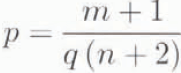
and for q = 0.6, n = 3 and m = 2, this implies that p = 1.0. In this case, the characteristic glacier width is linearly related to the characteristic glacier thickness (Equation (2)).

Note that, because p has been derived using characteristic values, this implies [w] ∝ [h]. This is not the same as w #x221D;h. In fact, w #x221D;h implies [w] ∝ [h], but the inference is one-way only. Characteristic values can be derived from relationships between variables but the far more general relationship between variables cannot be derived from the reduced information contained in the characteristic numbers (imagine, for example, trying to derive the Navier-Stokes equations from the Reynolds number). So, although p = 1, this does not mean that glacier valleys have the V-shaped cross-section implied by w #x221D; h.

Nonetheless, because glacier valleys have roughly parabolic cross-sections, a value closer to p = 2 is expected. For q = 0.6, this would imply m = 5.0, and from Equation (12), AAR = 0.699. While this AAR is not improbable, it is over one standard deviation off of the mean AAR = 0.58 ± 0.11 observed for both the Alps and Eurasian inventories. Therefore, the exponent p is almost certainly smaller than p = 2 and probably close to the value p = 1 predicted from the mean AAR.

It is difficult to imagine circumstances which would give the well-known parabolic glacier channels (w ∝ h ^½), yet lead to a linear relationship between characteristic glacier length and characteristic width, (w ∝ h ^½) is true for the valley cross-section, then [w] ∝ [h]^½ is also true for the valley. The only reasonable explanation, therefore, is that the characteristic glacier width and thickness are different from the characteristic width and thickness of the glacier valley. The three-dimensional shape of the actual glacier within the three-dimensional valley must be responsible for the difference. Consider, for example, a channel with a parabolic cross-section (w = kh ^½ and a channel bottom which increases elevation as a parabolic function of longitudinal distance x up the valley. If the channel also necks down linearly with distance toward the valley outlet (k ∝ x), then a glacier (with any power-law longitudinal surface profile) sitting in this valley will have an average width which grows linearly with the length of the glacier (see next paragraph). While this is a somewhat artificial valley geometry, it demonstrates that the characteristic width is not always simply related to the parabolic channel cross-section; and, in fact, this example shows that a parabolic cross-section can be consistent with the linear relationship, [w] ∝ [h].

A whole class of such examples with parabolic cross-sections can be constructed and, with these examples, the length-Width exponents q ≈ 0.6 and p ≈ 1 may give very general information about typical glacier-valley geometries. Assume that all glacier valleys can be suitably described as having parabolic cross-sections which neck down (in the longitudinal direction) as some other power-law function of longitudinal distance, x ^a. Assume that the elevation of the valley bottom changes as another power-law x ^b, and that the glacier sitting in the valley has lenglh L with a longitudinal surface profile described as a power-law x ^c (with c < b so that the ice surface lies above the channel bed). (Such power-law assumptions are restrictive but give reasonable low-order approximations to many realistic geometries.) The characteristic width is then given by

(14)

where L ^b-c x ^c − x ^b gives the ice thickness at any position x (the constant L ^b-c ensures that the glacier bed and the ice surface meet at the head of the glacier x = L). By considering the length scales in Equation (14), we can see immediately that

(15)

where the characteristic length, [x], is defined as the glacier length. Similarly,

(16)

and by considering lenglh scales (or by direct integration),

(17)

Combining Equations (15) and (17) gives

(18)

In other words, 1/p = ½+a/b (Equations (2) and (18)). From the data p ≈ 1, so for glacier valleys, the ratio a/b ≈ ½. Under the stated power-law geometry assumptions, this gives a fairly general restriction on the rate at which glacier vallcys neck down and on the rate at which the bottoms of glacier valleys change elevation. As the longitudinal profile of the glacier channel becomes increasingly concave (large b), the valley must get increasingly “fatter” or “wider” with a distance up the valley (large a). If b ≈ 3/5, as suggested by Equations (3) and (17) (when m = 2 and n = 3), then a = 5/6 which suggests that glacier valleys might neck down almost linearly with distance. Of course, the applicability of power-law geometries is debatable but more importantly than any specifics, this example does demonstrate that there is a large class of valley geometries (having parabolic cross-sections) consistent with [w] ∝ [h].

5. Conclusions

The Eurasian and Alps inventories show that characteristic valley-glacier widths are related to characteristic valley-glacier lengths by [w] ∝ [h]^q with q ≈ 0.6. This exponent is significantly different from both the linear relationship observed for large ice caps and the constant widths sometimes hypothesized for valley glaciers. The scaling exponent 0.6 is derived from observations of area-length scaling and is supported by observations of volume-area scaling. The volume area observations imply that q = 0.6 is consistent with accumulation-area ratios of slightly less than two-thirds (as frequently assumed and comparatively steep (rather than shallow) surface slopes.

The exponent q ≈ 0.6 implies that characteristic glacier width is linearly related to characteristic glacier thickness. While this might suggest that glaciated and glacierized valleys should be V-shaped, the shape of the glacier can behave differently (though not independently) from the shape of the valley. By allowing changes in channel width with longitudinal distance and variations in the glacier surface profile, glaciers and valleys with a fairly general class of shape can have parabolic cross-sections but a linear relationship [w] ∝ [h].