1. Introduction
In 1763, Richard Price published on behalf of his recently deceased friend, the Reverend Thomas Bayes, a paper that introduced what would become the atomic element of probabilistic inference: Bayes’ rule [Reference Bayes16]. The paper though was widely ignored. About a decade later, the same rule was discovered by Pierre-Simon Laplace and, while Laplace laid its foundations, the theory of inference based on this rule became known as Bayesian inference. So confident was Laplace in the theory that he famously calculated the odds at 11,000 to 1 that the mass of Saturn as determined by a former student was correct to within 1%, 1,000,000-to-1 odds on the mass of Jupiter [[Reference Laplace29], translated from 1825 French edition, pp. 46-47]. (Based on the most recent available data, he would have collected on the bet on Saturn.) Bayesian inference has been used in a great variety of applications from Henri Poincaré’s defense of Captain Dreyfus to Alan Turing’s breaking of the Enigma code [Reference McGrayne34]. In modern day, it provides the crucial framework for inference in such fields as statistics, decision theory, computational neuroscience, machine learning, computer vision, state estimation, and robotics.
The objective common to all these applications is the determination of a posterior probability to test some hypothesis or to calculate some estimate based on prior information and observed measurements. However, it is not always possible to find the posterior exactly. Indeed, we must often resort to approximate techniques. One such technique, which will occupy us here, is that of variational inference or variational Bayes [Reference Bishop17]. In this variational approach, the goal is to find the probability density function (PDF) that comes closest to the posterior as determined by minimizing a loss functional subject to the constraint that the distribution sought be drawn from a tractable class of densities, for example, where the posterior has to take the form of a Gaussian distribution. A common choice for the loss functional is the Kullback-Leibler (KL) divergence [Reference Amari5, Reference Barber8, Reference Bishop17, Reference Blei, Kucukelbir and McAuliffe18, Reference Csiszár20, Reference Hinton and van Camp25, Reference Jordan, Ghahramani, Jaakkola and Saul27] although others such as Bregman [Reference Adamčík1, Reference Painsky and Wornell36], Wasserstein [Reference Ambrogioni, Güçlü, Güçlütürk, Hinne, Maris and van Gerven7], and Rényi divergences [Reference Li and Turner30] have been used.
The field of variational inference based on the KL divergence is already well trodden although the research is hardly exhausted. The chosen class of densities from which the approximate posterior is to be shaped is key to variational inference. In the mean-field approximation, for example, the solution to the minimization of the divergence is constructed as a product of densities from a chosen family of admissible functions such as a Bayesian mixture of Gaussians [Reference Bishop17]. Another possibility is using Bayesian mixtures of exponential families [Reference Amari5, Reference Wainwright and Jordan44]. A number of algorithms by which to execute the minimization exist including the variational EM algorithm, natural gradient descent, and Gaussian variational inference.
In [Reference Jordan, Ghahramani, Jaakkola and Saul27], it is observed that “there is not as yet a systematic algebra that allows particular variational transformations to be matched optimally to particular graphical models.” While this was written two decades ago and specifically about graphical models, the remark finds resonance in the present work.
In previous work [Reference Barfoot, Forbes and Yoon14], we developed a practical robotic state estimation tool based on variational inference and compared it to maximum a posteriori (MAP), showing some advantages in certain situations. For example, the method we developed, dubbed Exactly Sparse Gaussian Variational Inference, can be used to solve the famous simultaneous localization and mapping (SLAM) problem. The current paper shows this existing method can be viewed through a different lens, that of iterative projections in a special space known as a Bayesian Hilbert space or Bayes space for short [Reference van den Boogaart, Egozcue and Pawlowsky-Glahn43]. The primary contribution of this paper is therefore to make this connection between two quite different fields and hopefully to open the door to future extensions.
Our aim is to introduce a kind of information algebra to variational inference that not only provides a convenient and effective framework for analysis but also reveals key relationships to past work. This algebra has its origins in the work of [Reference Aitchison2] on compositional data in statistics. Compositional data can be represented on a simplex as with probability distributions for a finite set of discrete events. The resulting Aitchison geometry or Aitchison simplex establishes a vector space, in which vector addition is a normalized multiplication (perturbation) and scalar multiplication is a normalized exponentiation (powering). With an appropriate inner product, the set of PDFs over a finite discrete space was formalized as a Hilbert space by [Reference Pawlowsky-Glahn and Egozcue37] and independently investigated by [Reference Barfoot9] and [Reference Barfoot and D’Eleuterio12] in their stochastic algebra. The extension to continuous variables was first published by [Reference Egozcue, Diaz-Barrero and Pawlowsky-Glahn23] and also studied by [Reference Barfoot and D’Eleuterio13] for the case of finite domains. The generalization to include probabilities and measures on the whole real line was made by [Reference van den Boogaart, Egozcue and Pawlowsky-Glahn42, Reference van den Boogaart, Egozcue and Pawlowsky-Glahn43], who introduced the term Bayesian Hilbert space.
In such a space, Bayes’ venerated rule becomes
 \begin{equation} p(\textbf{x}|\textbf{z}) = p(\textbf{z}|\textbf{x})\oplus p(\textbf{x}) \end{equation}
where
 $\oplus$
indicates vector addition. (The normalization inherent in the operations accounts for the marginal
 $p(\textbf{z})$
automatically.) Each new measurement made to refine the posterior becomes one more term added to the sum. It is this linear feature of a Bayesian Hilbert space that makes the structure ideally suited to variational inference.
The set of Gaussians, in an appropriately extended sense, constitutes a subspace of Bayes space as do exponential families. An arbitrary PDF in one of these subspaces can be expressed in the simple and usual manner as a linear combination of a basis for the subspace. The problem of variational inference can thus be expressed as the minimization of a divergence over a set of Fourier coefficients.
The linear-algebraic structure of these spaces affords us a new perspective and provides new insight. We show, for example, that the solution to variational inference based on the KL divergence can be viewed as an iterative projection, in the Euclidean sense, onto a given subspace. Indeed, this algorithm is essentially a Newton-like iteration scheme to solve for the minimum of the divergence, having a form identical to the natural-gradient-descent technique of [Reference Amari4]. Moreover, using a subspace of Gaussians reproduces the recent results of [Reference Barfoot, Forbes and Yoon14].
We also employ an information measure using a norm for Bayes space. This allows for a metric to be defined on the space, which can be interpreted as the distance between two PDFs. A (symmetric and quadratic) divergence between PDFs can be based on the distance metric. It is notable that each step in our iterative projection scheme is a local minimization of this divergence.
While this connection between variational inference and projection in Bayes space is exciting, there are still some open challenges around the approach. In the current formulation, there is no guarantee that our projection scheme will result in a valid PDF, although in practice we find the case to be so quite often, particularly with a good initial guess for the posterior estimate. Throughout we attempt to pinpoint the specific challenges and limitations of our approach so that improvements may follow in future work.
We shall begin with an overview of Bayesian Hilbert spaces in the next section. In Section 3, we discuss subspaces and bases, including exponentiated Hermite polynomials and Gaussian distributions. The variational inference problem for the KL divergence as viewed from the purchase of a Bayesian Hilbert space is considered in Section 4. The specific case of using a Gaussian subspace, that is, Gaussian variational inference, is treated in Section 5. Discussion is provided in Section 6 and we end with a few concluding remarks.
2. Bayesian Hilbert spaces
Let us consider some domain
 $\mathcal{X}$
for our PDFs, for example,
 $\mathbb{R}^N$
; we shall refer to
 $\textbf{x} \in{\mathcal{X}}$
as the state. A PDF
 $p(\textbf{x})$
assigns a nonnegative, finite value to each element of
 $\mathcal{X}$
such that
 \begin{equation} \int _{{\mathcal{X}}} p(\textbf{x}) \, d\textbf{x} = 1. \end{equation}
It turns out that this condition provides challenges when it comes to defining Bayes space on an infinite domain. As we will see, not all members of Bayes space (as we define it) will be PDFs and not all PDFs will be members of Bayes space; however, there is a large enough intersection between the two sets that Bayes space will be of practical use. Notationally, we will use
 $p(\textbf{x})$
to mean a member of Bayes space throughout, indicating when the member is a valid PDF.
We provide a lightweight explanation of Bayes space, referring to [Reference van den Boogaart, Egozcue and Pawlowsky-Glahn43] for more detail. We define the following set of functions:
 \begin{equation}{\mathcal{B}}^2 = \left \{ p(\textbf{x}) = c \exp ( - \phi (\textbf{x})) \, \biggl | \, 0 \lt c \lt \infty, \int _{{\mathcal{X}}} \phi (\textbf{x})^2 \, \nu (\textbf{x}) \, d\textbf{x} \lt \infty \right \}, \end{equation}
where
 $\nu (\textbf{x})$
is an appropriate measure for
 $\mathcal{X}$
(loosely, a weighting function); we will assume that
 $\nu (\textbf{x})$
is in fact a PDF (and from
 ${\mathcal{B}}^2$
) throughout although this is not necessary. Essentially, each member of
 ${\mathcal{B}}^2$
is an exponentiated function from
 ${\mathcal{L}}^2$
, the set of square-integrable functions under our chosen measure. Importantly, there is no requirement for
 $p(\textbf{x}) \in{\mathcal{B}}^2$
to be a valid PDF; however, if we have that
 $c^{-1} = \int _{{\mathcal{X}}} \exp (\!-\phi (\textbf{x})) \, d\textbf{x}$
, it will be so. Moreover, not all PDFs are members of
 ${\mathcal{B}}^2$
as we do not allow members to take on the value of zero anywhere in the domainFootnote 1, meaning only those PDFs that are strictly positive are contained (e.g., Gaussians and other exponential families).
We say that two members,
 $p_1(\textbf{x}) = c_1 \exp (\!-\phi _1(\textbf{x})), p_2(\textbf{x}) = c_2 \exp (\!-\phi _2(\textbf{x})) \in{\mathcal{B}}^2$
, are equivalent (equal) if and only if
 $\phi _1(\textbf{x}) = \phi _2(\textbf{x})$
; in other words, the normalization constants,
 $c_1$
and
 $c_2$
, need not be the same. Under these conditions, we have that
 ${\mathcal{B}}^2$
is isomorphic to
 ${\mathcal{L}}^2$
.
We define vector addition [Reference van den Boogaart, Egozcue and Pawlowsky-Glahn42],
 $\oplus \;:\;{\mathcal{B}}^2\times{\mathcal{B}}^2 \rightarrow{\mathcal{B}}^2$
, between two elements
 $p_1, p_2 \in{\mathcal{B}}^2$
to be
 $p_1 \oplus p_2$
:
 \begin{equation} (\forall \textbf{x} \in{\mathcal{X}}) \quad (p_1 \oplus p_2)(\textbf{x}) = p_1(\textbf{x})p_2(\textbf{x}) = c_1 c_2 \exp ( - ( \phi _1(\textbf{x}) + \phi _2(\textbf{x}) ) ) \in{\mathcal{B}}^2, \end{equation}
and likewise scalar multiplication [Reference van den Boogaart, Egozcue and Pawlowsky-Glahn42],
 $\,\cdot\,:\; \mathbb{R}\times{\mathcal{B}}^2 \rightarrow{\mathcal{B}}^2$
, of
 $p \in{\mathcal{B}}^2$
by
 $\alpha \in \mathbb{R}$
to be
 $\alpha \cdot p$
:
 \begin{equation} (\forall \textbf{x} \in{\mathcal{X}}) \quad (\alpha \cdot p)(\textbf{x}) =(p(\textbf{x}))^\alpha = c^\alpha \exp ( -\alpha \phi (\textbf{x})) \in{\mathcal{B}}^2. \end{equation}
With these operations,
 ${\mathcal{B}}^2$
is established as a vector space, termed a Bayesian linear space, over the field
 $\mathbb{R}$
[Reference van den Boogaart, Egozcue and Pawlowsky-Glahn42]. Notably, the zero vector
Footnote 2 is simply any constant function,
 $c\exp (0)$
. Vector subtraction [Reference van den Boogaart, Egozcue and Pawlowsky-Glahn42] is defined in the usual way,
 $p_1 \ominus p_2 = p_1 \oplus (\!-\!1) \cdot p_2$
:
 \begin{equation} (\forall \textbf{x} \in{\mathcal{X}}) \quad (p_1 \ominus p_2)(\textbf{x}) = \frac{c_1}{c_2} \exp ( -(\phi _1(\textbf{x}) - \phi _2(\textbf{x}))) \in{\mathcal{B}}^2. \end{equation}
We note that subtraction, or the inverse additive operation, is equivalent to the Radon-Nikodym derivative [Reference van den Boogaart, Egozcue and Pawlowsky-Glahn42].
To turn a member of
 ${\mathcal{B}}^2$
into a valid PDF we define the normalization operator,
 $\,\downarrow \!{p}$
:
 \begin{equation} (\forall \textbf{x} \in{\mathcal{X}}) \quad (\!{\,\downarrow \!{p}})(\textbf{x}) = \frac{p(\textbf{x})}{\int _{\mathcal{X}} p(\textbf{z}) \, d\textbf{z}} \in{\mathcal{B}}^2. \end{equation}
This operation can only be applied to those members of
 ${\mathcal{B}}^2$
that are equivalent to a valid PDF; in other words, it must be that
 $\int _{\mathcal{X}} p(\textbf{x}) \, d\textbf{x} \lt \infty$
. We will refer to the subset of
 ${\mathcal{B}}^2$
whose members are equivalent to a valid PDF as
 $\,\downarrow \!{{\mathcal{B}}^2} \subset{\mathcal{B}}^2$
; note that this subset is not a subspace under our chosen addition and scalar multiplication operators. As a point of order, the normalization operator is not strictly required in the establishment of
 ${\mathcal{B}}^2$
, only when we want to make the connection to a valid PDF.
As mentioned above, Bayes’ rule can be rendered as
 $p(\textbf{x}|\textbf{z}) = p(\textbf{z}|\textbf{x})\oplus p(\textbf{x})$
. The normalizing marginal
 $p(\textbf{z})$
is accounted for in the implied equivalence of the “
 $=$
” operator. We could also write
 $p(\textbf{x}|\textbf{z}) = \,\downarrow \!{(p(\textbf{z}|\textbf{x})\oplus p(\textbf{x}))}$
, which then makes the right-hand side a valid PDF through normalization.
2.1. Inner product
We endow the vector space with an inner product [Reference van den Boogaart, Egozcue and Pawlowsky-Glahn43] defined as
 \begin{equation} \left \langle{p_1},{p_2}\right \rangle = \frac{1}{2} \int _{\mathcal{X}} \int _{\mathcal{X}} \ln \left ( \frac{p_1(\textbf{x})}{p_1(\textbf{y})} \right ) \ln \left ( \frac{p_2(\textbf{x})}{p_2(\textbf{y})} \right ) \nu (\textbf{x}) \, \nu (\textbf{y}) \, d\textbf{x} \, d\textbf{y}, \end{equation}
where
 $\nu (\!\cdot\!)$
is again a density function corresponding to an appropriate measure for
 $\mathcal{X}$
. Notably, we see that because of the way the inner product is defined the normalization constants,
 $c_1$
and
 $c_2$
, associated with
 $p_1$
and
 $p_2$
play no role.
Because
 $\nu$
is a valid PDF, we can also write the inner product in (8) as
 \begin{equation} \left \langle{p_1,}\;{p_2}\right \rangle = \mathbb{E}_\nu \!\left [ \ln p_1 \ln p_2 \right ] - \mathbb{E}_\nu \!\left [ \ln p_1 \right ] \mathbb{E}_\nu \!\left [ \ln p_2 \right ], \end{equation}
where
 $\mathbb{E}_\nu [\cdot]$
is the expectation with respect to
 $\nu$
. To be clear, when we use expectations the argument,
 $f(\textbf{x})$
, and the measure (a PDF),
 $\nu (\textbf{x})$
, are defined over the same space,
 $\mathcal{X}$
:
 \begin{equation} \mathbb{E}_{\nu (\textbf{x})}[f(\textbf{x})] = \int _{{\mathcal{X}}} f(\textbf{x}) \nu (\textbf{x}) \, d\textbf{x}, \end{equation}
although sometimes we will abbreviate this as
 $\mathbb{E}_\nu [f]$
. In this work, we shall always take the measure to be a PDF (and from
 ${\mathcal{B}}^2$
); however, we shall refer to it as the measure to distinguish it from the other densities involved. Following [Reference van den Boogaart, Egozcue and Pawlowsky-Glahn43], then, we can claim that
 ${\mathcal{B}}^2$
with inner product (8) forms a separable Hilbert space, which is referred to as a Bayesian Hilbert space. We shall sometimes briefly refer to it as a Bayesian space or Bayes space.
2.2. Information and divergence
The norm [Reference van den Boogaart, Egozcue and Pawlowsky-Glahn43] of
 $p \in{\mathcal{B}}^2$
can be taken as
 $\|p\| ={ \langle{p},{p} \rangle }^{1/2}$
. Accordingly, we can define the distance between two members of
 ${\mathcal{B}}^2$
,
 $p$
and
 $q$
, simply as
 $d(p,q) = \|p\ominus q\|$
, which induces a metric on Bayes space.
The norm of
 $p$
can be used to express the information content of the PDF (if it is in
 ${\mathcal{B}}^2$
). In fact, we shall define
 \begin{equation} I(p) = \frac{1}{2}\|p\|^2 = \frac{1}{2}\left \langle{p},{p}\right \rangle \end{equation}
as the information
Footnote 3 in
 $p$
. (The reason for the factor of
 $\frac{1}{2}$
will become evident.) As an example, consider
 $p ={\mathcal{N}}(\mu,\sigma ^2)$
(over the domain
 $\mathbb{R}$
) and measure
 $\nu ={\mathcal{N}}(0,1)$
. The information is
 $I(p) = (1+2\mu ^2)/4\sigma ^4$
. The smaller the variance, the larger the information indicating that the PDF concentrates its probability mass more tightly about its mean; that is, we know better where to expect the state so we may say that we have more information about it.
We shall furthermore find it useful to define a divergence between two members of
 ${\mathcal{B}}^2$
,
 $p$
and
 $q$
, as
 \begin{equation} I(p\ominus q) = \frac{1}{2}\left \langle{p\ominus q},{p\ominus q}\right \rangle. \end{equation}
This is the information contained in the difference of
 $p$
and
 $q$
. Unlike the KL divergence, this divergence is symmetric in
 $p$
and
 $q$
and quadratic in Bayesian space. Clearly,
 $p = q$
if and only if
 $I(p\ominus q) = 0$
. Geometrically, the divergence is (half) the squared Euclidean distance between
 $p$
and
 $q$
in Bayes space.
2.3. Stochastic derivative
Accompanying this algebra is a functional calculus. Consider
 $p(\textbf{x}|\theta ) \in{\mathcal{B}}^2$
depending continuously on some parameter
 $\theta$
. We define the stochastic partial derivative of
 $p$
with respect to
 $\theta$
as [Reference Barfoot and D’Eleuterio13, Reference Egozcue, Pawlowsky-Glahn, Tolosana-Delgado, Ortego and van den Boogaart22]
 \begin{equation} \frac{\eth p}{\eth \theta } = \lim _{\lambda \rightarrow 0} \frac{1}{\lambda }\cdot \bigl ( p(\textbf{x}|\theta + \lambda ) \ominus p(\textbf{x}|\theta ) \bigr ). \end{equation}
Note that the result of this operation remains an element in
 ${\mathcal{B}}^2$
. We can also define directional derivatives and a gradient operator, but these will not be required here.
3. Subspaces and bases
While
 ${\mathcal{B}}^2$
is an infinite-dimensional space, it contains infinitely many finite-dimensional subspaces. We can in fact build a subspace
 $\mathcal{Q}$
by taking the span of a set of
 $M$
vectors
 $B = \{b_1,\ldots,b_M\}$
, namely,
 \begin{equation}{\mathcal{Q}} = \text{span}\left \{ b_1, \ldots, b_M \right \}. \end{equation}
If we choose
 $B$
to be linearly independent, it will form a basis for
 $\mathcal{Q}$
. We can accordingly write every vector
 $q$
in
 $\mathcal{Q}$
as a linear combination of
 $B$
, that is,
 \begin{equation} q = \bigoplus _{m=1}^M \alpha _m\cdot b_m, \end{equation}
where
 $\alpha _m \in \mathbb{R}$
are unique. We use the notation
 $\bigoplus _{m=1}^M \alpha _m \cdot b_m$
to mean
 $\alpha _1 \cdot b_1 \oplus \cdots \oplus \alpha _M \cdot b_M$
, paralleling
 $\sum _{m=1}^M$
for normal addition.
As a shorthand, we will denote
 $\textbf{b} = \begin{bmatrix} b_1 & b_2 & \cdots & b_M\end{bmatrix}^T$
as the basis. The inner products between all pairs of basis vectors form the Gram matrix,
 \begin{equation} \left \langle{\textbf{b}},\,{\textbf{b}}\right \rangle = \begin{bmatrix} \left \langle{b_m},{b_n}\right \rangle \end{bmatrix}, \end{equation}
where
 $(m,n)$
are the indices of the matrix entries. We furthermore have an orthonormal basis if
 $ \langle{b_m},{b_n} \rangle = \delta _{mn}$
, the Kronecker delta, in which case
 $ \langle{\textbf{b}},{\textbf{b}} \rangle = \textbf{1}$
, the identity matrix.
3.1. Projections
Given a subspace
 $\mathcal{Q}$
of
 ${\mathcal{B}}^2$
and
 $p \in{\mathcal{B}}^2$
, the
 $q^\star \in{\mathcal{Q}}$
that minimizes the distance to, as well as the divergence (12) from,
 $p$
is the projection of
 $p$
onto
 $\mathcal{Q}$
, that is,
 \begin{equation} q^\star = \underset{{\mathcal{Q}}}{\text{proj}}\, p. \end{equation}
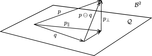
As in Euclidean geometry, we can view
 $p$
as being decomposed into a component
 $p_\|$
lying in
 $\mathcal{Q}$
and a component
 $p_\perp$
perpendicular to it; therefore
 $q^\star = p_\|$
(see Fig. 1).
Projection onto a subspace,
 $\mathcal{Q}$
, of the Bayesian Hilbert space,
 ${\mathcal{B}}^2$
.

The coordinates of
 $q^\star$
can be calculated as
 \begin{equation} \boldsymbol \alpha ^\star = \left \langle{\textbf{b}},{\textbf{b}}\right \rangle ^{-1}\left \langle{\textbf{b}},{p}\right \rangle. \end{equation}
We may also write the projection as an outer product operation on
 $p$
, as detailed in Appendix B.
3.2. Example: one-dimensional Gaussian
To make the concept of Bayes space more tangible, consider the canonical one-dimensional Gaussian PDF defined over
 $x \in \mathbb{R}$
:
 \begin{equation} p(x) = \frac{1}{\sqrt{2 \pi \sigma ^2}} \exp \left ( -\frac{1}{2} \frac{(x-\mu )^2}{\sigma ^2} \right ), \end{equation}
where
 $\mu$
is the mean and
 $\sigma ^2$
the variance. In the language of
 ${\mathcal{B}}^2$
, we can write this as
 \begin{equation} p(x) = \underbrace{\left ( -\frac{\mu }{\sigma ^2}\right )}_{\alpha _1} \cdot \underbrace{\exp (\!-\!x)}_{b_1} \oplus \underbrace{\left (\frac{1}{\sqrt{2}\sigma ^2}\right )}_{\alpha _2} \cdot \underbrace{\exp \left ( -\frac{(x^2 - 1)}{\sqrt{2}} \right )}_{b_2} = \alpha _1 \cdot b_1 \oplus \alpha _2 \cdot b_2. \end{equation}
In other words, every Gaussian can be written as a linear combination of the two vectors,
 $b_1$
and
 $b_2$
, where the coefficients,
 $\alpha _1$
and
 $\alpha _2$
, depend on the mean and variance. Note, we can neglect the normalizing constant as equivalence is implied in the “
 $=$
” operator.
The choice of
 $b_1$
and
 $b_2$
is not arbitrary in this example. They constitute the first two basis vectors in an orthonormal basis for
 ${\mathcal{B}}^2$
, which can be established using the probabilist’s Hermite polynomials; Appendix C.1 provides the details of this Hermite basis. In fact, we can define a new space
 $\mathcal{G}$
as the span of these two basis vectors:
 \begin{equation}{\mathcal{G}} = \text{span}\left \{ b_1, b_2 \right \}, \end{equation}
which is a subspace of
 ${\mathcal{B}}^2$
. Importantly, every Gaussian PDF of the form in (19) is a member of
 $\mathcal{G}$
, but not every member of
 $\mathcal{G}$
is a valid Gaussian PDF. Only those members of
 $\mathcal{G}$
that have
 $\sigma ^2 \gt 0$
are valid Gaussian PDFs. We shall refer to
 $\mathcal{G}$
as the indefinite-Gaussian subspace of
 ${\mathcal{B}}^2$
while
 $\,\downarrow \!{{\mathcal{G}}} \subset{\mathcal{G}}$
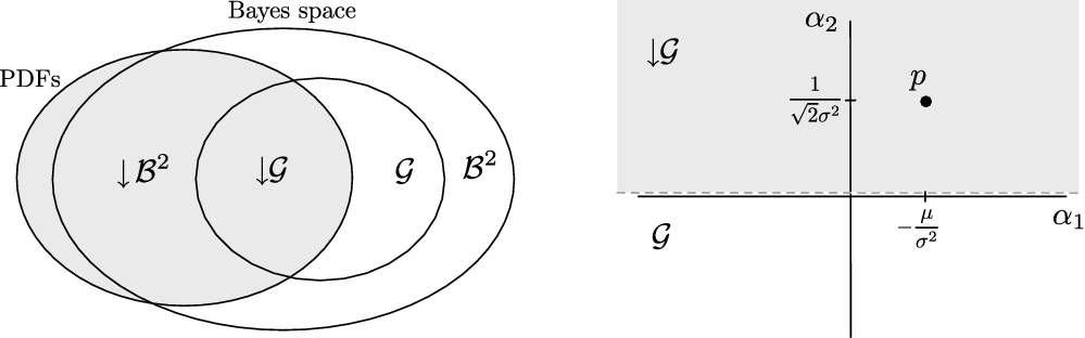
will denote the positive-definite-Gaussian subset. Figure 2 shows the relationships between the various spaces and how we can view a Gaussian as a point in
 $\mathcal{G}$
.
3.3. Example: projecting to a Gaussian
Let us consider a simple one-dimensional, nonlinear estimation problem as a numerical example motivated by the type of inverse-distance nonlinearity found in a stereo camera model. This same experiment (with the same parameter settings) was used as a running example by [[Reference Barfoot10], Section 4]. We assume that our true state is drawn from a Gaussian prior:
 \begin{equation} x \sim \mathcal{N}(\mu _p, \sigma _p^2). \end{equation}
We then generate a measurement according to
 \begin{equation} z = \frac{fb}{x} + n, \quad n \sim \mathcal{N}(0,\sigma _r^2), \end{equation}
where
 $n$
is the measurement noise. The numerical values of the parameters used were
 \begin{equation} \begin{gathered} \mu _p = 20 \text{ [m]}, \quad \sigma _p^2 = 9 \text{ [m$^2$]}, \\[2pt] f = 400 \text{ [pixel]}, \quad b = 0.1 \text{ [m]}, \quad \sigma _r^2 = 0.09 \text{ [pixel$^2$]}. \end{gathered} \end{equation}
On the left is a depiction of the relationships between Bayes space,
 ${\mathcal{B}}^2$
, and the set of all PDFs. We see the subset of strictly positive PDFs,
 $\,\downarrow \!{{\mathcal{B}}^2}$
, the indefinite-Gaussian subspace,
 $\mathcal{G}$
, and the positive-definite-Gaussian subset,
 $\,\downarrow \!{{\mathcal{G}}}$
. The right image shows how a valid Gaussian PDF can be viewed as a point in a plane with coordinates that depend on its mean
 $\mu$
and variance
 $\sigma ^2$
; only the open upper-half plane admits valid Gaussian PDFs since we must have
 $\sigma ^2 \gt 0$
.

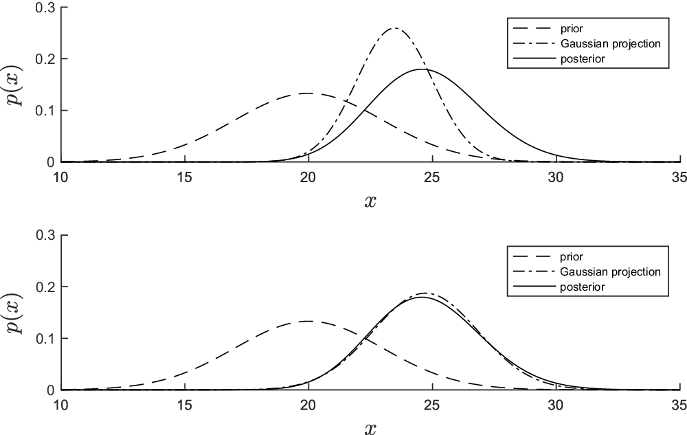
An example of projecting a non-Gaussian posterior onto the indefinite-Gaussian subspace. The top panel shows the case where the measure associated with
 ${\mathcal{B}}^2$
was chosen to be the same as the (Gaussian) prior,
 $\nu (x) = \mathcal{N}(20,9)$
. The bottom panel does the same with a Gaussian measure selected to be closer to the posterior,
 $\nu (x) = \mathcal{N}(24,4)$
. We see that the Gaussian projection of the posterior is much closer to the true posterior in the bottom case.

The true posterior is given by
 \begin{equation} p(x|z) = \,\downarrow \!{\exp (\!-\phi (x))}, \quad \phi (x) = \underbrace{\frac{1}{2} \frac{(x - \mu _p)^2}{\sigma _p^2}}_{\text{prior}} + \underbrace{\frac{1}{2} \frac{\left (z - \frac{fb}{x}\right )^2}{\sigma _r^2}}_{\text{measurement}}. \end{equation}
This problem can also be viewed as the correction step of the Bayes filter [Reference Jazwinski26]: Start from a prior and correct it based on the latest (nonlinear) measurement.
We seek to find
 $q(x) \in \,\downarrow \!{{\mathcal{G}}}$
that is a good approximation to the true posterior
 $p(x|z)$
. To do this, we will simply project the posterior onto the indefinite-Gaussian subspace, using the method described in Section 3.1, and then normalize the result. Figure 3 shows the results of doing this for two cases that differ only in the measure
 $\nu$
that we associate with Bayes space. The expectations used in the projections were computed with generic numerical integration although, as discussed by [Reference Barfoot, Forbes and Yoon14], there are several other options including Gaussian quadrature. In the top case, the measure is chosen as the prior estimate, while in the bottom case it is chosen to be closer to the posterior. In both cases, we see that our projection method produces a valid PDF, but in the bottom case the result is much closer to the true posterior. This simple example provides motivation for the main point of this paper, which is that to use the tools of Bayes space effectively, we will seek to iteratively update the measure used to carry out our projections such that we can best approximate a posterior. Intuitively, this makes sense since the measure is providing a weighting to different parts of
 $\mathbb{R}$
so we would like to choose it to pay close attention where the posterior ends up.
4. Variational Bayesian inference
Motivated by the example in Section 3.3, we shall now address the problem of variational Bayesian inference using the algebraic tools of Bayes space.
4.1. Variation on the KL divergence
In variational Bayesian inference, we seek to find an approximation,
 $q$
, from some family of distributions constituting a subspace
 $\mathcal{Q}$
to the true Bayesian posterior
 $p \in{\mathcal{B}}^2$
. In general,
 \begin{equation}{\mathcal{Q}} \subseteq{\mathcal{B}}^2, \end{equation}
where equality will always ensure that
 $q=p$
will match the posterior exactly. But
 ${\mathcal{B}}^2$
is infinite-dimensional and, in practice,
 ${\mathcal{Q}} \subset{\mathcal{B}}^2$
is a finite-dimensional subspace.
There are many possible divergences that can be defined to characterize the “closeness” of
 $q$
to
 $p$
including the KL divergence [Reference Kullback and Leibler28], Bregman divergence [Reference Bregman19], Wasserstein divergence/Earth mover’s distance [Reference Monge35], and Rényi divergence [Reference Rényi38]. We shall focus on the KL divergence, which is defined as
 \begin{equation} \text{KL}(q || p) = - \int _{\mathcal{X}} q(\textbf{x}) \ln \left ( \frac{p(\textbf{x} | \textbf{z})}{q(\textbf{x})} \right ) \, d\textbf{x} = -\mathbb{E}_q [ \ln p - \ln q]. \end{equation}
Sometimes the reverse of this is used:
 $\text{KL}(p || q)$
. Note, we show the divergence with respect to the posterior,
 $p(\textbf{x} | \textbf{z})$
, but in practice during the calculations we use that
 $p(\textbf{x} | \textbf{z}) = p(\textbf{x},\textbf{z})/ p(\textbf{z}) = \,\downarrow \!{p(\textbf{x},\textbf{z})}$
since the joint likelihood is easy to construct and then the
 $p(\textbf{z})$
can be dropped for it does not result in a KL term that depends on
 $\textbf{x}$
. We will generically use
 $p$
in what follows to keep the notation clean.
4.2. KL gradient
We assume a basis
 $B = \{b_1,b_2\cdots b_M\}$
for
 $\mathcal{Q}$
and we write
 $q$
as
 \begin{equation} q = \,\downarrow \!{} \bigoplus _{m=1}^M \alpha _m\cdot b_m. \end{equation}
We desire to minimize the KL divergence with respect to the coordinates
 $\alpha _m$
. The gradient of
 $\text{KL}(q || p)$
can be computed as follows:
 \begin{equation} \frac{\partial \text{KL}}{\partial \alpha _n} = -\int _{{\mathcal{X}}} \left (\frac{\partial q}{\partial \alpha _n}(\ln p - \ln q) - q\frac{\partial \ln q}{\partial \alpha _n}\right )d\textbf{x}. \end{equation}
Exploiting (E4) and (E6), this reduces to
 \begin{equation} \frac{\partial \text{KL}}{\partial \alpha _n} = -{\mathbb{E}}_q[\ln b_n(\ln p - \ln q)] +{\mathbb{E}}_q[\ln b_n]{\mathbb{E}}_q[\ln p - \ln q] = -\left \langle{b_n},{p\ominus q}\right \rangle _q \end{equation}
or, collecting these in matrix form,
 \begin{equation} \frac{\partial \text{KL}}{\partial \boldsymbol \alpha ^T} = -\left \langle{\textbf{b}},{p\ominus q}\right \rangle _q, \end{equation}
where
 $\textbf{b} = \begin{bmatrix} b_1 & b_2 & \cdots & b_M \end{bmatrix}^T$
. Implicit in this statement is that when employed as the measure, we have normalized the current approximation,
 $\,\downarrow \!{q^{(i)}}$
, since we always take the measure to be a valid PDF. The necessary condition for a minimum of the KL divergence is that the gradient is zero. Newton’s method suggests the manner in which we might iteratively solve for the optimal distribution. Following the established procedure, the iteration for the coordinates is given by
 \begin{equation} \boldsymbol \alpha ^{(i+1)} = \boldsymbol \alpha ^{(i)} +{\textbf{H}^{(i)}}^{-1}\left \langle{\textbf{b}},{p\ominus q^{(i)}}\right \rangle _{q^{(i)}}, \end{equation}
where
 $\textbf{H}$
is the Hessian of the KL divergence.
4.3. KL Hessian
The
 $(m,n)$
entry of the Hessian is
 \begin{equation} \frac{\partial ^2\text{KL}}{\partial \alpha _m\partial \alpha _n} = -\frac{\partial }{\partial \alpha _m}\left \langle{b_n},{p\ominus q}\right \rangle _q. \end{equation}
This differentiation must take into account the effect of the “measure”
 $q$
. The product rule applies here and we can break down the differentiation as
 \begin{equation} \frac{\partial ^2\text{KL}}{\partial \alpha _m\partial \alpha _n} = -\left (\frac{\partial }{\partial \alpha _m}\left \langle{b_n},{p\ominus q}\right \rangle \right )_q - \left \langle{b_n},{p\ominus q}\right \rangle _{\partial q/\partial \alpha _m}, \end{equation}
the first term of which is to be read as the derivative of the inner product holding the measure fixed and the second of which deals with the derivative of the measure while holding the arguments of inner product fixed. The first term is
 \begin{equation} \left (\frac{\partial }{\partial \alpha _m}\left \langle{b_n},{p\ominus q}\right \rangle \right )_q = \left (\frac{\partial }{\partial \alpha _m}\left \langle{b_n},{p}\right \rangle - \frac{\partial }{\partial \alpha _m}\sum _k\alpha _k\left \langle{b_n},{b_k}\right \rangle \right )_q = -\left \langle{b_n},{b_m}\right \rangle _q = -\left \langle{b_m},{b_n}\right \rangle _q. \end{equation}
As shown in Appendix E.2, the second becomes
 \begin{equation} \left \langle{b_n},{p\ominus q}\right \rangle _{\partial q/\partial \alpha _m} = \left \langle{b_n},{\frac{\partial \ln q}{\partial \alpha _m}\cdot (p\ominus q)}\right \rangle _q -{\mathbb{E}}_q[\ln p - \ln q]\left \langle{b_m},{b_n}\right \rangle _q. \end{equation}
We advise that the coefficient
 $\partial \ln q/\partial \alpha _m$
of
 $p\ominus q$
is in fact a function of the state and as such cannot be transferred to the other argument of the inner product as would be possible for a scalar in the field
 $\mathbb{R}$
. We also recognize the factor of the last term as
 $\text{KL}(q||p)$
. Therefore, substituting (35) and (36) into (34) yields
 \begin{equation} \frac{\partial ^2\text{KL}}{\partial \alpha _m\partial \alpha _n} = \left (1 - \text{KL}(q||p)\right )\left \langle{b_m},{b_n}\right \rangle _q - \left \langle{b_n},{\frac{\partial \ln q}{\partial \alpha _m}\cdot (p\ominus q)}\right \rangle _q. \end{equation}
We observe that the second term on the right-hand side is symmetric in the indices as the substitution of (E6) will attest. In matrix form, the Hessian is
 \begin{equation} \textbf{H} = \frac{\partial ^2\text{KL}}{\partial \boldsymbol \alpha ^T\partial \boldsymbol \alpha } = \left (1 - \text{KL}(q||p)\right )\textbf{I}_{\boldsymbol \alpha } - \left \langle{\textbf{b}},{\frac{\partial \ln q}{\partial \boldsymbol \alpha ^T}\cdot (p\ominus q)}\right \rangle _q, \end{equation}
where
 $\textbf{I}_{\boldsymbol \alpha }$
is the Fisher information matrix (FIM) or Gram matrix and is described in detail in Appendix E.1. Newton’s method (32) can now be implemented. But the Hessian bears a closer look.
The Hessian can also be explicitly written as
 \begin{align} \frac{\partial ^2\text{KL}}{\partial \alpha _m\partial \alpha _n} &= \left \langle{b_m},{b_n}\right \rangle _q -{\mathbb{E}}_q[\ln b_m\ln b_n(\ln p - \ln q)] \nonumber \\[5pt] &+{\mathbb{E}}_q[\ln b_m\ln b_n]{\mathbb{E}}_q[\ln p - \ln q] +{\mathbb{E}}_q[\ln b_n]{\mathbb{E}}_q[\ln b_m(\ln p - \ln q)] \nonumber \\[5pt] &+{\mathbb{E}}_q[\ln b_m]{\mathbb{E}}_q[\ln b_n(\ln p - \ln q)] - 2{\mathbb{E}}_q[\ln b_m]{\mathbb{E}}_q[\ln b_n]{\mathbb{E}}_q[\ln p - \ln q], \end{align}
the terms of which can be collected as
 \begin{equation} \frac{\partial ^2\text{KL}}{\partial \alpha _m\partial \alpha _n} = \left \langle{b_m},{b_n}\right \rangle _q + \left \langle{-b_{mn} \oplus {\mathbb{E}}_q[\ln b_n]\cdot b_m \oplus{\mathbb{E}}_q[\ln b_m]\cdot b_n},{p\ominus q}\right \rangle _q, \end{equation}
where
 $b_{mn} = \exp (\ln b_m\ln b_n)$
. The symmetry in the Hessian is plainly evident in this version.
4.4. Iterative projection
In the vicinity of the optimal distribution, with a sufficiently large subspace
 $\mathcal{Q}$
, we may expect
 $p\ominus q$
to be small almost everywhere. This makes all the terms in the Hessian of first order except
 $\textbf{I}_{\boldsymbol \alpha }$
, which is of zeroth order. The gradient (68) is also of first order. Thus to keep Newton’s descent to this order, we may approximate the Hessian as
 $\textbf{H} \simeq \textbf{I}_{\boldsymbol \alpha }$
and the iterative procedure (32) becomes simply
 \begin{equation} \boldsymbol \alpha ^{(i+1)} = \boldsymbol \alpha ^{(i)} +{\textbf{I}_{\boldsymbol \alpha }^{(i)}}^{-1}\left \langle{\textbf{b}},{p\ominus q^{(i)}}\right \rangle _{q^{(i)}}. \end{equation}
However, as
 $q^{(i)} = \,\downarrow \!{\bigoplus }_m \alpha _m^{(i)}\cdot b_m$
,
 \begin{equation} \left \langle{\textbf{b}},{p\ominus q^{(i)}}\right \rangle _{q^{(i)}} = \left \langle{\textbf{b}},{p}\right \rangle _{q^{(i)}} - \left \langle{\textbf{b}},{\textbf{b}}\right \rangle _{q^{(i)}}\boldsymbol \alpha ^{(i)} = \left \langle{\textbf{b}},{p}\right \rangle _{q^{(i)}} - \textbf{I}_{\boldsymbol \alpha }^{(i)}\boldsymbol \alpha ^{(i)}. \end{equation}
Hence, (41) becomes
 \begin{equation} \boldsymbol \alpha ^{(i+1)} ={\textbf{I}_{\boldsymbol \alpha }^{(i)}}^{-1}\left \langle{\textbf{b}},{p}\right \rangle _{q^{(i)}}. \end{equation}
The iterative update to
 $q$
is
 $q^{(i+1)} = \,\downarrow \!{\bigoplus }_m \alpha _m^{(i+1)}\cdot b_m$
. That is, the procedure can be viewed as an iterative projection,
 \begin{equation} q^{(i+1)} = \underset{({\mathcal{Q}}, q^{(i)})}{\,\downarrow \!{} \text{proj}} p, \end{equation}
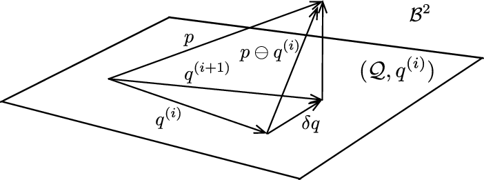
where we explicitly indicate that we normalize the result as the output of our algorithm should be a PDF. Figure 4 depicts the scheme. The procedure is essentially the application of Newton’s method on the KL divergence with the Hessian approximated as the FIM. This is precisely the approximation made in natural gradient descent [Reference Amari4]. In our Bayesian space, the operating point of the Newton step becomes the measure for the inner product. This highlights a key aspect of using the algebra associated with a Bayesian space. It recognizes the dual role of
 $q$
: On the one hand, it is the approximating PDF, and on the other it serves as a measure that weights the difference between the approximation and the approximated.
Iterative projection onto a sequence of Bayesian Hilbert spaces,
 $(\mathcal{Q},q^{(i)})$
.

Convergence of iterative projection is guaranteed if the Hessian is positive definite. Provided that the subspace is large enough, we can expect convergence when we begin in a neighborhood of optimal
 $q$
where the first-order terms in the Hessian are sufficiently small.
It is notable that each step of the iterative projection is equivalent to the local minimization of the divergence
 $I(p\ominus q)$
with the measure fixed at
 $q^{(i)}$
because
 \begin{equation} I\!\left (p\ominus ( q^{(i)}\oplus \delta q)\right ) = I(p\ominus q^{(i)}) + \delta \boldsymbol \alpha ^T\left (\frac{\partial I}{\partial \boldsymbol \alpha ^T}\right )_{q^{(i)}} + \frac{1}{2}\delta \boldsymbol \alpha ^T \left (\frac{\partial ^2 I}{\partial \boldsymbol \alpha ^T\partial \boldsymbol \alpha }\right )_{q^{(i)}} \delta \boldsymbol \alpha, \end{equation}
where
 $\delta \boldsymbol \alpha = \boldsymbol \alpha ^{(i+1)} - \boldsymbol \alpha ^{(i)}$
and
 \begin{equation} \left (\frac{\partial I}{\partial \boldsymbol \alpha ^T}\right )_{q^{(i)}} = -\left \langle{\textbf{b}},{p\ominus q^{(i)}}\right \rangle _{q^{(i)}}, \quad \left (\frac{\partial ^2 I}{\partial \boldsymbol \alpha ^T\partial \boldsymbol \alpha }\right )_{q^{(i)}} = \left \langle{\textbf{b}},{\textbf{b}}\right \rangle _{q^{(i)}} \equiv \textbf{I}_{\boldsymbol \alpha }^{(i)}, \end{equation}
which are identical to the linearized forms for the KL divergence.
Throughout this section, we have assumed that the basis
 $B$
remains constant across iterations, but this need not be the case. We may also choose to update the basis along with the measure to maintain, for example, orthonormality. This is explored in the next example and further in Section 5 on Gaussian variational inference.
4.5. Example: iteratively projecting to a Gaussian
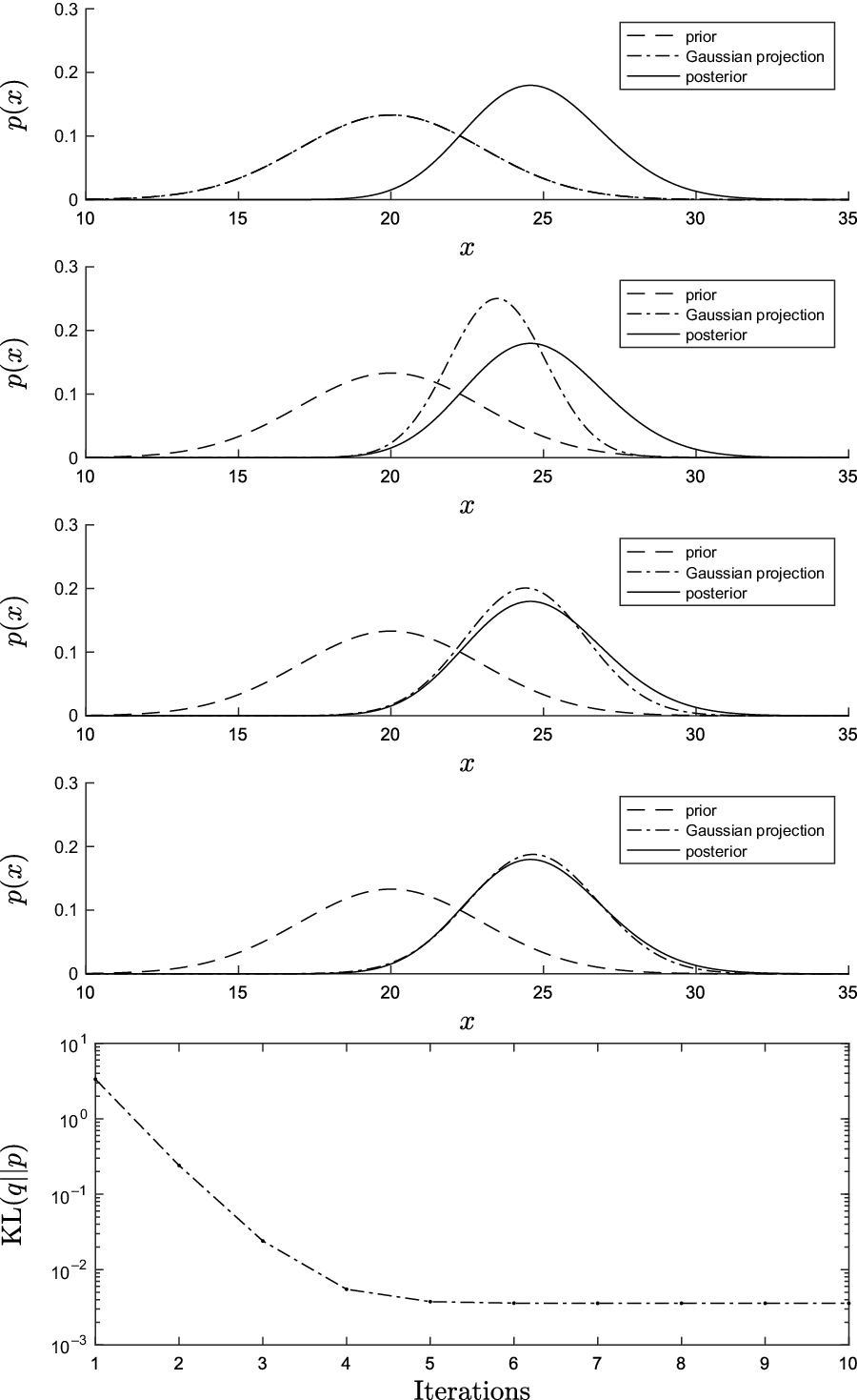
In the example of Section 3.3, we saw that selecting a measure that was closer to the posterior resulted in a projection that was also closer to the posterior. We now redo this example using the iterative projection concepts from this section. We will still project onto the indefinite-Gaussian subspace and employ a Gaussian measure, only now with each iteration the measure will be taken to be the (normalized) projection from the previous iteration.
We initialized the estimate to the prior, which corresponds to the first panel in Fig. 5. The next three panels show subsequent iterations of the estimate. The last panel shows the KL divergence between the estimate and the true posterior for 10 iterations. We see the estimate converged in a few iterations.
Example of iterative projection onto the indefinite-Gaussian subspace spanned by two Hermite basis functions, where the measure is taken to be the estimate
 $q^{(i)}$
at the previous iteration and the basis reorthogonalized at each iteration as described in Section 5. The estimate was initialized to the prior (first panel) and then iteratively updated (next three panels). The last panel shows the KL divergence between the estimate and the true posterior for 10 iterations, with convergence occurring at approximately 5 iterations.

Note that as the measure changes from one iteration to the next, we then have to update the basis to retain the desired orthogonality. This can be accomplished by using the reparameterization “trick” (see Appendix C.1) to adjust the basis to be orthogonal with respect to the current Gaussian measure.
4.6. Exploiting sparsity
One of the major advantages of thinking of
 ${\mathcal{B}}^2$
as a vector space with the definition of vector addition
 $\oplus$
is that Bayesian inference in general can be viewed as the addition of vectors. Consider the posterior
 $p(\textbf{x} | \textbf{z})$
where
 $\textbf{z}$
are some measurements. Bayes’ rule states that
 \begin{equation} p(\textbf{x} | \textbf{z}) = \frac{p(\textbf{z} | \textbf{x}) p(\textbf{x})}{p(\textbf{z})} = p(\textbf{z} | \textbf{x}) \oplus p(\textbf{x}), \end{equation}
where
 $p(\textbf{x})$
is a prior,
 $p(\textbf{z} | \textbf{x})$
is a measurement factor and, as mentioned earlier, we need not introduce the normalization constant
 $p(\textbf{z})$
explicitly when writing the posterior as a vector addition in Bayesian space. To be clear, addition is defined for two members of the same Bayes space and here we interpret
 $p(\textbf{z} | \textbf{x})$
as a function of
 $\textbf{x}$
since
 $\textbf{z}$
is a constant (e.g., a known measurement).
If we have several measurements that are statistically independent, then this can be factored as
 \begin{equation} p(\textbf{x} | \textbf{z}) = p(\textbf{x}) \oplus \bigoplus _{k=1}^K p(\textbf{z}_k | \textbf{x}_k), \end{equation}
where
 $\textbf{x}_k = \textbf{P}_k \textbf{x}$
is a subset of the variables in
 $\textbf{x}$
,
 $\textbf{P}_k$
is a projection matrix, and
 $\textbf{z}_k$
is the
 $k$
th measurement. This expresses sparsity in the state description and in the measurements. To keep the notation economical, we shall simply write
 \begin{equation} p = \bigoplus _{k=0}^K p_k, \end{equation}
where
 $p$
is the posterior and the
 $p_k$
comprise the prior and the measurements, corresponding to statistically independent data. In other words, the factorization becomes a summation in the Bayesian space
 ${\mathcal{B}}^2$
.
Now consider our projective approach to inference. As usual, given a subspace
 ${\mathcal{Q}} \subset{\mathcal{B}}^2$
, the optimal estimate to (49) is given by
 \begin{equation} q^\star = \underset{{\mathcal{Q}}}{\text{proj}} \, p = \underset{{\mathcal{Q}}}{\text{proj}} \,\bigoplus _{k=0}^K p_k = \bigoplus _{k=0}^K \underset{{\mathcal{Q}}}{\text{proj}} \, p_k. \end{equation}
That is, the projection of the sum is the sum of the projections. Each individual projection can be done separately because we are in a linear space. This is of enormous practical advantage because it means that we do not need all of
 $\mathcal{Q}$
to represent each projection.
We can see this more clearly by defining
 ${\mathcal{B}}^2_k \subset{\mathcal{B}}^2$
as the subspace corresponding to the variables
 $\textbf{x}_k$
. Then
 \begin{equation} p = \bigoplus _{k=0}^K p_k \in{\mathcal{B}}^2_0\oplus{\mathcal{B}}^2_1\oplus \cdots \oplus{\mathcal{B}}^2_K \subseteq{\mathcal{B}}^2. \end{equation}
In other words,
 $p$
is contained in the direct sum of the subspaces
 ${\mathcal{B}}^2_k$
. Each constituent part
 $p_k$
may be confined to a smaller subspace of
 ${\mathcal{B}}^2$
, depending on the variable dependencies in each term.
If we wish to project
 $p_k \in{\mathcal{B}}^2_k$
onto
 $\mathcal{Q}$
it will suffice to consider the projection on just
 ${\mathcal{Q}}_k ={\mathcal{B}}^2_k \cap{\mathcal{Q}}$
, that is,
 \begin{equation} \underset{{\mathcal{Q}}}{\text{proj}} \, p_k = \underset{{\mathcal{Q}}_k}{\text{proj}} \, p_k. \end{equation}
The subspace
 ${\mathcal{Q}}_k$
may, and ideally would, be smaller than
 $\mathcal{Q}$
. We may refer to
 ${\mathcal{Q}}_k$
as the marginal subspace of
 $\mathcal{Q}$
with respect to the subset of variables
 $\textbf{x}_k$
.
Therefore, the optimal estimate will be given by
 \begin{equation} q^\star = \underset{{\mathcal{Q}}}{\text{proj}} \, p = \bigoplus _{k=0}^K \underset{{\mathcal{Q}}_k}{\text{proj}} \, p_k. \end{equation}
Exploiting sparsity by projecting individual measurements onto marginal subspaces,
 $\mathcal{Q}_k$
, and then recombining the results.

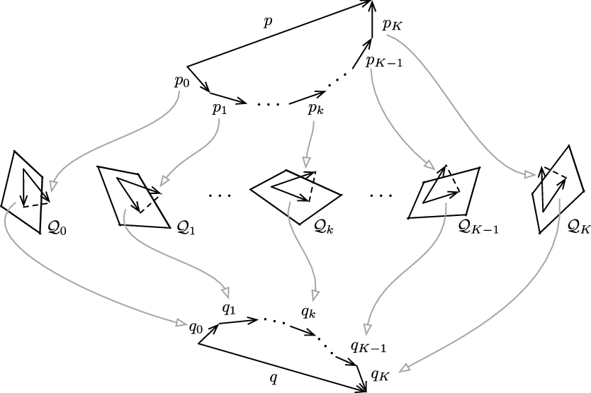
This means that we can project the PDF associated with each measurement onto a smaller subspace and simply add up the estimates, lifting the overall estimate up into a potentially much larger space. Naturally, when employed in practice we will normalize
 $q^\star$
to ensure our algorithm outputs a valid PDF. The decomposition and reconstitution are illustrated in Fig. 6. Just as with the total posterior, we may describe
 $q^\star$
as being an element of a direct sum of the individual subspaces of
 $\mathcal{Q}$
, that is,
 \begin{equation} q^\star \in{\mathcal{Q}}_0 \oplus{\mathcal{Q}}_1 \oplus \cdots \oplus{\mathcal{Q}}_K \subseteq{\mathcal{Q}}. \end{equation}
The subspace sum may be substantially smaller than
 $\mathcal{Q}$
but again it will depend on the variable dependencies of each term.
This is the key result that allows most practical inference frameworks to function in a tractable way. Depending on the chosen basis for
 $\mathcal{Q}$
, many of the coordinates can potentially be zero and thus it will not be necessary to waste effort computing them or space storing them.
5. Application: Iterative projection for multivariate Gaussians
Let us investigate a little more closely iterative projection to multivariate Gaussian PDFs, given their importance in statistics and estimation theory.
5.1. Projections
As mentioned at the end of the last section, we do not have to maintain the same basis from step to step as long as each basis spans the same subspace. This is a particularly useful maneuver when using the subspace
 $\mathcal{G}$
of indefinite Gaussians, which are discussed in detail for the multivariate case in Appendix D.1. Denote the mean and variance of
 $q^{(i)} \in{\mathcal{G}}$
as
 ${\boldsymbol{\mu }}^{(i)}$
and
 $\boldsymbol{\Sigma }^{(i)}$
and let the basis
 $\textbf{g}^{(i)}$
be defined as in (D3) and (D4). Note that this basis is orthonormal with respect to
 $q^{(i)}$
. As such,
 $\textbf{I}_{\boldsymbol \alpha }^{(i)} = \langle{\textbf{g}^{(i)}},{\textbf{g}^{(i)}} \rangle _{q^{(i)}} = \textbf{1}$
. Imagine the PDF to be approximated is expressed as
 $p = \,\downarrow \!{\exp (\!-\phi (\textbf{x}))} \in \,\downarrow \!{{\mathcal{B}}^2}$
. The coordinates resulting from the next projection are given by (D13), namely,
 \begin{equation} \begin{gathered} \boldsymbol \alpha _1^{(i+1)} = \left \langle{\textbf{g}_1^{(i)}},{p}\right \rangle ={\textbf{L}^{(i)}}^T{\mathbb{E}}_{q^{(i)}}\left [\frac{\partial \phi (\textbf{x})}{\partial \textbf{x}^T}\right ], \\[10pt] \boldsymbol \alpha _2^{(i+1)} = \left \langle{\textbf{g}_2^{(i)}},{p}\right \rangle = \sqrt{\text{$\frac{1}{2}$}\textbf{D}^T\textbf{D}}\, \text{vech}\left ({\textbf{L}^{(i)}}^T{\mathbb{E}}_{q^{(i)}}\left [\frac{\partial ^2\phi (\textbf{x})}{\partial \textbf{x}^T\partial \textbf{x}}\right ]{\textbf{L}^{(i)}}\right ), \end{gathered} \end{equation}
where
 $\textbf{L}^{(i)}$
issues from the Cholesky decomposition of
 $\boldsymbol{\Sigma }^{(i)}$
.
The new iteration is
 \begin{equation} q^{(i+1)} = \underset{({\mathcal{G}}, q^{(i)})}{\,\downarrow \!{}\text{proj}} \,p = \,\downarrow \!{\exp }\left (\!-{\boldsymbol \alpha _1^{(i+1)}}^T{\boldsymbol{\gamma }}_1^{(i)} -{\boldsymbol \alpha _1^{(i+1)}}^T{\boldsymbol{\gamma }}_1^{(i)}\right ). \end{equation}
Using (D14), this becomes
 \begin{equation} q^{(i+1)} = \,\downarrow \!{\exp }\biggl (\!-(\textbf{x} -{\boldsymbol{\mu }}^{(i)})^T{\mathbb{E}}_{q^{(i)}}\left [\frac{\partial \phi (\textbf{x})}{\partial \textbf{x}^T}\right ] -\frac{1}{2}(\textbf{x} -{\boldsymbol{\mu }}^{(i)})^T{\mathbb{E}}_{q^{(i)}}\left [\frac{\partial ^2\phi (\textbf{x})}{\partial \textbf{x}^T\partial \textbf{x}}\right ] (\textbf{x} -{\boldsymbol{\mu }}^{(i)})\biggr ), \end{equation}
which we may cast into the form,
 \begin{equation} q^{(i+1)} = \,\downarrow \!{\exp }\!\left (\!-\frac{1}{2}(\textbf{x} -{\boldsymbol{\mu }}^{(i+1)})^T{\boldsymbol{\Sigma }^{(i+1)}}^{-1} (\textbf{x} -{\boldsymbol{\mu }}^{(i+1)})\right ). \end{equation}
Herein
 \begin{equation} {\boldsymbol{\Sigma }^{(i+1)}}^{-1} ={\mathbb{E}}_{q^{(i)}}\left [\frac{\partial ^2\phi (\textbf{x})}{\partial \textbf{x}^T\partial \textbf{x}}\right ], \end{equation}
 \begin{equation} {\boldsymbol{\Sigma }^{(i+1)}}^{-1}\delta{\boldsymbol{\mu }} = -{\mathbb{E}}_{q^{(i)}}\left [\frac{\partial \phi (\textbf{x})}{\partial \textbf{x}^T}\right ], \end{equation}
 \begin{equation} {\boldsymbol{\mu }}^{(i+1)} ={\boldsymbol{\mu }}^{(i)} + \delta{\boldsymbol{\mu }} \end{equation}
give the updates from
 $q^{(i)} ={\mathcal{N}}({\boldsymbol{\mu }}^{(i)},\boldsymbol{\Sigma }^{(i)})$
to
 $q^{(i+1)} ={\mathcal{N}}({\boldsymbol{\mu }}^{(i+1)},\boldsymbol{\Sigma }^{(i+1)})$
and these are exactly the same as those used in the iterative Gaussian variational inference approach presented by [Reference Barfoot, Forbes and Yoon14]. We have arrived at the same variational updates but have done so from the framework of a Bayesian Hilbert space, where it becomes abundantly clear that the minimization algorithm is in fact a slightly simplified version of Newton’s method. This also provides the connection back to the classic Gaussian filtering and smoothing algorithms as discussed by [Reference Barfoot, Forbes and Yoon14].
5.2. Sparsity in Gaussian inference
The effect of sparsity as it applies to iterative Gaussian inference is of particular interest. Let us consider the decomposition of a posterior
 $p$
in accordance to the general sparsity discussion in Section 4.6, that is,
 \begin{equation} p = \,\downarrow \!{\exp (\!-\phi (\textbf{x}))} = \,\downarrow \!{\exp \left (\!-\sum _{k=0}^K \phi _k( \textbf{x}_k )\right )} = \,\downarrow \!{\bigoplus_{k=0}^K} \exp \left (\!-\phi _k( \textbf{x}_k )\right ) = \,\downarrow \!{\bigoplus_{k=0}^K} p_k, \end{equation}
where
 $\phi _k(\textbf{x}_k)$
is the
 $k$
th (negative log) factor expression and
 $\textbf{x}_k = \textbf{P}_k\textbf{x}$
.
As in (D14), we may express the variational estimate as
 \begin{align} q^{(i+1)} = \underset{({\mathcal{G}},q^{(i)})}{\,\downarrow \!{}\text{proj}} \, p = \,\downarrow \!{\exp }\biggl ( -(\textbf{x} -{\boldsymbol{\mu }}^{(i)})^T\mathbb{E}_{q^{(i)}} \left [ \frac{\partial \phi (\textbf{x})}{\partial \textbf{x}^T}\right ]- \frac{1}{2} (\textbf{x} -{\boldsymbol{\mu }}^{(i)})^T \, \mathbb{E}_{q^{(i)}} \left [ \frac{\partial ^2 \phi (\textbf{x})}{\partial \textbf{x}^T \partial \textbf{x}} \right ] (\textbf{x} -{\boldsymbol{\mu }}^{(i)})\biggr ), \end{align}
using the measure
 $q^{(i)} = \mathcal{N}({\boldsymbol{\mu }}^{(i)}, \boldsymbol{\Sigma }^{(i)})$
. To take advantage of sparsity, we need to have it reflected in the expectations herein. The first one leads to
 \begin{align} {\mathbb{E}}_{q^{(i)}}\left [\frac{\partial \phi (\textbf{x})}{\partial \textbf{x}^T}\right ] &= \sum _{k=0}^K{\mathbb{E}}_{q^{(i)}}\left [\frac{\partial \phi _k(\textbf{x}_k)}{\partial \textbf{x}^T}\right ] = \sum _{k=0}^K \left (\frac{\partial \textbf{x}_k}{\partial \textbf{x}}\right )^T{\mathbb{E}}_{q^{(i)}}\left [\frac{\partial \phi _k(\textbf{x}_k)}{\partial \textbf{x}_k^T}\right ]\nonumber \\[5pt] &= \sum _{k=0}^K \textbf{P}_k^T{\mathbb{E}}_{q^{(i)}}\left [\frac{\partial \phi _k(\textbf{x}_k)}{\partial \textbf{x}_k^T}\right ] = \sum _{k=0}^K \textbf{P}_k^T{\mathbb{E}}_{q^{(i)}_k}\left [\frac{\partial \phi _k(\textbf{x}_k)}{\partial \textbf{x}_k^T}\right ], \end{align}
given that
 $\textbf{x}_k = \textbf{P}_k\textbf{x}$
. For each factor
 $k$
, then, we are able to shift the differentiation from
 $\textbf{x}$
to
 $\textbf{x}_k$
. We draw attention to the last equality, where the expectation simplifies to using
 $q^{(i)}_k = q^{(i)}_k(\textbf{x}_k)$
, the marginal of the measure for just the variables in factor
 $k$
. In a similar fashion,
 \begin{equation} \mathbb{E}_{q^{(i)}}\left [ \frac{\partial ^2 \phi (\textbf{x})}{\partial \textbf{x}^T \partial \textbf{x}} \right ] = \sum _{k=0}^K \textbf{P}_k^T \,\mathbb{E}_{q_k^{(i)}} \left [ \frac{\partial ^2 \phi _k( \textbf{x}_k )}{\partial \textbf{x}_k^T \partial \textbf{x}_k} \right ] \textbf{P}_k \end{equation}
accounts for the second expectation in (61).
The implication of the factorization is that each factor, identified by
 $\phi _k(\textbf{x}_k)$
, is projected onto
 ${\mathcal{G}}_k$
, the marginal subspace associated with variables
 $\textbf{x}_k$
. The results can then be recombined for the full variational estimate as
 \begin{equation} q^{(i+1)} = \underset{({\mathcal{G}},q^{(i)})}{\,\downarrow \!{}\text{proj}} \, p = \,\downarrow \!{}\bigoplus _{k=0}^K \underset{({\mathcal{G}}_k,q_k^{(i)})}{\text{proj}} \, p_k = \,\downarrow \!{} \bigoplus _{k=0}^K q_k^{(i+1)}. \end{equation}
The individual projections of
 $p_k = \,\downarrow \!{\exp (\!-\phi _k(\textbf{x}_k) )}$
onto
 $({\mathcal{G}}_k,q^{(i)})$
are
 \begin{align} q^{(i+1)}_k & = \underset{({\mathcal{G}}_k,q_k^{(i)})}{\,\downarrow \!{}\text{proj}} \, p_k = \,\downarrow \!{\exp }\left ( -\frac{1}{2} (\textbf{x}_k -{\boldsymbol{\mu }}_k^{(i+1)} )^T \boldsymbol{\Sigma }_k^{(i+1)^{-1}} (\textbf{x}_k -{\boldsymbol{\mu }}_k^{(i+1)} ) \right ) \\[5pt] & = \,\downarrow \!{\exp }\left ( -\frac{1}{2} (\textbf{x} - \textbf{P}_k^T{\boldsymbol{\mu }}_k^{(i+1)} )^T \left ( \textbf{P}_k^T \boldsymbol{\Sigma }_k^{(i+1)^{-1}} \textbf{P}_k \right )(\textbf{x} - \textbf{P}_k^T{\boldsymbol{\mu }}_k^{(i+1)} ) \right ), \end{align}
where
 \begin{equation}{\boldsymbol{\mu }}_k^{(i+1)} ={\boldsymbol{\mu }}_k^{(i)} - \boldsymbol{\Sigma }_k^{(i+1)}{\mathbb{E}}_{q_k^{(i)}}\left [\frac{\partial \phi _k(\textbf{x}_k)}{\partial \textbf{x}_k^T}\right ], \quad \boldsymbol{\Sigma }_k^{(i+1)^{-1}} ={\mathbb{E}}_{q_k^{(i)}}\left [\frac{\partial ^2 \phi _k( \textbf{x}_k )}{\partial \textbf{x}_k^T \partial \textbf{x}_k}\right ]. \end{equation}
It is straightforward to show that the vector sum of
 $q_k$
from (65) reproduces (61). (Note that
 $\textbf{P}_k\textbf{P}_k^T = \textbf{1}$
as
 $\textbf{P}_k$
is a projection matrix and
 $\textbf{P}_k^T$
the corresponding dilation.)
As explained in detail by [Reference Barfoot, Forbes and Yoon14], it would be too expensive for practical problems to construct first
 $\boldsymbol{\Sigma }^{(i)}$
and then extract the required blocks for the marginals,
 $q_k^{(i)} = \mathcal{N}({\boldsymbol{\mu }}_k^{(i)}, \boldsymbol{\Sigma }_k^{(i)}) = \mathcal{N}(\textbf{P}_k{\boldsymbol{\mu }}^{(i)}, \textbf{P}_k\boldsymbol{\Sigma }^{(i)}\textbf{P}_k^T)$
. We see from the above development that we actually only require the blocks of
 $\boldsymbol{\Sigma }^{(i)}$
corresponding to the nonzero blocks of its inverse and the method of [Reference Takahashi, Fagan and Chen41] can be used to extract the required blocks efficiently. In Ref. [Reference Barfoot, Forbes and Yoon14], the authors provide numerical experiments showing the efficacy of this approach.
5.3. Example: SLAM
A main purpose in the current paper was to show the connection between Bayes space [Reference van den Boogaart, Egozcue and Pawlowsky-Glahn43] and Gaussian variational inference [Reference Barfoot, Forbes and Yoon14]. We see that minimizing the KL divergence between a true Bayesian posterior and an approximation can be viewed as iterative projection in Bayes space. Moreover, by exploiting the sparsity that Bayes space makes clear, the method has the potential to be applied to quite large inference problems.
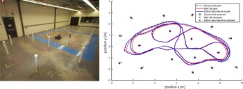
Following [Reference Barfoot, Forbes and Yoon14], we consider a batch SLAM problem with a robot driving around and building a map of landmarks as depicted in Fig. 7. The robot is equipped with a laser rangefinder and wheel odometers and must estimate its own trajectory and the locations of a number of tubular landmarks. This dataset has been used previously by [Reference Barfoot, Tong and Sarkka15] to test SLAM algorithms. Groundtruth for both the robot trajectory and landmark positions (this is a unique aspect of this dataset) is provided by a Vicon motion capture system. The whole dataset is 12,000 timesteps long (approximately 20 min of real time). It was assumed that the data association (i.e., which measurement corresponds to which landmark) is known in this experiment to restrict testing to the state estimation part of the problem.
A special case of the approach presented in this paper was previously demonstrated [Reference Barfoot, Forbes and Yoon14] to be a useful and practical tool for robotic state estimation. The method, called exactly sparse Gaussian variational inference (ESGVI), was used to solve the simultaneous localization and mapping (SLAM) problem, outperforming the standard maximum a posteriori (MAP) estimation in certain cases. The current paper reinterprets this earlier work in a new mathematical formalism. Figure reproduced from [Reference Barfoot, Forbes and Yoon14].

The state to be estimated is
 \begin{equation} \textbf{x} = \begin{bmatrix} \textbf{x}_0 \\[5pt] \textbf{x}_1 \\[5pt] \vdots \\[5pt] \textbf{x}_K \\[5pt] \textbf{m}_1 \\[5pt] \vdots \\[5pt] \textbf{m}_L \end{bmatrix}, \quad \textbf{x}_k = \begin{bmatrix} x_k \\[5pt] y_k \\[5pt] \theta _k \\[5pt] \dot{x}_k \\[5pt] \dot{y}_k \\[5pt] \dot{\theta }_k \end{bmatrix}, \quad \textbf{m}_\ell = \begin{bmatrix} x_\ell \\[5pt] y_\ell \end{bmatrix}, \end{equation}
where
 $\textbf{x}_k$
is a robot state (position, orientation, velocity, angular velocity) and
 $\textbf{m}_\ell$
a landmark position.
For the (linear) prior factor on the robot states, we have
 \begin{equation} \varphi _k = \left \{ \begin{array}{ll} \dfrac{1}{2} (\textbf{x}_0 - \check{\textbf{x}}_0)^T \check{\textbf{P}}^{-1} (\textbf{x}_0 - \check{\textbf{x}}_0) & \quad k=0 \\[12pt] \dfrac{1}{2} (\textbf{x}_k - \textbf{A} \textbf{x}_{k-1})^T \textbf{Q}^{-1} (\textbf{x}_k - \textbf{A} \textbf{x}_{k-1}) \;\;& \quad k\gt 0 \end{array} \right ., \end{equation}
with
 \begin{align} \check{\textbf{P}} = \text{diag}(\sigma _x^2, \sigma _y^2,\sigma _\theta ^2, \sigma _{\dot{x}}^2, \sigma _{\dot{y}}^2, \sigma _{\dot{\theta }}^2), \;\; \textbf{A} = \begin{bmatrix} \textbf{1}\;\;\;\; & T \textbf{1} \\[12pt] \textbf{0}\;\;\;\; & \textbf{1} \end{bmatrix}, \nonumber \\[12pt] \textbf{Q} = \begin{bmatrix} \dfrac{1}{3} T^3 \textbf{Q}_C\;\;\;\; & \dfrac{1}{2} T^2 \textbf{Q}_C \\[12pt] \dfrac{1}{2} T^2 \textbf{Q}_C\;\;\;\; & T \textbf{Q}_C \end{bmatrix}, \quad \textbf{Q}_C = \text{diag}(Q_{C,1}, Q_{C,2},Q_{C,3}), \end{align}
where
 $T$
is the discrete-time sampling period,
 $Q_{C,i}$
are power spectral densities, and
 $\sigma _x^2$
,
 $\sigma _y^2$
,
 $\sigma _\theta ^2$
,
 $\sigma _{\dot{x}}^2$
,
 $\sigma _{\dot{y}}^2$
,
 $\sigma _{\dot{\theta }}^2$
are variances. The robot state prior encourages constant velocity [[Reference Barfoot10], §3, p.85].
The (nonlinear) odometry factors, derived from wheel encoder measurements, are
 \begin{equation} \psi _k = \frac{1}{2} \left ( \textbf{v}_k - \textbf{C}_k \textbf{x}_k \right )^T \textbf{S}^{-1} \left ( \textbf{v}_k - \textbf{C}_k \textbf{x}_k \right ), \end{equation}
where
 \begin{gather} \textbf{v}_k = \begin{bmatrix} u_k \\[5pt] v_k \\[5pt] \omega _k \end{bmatrix}, \quad \textbf{C}_k = \begin{bmatrix} 0\;\;\;\;\; & 0\;\;\;\;\; & 0\;\;\;\;\; & \cos \theta _k \;\;\;\;\; & \sin \theta _k \;\;\;\;\; & 0 \\[5pt] 0\;\;\;\;\; & 0\;\;\;\;\; & 0\;\;\;\;\; & -\sin \theta _k \;\;\;\;\; & \cos \theta _k \;\;\;\;\; & 0 \\[5pt] 0 \;\;\;\;\; & 0 \;\;\;\;\; & 0 \;\;\;\;\; & 0 \;\;\;\;\; & 0 \;\;\;\;\; & 1 \end{bmatrix}, \quad \textbf{S} = \text{diag}\left (\sigma ^2_u, \sigma _v^2, \sigma _\omega ^2 \right ). \end{gather}
The
 $\textbf{v}_k$
consists of measured forward, lateral, and rotational speeds in the robot frame, derived from wheel encoders; we set
 $v_k = 0$
, which enforces the nonholonomy of the wheels as a soft constraint. The
 $\sigma _u^2$
,
 $\sigma _v^2$
, and
 $\sigma _\omega ^2$
are measurement noise variances.
The (nonlinear) bearing measurement factors, derived from a laser rangefinder, are
 \begin{equation} \psi _{\ell,k} = \frac{1}{2} \frac{\left ( \beta _{\ell,k} - g(\textbf{m}_{\ell },\textbf{x}_k) \right )^2}{\sigma _r^2}, \end{equation}
with
 \begin{equation} g(\textbf{m}_{\ell },\textbf{x}_k) = \text{tan}^{-1}(y_\ell - y_k - d \sin \theta _k, x_\ell - x_k - d \cos \theta _k) - \theta _k, \end{equation}
where
 $\beta _{\ell,k}$
is a bearing measurement from the
 $k$
th robot pose to the
 $\ell$
th landmark,
 $d$
is the offset of the laser rangefinder from the robot center in the longitudinal direction, and
 $\sigma _r^2$
is the measurement noise variance. Although the dataset provides range to the landmarks as well, we chose to neglect these measurements to make the problem difficult and therefore show the benefit of taking a variational inference approach. Our setup is similar to a monocular camera situation, which is known to be a challenging SLAM problem.
Putting all the factors together, the posterior that we would like to project to a Gaussian is
 \begin{equation} p(\textbf{x}) = \,\downarrow \!{\exp }(\!-\phi (\textbf{x})), \quad \phi (\textbf{x}) = \sum _{k=0}^K \varphi _k + \sum _{k=0}^K \psi _k + \sum _{k=1}^K \sum _{\ell =1}^L \psi _{\ell,k} + \text{constant}, \end{equation}
where it is understood that not all
 $L = 17$
landmarks are actually seen at each timestep and thus we must remove the factors for unseen landmarks.
We then carry out iterative projection to a multivariate Gaussian estimate,
 $q^{(i)} ={\mathcal{N}}({\boldsymbol{\mu }}^{(i)},\boldsymbol{\Sigma }^{(i)})$
, according to
 \begin{equation} q^{(i+1)} = \underset{({\mathcal{G}},q^{(i)})}{\,\downarrow \!{}\text{proj}} \, p, \end{equation}
where we use (59) at implementation.
In a sub-sequence of the full dataset comprising
 $2000$
timestamps with
 $(x,y,\theta,\dot{x},\dot{y},\dot{\theta })$
for the robot state at each time and
 $17$
landmarks with
 $(x,y)$
position, the dimension of the state estimation problem is
 $N = 12034$
. Spanning the indefinite-Gaussian subspace requires
 $N$
basis functions for the mean and
 $\frac{1}{2} N(N+3)$
basis functions for the covariance, or
 $72,438,663$
basis functions total. To naively apply the idea of iterative projection to Bayes space would be intractable. However, by exploiting the sparsity that Bayes space affords (see Sections 4.6 and 5.2) we are able to do this in a very computationally efficient way. In Ref. [Reference Barfoot, Forbes and Yoon14], the authors provide further implementation details of this experiment.
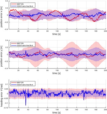
Figure 8 shows estimation error plots for the section of the robot’s trajectory in Fig. 7. Not only does this show the concepts of Bayes space can be applied to a large problem (
 $N$
in the range of thousands) but also that there are some situations where it performs slightly better than the standard MAP Gauss-Newton (GN) algorithm.
Error plots for a portion of the trajectory in the SLAM problem conducted by [Reference Barfoot, Forbes and Yoon14] and discussed in Section 5.3. The exactly sparse Gaussian variational inference (ESGVI) algorithm (red) is equivalent to the iterative projection approach described herein. The maximum a posteriori (MAP) Gauss-Newton (GN) algorithm (blue) is the more standard approach to solving this type of problem. Here, we see ESGVI performing slightly better than MAP GN in terms of smaller errors and more consistency (i.e., errors staying within covariance envelope). Note, in the heading error plot, the red mean line is hidden behind the blue one.

6. Discussion
6.1. Beyond Gaussians
Much of our discussion has centered on projection to the indefinite-Gaussian subspace and also the use of Gaussian measures in our definition of Bayes space. This is primarily because we wanted to show the connection between Bayes space and the Gaussian variational inference framework of [Reference Barfoot, Forbes and Yoon14]. However, we have attempted to lay out the framework to be as general as possible.
As a teaser of applying the methods beyond Gaussians, we can use
 $M \geq 2$
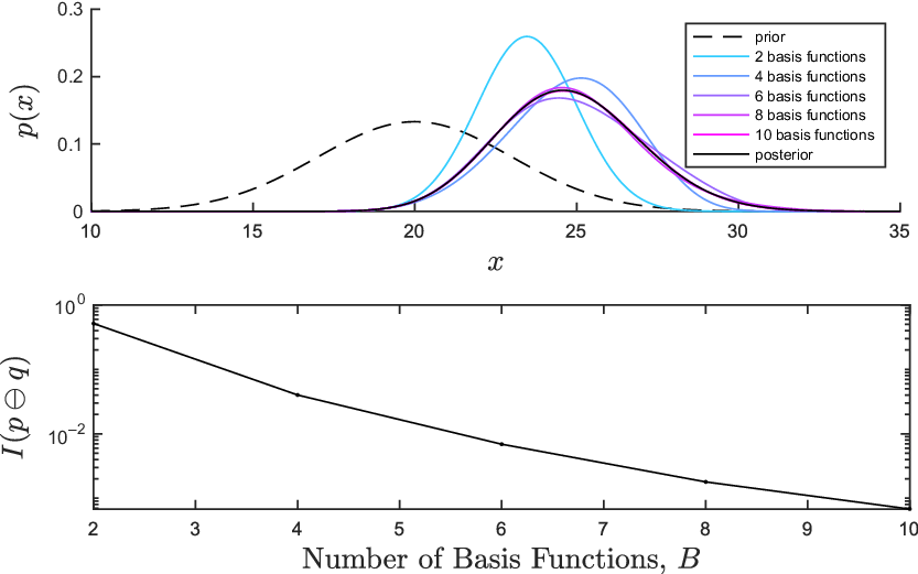
Hermite basis functions to see if we can better approximate a PDF. Figure 9 shows that indeed as we project to a higher-dimensional subspace, we are able to better approximate the stereo camera posterior introduced in Section 3.3. Here we took the measure
 $\nu$
to be equal to the prior for the problem. This shows that even without iteratively updating the measure, we can better approximate the posterior by using more basis functions.
An example of projection of a posterior onto a finite basis with increasing number of basis functions. The top panel qualitatively shows that adding more basis functions brings the approximation closer to the posterior. The bottom shows the same quantitatively where
 $I(p \ominus q)$
decreases exponentially fast with more basis functions. The measure was taken to be the prior in this example.

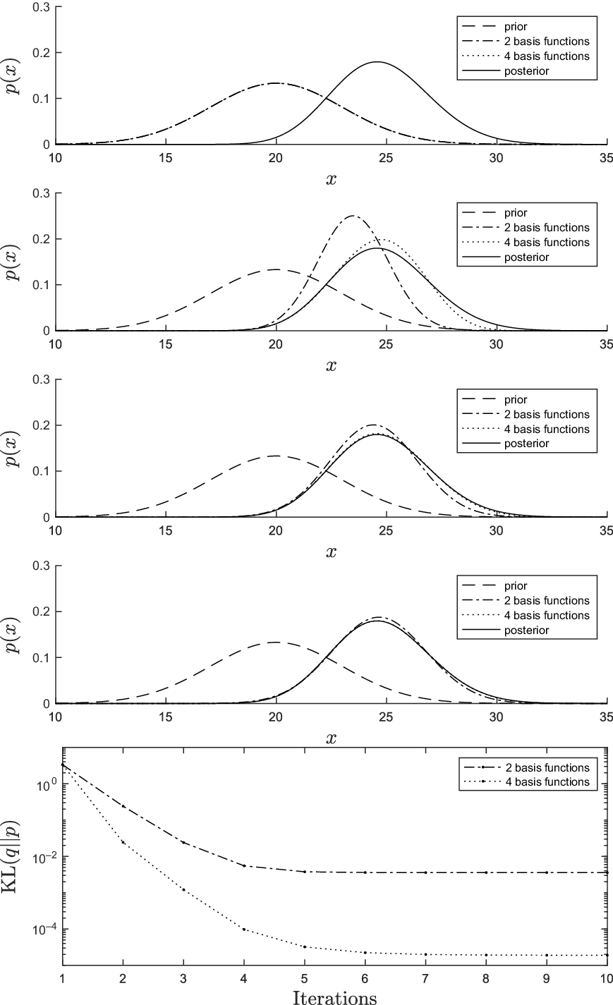
Moreover, we can repeat the iterative projection experiment from Section 4.5, this time with both
 $2$
and
 $4$
basis functions for the approximation. Figure 10 shows the results. We see that the
 $4$
-basis-function estimate requires a few more iterations to converge than the
 $2$
-basis-function one, but it arrives at a better final approximation as demonstrated by the lower final KL divergence.
Example of iterative projection onto subspaces spanned by
 $2$
and
 $4$
Hermite basis functions, where the measure is taken to be the estimate
 $q^{(i)}$
at the previous iteration (projected to the indefinite-Gaussian subspace) and the basis reorthogonalized at each iteration as described in Section 5. The estimates were initialized to the prior (first panel) and then iteratively updated (next three panels). The last panel shows the KL divergence between the estimates and the true posterior for 10 iterations. We see that the estimate using
 $4$
basis functions took slightly longer to converge but in the end produced a better approximation of the posterior.

6.2. Limitations and future work
While the results of the previous section make the use of high-dimensional subspaces look promising, there are some limitations still to overcome, which we discuss here.
First, while the establishment of
 ${\mathcal{B}}^2$
is mathematically sound, it is actually
 $\,\downarrow \!{{\mathcal{B}}^2}$
that we are primarily interested in, since we want to approximate valid PDFs by other valid (simpler) PDFs. It seems through our experiments that we have been lucky in the sense that the results of our projections to Bayesian subspaces are valid PDFs, but there is nothing that actually guarantees this for some of our approximation problems. For example, consider our one-dimensional Gaussian again:
 \begin{equation} p(x) = \underbrace{\left ( -\frac{\mu }{\sigma ^2}\right )}_{\alpha _1} \cdot \underbrace{\exp (\!-x)}_{b_1} \oplus \underbrace{\left (\frac{1}{\sqrt{2}}\frac{1}{\sigma ^2}\right )}_{\alpha _2} \cdot \underbrace{\exp \left ( -\frac{(x^2 - 1)}{\sqrt{2}} \right )}_{b_2} = \alpha _1 \cdot b_1 \oplus \alpha _2 \cdot b_2, \end{equation}
which is a member of
 $\,\downarrow \!{{\mathcal{G}}}$
when
 $\sigma ^2 \gt 0$
. If we project this vector onto
 $\text{span} \{ b_1 \}$
, just the first Hermite basis vector, the result is
 \begin{equation} \underset{\text{span}\left \{ b_1 \right \}}{\text{proj}} \, p = \alpha _1 \cdot b_1, \end{equation}
which is no longer a member of
 $\,\downarrow \!{{\mathcal{G}}}$
since it cannot be normalized to become a valid PDF. Extrapolating from this simple example, it means that truncating a Fourier series at some arbitrary number of terms does not guarantee that the result will be a valid PDF. If we want to extend the Gaussian results to higher-dimensional subspaces, we need to better understand this issue.
Second, even in the case of projecting to the indefinite-Gaussian subspace, guaranteeing that the result is in
 $\,\downarrow \!{{\mathcal{G}}}$
is quite restrictive. If the PDF to be projected is
 \begin{equation} p(\textbf{x}) = c \exp ( -\phi (\textbf{x})), \end{equation}
we saw that the projection to the indefinite-Gaussian subspace (see Appendix D.2) has the form
 \begin{equation} \underset{({\mathcal{G}}, \nu )}{\text{proj}}\, p = \exp \biggl (-(\textbf{x} -{\boldsymbol{\mu }})^T{\mathbb{E}}_\nu \left [\frac{\partial \phi (\textbf{x})}{\partial \textbf{x}^T}\right ] - \frac{1}{2}(\textbf{x} -{\boldsymbol{\mu }})^T \underbrace{{\mathbb{E}}_\nu \left [\frac{\partial ^2\phi (\textbf{x})}{\partial \textbf{x}^T\partial \textbf{x}}\right ]}_{{\boldsymbol{\Sigma }}^{-1}}(\textbf{x} -{\boldsymbol{\mu }})\biggr ), \end{equation}
where we have indicated the resulting inverse covariance is
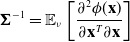 ${\boldsymbol{\Sigma }}^{-1} ={\mathbb{E}}_\nu \left [\dfrac{\partial ^2\phi (\textbf{x})}{\partial \textbf{x}^T\partial \textbf{x}}\right ]$
. To guarantee
 ${\boldsymbol{\Sigma }}^{-1} \gt 0$
which would make this a valid PDF for any choice of the measure
 $\nu$
, we require that
 $\phi (\textbf{x})$
is a convex function of
 $\textbf{x}$
. This is clearly too restrictive for most real estimation problems involving nonlinear measurement models. If
 $\phi (\textbf{x})$
is locally convex, it suggests the measure
 $\nu$
must be chosen so that its probability mass coincides with this region of local convexity. This perhaps emphasizes the need to iteratively update the measure in our proposed projection scheme. However, when the Bayesian posterior and prior are far apart, there is work to be done to understand how best to initialize the measure to ensure the projections wind up in
 $\,\downarrow \!{{\mathcal{B}}^2}$
in the general setup.
Finally, in the general case of projecting to a high-dimensional subspace, the measure itself could also be something other than a Gaussian, depending on the basis that is established. How to carry out the expectations in a computationally efficient and stable way in this case is again future work. The Hermite basis is cooperative in that the basis functions are orthonormal with respect to a Gaussian measure. In the high-dimensional SLAM problem that we discussed in Section 5.3, we (i) exploited sparsity inherent in the problem to require only taking expectations over marginals for each measurement factor, and (ii) were also able to exploit the fact that the measure was Gaussian in order to use Gaussian cubature to carry out the expectations somewhat efficiently [Reference Barfoot, Forbes and Yoon14]. Perhaps there are other bases that could be used for certain problems that admit similar computational conveniences.
It is worth noting that many of the challenges in working with Bayes space stem from the fact that we are attempting to work on infinite domains. If our interest lies with practical robotic state estimation, Bayes space defined over a finite domain [Reference Egozcue, Diaz-Barrero and Pawlowsky-Glahn23] may be both mathematically simpler and more realistic from a practical point of view. This would of course mean giving up on using Gaussians, for example, which could be replaced by a truncated alternative.
7. Concluding remarks
Our principal goal in this work has been to provide a new perspective on the problem of variational inference. This new vantage point is afforded by considering PDFs as elements in a Bayesian Hilbert space, where vector addition is a multiplication (perturbation) that accounts for Bayes’ rule and scalar multiplication is an exponentiation (powering). Gaussians and, more generally, exponential families, which are often used in variational inference, are associated with subspaces. We thus have at our disposal all the familiar instruments of linear algebra.
The use of the KL divergence
 $\text{KL}(q\|p)$
in variational inference to find the best approximation
 $q$
to a given posterior
 $p$
is widespread. In most approaches, the canvas on which the minimization is carried out is a set, usually convex, or a manifold of admissible functions [Reference Adamčík1, Reference Amari3, Reference Amari5, Reference Csiszár20, Reference Csiszár and Tusnády21]. “Projections” of
 $p$
onto the set or manifold are ipso facto the PDF
 $q$
that minimizes the divergence. However, in Bayesian space, we may interpret projections as standard linear-algebraic projections, reminding us of a Euclidean world.
We take particular note of the information geometry of Csiszár and Amari. They along with their colleagues [Reference Amari, Kurata and Nagaoka6, Reference Csiszár and Tusnády21] separately developed the em algorithm—not to be confused with the EM (expectation-maximization) algorithm although the two are in many cases equivalent—to solve the generalized variational problem, which involves a dual minimization of
 $q$
over its manifold and
 $p$
over its own. (The minimum is therefore the minimum “distance” between manifolds.) The e-step of the algorithm is performed by making the manifold “flat,” that is, linear, as a result of using an exponential family of densities. This flattening is equivalent to thinking in terms of a Bayesian space as we have done here. Indeed, as we have shown, the natural-gradient-descent algorithm of [Reference Amari4] can be explained using this framework as a Newton-like iterative projection.
Based on the inner product of our Bayesian space, we have employed an information measure. It is proportional to the squared norm of a probability distribution, which can be used to establish a (symmetric and quadratic) divergence between two PDFs. The connection to the KL divergence is worthwhile mentioning. Each step in the iterative projection algorithm presented here for variational inference based on the KL divergence amounts to a local minimization of our Bayesian-space divergence. Admittedly, our iterative projection approach has some limitations and open issues to resolve. Particularly, we as yet cannot guarantee that the result of a projection will be a valid PDF and hence starting far from the final posterior estimate can pose challenges. We hope others may pick up where we have left off to further develop these ideas and overcome current limitations.
The linear structure of Bayes space furthermore allows us to treat sparsity in measurement data very neatly as the vector sum of the measurements, each of which can be expressed as an element in a subspace restricted to the local variables dictated by the sparsity of the problem, for example, as in the SLAM problem in robotics [Reference Barfoot, Forbes and Yoon14]. The mean-field approximation in variational inference can be handled in much the same way in this framework. The factorization of a distribution with respect to a desired family of distributions would again be rendered as a vector sum of PDFs.
In his fictional autobiography, Zen and the Art of Motorcycle Maintenance, Robert M. Pirsig notes that “One geometry cannot be more true than another; it can only be more convenient.” The same can be said of algebra. Whether one takes a geometric or algebraic tack in analyzing a problem, it can be agreed that different perspectives offer different views and given a particular problem or even a particular class of problem one tack may sometimes be more convenient than others. We hope the perspective presented here on variational inference using a Bayesian Hilbert space offers not only convenience in some respects but insight and a degree of elegance as well.
Authors’ contributions
Barfoot and D’Eleuterio both contributed to the concepts and writing of this work.
Financial support
This work was supported in part by the Natural Sciences and Engineering Research Council of Canada (NSERC).
Conflicts of interest
There are no conflicts of interest, financial or other, for this work.
Ethical considerations
There are no ethical considerations for this work.
Appendix A. Kronecker Product, vec and vech Operators, and Duplication Matrices
For the benefit of the reader, we summarize several identities, which will be used in subsequent appendices, involving the Kronecker product
 $\otimes$
and the vectorization operator
 $\text{vec}(\cdot)$
that stacks the columns of a matrix:
 \begin{equation} \begin{aligned} \text{vec}(\textbf{a}) & \equiv \textbf{a} \\[5pt] \text{vec}(\textbf{a}\textbf{b}^T) & \equiv \textbf{b} \otimes \textbf{a} \\[5pt] \text{vec}(\textbf{A}\textbf{B}\textbf{C}) & \equiv (\textbf{C}^T \otimes \textbf{A} )\, \text{vec}(\textbf{B}) \\[5pt] \text{vec}(\textbf{A})^T \text{vec}(\textbf{B}) & \equiv \text{tr}(\textbf{A}^T\textbf{B}) \\[5pt] (\textbf{A} \otimes \textbf{B})(\textbf{C} \otimes \textbf{D}) & \equiv (\textbf{A}\textbf{C}) \otimes (\textbf{B}\textbf{D}) \\[5pt] (\textbf{A} \otimes \textbf{B})^{-1} & \equiv \textbf{A}^{-1} \otimes \textbf{B}^{-1} \\[5pt] (\textbf{A} \otimes \textbf{B})^{T} & \equiv \textbf{A}^{T} \otimes \textbf{B}^{T}. \end{aligned} \end{equation}
It is worth noting that
 $\otimes$
and
 $\text{vec}(\cdot)$
are linear operators.
As we will be working with (symmetric) covariance matrices when discussing Gaussians, we would like to be able to represent them parsimoniously in terms of only their unique variables. Following [Reference Magnus and Neudecker32, §18], we introduce the half-vectorization operator
 $\text{vech}(\cdot)$
that stacks up the elements in a column matrix, excluding all the elements above the main diagonal. The duplication matrix
 $\textbf{D}$
allows us to recover a full symmetric matrix from its unique parts:
 \begin{equation} \text{vec}(\textbf{A}) = \textbf{D} \, \text{vech}(\textbf{A}) \qquad \text{(symmetric $\textbf{A}$)}. \end{equation}
It is helpful to consider a simple
 $2 \times 2$
example:
 \begin{equation} \textbf{A} = \begin{bmatrix} a\;\;\;\; & b \\[5pt] b\;\;\;\; & c \end{bmatrix}, \quad \text{vec}(\textbf{A}) = \begin{bmatrix} a \\[5pt] b \\[5pt] b \\[5pt] c \end{bmatrix}, \quad \textbf{D} = \begin{bmatrix} 1\;\;\;\; & 0\;\;\;\; & 0\;\;\;\; \\[5pt] 0\;\;\;\; & 1\;\;\;\; & 0 \\[5pt] 0\;\;\;\; & 1\;\;\;\; & 0 \\[5pt] 0\;\;\;\; & 0\;\;\;\; & 1 \end{bmatrix}, \quad \text{vech}(\textbf{A}) = \begin{bmatrix} a \\[5pt] b \\[5pt] c \end{bmatrix}. \end{equation}
The Moore-Penrose pseudoinverse of
 $\textbf{D}$
will be denoted
 $\textbf{D}^\dagger$
and is given by
 \begin{equation} \textbf{D}^\dagger = \left ( \textbf{D}^T \textbf{D} \right )^{-1} \textbf{D}^T. \end{equation}
We can then use
 $\textbf{D}^\dagger$
to convert the vectorization of a matrix into its half-vectorization:
 \begin{equation} \text{vech}(\textbf{A}) = \textbf{D}^\dagger \text{vec}(\textbf{A}) \qquad \text{(symmetric $\textbf{A}$)}. \end{equation}
For our
 $2 \times 2$
example, we have
 \begin{equation} \textbf{D}^\dagger = \begin{bmatrix} 1\;\;\;\; & 0\;\;\;\; & 0\;\;\;\; & 0 \\[5pt] 0\;\;\;\; & \frac{1}{2}\;\;\;\; & \frac{1}{2}\;\;\;\; & 0 \\[5pt] 0\;\;\;\; & 0\;\;\;\; & 0\;\;\;\; & 1\;\;\;\; \end{bmatrix}. \end{equation}
Useful identities involving
 $\textbf{D}$
are then
 \begin{equation} \begin{aligned} \textbf{D}^\dagger \textbf{D} & \equiv \textbf{1} \\[5pt]{\textbf{D}^\dagger }^T \textbf{D}^T & \equiv \textbf{D} \textbf{D}^\dagger \\[5pt] \textbf{D} \textbf{D}^\dagger \text{vec}(\textbf{A}) & \equiv \text{vec}(\textbf{A}) \qquad \qquad \!\text{(symmetric $\textbf{A}$)} \\[5pt] \textbf{D} \textbf{D}^\dagger \left ( \textbf{A} \otimes \textbf{A} \right ) \textbf{D} & \equiv \left ( \textbf{A} \otimes \textbf{A} \right ) \textbf{D} \qquad \text{(any $\textbf{A}$)}, \end{aligned} \end{equation}
which can be found in ref. [Reference Magnus and Neudecker31].
Appendix B. Outer Products
The outer product
 $\Phi :{\mathcal{B}}^2 \rightarrow{\mathcal{B}}^2$
of two vectors
 $b = b(\textbf{x}), c = c(\textbf{x}') \in{\mathcal{B}}^2$
, denoted
 $\Phi (\textbf{x},\textbf{x}') = b(\textbf{x})\rangle \langle c(\textbf{x}')$
or briefly
 $\Phi = b\rangle \langle c$
, is defined by its operation on arbitrary
 $d = d(\textbf{x}') \in{\mathcal{B}}^2$
as
 \begin{equation} \Phi (\textbf{x},\textbf{x}')\circledast d(\textbf{x}') = b(\textbf{x})\rangle \langle c(\textbf{x}')\circledast d(\textbf{x}') = b(\textbf{x}) \cdot \left \langle{c},{d}\right \rangle = \left \langle{c},{d}\right \rangle \cdot b(\textbf{x}). \end{equation}
Thus, dropping the functional dependence,
 \begin{equation} \left \langle{a},{\Phi \circledast d}\right \rangle = \left \langle{a},{b}\right \rangle \left \langle{c},{d}\right \rangle \end{equation}
for arbitrary
 $a \in{\mathcal{B}}^2$
. More generally,
 \begin{equation} \Phi = \bigoplus _{i=1}^M \bigoplus _{j=1}^N \phi _{ij} \cdot b_i\rangle \langle c_j, \end{equation}
where
 $b_i, c_j \in{\mathcal{B}}^2$
and
 $\phi _{ij} \in{\mathbb{R}}$
, so that
 \begin{equation} \Phi \circledast d = \bigoplus _{i=1}^M \sum _{j=1}^N \phi _{ij} \left \langle{c_j},{d}\right \rangle \cdot b_i \end{equation}
and
 \begin{equation} \left \langle{a},{\Phi \circledast d}\right \rangle = \sum _{i=1}^M \sum _{j=1}^N \phi _{ij}\left \langle{a},{b_i}\right \rangle \left \langle{c_j},{d}\right \rangle. \end{equation}
Defining the matrix
 $\boldsymbol{\Phi } = [\phi _{ij}] \in{\mathbb{R}}^{M\times N}$
and
 \begin{equation} \textbf{b}(\textbf{x}) = \begin{bmatrix} b_1(\textbf{x}) \\[5pt] b_2(\textbf{x}) \\[5pt] \vdots \\[5pt] b_M(\textbf{x}) \end{bmatrix}, \quad \textbf{c}(\textbf{x}) = \begin{bmatrix} c_1(\textbf{x}) \\[5pt] c_2(\textbf{x}) \\[5pt] \vdots \\[5pt] c_N(\textbf{x}) \end{bmatrix}, \end{equation}
we may abbreviate (B3) to
 \begin{equation} \Phi (\textbf{x},\textbf{x}') = \textbf{b}(\textbf{x})\rangle \boldsymbol{\Phi }\langle \textbf{c}(\textbf{x}') \end{equation}
and hence
 $ \langle{a},{\Phi \circledast d} \rangle = \boldsymbol{\Phi } \langle \textbf{c},{d} \rangle$
, where
 $ \langle{a},{\textbf{b}} \rangle$
is interpreted as a row and
 $ \langle \textbf{c},{d} \rangle$
as a column.
Given an orthonormal basis
 $\{b_1,b_2\cdots b_M\}$
for a subspace
 ${\mathcal{S}} \subset{\mathcal{B}}^2$
, we define
 \begin{equation} Q = \bigoplus _{m=1}^M b_m\rangle \langle b_m \equiv \textbf{b}\rangle \langle \textbf{b} , \end{equation}
and thus, for any
 $s \in{\mathcal{S}}$
,
 $Q\circledast s = s$
[Reference Manton and Amblard33]. For a nonorthonormal basis,
 \begin{equation} Q = \bigoplus _{m=1}^M \bigoplus _{n=1}^M \kappa _{mn} \cdot b_m \rangle \langle b_n \equiv \textbf{b}\rangle \left \langle{\textbf{b}},{\textbf{b}}\right \rangle ^{-1}\langle \textbf{b}, \end{equation}
where
 $\kappa _{mn}$
is the
 $(m,n)$
entry in
 $ \langle{\textbf{b}},{\textbf{b}} \rangle ^{-1}$
. Notationally,
 $\cdot \rangle \textbf{A} \langle \cdot$
indicates an outer product weighted in the middle by an appropriately sized matrix
 $\textbf{A}$
, which in the above example serves to normalize the basis. In normal matrix algebra, it would be equivalent, for example, to writing
 $\textbf{a} (\textbf{a}^T\textbf{a})^{-1} \textbf{a}^T$
, for some column
 $\textbf{a}$
.
Using the outer product, we can write a projection as
 \begin{equation} q^\star (\textbf{x}) = Q(\textbf{x},\textbf{x}')\circledast p(\textbf{x}'), \end{equation}
where
 \begin{equation} Q(\textbf{x},\textbf{x}') = \textbf{b}(\textbf{x})\rangle \left \langle{\textbf{b}},{\textbf{b}}\right \rangle ^{-1} \langle \textbf{b}(\textbf{x}'), \end{equation}
which plays a similar role to projection matrix.
Appendix C. Hermite Basis
C.1. Basis for
 $\mathbb{R}$

Consider the domain over which members of
 ${\mathcal{B}}^2$
are defined to be
 $\mathbb{R}$
. We can use the exponentiated Hermite polynomials as a basis for our infinite-dimensional
 ${\mathcal{B}}^2$
; in fact, they prove to be a natural choice [Reference van den Boogaart, Egozcue and Pawlowsky-Glahn43]. In one dimension, the first few probabilist’s Hermite polynomials are
 \begin{equation} H_1(\xi ) = \xi, \quad H_2(\xi ) = \xi ^2-1, \quad H_3(\xi ) = \xi ^3-3\xi, \quad H_4(\xi ) = \xi ^4-6\xi ^2+3. \end{equation}
(We exclude
 $H_0(\xi ) = 1$
as the resulting vector is the zero vector; however, it will need to be introduced when considering the domain
 ${\mathbb{R}}^N$
as explained in Appendix C.2.) Owing to the properties of the Hermite polynomials, namely, that
 \begin{equation} \int _{-\infty }^{\infty } H_n(\xi )\nu (\xi )\, d\xi = 0, \quad \int _{-\infty }^{\infty } H_m(\xi ) H_n(\xi ) \nu (\xi )\, d\xi = n!\,{\delta }_{mn}, \,\, m,n=1,2,3\ldots, \end{equation}
where
 $\nu (\xi ) = \mathcal{N}(0,1)$
is the standard normal density, we can construct an orthonormal basis for
 ${\mathcal{B}}^2$
following [Reference Egozcue, Diaz-Barrero and Pawlowsky-Glahn23]. Accordingly,
 \begin{equation} \mathbb{E}_\nu [H_n] = 0, \quad \mathbb{E}_\nu [H_m H_n] = n!\,\delta _{mn}, \quad m,n = 1, 2, 3\ldots \end{equation}
Our basis functions are
 \begin{equation} h_n(\xi ) =\exp \left (-\eta _n(\xi )\right ), \quad \eta _n(\xi ) = \frac{1}{\sqrt{n!}} H_n(\xi ). \end{equation}
Orthogonality follows as
 \begin{align} \left \langle{h_m},{h_n}\right \rangle & = \mathbb{E}_\nu \!\left [ \eta _m \eta _n \right ] -{\mathbb{E}}_\nu \left [ \eta _m \right ] \mathbb{E}_\nu \!\left [ \eta _n \right ]\nonumber \\[5pt] & = \frac{1}{\sqrt{m!n!}} \int _{-\infty }^\infty H_m(\xi ) H_n(\xi ) \frac{1}{\sqrt{2\pi }}\exp \left (\!-\frac{1}{2} \xi ^2\right )\, d\xi = \delta _{mn}. \end{align}
An arbitrary member
 $p$
of
 ${\mathcal{B}}^2$
can be expanded in terms of this Hermite basis. However, we first need two lemmata, resting on the recursive definition of Hermite polynomials; these are
Lemma C.1.
For the standard normal measure,
 $\nu \sim \mathcal{N}(0,1)$
,
 \begin{equation} \mathbb{E}_\nu \!\left [ H_{n+1}(\xi ) f(\xi ) \right ] = \mathbb{E}_\nu \!\left [ H_n(\xi ) \frac{\partial f(\xi )}{\partial \xi } \right ]. \end{equation}
where
 $f(\xi )$
is a differentiable function and is such that the expectations exist.
Proof. The
 $n=0$
case,
 \begin{equation} \mathbb{E}_\nu \!\left [ \xi f \right ] = \mathbb{E}_\nu \!\left [ \frac{\partial f}{\partial \xi } \right ], \end{equation}
is immediately true by Stein’s lemma [Reference Stein40]. For general case
 $n$
,
 \begin{align} \mathbb{E}_\nu \!\left [H_{n+1} f \right ] = \mathbb{E}_\nu\! \left [\left ( \xi H_n - \frac{\partial H_n}{\partial \xi } \right ) f \right ] = \mathbb{E}_\nu \!\left [\frac{\partial }{\partial \xi } \left (H_n f \right ) - \frac{\partial H_n}{\partial \xi } f \right ] & = \mathbb{E}_\nu \!\left [\frac{\partial H_n}{\partial \xi } f + H_n \frac{\partial f}{\partial \xi }- \frac{\partial H_n}{\partial \xi } f \right ]\nonumber \\[5pt] & = \mathbb{E}_\nu \!\left [H_n \frac{\partial f}{\partial \xi } \right ], \end{align}
where we have used the recurrence relation,
 \begin{equation} H_{n+1} = \xi H_n - \frac{\partial H_n}{\partial \xi }, \end{equation}
for the Hermite polynomials.
Lemma C.2.
For the standard normal measure,
 $\nu \sim \mathcal{N}(0,1)$
,
 \begin{equation} \mathbb{E}_\nu \!\left [ H_n(\xi ) f(\xi ) \right ] = \mathbb{E}_\nu \!\left [\frac{\partial ^n f(\xi )}{\partial \xi ^n} \right ], \end{equation}
where
 $f(\xi )$
is an
 $n$
-fold differentiable function and is such that the expectations exist.
Proof. Repeatedly applying Lemma C.1,
 \begin{align} \mathbb{E}_\nu \!\left [ H_n f \right ] = \mathbb{E}_\nu \!\left [ H_{n-1} \frac{\partial f}{\partial \xi } \right ] = \mathbb{E}_\nu \!\left [ H_{n-2} \frac{\partial ^2 f}{\partial \xi ^2} \right ] = \cdots = \mathbb{E}_\nu \!\left [ H_{1} \frac{\partial ^{n-1} f}{\partial \xi ^{n-1}} \right ] = \mathbb{E}_\nu \!\left [ H_0\frac{\partial ^n f}{\partial \xi ^n} \right ] = \mathbb{E}_\nu \!\left [\frac{\partial ^n f}{\partial \xi ^n} \right ], \end{align}
yields the desired result.
Now consider any
 $p \in{\mathcal{B}}^2$
expressed as
 $p(\xi ) = c\exp (\!-\phi (\xi ))$
. The coordinates are given by
 \begin{equation} \alpha _n = \left \langle{h_n},{p}\right \rangle = \frac{1}{\sqrt{n!}}{{\mathbb{E}}}_\nu \left [\frac{\partial ^n \phi (\xi )}{\partial \xi ^n} \right ] \end{equation}
and hence
 \begin{equation} p(\xi ) = \bigoplus _{n=1}^\infty \alpha _n\cdot h_n(\xi ) = \exp \left (\!-\sum _{n=1}^\infty \frac{1}{n!}{{\mathbb{E}}}_\nu \left [\frac{\partial ^n\phi (\xi )}{\partial \xi ^n}\right ]H_n(\xi )\right ). \end{equation}
We can account for measures other than the standard normal density, say
 $\nu \sim{\mathcal{N}}(\mu,\sigma ^2)$
, by the well-known reparameterization “trick,”
 \begin{equation} x = \mu + \sigma \xi, \end{equation}
which leads to
 \begin{equation} p(x) = \bigoplus _{n=1}^\infty \alpha _n \cdot h_n\left (\frac{x-\mu }{\sigma }\right ) = \exp \left ( - \sum _{n=1}^\infty \frac{\sigma ^n}{n!} \mathbb{E}_\nu \!\left [\frac{\partial ^n \phi (x)}{\partial x^n} \right ] H_n\left (\frac{x-\mu }{\sigma }\right )\right ). \end{equation}
It is instructive to rewrite this expression by replacing
 $-\phi$
with
 $\ln p$
giving
 \begin{equation} p(x) = \exp \left ( \sum _{n=1}^\infty \frac{\sigma ^n}{n!} \mathbb{E}_\nu \!\left [\frac{\partial ^n \ln p(x)}{\partial x^n} \right ] H_n\left (\frac{x-\mu }{\sigma }\right )\right ). \end{equation}
This is a Taylor-like expansion of
 $p$
pivoting on a given mean
 $\mu$
and standard deviation
 $\sigma$
.
Any subset of the basis functions
 $\{h_1, h_2, \ldots \}$
establishes a subspace of
 ${\mathcal{B}}^2$
; however, as far as such subspaces are concerned, it would be natural to choose an
 $M$
-dimensional subspace
 $\mathcal{H}$
spanned by the first
 $M$
basis functions. As the basis is orthonormal, the Gram matrix is
 $ \langle{\textbf{h}},{\textbf{h}} \rangle = \textbf{1}$
.
The Hermite functions can also be used to generate a basis for
 ${\mathcal{B}}^2$
on the domain
 ${\mathbb{R}}^N$
, which we detail in the next subsection.
C.2. Basis for
$\boldsymbol{{\mathbb{R}}^N}$

We can extend the results of the previous subsection to create a Hermite basis for
 ${\mathcal{B}}^2$
on
 ${\mathbb{R}}^N$
. Let
 \begin{equation}{\boldsymbol{\eta }}(\xi ) = \frac{1}{\sqrt{n!}} \begin{bmatrix} H_0(\xi ) \\[5pt] H_1(\xi ) \\[5pt] \vdots \\[5pt] H_M(\xi ) \end{bmatrix}. \end{equation}
Note that we have reintroduced
 $H_0(\xi )$
because the basis will be created by all possible combinatorial
 $N$
-products of these functions, one for each variable in
 ${\boldsymbol{\xi }} \in{\mathbb{R}}^N$
. However, we will have to exclude the combination made up of only
 $H_0$
because once again this function gives the zero vector of
 ${\mathcal{B}}^2$
. We may express this operation as a Kronecker product, that is,
 \begin{equation}{\boldsymbol{\eta }}({\boldsymbol{\xi }}) = \textbf{C}\left ({\boldsymbol{\eta }}(\xi _1)\otimes{\boldsymbol{\eta }}(\xi _2)\otimes \cdots \otimes{\boldsymbol{\eta }}(\xi _N)\right ), \end{equation}
where
 $\textbf{C} = [\,\textbf{0}\;\;\textbf{1}\,]$
contains zero in the first column followed by the identity matrix; this removes the offending function. Observe that
 $\textbf{C}\textbf{C}^T = \textbf{1}$
. The basis is then
 \begin{equation} \textbf{h}({\boldsymbol{\xi }}) = \exp (\!-\!{\boldsymbol{\eta }}({\boldsymbol{\xi }})). \end{equation}
The total number of basis functions is
 $(M + 1)^N - 1$
.
This set of basis functions retains its orthonormality because
 \begin{align*} & \left \langle{\textbf{h}({\boldsymbol{\xi }})},{\textbf{h}({\boldsymbol{\xi }})}\right \rangle = \mathbb{E}_\nu \!\left [ \left (\textbf{C}{\boldsymbol{\eta }}(\xi _1) \otimes \cdots \otimes{\boldsymbol{\eta }}(\xi _N) \right ) \left (\textbf{C}{\boldsymbol{\eta }}(\xi _1) \otimes \cdots \otimes{\boldsymbol{\eta }}(\xi _N) \right )^T \right ] \\[5pt] &\quad\quad\quad\quad\quad\quad\quad\quad\quad\quad\quad\quad\quad\quad\quad\quad\quad\quad\quad\quad = \textbf{C} \, \mathbb{E}_\nu \!\left [{\boldsymbol{\eta }}(\xi _1){\boldsymbol{\eta }}(\xi _1)^T \otimes \cdots \otimes{\boldsymbol{\eta }}(\xi _N){\boldsymbol{\eta }}(\xi _N)^T \right ]\textbf{C}^T \end{align*}
by a property of the Kronecker product (Appendix A). Now
 \begin{align} & \mathbb{E}_\nu \!\left [{\boldsymbol{\eta }}(\xi _1){\boldsymbol{\eta }}(\xi _1)^T \otimes \cdots \otimes{\boldsymbol{\eta }}(\xi _N){\boldsymbol{\eta }}(\xi _N)^T \right ] \\[5pt] &\quad\quad\quad\quad\quad\quad = \int _{-\infty }^\infty{\boldsymbol{\eta }}(\xi _1){\boldsymbol{\eta }}(\xi _1)^T \nu (\xi _1)\, d\xi _1 \otimes \cdots \otimes \int _{-\infty }^\infty{\boldsymbol{\eta }}(\xi _N){\boldsymbol{\eta }}(\xi _N)^T \nu (\xi _N)\, d\xi _N = \textbf{1}_{(M + 1)^N\times (M + 1)^N}, \end{align}
wherein each of the integrals expresses the orthonormality of the Hermite functions and results in an
 $(M + 1)\times (M + 1)$
identity matrix. Hence
 \begin{equation} \left \langle{\textbf{h}({\boldsymbol{\xi }})},{\textbf{h}({\boldsymbol{\xi }})}\right \rangle = \textbf{C} \, \textbf{1}_{(M + 1)^N\times (M + 1)^N}\textbf{C}^T = \textbf{1}_{[(M+1)^N-1]\times [(M+1)^N-1]}. \end{equation}
To determine the coordinates of an arbitrary
 $p \in{\mathcal{B}}^2$
, we shall require the multivariate version of Lemma 2:
Lemma C.3.
For the standard normal measure,
 $\nu \sim \mathcal{N}(\textbf{0},\textbf{1})$
,
 \begin{equation} \mathbb{E}_\nu \!\left [ H_{n_1}(\xi _1)H_{n_2}(\xi _2)\cdots H_{n_N}(\xi _N) f({\boldsymbol{\xi }}) \right ] = \mathbb{E}_\nu \!\left [\frac{\partial ^{n_1+n_2 + \cdots + n_N} f({\boldsymbol{\xi }})}{\partial \xi _1^{n_1}\partial \xi _2^{n_2}\cdots \partial \xi _N^{n_N}} \right ], \quad \quad n_k = 1, 2\cdots M. \end{equation}
where
 $f\;:\;{\mathbb{R}}^N \rightarrow{\mathbb{R}}$
is
 $n_k$
-fold differentiable in
 $\xi _k$
and is such that the expectations exist.
The proof relies on the use of Lemma 2 for each individual partial derivative; for example, with respect to the variable
 $\xi _1$
,
 \begin{equation} \mathbb{E}_\nu \bigl [ H_{n_1}(\xi _1)H_{n_2}(\xi _2)\cdots H_{n_N}(\xi _N) f({\boldsymbol{\xi }}) \bigr ] = \mathbb{E}_\nu \!\left [ H_{n_1-1}(\xi _1)H_{n_2}(\xi _2)\cdots H_{n_N}(\xi _N) \frac{\partial f({\boldsymbol{\xi }})}{\partial \xi _1} \right ]. \end{equation}
The product
 $H_{n_1}(\xi _2)\cdots H_{n_N}(\xi _N)$
has no dependence on
 $\xi _1$
and can therefore be treated as a constant. Doing the same for all the other variables and for the indicated number of times leads to the stated result.
We can streamline the notation by defining
 \begin{equation}{\boldsymbol{\partial }}_\xi = \begin{bmatrix} 1 & \dfrac{ \partial }{ \partial \xi } & \dfrac{ \partial ^2}{ \partial \xi ^2} & \cdots & \dfrac{ \partial ^M}{ \partial \xi ^M} \end{bmatrix} \end{equation}
and, as above,
 \begin{equation}{\boldsymbol{\partial }}_{{\boldsymbol{\xi }}} = \textbf{C}({\boldsymbol{\partial }}_{\xi _1} \otimes{\boldsymbol{\partial }}_{\xi _2} \otimes \cdots \otimes{\boldsymbol{\partial }}_{\xi _N}). \end{equation}
Using the measure
 $\nu ={\mathcal{N}}(0,1)$
, then,
 \begin{equation} \boldsymbol \alpha = \left \langle{\textbf{h}({\boldsymbol{\xi }})},{p({\boldsymbol{\xi }})}\right \rangle ={\mathbb{E}}_\nu [{\boldsymbol{\partial }}_{{\boldsymbol{\xi }}}p({\boldsymbol{\xi }})] \end{equation}
are the coordinates of
 $p({\boldsymbol{\xi }}) \in{\mathcal{B}}^2$
, truncated to however many basis functions we decide to keep.
Appendix D. Multivariate Gaussians
D.1. Basis for multivariate Gaussians
Multivariate Gaussians are quintessentially important to statistics and estimation theory. Gaussians, as traditionally defined with a positive-definite covariance matrix, do not in themselves form a subspace of
 ${\mathcal{B}}^2$
. We need to expand the set to include covariance matrices that are sign-indefinite. Let us accordingly define an
 $N$
-dimensional indefinite-Gaussian PDF as
 \begin{equation} p(\textbf{x}) = c \exp \left ( -\frac{1}{2} (\textbf{x} -{\boldsymbol{\mu }})^T \boldsymbol{\Sigma }^{-1} (\textbf{x} -{\boldsymbol{\mu }}) \right ), \end{equation}
which has mean,
 $\boldsymbol{\mu }$
, and symmetric covariance,
 $\boldsymbol{\Sigma }$
. The set of all
 $N$
-dimensional, indefinite Gaussians is
 \begin{equation}{\mathcal{G}} = \left \{ p(\textbf{x}) = c\exp \left ( -\frac{1}{2} (\textbf{x} -{\boldsymbol{\mu }})^T \boldsymbol{\Sigma }^{-1} (\textbf{x} -{\boldsymbol{\mu }}) \right ) \, \biggl | \,{\boldsymbol{\mu }} \in \mathbb{R}^N, \boldsymbol{\Sigma } \in \mathbb{R}^{N \times N}, 0 \lt c \lt \infty \right \}. \end{equation}
It is easy to show that
 $\mathcal{G}$
is in fact a subspace of
 ${\mathcal{B}}^2$
as the zero vector is contained therein (
 $\boldsymbol{\Sigma }^{-1} = \textbf{O}$
, allowing that
 $\boldsymbol{\Sigma } \rightarrow \infty$
) and the set is closed under vector addition and scalar multiplication.
To establish
 $\mathcal{G}$
as a Bayesian Hilbert space, we must have an appropriate measure,
 $\nu$
. In our case, we choose the measure to also be a Gaussian,
 $\nu = \mathcal{N} ({\boldsymbol{\mu }}, \boldsymbol{\Sigma } ) \in{\mathcal{G}}$
. We may thus declare
 $\mathcal{G}$
to be a Bayesian Hilbert space for a measure
 $\nu \in{\mathcal{G}}$
. We will refer to the set of Gaussian PDFs with positive-definite covariance,
 ${\boldsymbol{\Sigma }} \gt 0$
, as
 $\,\downarrow \!{{\mathcal{G}}} \subset{\mathcal{G}}$
.
Several possibilities exist to parameterize Gaussians [Reference Barfoot11]. There are
 $\frac{1}{2}N(N + 3)$
unique elements contained in the mean and the symmetric covariance matrix on
 ${\mathbb{R}}^N$
; hence the dimension of
 $\mathcal{G}$
is
 $\frac{1}{2}N(N + 3)$
. We shall construct our basis on a positive-definite choice of covariance
 $\boldsymbol{\Sigma }$
that we can decompose in Cholesky fashion, that is,
 $\boldsymbol{\Sigma } = \textbf{L}\textbf{L}^T$
. Now consider
 \begin{equation} {\boldsymbol{\gamma }}_1(\textbf{x}) = \textbf{L}^{-1}(\textbf{x} -{\boldsymbol{\mu }}), \quad{\boldsymbol{\gamma }}_2(\textbf{x}) = \sqrt{\text{$\frac{1}{2}$}\textbf{D}^T\textbf{D}}\,\text{vech}\,(\textbf{L}^{-1}(\textbf{x} -{\boldsymbol{\mu }})(\textbf{x} -{\boldsymbol{\mu }})^T\textbf{L}^{-T}), \end{equation}
wherein
 $\text{vech}\,(\cdot)$
is the half-vectorization of its matrix argument and
 $\textbf{D}$
is the associated duplication matrix (see Appendix A). Note that
 ${\boldsymbol{\gamma }}_1$
is an
 $N\times 1$
column and
 ${\boldsymbol{\gamma }}_2$
is an
 $\frac{1}{2}N(N + 1)\times 1$
column. With a little abuse of notation, we set the basis functions as
 \begin{equation} \textbf{g}(\textbf{x}) = \begin{bmatrix} \textbf{g}_1(\textbf{x}) \\[5pt] \textbf{g}_2(\textbf{x}) \end{bmatrix} = \exp \left (\!- \begin{bmatrix}{\boldsymbol{\gamma }}_1(\textbf{x}) \\[5pt]{\boldsymbol{\gamma }}_2(\textbf{x}) \end{bmatrix}\right ); \end{equation}
that is, the exponential is applied elementwise. We claim that
 $\textbf{g}(\textbf{x})$
is a basis for
 $\mathcal{G}$
.
It is instructive to show that
 $\textbf{g}(\textbf{x})$
spans
 $\mathcal{G}$
as well as serving as the proof that it is a basis. Consider again the reparameterization “trick” given by
 \begin{equation} \textbf{x} ={\boldsymbol{\mu }} + \textbf{L}{\boldsymbol{\xi }} \end{equation}
with
 ${\boldsymbol{\xi }} \sim{\mathcal{N}}(\textbf{0},\textbf{1})$
. This renders (D4) as
 \begin{equation} \textbf{g}({\boldsymbol{\xi }}) = \begin{bmatrix} \textbf{g}_1({\boldsymbol{\xi }}) \\[5pt] \textbf{g}_2({\boldsymbol{\xi }}) \end{bmatrix} = \exp \left (\!- \begin{bmatrix}{\boldsymbol{\gamma }}_1({\boldsymbol{\xi }}) \\[5pt]{\boldsymbol{\gamma }}_2({\boldsymbol{\xi }})\end{bmatrix}\right ) = \exp \left (\!- \begin{bmatrix}{\boldsymbol{\xi }} \\[5pt]\sqrt{\text{$\frac{1}{2}$}\textbf{D}^T\textbf{D}}\,\text{vech}\,{\boldsymbol{\xi }}{\boldsymbol{\xi }}^T \end{bmatrix}\right ). \end{equation}
A (normalized) linear combination of the basis functions can be written as
 \begin{equation} p({\boldsymbol{\xi }}) = \,\downarrow \!{\exp }\left (\!-\boldsymbol \alpha _1^T{\boldsymbol{\gamma }}_1({\boldsymbol{\xi }}) - \boldsymbol \alpha _2^T{\boldsymbol{\gamma }}_2({\boldsymbol{\xi }})\right ). \end{equation}
Now
 \begin{equation} \boldsymbol \alpha _1^T{\boldsymbol{\gamma }}_1 = \boldsymbol \alpha _1^T{\boldsymbol{\xi }}. \end{equation}
Also, we can in general express the second set of coordinates as
 \begin{equation} \boldsymbol \alpha _2 =\sqrt{\text{$\frac{1}{2}$}\textbf{D}^T\textbf{D}}\;\text{vech}\,\textbf{S} \end{equation}
for some symmetric
 $\textbf{S}$
that can easily be reconstructed from
 $\boldsymbol \alpha _2$
. Hence
 \begin{equation} \boldsymbol \alpha _2^T{\boldsymbol{\gamma }}_2 = \frac{1}{2}(\text{vech}\;\textbf{S})^T\textbf{D}^T\textbf{D}\text{vech}\,{\boldsymbol{\xi }}{\boldsymbol{\xi }}^T = \frac{1}{2}(\text{vec}\,\textbf{S})^T\text{vec}\,{\boldsymbol{\xi }}{\boldsymbol{\xi }}^T \end{equation}
given the identities
 $\text{vech}\,\textbf{A} = \textbf{D}^\dagger \text{vec}\,\textbf{A}$
and
 $\textbf{DD}^\dagger \text{vec}\,\textbf{A} = \text{vec}\,\textbf{A}$
, where
 $\textbf{D}^\dagger$
is the Moore-Penrose inverse of
 $\textbf{D}$
(Appendix A). Moreover, the identity
 $(\text{vec}\,\textbf{A})^T\text{vec}\,\textbf{b} = \text{tr}\,\textbf{AB}$
leads to
 \begin{equation} \boldsymbol \alpha _2^T{\boldsymbol{\gamma }}_2 = \frac{1}{2}\text{tr}\left (\textbf{S}{\boldsymbol{\xi \xi }}^T\right ) = \frac{1}{2}{\boldsymbol{\xi }}^T\textbf{S}{\boldsymbol{\xi }}. \end{equation}
Then
 \begin{align*} & p(\textbf{x}) = \,\downarrow \!{\exp }\left (\!-\boldsymbol \alpha _1^T{\boldsymbol{\xi }} - \frac{1}{2}{\boldsymbol{\xi }}^T\textbf{S}{\boldsymbol{\xi }}\right ) = \,\downarrow \!{\exp }\left (\!-\frac{1}{2}\left ({\boldsymbol{\xi }} + \textbf{S}^{-1} \boldsymbol \alpha _1)^T\textbf{S}({\boldsymbol{\xi }} + \textbf{S}^{-1} \boldsymbol \alpha _1\right )\right ) \\[5pt] & \quad\quad\quad\quad\quad\quad\quad\quad\quad\quad\quad = \,\downarrow \!{\exp }\left (\!-\frac{1}{2}\left (\textbf{x} - ({\boldsymbol{\mu }} - \textbf{L} \textbf{S}^{-1}\boldsymbol \alpha _1)\right )^T\textbf{L}^{-T}\textbf{S}\textbf{L}^{-1}\left (\textbf{x} - ({\boldsymbol{\mu }} - \textbf{L} \textbf{S}^{-1}\boldsymbol \alpha _1)\right )\right ). \end{align*}
This can represent any Gaussian distribution, where the mean is
 ${\boldsymbol{\mu }} - \textbf{L} \textbf{S}^{-1}\boldsymbol \alpha _1$
and the covariance
 $\textbf{LS}^{-1}\textbf{L}^T$
. Thus,
 $\textbf{g}$
spans
 $\mathcal{G}$
. Furthermore, as the dimension of
 $\mathcal{G}$
is
 $\frac{1}{2}N(N + 3)$
, the number of functions in
 $\textbf{g}$
,
 $\textbf{g}$
is a basis for
 $\mathcal{G}$
.
This basis is, in addition, orthonormal as can be proven in a straightforward fashion by using the reparameterized form
 $\textbf{g}({\boldsymbol{\xi }})$
and recognizing that the entries in
 ${\boldsymbol{\gamma }}_1({\boldsymbol{\xi }})$
are
 $\xi _i$
and those in
 ${\boldsymbol{\gamma }}_2({\boldsymbol{\xi }})$
are either
 $\xi _i\xi _j$
(
 $i\not =j$
) or
 $\xi _i^2/\sqrt{2}$
. Hence,
 $ \langle{\textbf{g}},{\textbf{g}} \rangle = \textbf{1}$
.
It can be shown that
 \begin{align} \boldsymbol \alpha _1 &= \left \langle{\textbf{g}_1},{p}\right \rangle = \textbf{L}^T{\mathbb{E}}_\nu \left [\frac{\partial \phi (\textbf{x})}{\partial \textbf{x}^T}\right ], \nonumber \\[5pt] \boldsymbol \alpha _2 &= \left \langle{\textbf{g}_2},{p}\right \rangle = \sqrt{\text{$\frac{1}{2}$}\textbf{D}^T\textbf{D}}\, \text{vech}\left (\textbf{L}^T{\mathbb{E}}_\nu \left [\frac{\partial ^2\phi (\textbf{x})}{\partial \textbf{x}^T\partial \textbf{x}}\right ]\textbf{L}\right ) \end{align}
are the coordinates for
 $p(\textbf{x}) = \,\downarrow \!{\exp (\!-\phi (\textbf{x}))} \in{\mathcal{G}}$
. Another rendering of (D12) is
 \begin{equation} p(\textbf{x}) = \,\downarrow \!{\exp }\left (\!-(\textbf{x} -{\boldsymbol{\mu }})^T{\mathbb{E}}_\nu \left [\frac{\partial \phi (\textbf{x})}{\partial \textbf{x}^T}\right ] - \frac{1}{2}(\textbf{x} -{\boldsymbol{\mu }})^T{\mathbb{E}}_\nu \left [\frac{\partial ^2\phi (\textbf{x})}{\partial \textbf{x}^T\partial \textbf{x}}\right ](\textbf{x} -{\boldsymbol{\mu }})\right ), \end{equation}
which also expresses the projection of a PDF in
 ${\mathcal{B}}^2$
onto
 $\mathcal{G}$
.
D.2. Coordinates of multivariate Gaussian projection
Let
 $p(\textbf{x}) = c \exp ( -\phi (\textbf{x})) \in{\mathcal{B}}^2$
. Projecting onto
 $\mathcal{G}$
, the coordinates associated with basis functions
 $\textbf{g}_1$
are
 \begin{eqnarray}{\boldsymbol{\alpha }}_1 & = & \left \langle{\textbf{g}_1},{p}\right \rangle \nonumber \\[7pt] & = & \mathbb{E}_\nu \!\left [{\boldsymbol{\gamma }}_1(\textbf{x}) \phi (\textbf{x}) \right ] - \mathbb{E}_\nu \!\left [{\boldsymbol{\gamma }}_1(\textbf{x}) \right ] \mathbb{E}_\nu \!\left [ \phi (\textbf{x}) \right ] \nonumber \\[7pt] & = & \mathbb{E}_\nu \!\left [ \textbf{L}^{-1} (\textbf{x} -{\boldsymbol{\mu }}) \phi (\textbf{x}) \right ] - \underbrace{\mathbb{E}_\nu \!\left [ \textbf{L}^{-1} (\textbf{x} -{\boldsymbol{\mu }})\right ]}_{\textbf{0}} \mathbb{E}_\nu \!\left [ \phi (\textbf{x}) \right ] \\[7pt] & = & \textbf{L}^{-1} \boldsymbol{\Sigma } \, \mathbb{E}_\nu \!\left [ \frac{\partial \phi (\textbf{x})}{\partial \textbf{x}^T}\right ] \nonumber \\[7pt] & = & \textbf{L}^{T} \mathbb{E}_\nu \!\left [ \frac{\partial \phi (\textbf{x})}{\partial \textbf{x}^T}\right ], \nonumber \end{eqnarray}
where we have employed Stein’s lemma [Reference Stein40] to go from the third line to the fourth. Taking the inner product of these coefficients with the associated basis functions, we have
 \begin{equation}{\boldsymbol{\alpha }}_1^T{\boldsymbol{\gamma }}_1(\textbf{x}) = \mathbb{E}_\nu \!\left [ \frac{\partial \phi (\textbf{x})}{\partial \textbf{x}^T}\right ]^T \textbf{L} \textbf{L}^{-1} (\textbf{x} -{\boldsymbol{\mu }}) = \mathbb{E}_\nu \!\left [ \frac{\partial \phi (\textbf{x})}{\partial \textbf{x}^T}\right ] ^T (\textbf{x} -{\boldsymbol{\mu }}). \end{equation}
The coordinates associated with basis functions
 $\textbf{g}_2$
are
 \begin{eqnarray}{\boldsymbol{\alpha }}_2 & = & \left \langle{\textbf{g}_2},{p}\right \rangle \nonumber \\[7pt] & = & \mathbb{E}_\nu \!\left [{\boldsymbol{\gamma }}_2(\textbf{x}) \phi (\textbf{x}) \right ] - \mathbb{E}_\nu \!\left [{\boldsymbol{\gamma }}_2(\textbf{x}) \right ] \mathbb{E}_\nu \!\left [ \phi (\textbf{x}) \right ] \nonumber \\[7pt] & = & \mathbb{E}_\nu \!\left [\sqrt{\text{$\frac{1}{2}$}\textbf{D}^T\textbf{D}} \text{vech}\left ( \textbf{L}^{-1} (\textbf{x} -{\boldsymbol{\mu }})(\textbf{x} -{\boldsymbol{\mu }})^T \textbf{L}^{-T} \right ) \phi (\textbf{x}) \right ] \nonumber \\[7pt] & & \qquad - \; \mathbb{E}_\nu \!\left [ \sqrt{\text{$\frac{1}{2}$}\textbf{D}^T\textbf{D}} \text{vech}\left ( \textbf{L}^{-1} (\textbf{x} -{\boldsymbol{\mu }})(\textbf{x} -{\boldsymbol{\mu }})^T \textbf{L}^{-T} \right ) \right ] \mathbb{E}_\nu \!\left [ \phi (\textbf{x}) \right ] \\[7pt] & = & \sqrt{\text{$\frac{1}{2}$}\textbf{D}^T\textbf{D}} \text{vech}\left ( \textbf{L}^{-1} \left (\mathbb{E}_\nu \!\left [ (\textbf{x} -{\boldsymbol{\mu }})(\textbf{x} -{\boldsymbol{\mu }})^T \phi (\textbf{x}) \right ] - \boldsymbol{\Sigma } \mathbb{E}_\nu \!\left [\phi (\textbf{x})\right ] \right ) \textbf{L}^{-T} \right ) \nonumber \\[7pt] & = & \sqrt{\text{$\frac{1}{2}$}\textbf{D}^T\textbf{D}} \text{vech}\left ( \textbf{L}^{-1} \boldsymbol{\Sigma } \, \mathbb{E}_\nu \!\left [ \frac{\partial ^2 \phi (\textbf{x})}{\partial \textbf{x}^T \partial \textbf{x}} \right ] \boldsymbol{\Sigma } \textbf{L}^{-T} \right ) \nonumber \\[7pt] & = &\sqrt{\text{$\frac{1}{2}$}\textbf{D}^T\textbf{D}} \text{vech}\left ( \textbf{L}^{T} \, \mathbb{E}_\nu \!\left [ \frac{\partial ^2 \phi (\textbf{x})}{\partial \textbf{x}^T \partial \textbf{x}} \right ] \textbf{L} \right ),\nonumber \end{eqnarray}
where we have again used Stein’s lemma to go from the fourth line to the fifth, this time a double application. Taking the inner product of these coefficients with the associated basis functions, we have
 \begin{eqnarray}{\boldsymbol{\alpha }}_2^T{\boldsymbol{\gamma }}_2(\textbf{x}) & = & \frac{1}{2} \text{vech}\left ( \textbf{L}^{T} \, \mathbb{E}_\nu \!\left [ \frac{\partial ^2 \phi (\textbf{x})}{\partial \textbf{x}^T \partial \textbf{x}} \right ] \textbf{L} \right )^T \textbf{D}^T\textbf{D} \, \text{vech}\left ( \textbf{L}^{-1} (\textbf{x} -{\boldsymbol{\mu }})(\textbf{x} -{\boldsymbol{\mu }})^T \textbf{L}^{-T} \right ) \nonumber \\[5pt] & = & \frac{1}{2} \text{vec}\left ( \textbf{L}^{T} \, \mathbb{E}_\nu \!\left [ \frac{\partial ^2 \phi (\textbf{x})}{\partial \textbf{x}^T \partial \textbf{x}} \right ] \textbf{L} \right )^T\underbrace{\textbf{D}^{\dagger ^T} \textbf{D}^T\textbf{D}}_{\textbf{D}} \textbf{D}^\dagger \text{vec}\left ( \textbf{L}^{-1} (\textbf{x} -{\boldsymbol{\mu }})(\textbf{x} -{\boldsymbol{\mu }})^T \textbf{L}^{-T} \right ) \nonumber \\[5pt] & = & \frac{1}{2} \text{vec}\left ( \textbf{L}^{T} \, \mathbb{E}_\nu \!\left [ \frac{\partial ^2 \phi (\textbf{x})}{\partial \textbf{x}^T \partial \textbf{x}} \right ] \textbf{L} \right )^T \underbrace{\textbf{D} \textbf{D}^\dagger \text{vec}\left ( \textbf{L}^{-1} (\textbf{x} -{\boldsymbol{\mu }})(\textbf{x} -{\boldsymbol{\mu }})^T \textbf{L}^{-T} \right )}_{\text{use (A7) third line}} \nonumber \\[5pt] & = & \frac{1}{2} \text{vec}\left ( \textbf{L}^{T} \, \mathbb{E}_\nu \!\left [ \frac{\partial ^2 \phi (\textbf{x})}{\partial \textbf{x}^T \partial \textbf{x}} \right ] \textbf{L} \right )^T \text{vec}\left ( \textbf{L}^{-1} (\textbf{x} -{\boldsymbol{\mu }})(\textbf{x} -{\boldsymbol{\mu }})^T \textbf{L}^{-T} \right ) \\[5pt] & = & \frac{1}{2} \text{tr}\left ( \textbf{L}^{T} \, \mathbb{E}_\nu \!\left [ \frac{\partial ^2 \phi (\textbf{x})}{\partial \textbf{x}^T \partial \textbf{x}} \right ] \textbf{L} \textbf{L}^{-1} (\textbf{x} -{\boldsymbol{\mu }})(\textbf{x} -{\boldsymbol{\mu }})^T \textbf{L}^{-T} \right )\nonumber \\[5pt] & = & \frac{1}{2} \text{tr}\left ( (\textbf{x} -{\boldsymbol{\mu }})^T \textbf{L}^{-T} \textbf{L}^{T} \, \mathbb{E}_\nu \!\left [ \frac{\partial ^2 \phi (\textbf{x})}{\partial \textbf{x}^T \partial \textbf{x}} \right ] \textbf{L} \textbf{L}^{-1} (\textbf{x} -{\boldsymbol{\mu }}) \right ) \nonumber \\[5pt] & = & \frac{1}{2} (\textbf{x} -{\boldsymbol{\mu }})^T \, \mathbb{E}_\nu \!\left [ \frac{\partial ^2 \phi (\textbf{x})}{\partial \textbf{x}^T \partial \textbf{x}} \right ] (\textbf{x} -{\boldsymbol{\mu }}).\nonumber \end{eqnarray}
Combining these, we have
 \begin{equation} \underset{({\mathcal{G}}, \nu )}{\,\downarrow \!{}\text{proj}}\, p = \,\downarrow \!{\exp }\left (-(\textbf{x} -{\boldsymbol{\mu }})^T{\mathbb{E}}_\nu \left [\frac{\partial \phi (\textbf{x})}{\partial \textbf{x}^T}\right ] - \frac{1}{2}(\textbf{x} -{\boldsymbol{\mu }})^T{\mathbb{E}}_\nu \left [\frac{\partial ^2\phi (\textbf{x})}{\partial \textbf{x}^T\partial \textbf{x}}\right ](\textbf{x} -{\boldsymbol{\mu }})\right ) \end{equation}
for the projection in terms of its Gaussian basis.
D.3. Gaussian information
We calculate here the information
 $I$
contained in a multivariate Gaussian distribution,
 $g(\textbf{x}) = \mathcal{N} ({\boldsymbol{\mu }}^\prime, \boldsymbol{\Sigma }^\prime ) \in \,\downarrow \!{{\mathcal{G}}}$
. We have
 \begin{equation} g(\textbf{x}) = \,\downarrow \!{\exp \left ( -\phi (\textbf{x}) \right )} \end{equation}
with
 \begin{equation} \phi (\textbf{x}) = \frac{1}{2} \left ( \textbf{x} -{\boldsymbol{\mu }}^\prime \right )^T{\boldsymbol{\Sigma }'}^{-1} \left ( \textbf{x} -{\boldsymbol{\mu }}^\prime \right ). \end{equation}
The measure is taken as
 $\nu ={\mathcal{N}}({\boldsymbol{\mu }},\boldsymbol{\Sigma })$
.
Using our orthonormal basis for
 $\mathcal{G}$
, the information in
 $g$
is
 \begin{equation} I(g) = \frac{1}{2}\|g\|^2 = \frac{1}{2}\left \langle{g},{g}\right \rangle = \frac{1}{2}(\boldsymbol \alpha _1^T\boldsymbol \alpha _1 + \boldsymbol \alpha _2^T\boldsymbol \alpha _2), \end{equation}
where
 $\boldsymbol \alpha _1$
and
 $\boldsymbol \alpha _2$
are the coordinates. As
 \begin{equation} \mathbb{E}_\nu \!\left [ \frac{\partial \phi (\textbf{x})}{\partial \textbf{x}^T}\right ] ={\boldsymbol{\Sigma }'}^{-1}({\boldsymbol{\mu }} -{\boldsymbol{\mu }}'), \qquad \mathbb{E}_\nu \!\left [ \frac{\partial ^2 \phi (\textbf{x})}{\partial \textbf{x}^T\partial \textbf{x}}\right ] ={\boldsymbol{\Sigma }'}^{-1}, \end{equation}
these coordinates are, by (D13),
 \begin{equation}{\boldsymbol{\alpha }}_1 = \textbf{L}^T{\boldsymbol{\Sigma }'}^{-1} \left ({\boldsymbol{\mu }} -{\boldsymbol{\mu }}^\prime \right ), \quad{\boldsymbol{\alpha }}_2 = \sqrt{\text{$\frac{1}{2}$}\textbf{D}^T\textbf{D}}\; \textbf{D}^\dagger \text{vec}\left ( \textbf{L}^{T}{\boldsymbol{\Sigma }'}^{-1} \textbf{L} \right ). \end{equation}
Hence, from (D22),
 \begin{equation} I(g) = \frac{1}{2}\left (\left ({\boldsymbol{\mu }} -{\boldsymbol{\mu }}^\prime \right )^T{\boldsymbol{\Sigma }'}^{-1} \boldsymbol{\Sigma }{\boldsymbol{\Sigma }'}^{-1} \left ({\boldsymbol{\mu }} -{\boldsymbol{\mu }}^\prime \right ) + \frac{1}{2}\text{tr}\,{\boldsymbol{\Sigma }'}^{-1} \boldsymbol{\Sigma }{\boldsymbol{\Sigma }'}^{-1} \boldsymbol{\Sigma } \right ), \end{equation}
where the second term is a result of the fourth identity in (A1) and the third in (A7). It will, however, be instructive to rewrite the terms as
 \begin{align} \left ({\boldsymbol{\mu }} -{\boldsymbol{\mu }}^\prime \right )^T{\boldsymbol{\Sigma }'}^{-1} \boldsymbol{\Sigma }{\boldsymbol{\Sigma }'}^{-1} \left ({\boldsymbol{\mu }} -{\boldsymbol{\mu }}^\prime \right ) ={\boldsymbol{\mu }}^{\prime ^T}{\boldsymbol{\Sigma }'}^{-1} \boldsymbol{\Sigma }{\boldsymbol{\Sigma }'}^{-1}{\boldsymbol{\mu }}^\prime - 2{\boldsymbol{\mu }}^{\prime ^T}{\boldsymbol{\Sigma }'}^{-1} \boldsymbol{\Sigma }\left ({\boldsymbol{\mu }}^T \otimes \textbf{1} \right ) \text{vec}\,{\boldsymbol{\Sigma }'}^{-1} \nonumber \\[5pt] + \left (\text{vec}\,{\boldsymbol{\Sigma }'}^{-1}\right )^T\left ({\boldsymbol{\mu }} \otimes \textbf{1} \right ) \boldsymbol{\Sigma }\left ({\boldsymbol{\mu }}^T \otimes \textbf{1} \right ) \text{vec}\,{\boldsymbol{\Sigma }'}^{-1} \end{align}
 \begin{equation} \text{tr}\,{\boldsymbol{\Sigma }'}^{-1} \boldsymbol{\Sigma }{\boldsymbol{\Sigma }'}^{-1} \boldsymbol{\Sigma } = \left (\text{vec}\,{\boldsymbol{\Sigma }'}^{-1} \right )^T (\boldsymbol{\Sigma } \otimes \boldsymbol{\Sigma }) \,\text{vec} \,{\boldsymbol{\Sigma }'}^{-1}, \end{equation}
with the help of the third and fourth identities in (A1). Now (D25) can be neatly expressed as
 \begin{equation} I(g) = \frac{1}{2} \begin{bmatrix}{\boldsymbol{\Sigma }'}^{-1}{\boldsymbol{\mu }}^\prime \\[5pt] \text{vec}\,{\boldsymbol{\Sigma }'}^{-1} \end{bmatrix}^T \begin{bmatrix} \boldsymbol{\Sigma } & -\boldsymbol{\Sigma }\left ({\boldsymbol{\mu }}^T \otimes \textbf{1} \right ) \\[5pt] -\left ({\boldsymbol{\mu }} \otimes \textbf{1} \right )\boldsymbol{\Sigma }\; & \quad \frac{1}{2} \left (\boldsymbol{\Sigma } \otimes \boldsymbol{\Sigma } \right ) + \left ({\boldsymbol{\mu }} \otimes \textbf{1} \right ) \boldsymbol{\Sigma } \left ({\boldsymbol{\mu }}^T \otimes \textbf{1} \right ) \end{bmatrix} \begin{bmatrix}{\boldsymbol{\Sigma }'}^{-1}{\boldsymbol{\mu }}^\prime \\[5pt] \text{vec}\,{\boldsymbol{\Sigma }'}^{-1} \end{bmatrix}. \end{equation}
This is the information contained in the Gaussian
 ${\mathcal{N}}({\boldsymbol{\mu }}',\boldsymbol{\Sigma }')$
although it is conditioned by the choice of measure
 ${\mathcal{N}}({\boldsymbol{\mu }},\boldsymbol{\Sigma })$
used to the define the inner product. Note that as
 ${\boldsymbol{\Sigma }'}^{-1}$
tends to zero, indicating a broadening of the distribution, the information also goes to zero. The expression (D28) can also be interpreted as simply writing the information using a different basis associated with the so-called natural parameters of a Gaussian [Reference Barfoot11].
Appendix E. Variational Inference Details
E.1. Fisher information matrix
This section reviews the Fisher information matrix (FIM) and shows that with respect to the coordinates used in a given subspace it is simply the Gram matrix of the chosen basis.
Let
 $q(\textbf{x}|\theta ) \in{\mathcal{Q}}$
, a finite-dimensional subspace of
 ${\mathcal{B}}^2$
with basis
 $B$
, depending on some parameter
 $\theta$
. The Fisher information on
 $\theta$
with respect to the measure
 $\nu$
is defined to be the covariance of the score [Reference Fisher24], that is,
 \begin{equation} I_\theta ={\mathbb{E}}_\nu \left [\left (\frac{\partial \ln q}{\partial \theta } -{\mathbb{E}}_\nu \left [\frac{\partial \ln q}{\partial \theta }\right ]\right )^2\right ] ={\mathbb{E}}_\nu \left [\left (\frac{\partial \ln q}{\partial \theta }\right )^2\right ] - \left ({\mathbb{E}}_\nu \left [\frac{\partial \ln q}{\partial \theta }\right ]\right )^2. \end{equation}
While our Fisher information may appear slightly unfamiliar, by taking the measure to be the density
 $\nu = \,\downarrow \!{q}$
then
 $\mathbb{E}_q [ \partial \ln q/ \partial \theta ] = 0$
and we have the traditional version. We purposely delay setting
 $\nu = \,\downarrow \!{q}$
to show the connection to Bayes space.
Take
 $q$
to be expressed as a normalized linear combination of the basis functions
 $b_n$
, that is,
 \begin{equation} q(\textbf{x}|\theta ) = \,\downarrow \!{}\bigoplus _n \alpha _n(\theta )\cdot b_n. \end{equation}
The score is
 \begin{equation} \frac{\partial \ln q}{\partial \theta } = \frac{1}{q}\frac{\partial q}{\partial \theta }. \end{equation}
As
 $q = \prod _n b_n^{\alpha _n}/\int \prod _n b_n^{\alpha _n}d\textbf{x}$
,
 \begin{align} \frac{\partial q}{\partial \theta } &= \frac{\partial }{\partial \theta }\left (\frac{\prod _n b_n^{\alpha _n}}{\int \prod _n b_n^{\alpha _n}d\textbf{x}}\right ) \nonumber \\[5pt] & = \sum _m \left (\frac{\partial \alpha _m}{\partial \theta }\right )\ln b_m\frac{\prod _n b_n^{\alpha _n}}{\int \prod _n b_n^{\alpha _n}d\textbf{x}} - \frac{\prod _n b_n^{\alpha _n}}{\int \prod _n b_n^{\alpha _n}d\textbf{x}} \frac{\sum _m (\partial \alpha _m/\partial \theta ) \int \ln b_m\prod _n b_n^{\alpha _n}}{\int \prod _n b_n^{\alpha _n}d\textbf{x}}\nonumber \\[5pt] & = q\sum _m\left (\frac{\partial \alpha _m}{\partial \theta }\right )(\ln b_m -{\mathbb{E}}_q[\ln b_m]). \end{align}
Hence
 \begin{equation} \frac{\partial \ln q}{\partial \theta } = \sum _m \left (\frac{\partial \alpha _m}{\partial \theta }\right )(\ln b_m -{\mathbb{E}}_q[\ln b_m]). \end{equation}
Substituting (E5) into (E1) produces
 \begin{equation} I_\theta = \sum _m \sum _n \left (\frac{\partial \alpha _m}{\partial \theta }\right ) \left (\frac{\partial \alpha _n}{\partial \theta }\right )({\mathbb{E}}_\nu [\ln b_m\ln b_n] -{\mathbb{E}}_\nu [\ln b_m]{\mathbb{E}}_\nu [\ln b_n]) = \left (\frac{\partial \boldsymbol \alpha }{\partial \theta }\right )^T\left \langle{\textbf{b}},{\textbf{b}}\right \rangle \left (\frac{\partial \boldsymbol \alpha }{\partial \theta }\right ). \end{equation}
The traditional Fisher information uses
 $\,\downarrow \!{q}$
as the measure and we will indicate that explicitly with a subscript on the inner product, for example,
 $ \langle{\textbf{b}},{\textbf{b}} \rangle _q$
. We also note that (E6) still holds in the event that
 $q$
is not normalized, owing to the nature of the inner product.
We mention for interest that the stochastic derivative of
 $q(\textbf{x}|\theta )$
with respect to
 $\theta$
is
 \begin{equation} \frac{\eth q}{\eth \theta } = \bigoplus _m \left (\frac{\partial \alpha _m}{\partial \theta }\right )\cdot b_m(\textbf{x}) \end{equation}
and so
 \begin{equation} I_\theta = \left (\frac{\partial \boldsymbol \alpha }{\partial \theta }\right )^T\left \langle{\textbf{b}},{\textbf{b}}\right \rangle \left (\frac{\partial \boldsymbol \alpha }{\partial \theta }\right ) = \left \langle{\bigoplus _m \left (\frac{\partial \alpha _m}{\partial \theta }\right )\cdot b_m},{\bigoplus _n \left (\frac{\partial \alpha _n}{\partial \theta }\right )\cdot b_n}\right \rangle = \left \langle{\frac{\eth q}{\eth \theta }},{\frac{\eth q}{\eth \theta }}\right \rangle, \end{equation}
which makes the inner product expression of the Fisher information coordinate free.
For multiple parameters,
 $\theta _1, \theta _2\ldots \theta _K$
, the
 $(m,n)$
entry in the Fisher information matrix (FIM) is
 \begin{align} I_{{\boldsymbol{\theta }},mn}&={\mathbb{E}}_\nu \left [\left (\frac{\partial \ln q}{\partial \theta _m} -{\mathbb{E}}_\nu \left [\frac{\partial \ln q}{\partial \theta _m}\right ]\right )\left (\frac{\partial \ln q}{\partial \theta _n} -{\mathbb{E}}_\nu \left [\frac{\partial \ln q}{\partial \theta _n}\right ]\right )\right ] \nonumber \\[5pt] &={\mathbb{E}}_\nu \left [\frac{\partial \ln q}{\partial \theta _m}\frac{\partial \ln q}{\partial \theta _n}\right ] -{\mathbb{E}}_\nu \left [\frac{\partial \ln q}{\partial \theta _m}\right ]{\mathbb{E}}_\nu \left [\frac{\partial \ln q}{\partial \theta _n}\right ] \end{align}
leading to
 \begin{equation} \textbf{I}_{{\boldsymbol{\theta }}} = \left (\frac{\partial \boldsymbol \alpha }{\partial{\boldsymbol{\theta }}}\right )^T \left \langle{\textbf{b}},{\textbf{b}}\right \rangle \left (\frac{\partial \boldsymbol \alpha }{\partial{\boldsymbol{\theta }}}\right ). \end{equation}
We shall be particularly interested in the FIM with respect to the coordinates for a given basis, that is, when
 ${\boldsymbol{\theta }} = \boldsymbol \alpha$
. In this case, the FIM is simply the Gram matrix,
 \begin{equation} \textbf{I}_{\boldsymbol \alpha } = \left \langle{\textbf{b}},{\textbf{b}}\right \rangle. \end{equation}
When
 $q$
is used as the measure, we shall write
 $\textbf{I}_{\boldsymbol \alpha } = \langle{\textbf{b}},{\textbf{b}} \rangle _q$
.
E.2. Derivation of Eq. (36): Derivative of the measure in the inner product
We consider the inner product
 \begin{equation} \left \langle{p},{q}\right \rangle _\nu ={\mathbb{E}}_\nu [\ln p\ln q] -{\mathbb{E}}_\nu [\ln p]{\mathbb{E}}_\nu [\ln q] \end{equation}
with
 \begin{equation} \nu = \bigoplus _m \alpha _m\cdot b_m. \end{equation}
We emphasize that here
 $p$
and
 $q$
are held fixed. The partial derivative with respect to
 $\alpha _n$
is
 \begin{equation} \frac{\partial }{\partial \alpha _n}\left \langle{p},{q}\right \rangle _\nu = \frac{\partial }{\partial \alpha _n}{\mathbb{E}}_\nu [\ln p\ln q] - \left (\frac{\partial }{\partial \alpha _n}{\mathbb{E}}_\nu [\ln p]\right ){\mathbb{E}}_\nu [\ln q] -{\mathbb{E}}_\nu [\ln p]\left (\frac{\partial }{\partial \alpha _n}{\mathbb{E}}_\nu [\ln q]\right ). \end{equation}
In general,
 \begin{equation} \frac{\partial }{\partial \alpha _n}{\mathbb{E}}_\nu [\ln r] = \int \frac{\partial \nu }{\partial \alpha _n}\ln rd\textbf{x} = \int \nu \frac{\partial \ln \nu }{\partial \alpha _n}\ln rd\textbf{x} ={\mathbb{E}}_\nu \left [\frac{\partial \ln \nu }{\partial \alpha _n}\ln r\right ]. \end{equation}
(This quantity may in fact alternatively be written as
 $ \langle{b_n},{r} \rangle _\nu$
.) The last two derivatives in (E14) are accounted for; as for the first, replacing
 $\ln r$
with
 $\ln p \ln q$
above, gives
 \begin{equation} \frac{\partial }{\partial \alpha _n}{\mathbb{E}}_\nu [\ln p\ln q] ={\mathbb{E}}_\nu \left [\frac{\partial \ln \nu }{\partial \alpha _n}\ln p\ln q\right ]. \end{equation}
Thus
 \begin{equation} \frac{\partial }{\partial \alpha _n}\left \langle{p},{q}\right \rangle _\nu ={\mathbb{E}}_\nu \left [\frac{\partial \ln \nu }{\partial \alpha _n}\ln p\ln q\right ] -{\mathbb{E}}_\nu \left [\frac{\partial \ln \nu }{\partial \alpha _n}\ln p\right ]{\mathbb{E}}_\nu [\ln q] -{\mathbb{E}}_\nu [\ln p]{\mathbb{E}}_\nu \left [\frac{\partial \ln \nu }{\partial \alpha _n}\ln q\right ]. \end{equation}
Now we may rewrite this as
 \begin{equation} \frac{\partial }{\partial \alpha _n}\left \langle{p},{q}\right \rangle _\nu ={\mathbb{E}}_\nu \left [\ln p\ln q^{\partial \ln \nu/\partial \alpha _n}\right ] -{\mathbb{E}}_\nu [\ln p]{\mathbb{E}}_\nu \left [\ln q^{\partial \ln \nu/\partial \alpha _n}\right ] -{\mathbb{E}}_\nu \left [\frac{\partial \ln \nu }{\partial \alpha _n}\ln p\right ]{\mathbb{E}}_\nu [\ln q]. \end{equation}
We recognize that
 $q^{\partial \ln \nu/\partial \alpha _n}$
is not a PDF; however, the self-normalizing feature of the inner product allows us to write
 \begin{equation}{\mathbb{E}}_\nu \left [\ln p\ln q^{\partial \ln \nu/\partial \alpha _n}\right ] -{\mathbb{E}}_\nu [\ln p]{\mathbb{E}}_\nu \left [\ln q^{\partial \ln \nu/\partial \alpha _n}\right ] = \left \langle{p},{q^{\partial \ln \nu/\partial \alpha _n}}\right \rangle _\nu = \left \langle{p},{\frac{\partial \ln \nu }{\partial \alpha _n}\cdot q}\right \rangle _\nu. \end{equation}
For the last term in (E18), we use (E5) yielding
 \begin{equation}{\mathbb{E}}_\nu \left [\frac{\partial \ln \nu }{\partial \alpha _n}\ln p\right ]{\mathbb{E}}_\nu [\ln q] = ({\mathbb{E}}_\nu [\ln b_n\ln p] -{\mathbb{E}}_\nu [\ln b_n]{\mathbb{E}}_\nu [\ln p]){\mathbb{E}}_\nu [\ln q] ={\mathbb{E}}_\nu [\ln q]\left \langle{b_n},{p}\right \rangle _\nu. \end{equation}
Finally then
 \begin{equation} \frac{\partial }{\partial \alpha _n}\left \langle{p},{q}\right \rangle _\nu = \left \langle{p},{\frac{\partial \ln \nu }{\partial \alpha _n}\cdot q}\right \rangle _\nu -{\mathbb{E}}_\nu [\ln q]\left \langle{b_n},{p}\right \rangle _\nu. \end{equation}
As the inner product is symmetric in its arguments, this is also
 \begin{equation} \frac{\partial }{\partial \alpha _n}\left \langle{p},{q}\right \rangle _\nu = \frac{\partial }{\partial \alpha _n}\left \langle{q},{p}\right \rangle _\nu = \left \langle{q},{\frac{\partial \ln \nu }{\partial \alpha _n}\cdot p}\right \rangle _\nu -{\mathbb{E}}_\nu [\ln p]\left \langle{b_n},{q}\right \rangle _\nu. \end{equation}
There is a caveat, however, in that we cannot transfer
 $\partial \nu/\partial \alpha _n$
as the coefficient of
 $p$
to that of
 $q$
; this is because the coefficient is a function of the domain variables of the PDFs. That transformation, though, may be expressed as
 \begin{equation} \left \langle{q},{\frac{\partial \ln \nu }{\partial \alpha _n}\cdot p}\right \rangle _\nu = \left \langle{p},{\frac{\partial \ln \nu }{\partial \alpha _n}\cdot q}\right \rangle _\nu +{\mathbb{E}}_\nu [\ln p]\left \langle{b_n},{q}\right \rangle _\nu -{\mathbb{E}}_\nu [\ln q]\left \langle{b_n},{p}\right \rangle _\nu. \end{equation}
We have used the shorthand
 $ \langle{p},{q} \rangle _{\partial \nu/\partial \alpha _n}$
to denote the derivative in (E21) as in (36).