

Introduction
Arable farmland in the northern hemisphere has undergone marked changes in management practice (Firbank et al., Reference Firbank, Heard, Woiwod, Hawes, Haughton, Champion, Scott, Hill, Dewar, Squire, May, Brooks, Bohan, Daniels, Osborne, Roy, Black, Rothery and Perry2003a; Squire et al., Reference Squire, Brooks, Bohan, Champion, Daniels, Haughton, Hawes, Heard, Hill, May, Osborne, Perry, Roy, Woiwod and Firbank2003). Over the past 40 years there has been an accelerated move towards monoculture cropping patterns, intensification in weed control and a striking shift from spring- to winter-sown cropping practices (Hald, Reference Hald1999; Krebs et al., Reference Krebs, Wilson, Bradbury and Siriwardena1999; Donald & Vickery, Reference Donald and Vickery2001; Marshall & Moonen, Reference Marshall and Moonen2002; Robinson & Sutherland, Reference Robinson and Sutherland2002; GM Science Review, 2003). It is now widely believed that these, and other, classes of change in management have had a considerable impact on the abundance and diversity of non-crop plants and invertebrates in farmland and the small mammals and birds that rely upon them (Williams, Reference Williams1986; Aebischer, Reference Aebischer, Firbank, Carter, Derbyshire and Potts1991; Woiwod & Harrington, Reference Woiwod, Harrington, Leigh and Johnston1994; Fuller et al., Reference Fuller, Gregory, Gibbons, Marchant, Wilson, Baillie and Carter1995; Gibbons et al., Reference Gibbons, Avery and Brown1996; Donald, Reference Donald1998; Siriwardena et al., Reference Siriwardena, Baillie, Buckland, Fewster, Marchant and Wilson1998; Hald, Reference Hald1999; Chamberlain et al., Reference Chamberlain, Fuller, Bunce, Duckworth and Shrubb2000; Robinson & Sutherland, Reference Robinson and Sutherland2002).
Currently, it is not possible to evaluate or rank the impacts of classes of management practice on the abundance and diversity of plants and invertebrates in arable systems. Some management assessments are based on individual ‘indicator’ species of plants and invertebrates (e.g. Candolfi et al., Reference Candolfi, Bigler, Campbell, Heimbach, Schmuck, Angeli, Bakker, Brown, Carli, Dinter, Forti, Forster, Gathmann, Hassan, Mead-Briggs, Melandri, Neumann, Pasqualini, Powell, Reboulet, Romijn, Sechser, Thieme, Ufer, Vergnet and Vogt2000) which, although sensitive to management, may be absent from certain arable systems, or perform too specific a function to be indicative of the health of the system as a whole. Alternatively, protocol-based approaches may be used, structured around a particular class of management, but these do not allow direct comparison of impacts between classes of management (Lewis et al., Reference Lewis, Klemm and Lazorchack1992; Moriarty, Reference Moriarty1999). This clear gap in our ecological understanding means that we cannot yet predict the dynamics of plants and invertebrates within the agricultural ecosystem either with past or future changes in management.
Functional approaches to evaluating dynamics characterize, or group, organisms by their functional role within the ecosystem (Lavorel et al., Reference Lavorel, McIntyre, Landsberg and Forbes1997; Wilson, Reference Wilson1999; Lavorel & Garnier, Reference Lavorel and Garnier2002). This characterization not only allows simplification from the large number of species present within the system (Oksanen, Reference Oksanen1983; Carpenter et al., Reference Carpenter, Kitchell, Hodgson, Cochran, Elser, Elser, Lodge, Kretchmer, He and von Ende1987; Leibold, Reference Leibold1989; McNaughton et al., Reference McNaughton, Oesterheld, Frank and Williams1989; McQueen et al., Reference McQueen, Johannes, Post, Stewart and Lean1989; Power, Reference Power1990; Hunter & Price, Reference Hunter and Price1992; Persson et al., Reference Persson, Diehl, Johansson, Andersson and Hamrin1992; Polis & Holt, Reference Polis and Holt1992; Strong, Reference Strong1992; Abrams, Reference Abrams1993; Hairston & Hairston, Reference Hairston and Hairston1993; Gomez & Zamora, Reference Gomez and Zamora1994; Marquis & Whelan, Reference Marquis and Whelan1994; Spiller & Schoener, Reference Spiller and Schoener1994), but also enables the functional processes which drive the ecosystem to be identified and evaluated (Hairston et al., Reference Hairston, Smith and Slobodkin1960; Jones & Lawton, Reference Jones and Lawton1995; Mikola & Setälä, Reference Mikola and Setälä1998). The most basic of these functional links are based on flows of energy between groups, typically due to trophism. The flow of energy from primary producers up through invertebrates to mammals and birds underpins the dynamics of abundance and diversity in ecosystems, and also their long-term persistence (Lindeman, Reference Lindeman1942; Rosenzweig, Reference Rosenzweig1971; Abrams, Reference Abrams1993; De Feo & Rinaldi, Reference De Feo and Rinaldi1997; Haddad et al., Reference Haddad, Tilman, Haarstad, Ritchie and Knops2001).
Using data from the Farm Scale Evaluations (FSEs) of genetically-modified, herbicide-tolerant (GMHT) and conventional spring-sown crops in the UK (Firbank et al., Reference Firbank, Perry, Squire, Bohan, Brooks, Champion, Clark, Daniels, Dewar, Haughton, Hawes, Heard, Hill, May, Osborne, Rothery, Roy, Scott and Woiwod2003b), Hawes et al. (Reference Hawes, Haughton, Osborne, Roy, Clark, Perry, Rothery, Bohan, Brooks, Champion, Dewar, Heard, Woiwod, Daniels, Young, Parish, Scott, Firbank and Squire2003) demonstrated that links between plant and invertebrate groupings, in different crops, could be evaluated using linear regression modelling of broad, consumer and resource trophic groupings for herbivores, pollinators, detritivores, predators and parasitoids, and for plants reduced to the crop itself and dicotyledonous (dicot), monocotyledonous (monocot) and total weeds. Hawes et al. (Reference Hawes, Haughton, Osborne, Roy, Clark, Perry, Rothery, Bohan, Brooks, Champion, Dewar, Heard, Woiwod, Daniels, Young, Parish, Scott, Firbank and Squire2003) considered these links across the ‘composite treatment’ classes for the agronomic and varietal effects associated with the change in herbicide management between GMHT and conventionally grown crops (Perry et al., Reference Perry, Rothery, Clark, Heard and Hawes2003). In the present studies FSE data for spring-sown (SR) and winter-sown oilseed rape (WR) are used to extend the analyses of Hawes et al. (Reference Hawes, Haughton, Osborne, Roy, Clark, Perry, Rothery, Bohan, Brooks, Champion, Dewar, Heard, Woiwod, Daniels, Young, Parish, Scott, Firbank and Squire2003). This is done by explicitly comparing trophic relationships between the SR and WR crops, and consequently including an additional composite treatment class for the effects associated with the shift in sowing date between spring- and winter-sown oilseed rape, and considering the effects of particular management and calendar date assessment points on the trophic relationships. Our aims are to: (i) examine whether linear trophic relationships can be used to evaluate how consumer abundance and biomass changes with resource abundance and biomass, across the fields in the FSE data-set; (ii) evaluate how much variation in abundance or biomass is explained by these broad trophic groupings; and (iii) assess how these changes, which we term trophic dynamics, are modified by, and may be prioritized with, management effects.
Materials and methods
Approach
We assume initially that invertebrate abundance and dynamics are based upon primary-producer crop plants and weeds. All invertebrate taxa sampled were assigned to primary consumer (herbivores, pollinators, detritivores) or secondary consumer (predators and parasitoids) trophic groups, and primary producers either to crop or weed groups (Hawes et al., Reference Hawes, Haughton, Osborne, Roy, Clark, Perry, Rothery, Bohan, Brooks, Champion, Dewar, Heard, Woiwod, Daniels, Young, Parish, Scott, Firbank and Squire2003; table 1). Omnivores and identified taxa of mixed or unknown trophic grouping were excluded from the analyses. Weeds were either pooled as one group, or separated into dicots and monocots. Initially, the effects of two composite treatments (Perry et al., Reference Perry, Rothery, Clark, Heard and Hawes2003) for agronomic and varietal effects associated with GMHT or conventional cropping and those associated with spring- or winter- sown on the invertebrate and plant groups, hereafter termed ‘herbicide management’ and ‘sowing date’ respectively, were evaluated using two null hypotheses, that: (i) there is no difference in the abundance or biomass of trophic groups between the herbicide management of GMHT crops and that of comparable conventional varieties; and (ii) there is no difference in the abundance or biomass of trophic groups between spring- and winter-sown oilseed rape crops. These comparisons were done for year total data and for data gathered on comparable management occasions within the two crops (see Champion et al., Reference Champion, May, Bennett, Brooks, Clark, Daniels, Firbank, Haughton, Hawes, Heard, Perry, Randle, Rossall, Rothery, Skellern, Scott, Squire and Thomas2003 and Firbank et al., Reference Firbank, Perry, Squire, Bohan, Brooks, Champion, Clark, Daniels, Dewar, Haughton, Hawes, Heard, Hill, May, Osborne, Rothery, Roy, Scott and Woiwod2003b), which are herbicide management occasions used by farmers that are normally triggered by the growth stage of the crop, and for similar calendar dates (fig. 1). Subsequently, the trophic relationships were evaluated by regressing the abundance or biomass of consumer trophic groups on their resource for year totals and on the June calendar date, on which the most possible regressions could be done. The analysis of the trophic relationships between resource and consumer trophic groups followed the schematic diagrams in figs 2 and 3. Crop and weed plant groups are placed at the centre, as primary producers of energy for higher trophic levels, and consumer groups, based either on the weeds or crop, radiate from these.
Schematic diagram for the timings of assessments of the crop, weeds and invertebrates in oilseed rape in the Farm Scale Evaluations. For management occasion comparisons, samples with the same identification were used; for example, W3 was compared to evaluate weed counts at the after herbicide management occasion. For comparison by calendar date, samples in the two crops with the closest matching calendar date were used, for example P2 in spring-sown oilseed rape was compared to P3 in winter-sown oilseed rape to yield the June pitfall comparisons.

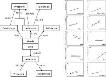
Schematic diagram of links between trophic groups and plots of a sub-set of best-fitted linear regressions of consumer on resource for June from table 2. Arrows indicate the direction of net flow of energy from resource to consumer. Figure labels show the % variation in the observed data explained from linear regressions of consumer on resource and the alpha-roman-numeric labels indicate the sub-figure in which the trophic relationship is displayed. In each case the dependent variable in the regression was chosen as the group to which energy flowed, the consumer, and the independent variable as the group from which energy flowed, the resource. The best models, shown for each relationship, were a single line, or two parallel lines, or two lines with different regression coefficients. Herbicide management was non-significant in all cases and consequently only the spring-sown oilseed rape (solid line) and winter-sown oilseed rape (dashed line) relationships are shown. The graphs are plotted only over the ranges of counts/biomass/cover observed for that relationship, with no extrapolation. The axes run, in all cases of counts and biomass, from −1⩽log(x)⩽5 along the resource axis and −1⩽log(y)⩽4 along the consumer axis. For crop cover the axes run from −1⩽log(x)⩽2 and −1⩽log(y)⩽4.

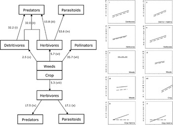
Schematic diagram of links between trophic groups and plots of a sub-set of best-fitted linear regressions of consumer on resource for year totals from table 2. Arrows indicate the direction of net flow of energy from resource to consumer. Figure labels show the % variation in the observed data explained from linear regressions of consumer on resource and the alpha-roman-numeric labels indicate the sub-figure in which the trophic relationship is displayed. In each case the dependent variable in the regression was chosen as the group to which energy flowed, the consumer, and the independent variable as the group from which energy flowed, the resource. The best models, shown for each relationship, were a single line, or two parallel lines, or two lines with different regression coefficients. Herbicide management was non-significant in all cases and consequently only the spring-sown oilseed rape (solid line) and winter-sown oilseed rape (dashed line) relationships are shown. The graphs are plotted only over the ranges of counts/biomass/cover observed for that relationship, with no extrapolation. The axes run, in all cases of counts and biomass, from −1⩽log(x)⩽5 along the resource axis and −1⩽log(y)⩽4 along the consumer axis. For crop cover the axes run from −1⩽log(x)⩽2 and −1⩽log(y)⩽4.

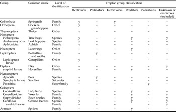
Level of identification and assigned trophic group of invertebrates from Vortis, pitfall and crop invertebrate counts.

Classification was done at the family level for Collembola, order level for Orthoptera, species level for Heteroptera, and so on; y, present in assigned functional group.
Sample data
The site selection criteria and sampling methods used for the FSEs are described in detail elsewhere (Brooks et al., Reference Brooks, Bohan, Champion, Haughton, Hawes, Heard, Clark, Dewar, Firbank, Perry, Rothery, Scott, Woiwod, Birchall, Skellern, Walker, Baker, Bell, Browne, Dewar, Fairfax, Garner, Haylock, Horne, Hulmes, Mason, Norton, Nuttall, Randle, Rossall, Sands, Singer and Walker2003; Champion et al., Reference Champion, May, Bennett, Brooks, Clark, Daniels, Firbank, Haughton, Hawes, Heard, Perry, Randle, Rossall, Rothery, Skellern, Scott, Squire and Thomas2003; Haughton et al., Reference Haughton, Champion, Hawes, Heard, Brooks, Bohan, Clark, Dewar, Firbank, Osborne, Perry, Rothery, Roy, Scott, Woiwod, Birchall, Skellern, Walker, Baker, Browne, Dewar, Garner, Haylock, Horne, Mason, Sands and Walker2003; Heard et al., Reference Heard, Hawes, Champion, Clark, Firbank, Haughton, Parish, Perry, Rothery, Scott, Skellern, Squire and Hill2003; Bohan et al., Reference Bohan, Boffey, Brooks, Clark, Dewar, Firbank, Haughton, Hawes, Heard, May, Osborne, Perry, Rothery, Roy, Scott, Squire, Woiwod and Champion2005). Briefly, plants and invertebrates were sampled from 67 SR and 65 WR fields, selected from geographic regions and conditions under which these crops are commercially grown. These fields were sampled over three growing seasons, from 2000 to 2003, with approximately one-third of the fields being sampled in each growing year (Champion et al., Reference Champion, May, Bennett, Brooks, Clark, Daniels, Firbank, Haughton, Hawes, Heard, Perry, Randle, Rossall, Rothery, Skellern, Scott, Squire and Thomas2003; Firbank et al., Reference Firbank, Perry, Squire, Bohan, Brooks, Champion, Clark, Daniels, Dewar, Haughton, Hawes, Heard, Hill, May, Osborne, Rothery, Roy, Scott and Woiwod2003b; Bohan et al., Reference Bohan, Boffey, Brooks, Clark, Dewar, Firbank, Haughton, Hawes, Heard, May, Osborne, Perry, Rothery, Roy, Scott, Squire, Woiwod and Champion2005). Each field was split, so as to minimize differences between treatments in soil type, surrounding vegetation and other potentially confounding factors, and the GMHT treatment randomly allocated to one half. Crop management of the conventional half-field was typical of current, standard commercial practice (Champion et al., Reference Champion, May, Bennett, Brooks, Clark, Daniels, Firbank, Haughton, Hawes, Heard, Perry, Randle, Rossall, Rothery, Skellern, Scott, Squire and Thomas2003; Bohan et al., Reference Bohan, Boffey, Brooks, Clark, Dewar, Firbank, Haughton, Hawes, Heard, May, Osborne, Perry, Rothery, Roy, Scott, Squire, Woiwod and Champion2005). Herbicide application to the GMHT crop followed industry recommendations and the draft product label (Champion et al., Reference Champion, May, Bennett, Brooks, Clark, Daniels, Firbank, Haughton, Hawes, Heard, Perry, Randle, Rossall, Rothery, Skellern, Scott, Squire and Thomas2003; Firbank et al., Reference Firbank, Perry, Squire, Bohan, Brooks, Champion, Clark, Daniels, Dewar, Haughton, Hawes, Heard, Hill, May, Osborne, Rothery, Roy, Scott and Woiwod2003b; Bohan et al., Reference Bohan, Boffey, Brooks, Clark, Dewar, Firbank, Haughton, Hawes, Heard, May, Osborne, Perry, Rothery, Roy, Scott, Squire, Woiwod and Champion2005). Plant and invertebrate samples were taken at up to five sample point distances into the crop along 12 transects in each half-field as described in Firbank et al. (Reference Firbank, Perry, Squire, Bohan, Brooks, Champion, Clark, Daniels, Dewar, Haughton, Hawes, Heard, Hill, May, Osborne, Rothery, Roy, Scott and Woiwod2003b).
Ground cover, mean height and vegetative and reproductive development of crop plants was recorded at six sample points per treatment on five occasions through the growing season (Champion et al., Reference Champion, May, Bennett, Brooks, Clark, Daniels, Firbank, Haughton, Hawes, Heard, Perry, Randle, Rossall, Rothery, Skellern, Scott, Squire and Thomas2003; Bohan et al., Reference Bohan, Boffey, Brooks, Clark, Dewar, Firbank, Haughton, Hawes, Heard, May, Osborne, Perry, Rothery, Roy, Scott, Squire, Woiwod and Champion2005). Weed abundance was assessed by seedling counts of each species present at all 60 sample points per treatment on three management occasions: (i) after sowing (seedling count; W1 in fig. 1); (ii) a count in May only in WR (early spring count; W2); and (iii) after herbicide applications to both treatments are complete (after herbicide count; W3). Weed abundance and biomass was also assessed during the month before harvest at 24 sample points per treatment (final count and biomass; W4 and W5) (Heard et al., Reference Heard, Hawes, Champion, Clark, Firbank, Haughton, Parish, Perry, Rothery, Scott, Skellern, Squire and Hill2003; Bohan et al., Reference Bohan, Boffey, Brooks, Clark, Dewar, Firbank, Haughton, Hawes, Heard, May, Osborne, Perry, Rothery, Roy, Scott, Squire, Woiwod and Champion2005).
Predatory and detritivorous invertebrates (mainly Carabidae, Staphylinidae, Araneae and Collembola) active at the soil surface and in the litter layer, were sampled by pitfall traps over three (P1–P3 in fig. 1) 14-day trapping periods at 12 sample points per half-field (Brooks et al., Reference Brooks, Bohan, Champion, Haughton, Hawes, Heard, Clark, Dewar, Firbank, Perry, Rothery, Scott, Woiwod, Birchall, Skellern, Walker, Baker, Bell, Browne, Dewar, Fairfax, Garner, Haylock, Horne, Hulmes, Mason, Norton, Nuttall, Randle, Rossall, Sands, Singer and Walker2003; Bohan et al., Reference Bohan, Boffey, Brooks, Clark, Dewar, Firbank, Haughton, Hawes, Heard, May, Osborne, Perry, Rothery, Roy, Scott, Squire, Woiwod and Champion2005). Phytophagous (e.g. Homoptera and Heteroptera), detritivorous (e.g. Collembola), predatory (e.g. Araneae, Carabidae and coccinellid larvae) and parasitoid insects living on the weeds and the soil surface were sampled twice (V1 and V2) with a vacuum (Vortis) suction sampler at six sample points per half-field (Haughton et al., Reference Haughton, Champion, Hawes, Heard, Brooks, Bohan, Clark, Dewar, Firbank, Osborne, Perry, Rothery, Roy, Scott, Woiwod, Birchall, Skellern, Walker, Baker, Browne, Dewar, Garner, Haylock, Horne, Mason, Sands and Walker2003; Bohan et al., Reference Bohan, Boffey, Brooks, Clark, Dewar, Firbank, Haughton, Hawes, Heard, May, Osborne, Perry, Rothery, Roy, Scott, Squire, Woiwod and Champion2005). Pollinators (bees and butterflies) were counted on four 100 m line transects into the crop on three (B1–B3) and four (B1–B4) occasions in spring and winter oilseed rape, respectively (Haughton et al., Reference Haughton, Champion, Hawes, Heard, Brooks, Bohan, Clark, Dewar, Firbank, Osborne, Perry, Rothery, Roy, Scott, Woiwod, Birchall, Skellern, Walker, Baker, Browne, Dewar, Garner, Haylock, Horne, Mason, Sands and Walker2003; Bohan et al., Reference Bohan, Boffey, Brooks, Clark, Dewar, Firbank, Haughton, Hawes, Heard, May, Osborne, Perry, Rothery, Roy, Scott, Squire, Woiwod and Champion2005). Pollinator numbers were transformed to yield a count of individuals, per km of transect walked for each sampling occasion and year total. Finally, herbivores, predators and parasitoids present on the crop were assessed twice (C1 and C2) in situ by direct observations of 45 crop plants per treatment (Hawes et al., Reference Hawes, Haughton, Osborne, Roy, Clark, Perry, Rothery, Bohan, Brooks, Champion, Dewar, Heard, Woiwod, Daniels, Young, Parish, Scott, Firbank and Squire2003).
Statistical analysis
The treatment of FSE data has been detailed elsewhere (Perry et al., Reference Perry, Rothery, Clark, Heard and Hawes2003) and is summarized briefly here. Records for each variable analysed were obtained from systematic samples within each of 2n halved-fields of each crop, in a randomized block experimental design, in which the blocks were paired halved-fields. The total count, c ij, and biomass, w ij, per half-field, for treatment i at site j, was transformed to either l ij=log (c ij+1) or l ij=log (w ij+0.005), respectively. Response variables were analysed separately for each comparison. For each particular sample point distance into the field, the half-field total for that distance was deemed missing if over half of the samples were missing. If half or fewer samples were missing, those missing samples were estimated proportionately. If the half-field total for a particular distance was regarded as missing, then so was the overall half-field total, and that site contributed no information towards the estimated treatment effect. Sites for which the whole-field total count, c 1j+c 2j, was zero or unity were removed from the analyses. To give an approximate indication of abundance, geometric means for each treatment i were calculated from backtransformed values of l ij. The standard analysis of abundance was a randomized block ANOVA of the transformed values, lij, termed the lognormal model by Perry et al. (Reference Perry, Rothery, Clark, Heard and Hawes2003). Treatment effects were tested for using a paired randomization test, using as a test statistic d=∑j[l 2j−l 1j]/n, the mean of the differences between treatments on the logarithmic scale. The treatment effect was measured as R, the multiplicative ratio of the GMHT treatment divided by the conventional, calculated as R=10d; confidence limits about R were obtained by back-transformation of the confidence interval of d on the logarithmic scale, derived from the standard error of d and t (0.05).
Simple linear regressions for logarithmically-transformed half-field totals were conducted for each of five consumer variables (predators, parasitoids, pollinators, herbivores and detritivores) on each of three resource variables (herbivores, detritivores and plants). A co-variate for the growing year that each sample was taken, between 2000 and 2003, was initially included in a full model analysis of all the sample data. In no case did the co-variate, or its interaction terms, prove statistically significant, and it was therefore excluded from all analyses. Consequently, for each combination of resource and consumer, seven regression models were compared: (i) a single line through all treatments; (ii) two parallel lines allowing the intercept to vary for each herbicide management treatment; (iii) two parallel lines allowing the intercept to vary with each crop sowing date treatment; (iv) four parallel lines allowing the intercept to vary with herbicide management and sowing date; (v) two lines allowing the intercept and regression coefficient to vary with each herbicide management treatment; (vi) two lines allowing the intercept and regression coefficient to vary with each crop sowing date treatment; and (vii) four lines allowing the intercept and regression coefficient to vary with herbicide management and sowing date. Discrimination between models was by standard partial F-tests on one degree of freedom (Sokal & Rohlf, Reference Sokal and Rohlf1981, section 14.9; Perry, Reference Perry1982). The goodness of fit of the models was scrutinized by checking the model standardized residuals for normality and evidence of systematic variation. The intercepts and regression coefficients of the best-fitting model were recorded.
Results
Tests of the null hypotheses
The null hypotheses, for effects of herbicide management and sowing date, were rejected (appendices 1 and 2). Across comparisons by year total, management occasion and calendar date, the herbivore, pollinator, detritivore, predator and parasitoid trophic groups and the dicot, monocot and total weeds groups all showed significant effects for both herbicide management and sowing date. For the dicot, monocot and total weeds groups, significant interaction effects were found in over half of the cases tested, indicating that different herbicide management effects were observed in the two crops.
For the crop itself, there was little effect of herbicide management on height or cover, but there were clear differences between spring- and winter-sown oilseed rape (appendix 1). Primary production was greatest in WR, with crop height and cover being higher at comparable calendar date and management occasions. Weed production was also greater in WR, due primarily to the greater counts and biomass of monocot weeds. Dicot numbers tended to be greater under conventional herbicide management and made up a greater proportion of total weed numbers and biomass in SR. Few interaction effects between the herbicide management and sowing date treatment effects were found.
Amongst the invertebrates, interactions between herbicide management and crop sowing date were only found for the predators of crop herbivores (appendix 2). In WR, higher numbers of these predators were found under conventional herbicide management, whereas more were found under GMHT management in SR. Weed and crop herbivores, predators, pollinators and parasitoids tended to be higher under conventional herbicide management and in SR. Only detritivore numbers were generally greater under GMHT management and in WR.
Relationships between trophic groups
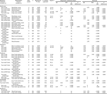
For all consumer-resource groups, significant regression relationships were observed either at the June or year total comparison (table 2, figs 2 and 3). Indeed, of the 39 analyses conducted 25, or approximately 64%, explained upwards of 5% of the variation in the observed data with an overall average of 23.3%. Herbicide management did not appear as a significant term in any analysis. In contrast, sowing date showed significant effects in 26 (66.7%) of the 39 regressions.
Functional relationships between trophic groups.

Relationships are expressed as linear regressions of resource variables on consumer variables, as defined in fig. 2, for the June and year total comparisons. Best model is either: S, a single line with common slope and intercept for both crops; P, two parallel lines with common slope but different intercepts for each crop; or D, two lines with different slope for each crop. For the regression coefficient and intercept, each crop has an associated probability value, P. When the best model is that the crops do not differ, a single probability is given for the test of whether the estimated slope or intercept differs from zero. When the best model is that the crops do differ, two probabilities are given; the first is for the test of whether the value for SR differs significantly from zero and the second indicates the level for the test of equality between the values for WR and SR. A subset of the regression relationships are displayed in fig. 3, with the fig. 3 column in this table indicating the appropriate sub-figure. SR, Spring-sown oilseed rape; WR, winter-sown oilseed rape.
At the June comparison, herbivore and pollinator trophic groups showed no response to weed counts. The pollinator intercept was higher in WR. The year totals of the herbivore and pollinator groups were positively related to final weed abundance, with a higher intercept in SR, where weed numbers were lower overall but the proportion of dicots was higher. The year total of detritivores was found to be unrelated to final weed counts, suggesting that final standing weed numbers are not useful in explaining the weed detritus needed earlier in the year to support detritivore numbers. However, for the May and June comparison dates, detritivores were greater in WR and negatively related to weed counts. Year totals of detritivores in pitfall traps produced few relationships with weeds. In general, we found that consumers of living plant material were positively related to the abundance of their resource and tended to occur at greater abundance in spring-sown oilseed rape. Conversely, consumers of dead plant material, the detritivores, were negatively related to living plant material and occurred at higher abundance in winter-sown oilseed rape.
For the June and year total comparisons, predator and parasitoid trophic groups were found to be positively related to their prey resource, whether weed herbivore, crop herbivore or detritivore (table 2). The percentage of variation explained by these relationships, as with the pollinator relationships, was high. Predators feeding on herbivores and detritivores, when summed over the year, were greater in number in SR than WR. Predator numbers were higher in WR in June. Across the year, the intercept for the combined Vortis capture of detritivores and herbivores was greater in WR, but similar in both crops in June. Although predator and parasitoid consumers were positively related to their resources, significant differences in regression coefficients were estimated for these two groups in SR and WR. In general, predators and parasitoids inhabiting SR had estimated coefficients greater than WR. This would suggest not only that the numbers of predators and parasitoids were greater in SR, but that their trophic relationships were different from that in WR.
The summed year totals for predator and parasitoid abundance were not related to crop cover or the final weed counts, although numbers of these natural enemies were higher in SR than in WR (table 2). Fitting these summed year totals for predator and parasitoid abundance as a covariate in the herbivore and primary producer relationships suggested that natural enemies were important mediators of herbivore abundance, though, explaining more variation in combination with plants than either plants or natural enemies alone (table 3). There were no significant interactions between the covariate, herbicide management and sowing date treatments, and the resource groupings. For year total crop herbivores, positive relationships were found for crop cover and natural enemy abundance, with a lower intercept in WR. Positive relationships were found for year total weed herbivore abundance and final weed counts and natural enemy abundance, with a higher intercept in WR.
Functional relationships between year total herbivore consumer trophic groups and their plant resource, with a covariate of natural enemy counts.

Best fitted model was two parallel planes, one for each crop. For the regression coefficients (slopes) each crop has a single associated probability value, P, for the test of whether the coefficient differs from zero. For the intercept, two probabilities are given; the first is for the test of whether the value for SR differs significantly from zero and the second indicates the level for the test of equality between the values for WR (winter-sown oilseed rape) and SR (spring-sown oilseed rape).
Discussion
Our analyses, based on broad trophic groups, provided a good explanation of consumer-resource relationships. Of the 41 relationships examined with linear regression models, 33 (80%) showed a significant fit and explained a considerable amount of the observed variation; particularly for pollinator, predator and parasitoid trophic groups. Using linear regression, herbicide management did not occur as a significant term in any of the relationships, whilst the composite treatment sowing date was important in 28 (68%) of the analyses. We believe that these findings lead to three general conclusions concerning the dynamics of trophic relationships: (i) herbicide management, associated with conventional and GMHT cropping, did not have a significant impact on relationships between plant and insect trophic groups; (ii) differences in sowing date between spring- and winter-sown oilseed rape were extremely important, supporting the statement of Hawes et al. (Reference Hawes, Haughton, Osborne, Roy, Clark, Perry, Rothery, Bohan, Brooks, Champion, Dewar, Heard, Woiwod, Daniels, Young, Parish, Scott, Firbank and Squire2003) that differences in abundance of trophic groups were much greater between crops than between herbicide treatments; and (iii) the herbicide management effects measured in tests of the null hypotheses here, and in previous publications (Brooks et al., Reference Brooks, Bohan, Champion, Haughton, Hawes, Heard, Clark, Dewar, Firbank, Perry, Rothery, Scott, Woiwod, Birchall, Skellern, Walker, Baker, Bell, Browne, Dewar, Fairfax, Garner, Haylock, Horne, Hulmes, Mason, Norton, Nuttall, Randle, Rossall, Sands, Singer and Walker2003; Champion et al., Reference Champion, May, Bennett, Brooks, Clark, Daniels, Firbank, Haughton, Hawes, Heard, Perry, Randle, Rossall, Rothery, Skellern, Scott, Squire and Thomas2003; Haughton et al., Reference Haughton, Champion, Hawes, Heard, Brooks, Bohan, Clark, Dewar, Firbank, Osborne, Perry, Rothery, Roy, Scott, Woiwod, Birchall, Skellern, Walker, Baker, Browne, Dewar, Garner, Haylock, Horne, Mason, Sands and Walker2003; Heard et al., Reference Heard, Hawes, Champion, Clark, Firbank, Haughton, Parish, Perry, Rothery, Scott, Skellern, Squire and Hill2003; Roy et al., Reference Roy, Bohan, Haughton, Hill, Osborne, Clark, Perry, Rothery, Scott, Brooks, Champion, Hawes, Heard and Firbank2003; Bohan et al., Reference Bohan, Boffey, Brooks, Clark, Dewar, Firbank, Haughton, Hawes, Heard, May, Osborne, Perry, Rothery, Roy, Scott, Squire, Woiwod and Champion2005), should be explicable using trophic relationships that have no explicit herbicide management terms.
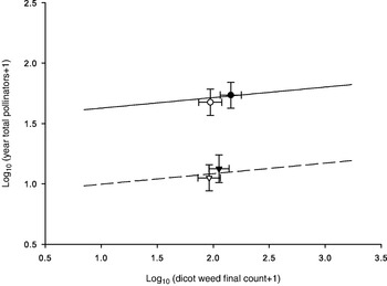
In tests of the null hypothesis, it was clear that detritivore numbers were greater under GMHT management, whilst most other trophic groups occurred at highest abundance under conventional herbicide management. These findings are explicable from the fitted regression relationships between resource and consumer groups. Using the year total pollinators as an example (fig. 4), numbers were positively related to dicots, with no effect of herbicide management. However, in both crops, dicot numbers were higher under conventional herbicide management regimes, leading to greater abundance of pollinators in conventional compared to GMHT management found in the tests of the null hypotheses. There is, therefore, nothing unique about the dynamics of GMHT herbicide management. Conventional and GMHT herbicide management regimes tend to lie at different points along the same consumer-resource relationship within each crop.
Plot of mean (and 95% confidence intervals) for conventional (closed symbols) and genetically modified, herbicide-tolerant GMHT (open symbols) herbicide management in spring-sown (circle symbols) and winter-sown (triangle symbols) oilseed rape. The lines represent the two parallel lines model, best fitted using linear regression to the spring-sown oilseed rape (solid line) and winter-sown oilseed rape (dashed line), for year total pollinators on final count dicots (also represented as fig. 3 (vii)). The year total pollinators were found to be positively related to dicots. In both spring- and winter-sown oilseed rape, dicot numbers were higher under conventional herbicide management regimes, leading to greater abundance of pollinators in conventional, compared to GMHT, management found in the null hypothesis testing. Means for the conventional and GMHT herbicide management regimes, therefore, tend to lie at different points along the same consumer-resource relationship within each crop.

The apparent lack of importance of the herbicide management regimes on the trophic relationships observed in oilseed rape contrasts with the finding of Hawes et al. (Reference Hawes, Haughton, Osborne, Roy, Clark, Perry, Rothery, Bohan, Brooks, Champion, Dewar, Heard, Woiwod, Daniels, Young, Parish, Scott, Firbank and Squire2003) that GMHT relationships were significantly different from those under conventional herbicide management in spring-sown beet and maize. This contrast may be a product of the strength of the relationship between weed herbivores and their weed resource. Hawes et al. (Reference Hawes, Haughton, Osborne, Roy, Clark, Perry, Rothery, Bohan, Brooks, Champion, Dewar, Heard, Woiwod, Daniels, Young, Parish, Scott, Firbank and Squire2003) found no relationship between weeds and herbivore numbers in SR, and here the year total relationship for WR was relatively weak, explaining only 5.7% of the observed variation in herbivore numbers. This low variation explained may mean that herbicide management and weed abundance has little effect upon weed herbivore numbers and, consequently, on the abundance of invertebrates that are trophically related to the herbivores. Bohan et al. (Reference Bohan, Boffey, Brooks, Clark, Dewar, Firbank, Haughton, Hawes, Heard, May, Osborne, Perry, Rothery, Roy, Scott, Squire, Woiwod and Champion2005) suggested for WR, that the large bulky crop might buffer any effect of weed abundance. The results might also suggest that the basic assumption used for the FSEs (Firbank et al., Reference Firbank, Heard, Woiwod, Hawes, Haughton, Champion, Scott, Hill, Dewar, Squire, May, Brooks, Bohan, Daniels, Osborne, Roy, Black, Rothery and Perry2003a), namely that weed dynamics drive the dynamics of the invertebrates, might not be appropriate for oilseed rape.
Koricheva et al. (Reference Koricheva, Mulder, Schmid, Joshi and Huss-Danell2000) and Siemann et al. (Reference Siemann, Tilman, Haarstad and Ritchie1998) found that herbivore abundance in grassland systems was more dependent upon natural enemy numbers than the availability of primary producer foodstuffs, which were present in excess. Here we found that the summed numbers of predators and parasitoids in SR and WR were not related either to crop cover or final weed counts, but that significantly more variation in herbivore numbers could be explained by the inclusion of the summed parasitoid and predator abundance as a covariate in the herbivore-primary producer regressions than either variate alone. Such findings support the conclusions of Koricheva et al. (Reference Koricheva, Mulder, Schmid, Joshi and Huss-Danell2000) and Siemann et al. (Reference Siemann, Tilman, Haarstad and Ritchie1998) and suggest that predation and parasitism by natural enemies may obscure the relationship between herbivore consumers and primary producer resources in oilseed rape. Thus, the validity of the assumption that primary production drives the dynamics of invertebrates may be crop-dependent and needs to take account of likely differences in the importance of natural enemies.
The agronomic and varietal package of effects rolled up in to the sowing date treatment exerted an important effect on the dynamics of trophic relationships. In general, over most resource ranges, numbers of consumers in SR crops were greater than in WR. The year totals results should be treated with some caution, however. WR year totals could include data from a sampling point in the autumn when, in comparison to the equivalent management occasion in SR in the spring, in-field invertebrate numbers may be low prior to overwintering (Bohan et al., Reference Bohan, Boffey, Brooks, Clark, Dewar, Firbank, Haughton, Hawes, Heard, May, Osborne, Perry, Rothery, Roy, Scott, Squire, Woiwod and Champion2005). For analysis, the intercept in WR might, therefore, be expected to be lower than that in SR, as was found. However, this does not explain the results for detritivores which were greater under WR, pollinators which were higher in SR at comparable calendar and management occasions, and parasitoid and predator groups that had higher regression coefficients in SR than WR. Whilst recognising that some care should be taken in interpretation, we believe that SR does indeed have a greater non-detritivore invertebrate abundance than WR since WR cropping promotes a trophic pathway based upon dead weeds and detritivores whilst SR promotes living weeds and a trophic pathway based upon herbivores.
These findings would appear not to change with the year of observation. In contrast to the expectation that year to year variation in weather and longer term impacts may affect the observed numbers in any one growing season (see for example Aebischer, Reference Aebischer, Firbank, Carter, Derbyshire and Potts1991), a co-variate for the growing season was never significant and was consequently removed from the analysis. This finding is consistent with that for the baseline papers of the FSEs, where no more ‘year effects’ were significant than expected by chance. It was believed that this was because ‘as the number of sites is increased, particularly when they are widely distributed over a large geographical area, treatment×year interactions are minimized’ (Brooks et al., Reference Brooks, Bohan, Champion, Haughton, Hawes, Heard, Clark, Dewar, Firbank, Perry, Rothery, Scott, Woiwod, Birchall, Skellern, Walker, Baker, Bell, Browne, Dewar, Fairfax, Garner, Haylock, Horne, Hulmes, Mason, Norton, Nuttall, Randle, Rossall, Sands, Singer and Walker2003).
The observed shift between trophic pathways would help explain why there tended to be higher counts of particular trophic groups in SR or WR, under the tests of the null hypotheses, but it does not alone explain why the sowing date treatment gave different regression relationships, with different intercepts and/or regression coefficients. Such changes in relationship would imply that the efficiency of conversion of resource (energy) into consumer trophic groups is modified with sowing date. The parasitoid and predator trophic groups, which tend to have higher regression coefficients in SR than WR, share a number of important properties that could provide clues to this change in efficiency. In general, invertebrate parasitoids and predators reside within the field and actively search for multiple prey resource items. Under laboratory conditions, a reduction in regression coefficient value between prey resource and these consumer trophic groups would typically be interpreted as a reduction in consumer searching efficiency or resource apparency (Godfray, Reference Godfray1994). This interpretation is congruent to the field situation we describe. WR is a much more bulky crop than SR with greater cover and height. This bulk could mean that parasitoid and predator searching would be much less efficient in WR leading to lower regression coefficient estimates. Weed apparency might also explain differences in intercepts for the pollinators, although this pollinator effect may mainly be explained by the SR crop being in flower during the July sampling period and contributing disproportionately to the year total counts (appendix 2). Interestingly, in SR where there were more predator and parasitoid natural enemies, we found fewer weed herbivores per natural enemy, compared to WR, and correspondingly fewer herbivores per weed plant. If this lower ratio of herbivores to natural enemies and herbivores to weeds in SR was due to differences in apparency between the two crops, then we would argue that the natural enemies were significantly reducing herbivore numbers; a possible combination of total herbivore numbers being limited, bottom-up, by weed abundance (Root, Reference Root1973; Cromartie, Reference Cromartie1975; Fretwell, Reference Fretwell1977, Reference Fretwell1987; Price et al., Reference Price, Bouton, Gross, McPheron, Thompson and Weis1980; Oksanen et al., Reference Oksanen, Fretwell, Arruda and Niemela1981; Stinson & Brown, Reference Stinson and Brown1983) and regulated, top-down, by natural enemies (Carpenter et al., Reference Carpenter, Kitchell and Hodgson1985; McNaughton, Reference McNaughton1985; McQueen et al., Reference McQueen, Post and Mills1986, Reference McNaughton, Oesterheld, Frank and Williams1989; Carpenter & Kitchell, Reference Carpenter and Kitchell1988; McNaughton et al., Reference McNaughton, Oesterheld, Frank and Williams1989; Hunter & Price, Reference Hunter and Price1992; Power, Reference Power1992; Osenberg & Mittelbach, Reference Osenberg, Mittelbach, Polis and Winemiller1996). Such a combination of bottom-up limitation and top-down regulation would certainly explain the relatively low percentage of variation in weed herbivore abundance accounted for by weed data alone and could also indicate why few invertebrates were found to respond to the herbicide management, particularly in WR (Bohan et al., Reference Bohan, Boffey, Brooks, Clark, Dewar, Firbank, Haughton, Hawes, Heard, May, Osborne, Perry, Rothery, Roy, Scott, Squire, Woiwod and Champion2005).
This line of reasoning would suggest that differences in crop structure and resource apparency, associated with the sowing date treatment, may explain differences in the links between trophic groups in SR and WR, more so than an actual difference in the date of sowing itself. Whatever the correct explanation, the change in slope for the predators and parasitoids between SR and WR has some interesting ecological implications. The lower efficiency of resource conversion into consumers, in WR, could indicate that where a shift from SR- to WR-dominated landscapes has occurred, these groups might ‘jump’ from one trophic relationship to the other, moving between different stable states (Hassell et al., Reference Hassell, Southwood and Reader1987). In essence, with a move to WR, parasitoid and predator dynamics could have entered a different envelope of abundance dynamics.
The resource-consumer regression relationships fitted here explain a large proportion of the variation within all groups (an approximate mean of 23%), suggesting that broad trophic groups and the cascade of relationships between them might provide a basis for constructing straightforward, pragmatic models for the dynamics of invertebrates in farmland. Using the linear regression, for parameterization, and the schematic structure in fig. 2, trophically-based models could be expected to have a common structure, yet would be able to describe dynamics across distinct management classes. Accuracy might be improved by finer subdivision of invertebrates based, for example, on phenology, activity patterns (nocturnal vs. diurnal, etc.) or degree of ecological specialization. Clearly, though, there is a need for a parsimonious solution, trading-off simplification into, and the possible generality of, broad trophic groups with complex definitions where groups are effectively synonyms for species that might also not explain significantly more of the variation in the data.
Acknowledgements
The authors would like to thank the members of the consortium of scientists who conducted the Farmscale Evaluations of GMHT crops. We would also like to thank Juliet Osborne, John Pidgeon and Robin Thompson for constructive comments on the manuscript. This work was funded by Defra and the Scottish Executive. Rothamsted Research receives grant-aided support from the BBSRC.
Appendix 1
Vegetation analyses for the weeds (A) and crop (B). Mean primary producer group abundance (m−2), biomass (gm−2), cover (%) and height (cm) with herbicide management and sowing date management classes. Comparisons are made between samples taken on comparable calendar dates, management occasions and crop growth stages.


Appendix 2
Geometric mean invertebrate trophic group abundance with herbicide management and sowing date management classes. Comparisons are made between samples taken at comparable calendar dates and between year totals.