




1. Introduction
We consider the following stochastic differential equation (SDE) with
 $X_0=x_0\in\mathbb{R}^d$
fixed:
 \begin{equation}{\mathrm{d}} X_t = a\big(X_t,\overline{\xi}_1(X_t,\mu_t)\big)\,{\mathrm{d}} t + b\big(X_t,\overline{\xi}_2(X_t,\mu_t)\big)\,{\mathrm{d}} W_t,\end{equation}
where, for
 $j\in\{1,2\}$
,
 $\overline{\xi}_j(X_t,\mu_t) = \int_{\mathbb{R}^d}\xi_j(X_t,x)\,\mu_t({\mathrm{d}} x)$
,
 $\{W_t\}_{t\geq 0}$
is a standard d-dimensional Brownian motion,
 $\mu_t$
is the law of
 $X_t$
,
 $a\colon\mathbb{R}^d\times\mathbb{R}\rightarrow\mathbb{R}^d$
,
 $b\colon\mathbb{R}^d\times\mathbb{R}\rightarrow\mathbb{R}^{d\times d}$
, and
 $\xi_j\colon\mathbb{R}^{2d}\rightarrow\mathbb{R}$
. In this paper we assume that the functions
 $\xi_j$
are convolution-type functions, that is
 $\xi_j(x,y) = \zeta_j(x-y)$
for a function
 $\zeta_j\colon\mathbb{R}^d\rightarrow\mathbb{R}$
. This restriction on
 $\xi_j$
is discussed below. McKean–Vlasov SDEs such as (1) have a wide variety of real applications such as in biology and finance [Reference Bush, Hambly, Haworth, Jin and Reisinger5, Reference Dobramysl, Rudiger and Erban12]; in addition, they have been shown to be an equivalent representation of solutions of classes of nonlinear partial differential equations [Reference Barbu and Roeckner2], and even more applications can be expected in the future. The exact problem addressed in this article is where the process defined in (1) is only observed with noise at regular and discrete times. The objective is then to compute the conditional expectation of
 $X_t$
(or functionals thereof) given all the observations recursively at every observation time, which is a filtering problem; see, e.g., [Reference Bain and Crisan1, Reference Cappé, Ryden and Moulines6] for an introduction.
The filtering of continuous-time processes is very challenging. First, even if the transition densities of the process exist and are analytically tractable, filtering must normally be performed by using numerical methods, of which we focus on particle filters (PFs); see, e.g., [Reference Bain and Crisan1, Reference Cappé, Ryden and Moulines6, Reference Del Moral9]. Second, the aforementioned transition densities are seldom available and hence we normally have to resort to time discretization of the process; see, for instance, [Reference Jasra, Kamatani, Law and Zhou19]. In the case of regular diffusions (i.e. where the coefficients do not depend on
 $\mu_t$
), there is already a substantial literature on using PFs for solving the filtering problem; see, e.g., [Reference Del Moral, Jacod and Protter10, Reference Fearnhead, Papaspiliopoulos and Roberts14]. In addition to these methods, PFs have been extended to leverage the popular multilevel Monte Carlo (MLMC) method [Reference Giles15, Reference Giles16, Reference Heinrich18]. These multilevel PFs (MLPFs) [Reference Jasra, Kamatani, Law and Zhou19, Reference Jasra, Kamatani, Osei and Zhou20, Reference Jasra, Maama and Ombao23] can reduce the cost to compute the filtering expectation for a given mean square error (MSE).
To the best of our knowledge, there are few articles in the context of numerical methods for filtering McKean–Vlasov SDEs, particularly when using multilevel Monte Carlo. There are several interesting works on the theory of such models in [Reference Qiao and Wei28, Reference Sen and Caines29]. In addition, there are articles that consider using a McKean–Vlasov representation for filtering, such as [Reference Crisan and Xiong8], but these methods are not designed for our filtering problem, nor do they necessarily use any multilevel methods. However, when trying to compute expectations with respect to the laws of such processes, several methods have been proposed. This includes the initial work of [Reference Sznitman30] that relies on time discretization and simulation coupled with solving backward Kolmogorov equations; this can be prohibitive if d is even moderate. Several recent extensions based on using the aforementioned simulation and designing change of measures for importance sampling have been considered in [Reference Dos Reis, Smith and Tankov13] and then combined with MLMC [Reference Ben Rached, Haji-Ali, Shyam and Tempone4] or multi-index MC (see [Reference Haji-Ali, Nobile and Tempone17]) [Reference Ben Rached, Haji-Ali, Shyam and Tempone3]. An iterative method combined with MLMC was also proposed in [Reference Szpruch, Tan and Tse31]. Despite these high-quality and interesting contributions, none of these methods are designed for the filtering problem and would likely have several deficiencies. For instance, if the change of measure methods were adopted, it is likely that they would suffer from the well-known weight-degeneracy problem (e.g. [Reference Cappé, Ryden and Moulines6, Reference Del Moral9]). That is, the estimates of the filter would suffer an exponential increase of variance with respect to observation times. The approach of [Reference Szpruch, Tan and Tse31] is iterative and thus is not appropriate for the filtering problem as we seek fast (non-iterative) methods to assimilate the data.
In this paper we develop new PF and MLPF methodologies to estimate the filter associated with partially observed McKean–Vlasov SDEs recursively in time. This requires some care as, unlike the case of filtering ordinary diffusions, even under a time discretization we cannot simulate the MVSDE. This is because the law of the discretized process is not known and must be estimated. We show how the idea adopted in [Reference Ben Rached, Haji-Ali, Shyam and Tempone4, Reference Dos Reis, Smith and Tankov13] can be leveraged. That is, to use the particle system of [Reference Sznitman30] to be fed into a ‘classical’ PF; this resulting algorithm can be used to recursively estimate the filter. We then show how this idea can be extended to the multilevel context by combining with ideas from [Reference Jasra, Kamatani, Law and Zhou19, Reference Jasra, Yu and Heng26]; see [Reference Jasra, Law and Suciu21] for a review and [Reference Jasra, Law and Yu22] for related methodology. We prove, under assumptions, that for
 $\varepsilon>0$
to achieve an MSE associated with estimating the filter of
 $\mathcal{O}(\varepsilon^2)$
per observation time,
-
• the cost for the PF is
 $\mathcal{O}(\varepsilon^{-5})$
;
-
• the cost for the MLPF is
$\mathcal{O}(\varepsilon^{-4})$
(best case) or
$\mathcal{O}(\varepsilon^{-4}\log(\varepsilon)^2)$
(worst case).



The best case corresponds to the case where the diffusion coefficient b in (1) is constant and the other case is for non-constant b – of course, only when the MVSDE follows our assumptions. The costs above are higher than we might expect for ordinary Monte Carlo-based methods (which PFs and MLPFs are). These increased costs are primarily associated with having to approximate the laws
 $\mu_t$
(and their time-discretized versions) in the evolution of the MVSDE. It may be possible to reduce the costs by using multi-index Monte Carlo [Reference Haji-Ali, Nobile and Tempone17] as was adopted in [Reference Ben Rached, Haji-Ali, Shyam and Tempone3], but this is not investigated in this paper. The MSE-to-cost results are verified in several numerical examples.
The proposed methodologies presented in this paper are general and do not require the convolution-type assumption on
 $\xi_j$
for their implementation. The assumption is required to provide bounds on the error of the methods, specifically the bias of the proposed methods, which requires the stringent conditions of infinite smoothness and convolution type
 $\xi_j$
. The rate of the bias is not well known for the general case of McKean–Vlasov SDEs. The variance, on the other hand, does not require infinite smoothness or the convolution-type assumption. For this reason we keep the notation
 $\xi_j$
and introduce Assumption (W2) below.
This article is structured as follows. In Section 2 we give our approach to filtering partially observed McKean–Vlasov SDEs. In Section 3, our theoretical results are presented. Section 4 details our numerical results associated with the methodology. Our proofs can be found in the appendix.
2. Approach
2.1. State-space model
We denote by
 $P_{\mu_{t-1},t}(x_{t-1},{\mathrm{d}} x_t)$
the conditional law of
 $X_t$
(as given in (1)) given
 $\mathscr{F}_{t-1}$
(the natural filtration of the process) for
 $t\geq 1$
; that is, the transition kernel over unit time. We consider a discrete-time observation process
 $Y_1,Y_2,\dots,Y_t\in\mathsf{Y}$
, assumed, for notational convenience, to be observed at unit times. Conditional on the position
 $X_t$
,
 $t\in\mathbb{N}$
, of (1), the random variable
 $Y_t$
is assumed to be independent of all other random variables, with a bounded and positive probability density
 $G(x_t,y_t)$
. We note that
 $G(x_t,y_t)$
for each
 $t\geq 1$
must be a tractable probability density, that is, it exists and can be evaluated pointwise. This is a requirement of the approach that we are going to detail. If this is not the case there are some solutions using approximate Bayesian computation; see [Reference Jasra, Singh, Martin and McCoy24], for example.
Let
 $\varphi\colon\mathbb{R}^d\rightarrow\mathbb{R}$
be a bounded and measurable function (write a collection of such functions as
 $\mathcal{B}_\mathrm{b}(\mathbb{R}^d)$
), then we define the filtering expectation for
 $t\in\mathbb{N}$
as
 \begin{align*}\pi_t(\varphi) \,:\!=\,\frac{\int_{\mathbb{R}^{dt}}\varphi(x_t)\big\{\!\prod_{p=1}^tG(x_p,y_p)\big\}\prod_{p=1}^tP_{\mu_{p-1},p}(x_{p-1},{\mathrm{d}} x_p)}{\int_{\mathbb{R}^{dt}}\big\{\!\prod_{p=1}^tG(x_p,y_p)\big\}\prod_{p=1}^tP_{\mu_{p-1},p}(x_{p-1},{\mathrm{d}} x_p)},\end{align*}
where
 $\mu_0=\delta_{\{x_0\}}$
(the Dirac measure on the set
 $\{x_0\}$
). We remark that we do not need
 $\varphi$
or each of the
 $G(\cdot,y_t)$
to be bounded, but it will simplify the resulting exposition to do so.
In most cases of practical interest,
 $\mu_t$
and the dynamics
 $P_{\mu_{t-1},t}(x_{t-1},{\mathrm{d}} x_t)$
are difficult to work with. For instance, the transition kernel cannot be simulated in many problems. As a first step to approximating the filter
 $\pi_t$
, we introduce a time discretization over a regular grid of spacing
 $\Delta_l=2^{-l}$
,
 $l\in\mathbb{N}_0$
. The significance of the subscript l is that it will denote the level of discretization – as l grows, so will the accuracy of the time discretization. We will use the Euler–Maruyama method associated with (1) and denote the law at any time
 $t\in\{0,\Delta_l,2\Delta_l,\dots\}$
as
 $\mu_t^l$
. That is, we now consider the approximation, for
 $k\in\mathbb{N}_0$
,
 \begin{align} X_{k\Delta_l} & = X_{(k-1)\Delta_l} + a\big(X_{(k-1)\Delta_l},\overline{\xi}_1(X_{(k-1)\Delta_l},\mu_{(k-1)\Delta_l}^l)\big)\Delta_l \nonumber \\[5pt] & \quad + b\big(X_{(k-1)\Delta_l},\overline{\xi}_2\big(X_{(k-1)\Delta_l},\mu_{(k-1)\Delta_l}^l\big)\big) [W_{k\Delta_l} - W_{(k-1)\Delta_l}], \end{align}
where
 $X_0=x_0$
and
 $\mu_0^l=\delta_{\{x_0\}}$
. Associated with (2), we denote by
 $P_{\mu_{t-1},t}^l(x_{t-1},{\mathrm{d}} x_t)$
the conditional law of
 $X_t$
,
 $t\in\mathbb{N}$
, given
 $\mathscr{F}_{t-1}$
for
 $t\geq 1$
; that is, the transition kernel over unit time induced by (2). It should be remarked that in many cases (2) cannot be simulated exactly as the expectations associated with
 $\mu_{k\Delta_l}^l$
cannot be computed even if we know
 $\mu_{(k-1)\Delta_l}^l$
, which is again unlikely.
Our objective now is to compute an approximation of the time-discretized filtering expectation for
 $(t,l,\varphi)\in\mathbb{N}\times\mathbb{N}_0\times\mathcal{B}_\mathrm{b}(\mathbb{R}^d)$
:
 \begin{align*}\pi_t^l(\varphi) \,:\!=\,\frac{\int_{\mathbb{R}^{dt}}\varphi(x_t)\big\{\!\prod_{p=1}^tG(x_p,y_p)\big\}\prod_{p=1}^tP_{\mu_{p-1}^l,p}^l(x_{p-1},{\mathrm{d}} x_p)}{\int_{\mathbb{R}^{dt}}\big\{\!\prod_{p=1}^tG(x_p,y_p)\big\}\prod_{p=1}^tP_{\mu_{p-1}^l,p}^l(x_{p-1},{\mathrm{d}} x_p)}.\end{align*}
In the above formulation
 $X_0$
is taken as fixed. In terms of the methodology to be discussed, there is no issue in allowing it to be random, and we remark in Section 2.5 on what modifications would have to be made. This is also the case with regards to the mathematical results that we will present. As our numerical implementations take
 $X_0$
as fixed and this also makes the presentation of the paper more compact, we have not added any stochasticity to
 $X_0$
.
2.2. Approximating the law
We now consider a method that will be used to provide a Monte Carlo-based approximation of the law
 $\mu_t^l$
. The approach we present is a simple discretized method in Algorithm 1 from [Reference Sznitman30]. In Algorithm 1, the notation
 $\mathcal{N}_d(\kappa,\Sigma)$
denotes the d-dimensional Gaussian distribution with mean
 $\kappa$
and covariance matrix
 $\Sigma$
.
 $I_d$
is the
 $d\times d$
identity matrix and
 $\stackrel{\textrm{ind}}{\sim}$
denotes ‘independently distributed as’.
Algorithm 1 can be used to approximate expectations with respect to
 $\mu_t^l$
, and indeed on the grid in-between time
 $t-1$
and t. Algorithm 1 is given in the form that we need it later on in the article. We remark that in all the applications of Algorithm 1, we will use it with
 $M\in\mathbb{N}$
or
 $M_l\in\mathbb{N}$
samples (the N in Algorithm 1. The convergence of the algorithm is as M grows and so the accuracy of our methodology, in terms of the approximation of the laws, will be in terms of M (or
 $M_l$
) and some additional particles which are now to be described. This convention is also used in the related Algorithm 3, described later.
2.3. Particle filter
An approach for the recursive approximation of
 $\pi_t^l(\varphi)$
is presented in Algorithm 2 and is run to a terminal time T – this need not be the case. This is run with
 $N\in\mathbb{N}$
particles and these are used to approximate the discretized filter
 $\pi_t^l(\varphi)$
. The convergence of this and our multilevel particle filter (described in Algorithm 5) will then be decomposed into convergence of the filter (i.e. N, or
 $N_l$
for the MLPF) and the convergence of the laws (i.e. M or
 $M_l$
). At this stage, several remarks are of interest:
-
1. The cost of Algorithm 2 is
$\mathcal{O}(\Delta_l^{-1}M(M+N))$
per observation time (or time step). -
2. In step (ii), it is critical that this process be independent of the particles that are generated in the particle filter. The empirical laws produced here are generated independently of anything that is done later on. If we use the empirical laws that were produced by the samples from the particle filter, then the approximation would be biased even if
$N,M\rightarrow\infty$
and
$l\rightarrow\infty$
. This is because these particles used in the particle filter have been designed to approximate expectations with respect to
$\pi_t$
and not the law of the McKean–Vlasov SDE itself. Thus, here the motivation of a driving approximation of the SDE marginal law, as was the case in [Reference Ben Rached, Haji-Ali, Shyam and Tempone4, Reference Dos Reis, Smith and Tankov13], is one of necessity. -
3. The variance with respect to the time parameter should be controlled and can be uniform in time. This may not be the case for the methods in [Reference Ben Rached, Haji-Ali, Shyam and Tempone4].
-
4. Improved discretization methods can be used, when available.
-
5. We will prove, later on, that as
$N,M\rightarrow\infty$
we have
$\pi_{t}^{l,N,M}(\varphi)\rightarrow_{\mathbb{P}}\pi_{t}^{l}(\varphi)$
, where
$\rightarrow_{\mathbb{P}}$
denotes convergence in probability and
$\varphi$
is in a particular class of real-valued functions to be stated.






Approximating the laws when starting with a particle approximation at time
 $t-1$
,
 $t\in\{1,\dots,T\}$

Algorithm 1 Long description
Panel A: The algorithm starts with input parameters including the level of discretization, the number of particles, and the time step. It initializes the empirical measure and sets the initial value of k. Panel B: For each particle, it generates new states using a stochastic differential equation. The equation includes terms for drift, diffusion, and random noise. The algorithm updates the empirical measure and increments k. Panel C: The process repeats until k reaches a specified value, at which point the algorithm outputs the required laws.
Particle filter for approximating
 $\pi_{t}^l(\varphi)$
for all times
 $t\in\{1,\ldots,T\}$

Algorithm 2 Long description
An equation describing a particle filter algorithm. The equation starts with the input parameters: the level of discretization, the number of particles, the number of particles for computing process laws, the final time, and initial values. The algorithm runs with these parameters and updates particle positions based on previous positions and random variables. It computes weights for each particle and samples new particles based on these weights. This process repeats until the final time is reached, at which point the estimators are returned.
Approximating the consecutive laws when starting with a particle approximation at time
 $t-1$
,
 $t\in\{1,\dots,T\}$

Algorithm 3 Long description
An equation describing the process of generating particle positions at time t-1+k*Delta_l for i ranging from 1 to N. The equation involves generating x_t-1+k*Delta_l^i based on previous positions x_t-1+(k-1)*Delta_l^i, coefficients a and b, functions xi_1 and xi_2, empirical measures mu_t-1+(k-1)*Delta_l^N, and increments of Brownian motion. The process involves setting k to 1, generating positions, and updating k until it reaches Delta_l^-1 + 1. The algorithm then computes positions at time t+k*Delta_l^-1 and updates k until it reaches Delta_l^-1 + 1. Finally, the algorithm outputs the required laws.
2.4. Multilevel particle filter
We now show how the PF can be extended into the MLMC framework, along the lines of the work in [Reference Jasra, Kamatani, Law and Zhou19]. The purpose of this is to reduce the computing cost in terms of an MSE, which is defined in Section 3. The basic idea is to approximate the identity for
 $(L,t,\varphi)\in\mathbb{N}^2\times\mathcal{B}_\mathrm{b}(\mathbb{R}^d)$
:
 $\pi_t^{L}(\varphi) = \pi_t^0(\varphi) + \sum_{l=1}^L\{\pi_t^l(\varphi)-\pi_t^{l-1}(\varphi)\}$
. The terms on the right-hand side of this equation are then approximated as follows.
 $\pi_t^0(\varphi)$
can be dealt with using the PF of Algorithm 2. Then, independently of using the PF and for each summand, we run what is called a coupled PF (CPF). This is a type of PF that allows us to approximate
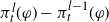 $\pi_t^l(\varphi)-\pi_t^{l-1}(\varphi)$
by producing a coupling of the sampling step (Algorithm 2, step (iii)) and a coupling of the resampling step (Algorithm 2, step (iv)). In Algorithm 2 we also use Algorithm 1, which needs to be coupled as well. This coupling, and also for the sampling step of a PF, is achieved using the well-known synchronous coupling for diffusions (and the associated Euler approximation) and is given in our coupling of Algorithm 1, which can be found in Algorithm 3. The coupling of the resampling step relies on simulating a maximal coupling and is given in Algorithm 4. As noted in [Reference Jasra and Yu25], there is nothing optimal about using this approach in a CPF, but it is rather popular in the literature and is of linear complexity in terms of the cardinality of the state space.
Given all the ideas already stated, we are now in a position to give the CPF algorithm, Algorithm 5. The cost of the CPF is
 $\mathcal{O}(\Delta_l^{-1}M(M+N))$
per observation time. We can also describe the MLPF method that we will use for the approximation of
 $\pi_t^{L}(\varphi)$
. We assume that we have
 $L\in\mathbb{N}$
given and, for each level l, the number of samples
 $N_l$
used at each level of the application of Algorithm 5, with the number of samples used for the call of Algorithm 3 within Algorithm 5 also equal to
 $M_l$
; we describe how to choose these numbers later on. Then, the procedure would be as follows:
-
1. Run Algorithm 2 with
$N_0$
samples and
$M_0$
samples for each call of Algorithm 1. -
2. Independently for each
$l\in\{1,\dots,L\}$
, run Algorithm 5 with
$N_l$
samples and
$M_l$
samples for each call of Algorithm 3.


Then our MLPF estimator of
 $\pi_t^L(\varphi)$
is. for
 $(L,t,\varphi)\in\mathbb{N}\times\mathbb{N}\times\mathcal{B}_\mathrm{b}(\mathbb{R}^d)$
,
 \begin{align*}\widehat{\pi_t^L(\varphi)} = \pi_t^{0,N_0,M_0}(\varphi) +\sum_{l=1}^L\big\{\pi_{t}^{l,N_l,M_l}(\varphi) - \pi_{t}^{l-1,N_l,M_l}(\varphi)\big\},\end{align*}
where
 $\pi_t^{0,N_0,M_0}(\varphi)$
has been computed using Algorithm 2, and each of the
 $\big(\pi_{t}^{l,N_l,M_l}(\varphi) - \pi_{t}^{l-1,N_l,M_l}(\varphi)\big)$
is produced by using Algorithm 5. The cost of computing this estimator, per time step, is
 $\mathcal{O}\big(\sum_{l=0}^L\Delta_{l}^{-1}M_l(M_l+N_l)\big)$
. In the next section we establish how to choose L,
 $(N_0,M_0),\dots,(N_L,M_L)$
so as to obtain a particular MSE and minimize the cost.
Simulating a maximal coupling

Algorithm 4 Long description
The image displays an algorithm for simulating a maximal coupling. It outlines the steps to input the cardinality of the state space and two probability mass functions. The algorithm involves sampling a uniform distribution and then sampling indices based on specific probability mass functions. The steps are detailed with mathematical expressions and conditions to follow. The final step returns the indices.
Coupled particle filter for approximating
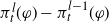 $\pi_{t}^l(\varphi)-\pi_{t}^{l-1}(\varphi)$

Algorithm 5 Long description
Panel A: The diagram begins with inputs including the level of discretization, number of particles, number of particles to compute the laws of the process, final time, and initial conditions. Panel B: It describes running Algorithm 3 at a specific time with given particles and discretization level, using the input empirical measure from the last call of Algorithm 3 if required. Panel C: For each particle and time step, it generates new states using a combination of previous states, laws of the process, and Brownian motion increments. Panel D: It computes weights for the particles based on the generated states and observations. Panel E: The algorithm updates the estimators and checks if the final time is reached, either continuing to the next time step or returning the estimators.
2.5. Random
$X_0$

We now comment on what would change in Algorithms 1, 2, 3, and 5 if
 $X_0$
is allowed to be random with distribution
 $\mu_0$
. We make the assumption that the distribution of
 $X_0$
can be sampled. In Algorithm 1, we would simply modify step (i) if
 $t=1$
by sampling N points from
 $\mu_0$
and using the N-empirical measure of these points for
 $\mu_0^N$
instead of a Dirac mass on the deterministic point
 $x_0$
. In Algorithm 2, we would change step (i) to sample N points from
 $\mu_0$
and have
 $X_0^i$
correspond to those sampled points. In Algorithm 3, there is a change to step (i) and we would again sample N points from
 $\mu_0$
and let
 $\mu_0^{l,N}=\widetilde{\mu}_{0}^{l-1,N}$
be the N-empirical measure of these points. Finally, in Algorithm 5 we would again change step (i) to sample N points from
 $\mu_0$
and have
 $X_0^{l,i}=X_0^{l-1,i}$
be these N sampled variables.
3. Theoretical analysis
3.1. Notation
Define the sets
 $\mathbb{N}=\{1,\dots\}$
and
 $\mathbb{N}_0=\{0,1,\dots\}$
. Denote by
 $\mathcal{B}_\mathrm{b}(\mathbb{R}^{d_1},\mathbb{R}^{d_2})$
the set of all
 $\mathbb{R}^{d_2}$
-valued bounded Borel measurable functions defined on
 $\mathbb{R}^{d_1}$
. For
 $k\in\mathbb{N}$
, denote by
 $\mathcal{C}^k_\mathrm{b}(\mathbb{R}^{d_1},\mathbb{R}^{d_2})$
the set of k-times continuously differentiable
 $\mathbb{R}^{d_2}$
-valued functions whose domain is
 $\mathbb{R}^{d_1}$
and whose derivatives of order at most k with respect to any components are bounded. Define
 $\mathcal{C}^{\infty}_\mathrm{b}(\mathbb{R}^{d_1},\mathbb{R}^{d_2})=\cap_{k=1}^{\infty}\mathcal{C}^k_\mathrm{b}(\mathbb{R}^{d_1},\mathbb{R}^{d_2})$
. We use the shortcuts
 $\mathcal{C}_\mathrm{b}^k(\mathbb{R}^d)=\mathcal{C}_\mathrm{b}^k(\mathbb{R}^d,\mathbb{R})$
and
 $\mathcal{B}_\mathrm{b}(\mathbb{R}^d)=\mathcal{B}_\mathrm{b}(\mathbb{R}^d,\mathbb{R})$
. For
 $\varphi\in\mathcal{B}_\mathrm{b}(\mathbb{R}^d)$
, define the norm
 $|\varphi|_0={\text{ess}\sup}_{x\in\mathbb{R}^d}|\varphi(x)|$
, and for
 $\varphi\in\mathcal{C}_\mathrm{b}^k(\mathbb{R}^{d})$
define the norms
 \begin{align*}|\varphi|_k=\sum\limits_{i=0}^k\sup\nolimits_{(\ j_1,\dots,j_i)\in\{1,\dots,d_1\}^i}\sup\nolimits_{x\in\mathbb{R}^d}\bigg|\frac{\partial^i}{\partial x_{j_1}\cdots\partial x_{j_i}}\varphi(x)\bigg|,\end{align*}
where
 $x=(x_1,\dots,x_{d_1})$
. For a vector
 $v\in\mathbb{R}^d$
, denote by
 $\|v\|$
the usual Euclidean norm.
3.2. Assumptions
Assumption 1. The functions
 $a\in\mathcal{C}^2_\mathrm{b}(\mathbb{R}^d\times\mathbb{R},\mathbb{R}^d) \cap \mathcal{B}_\mathrm{b}(\mathbb{R}^d\times\mathbb{R},\mathbb{R}^d)$
,
 $b\in\mathcal{C}^2_\mathrm{b}(\mathbb{R}^d\times\mathbb{R}, \mathbb{R}^{d\times d}) $
 $ \cap \mathcal{B}_\mathrm{b}(\mathbb{R}^d\times\mathbb{R},\mathbb{R}^{d\times d})$
, and
 $\xi_1,\xi_2\in\mathcal{C}^2_\mathrm{b}(\mathbb{R}^d\times\mathbb{R}^{d}) \cap \mathcal{B}_\mathrm{b}(\mathbb{R}^d\times\mathbb{R}^{d})$
. Also,
 \begin{align*}\inf_{x\in\mathbb{R}^{d+1}}\inf_{v\in\mathbb{R}^{d}\backslash\{0\}} v^{\top}b(x)^{\top}b(x)\frac{v}{\|v\|^2} > 0.\end{align*}
Assumption 2. For every
 $y\in \mathsf{Y}$
, the function
 $x\mapsto G(x,y)$
belongs to
 $\mathcal{C}_\mathrm{b}^2(\mathbb{R}^d)\cap\mathcal{B}_\mathrm{b}(\mathbb{R}^d)$
. Furthermore, we assume that
 $\inf_{(x,y)\in\mathbb{R}^{d}\times\mathsf{Y}}G(x,y)>0$
.
Assumption 3. The sequence of positive integers
 $N_0,\dots,N_L$
used to define the estimator
 $\widehat{\pi^L}$
is strictly decreasing and satisfies
 $N_{l} - N_{l+1}\geq L-l$
for
 $0\leq l\leq L-1$
.
Assumption 4. For every function
 $\varphi\in\mathcal{C}_\mathrm{b}^{\infty}(\mathbb{R}^d) \cap \mathcal{B}_\mathrm{b}(\mathbb{R}^d)$
, the function
 $x \mapsto P_{\mu_{t-1},t}(\varphi)(x) = \int\varphi(z)\,P_{\mu_{t-1},t}(x,{\mathrm{d}} z)$
belongs to
 $\mathcal{C}_\mathrm{b}^{\infty}(\mathbb{R}^d)$
.
Assumption 5. The functions
 $a\in\mathcal{C}^{\infty}_\mathrm{b}(\mathbb{R}^d\times\mathbb{R},\mathbb{R}^d)$
,
 $b\in\mathcal{C}^{\infty}_\mathrm{b}(\mathbb{R}^d\times\mathbb{R},\mathbb{R}^{d\times d})$
, and
 $\xi_1,\xi_2\in\mathcal{C}^{\infty}_\mathrm{b}(\mathbb{R}^d\times\mathbb{R}^{d})$
. Furthermore, there exist functions
 $\zeta_1,\zeta_2\in\mathcal{C}^{\infty}_\mathrm{b}(\mathbb{R}^d)$
such that
 $\xi_i(x,y)=\zeta_i(x-y)$
for all
 $x,y\in\mathbb{R}^d$
and
 $i\in\{1,2\}$
.
3.3. Main theorems
Theorem 1. Assume Assumptions 1, 2, 4, and 5. Then, for any
 $\varphi\in\mathcal{C}^{\infty}_\mathrm{b}(\mathbb{R}^d)\cap\mathcal{B}_\mathrm{b}(\mathbb{R}^d)$
and
 $t\in\{1,\dots,T\}$
, there exists a constant
 $C<+\infty$
such that, for every
 $(L,N,M)\in\mathbb{N}_0\times\mathbb{N}\times\mathbb{N}$
,
 \begin{equation*} \mathbb{E}\big[(\pi_t(\varphi) - \pi_t^{L,N,M}(\varphi))^2\big] \leq C\bigg(\Delta_L^2 + \frac{1}{N} + \frac{1}{M}\bigg). \end{equation*}
Theorem 2. Assume Assumptions 1–5. Then, for any
 $\varphi\in\mathcal{C}^{\infty}_\mathrm{b}(\mathbb{R}^d)\cap\mathcal{B}_\mathrm{b}(\mathbb{R}^d)$
and
 $t\in\{1,\dots,T\}$
, there exists
 $C<+\infty$
such that, for every
 $L\in\mathbb{N}_0$
and sequences of positive integers
 $M_0,\dots,M_L$
and
 $N_0,\dots,N_L$
satisfying Assumption 3,
 \begin{equation*} \mathbb{E}\big[(\pi_t(\varphi)-\widehat{\pi^L_t(\varphi)})^2\big] \leq C\bigg(\Delta_L^2 + \sum_{l=0}^L\frac{\Delta_l^{1/2}}{N_l} + L\sum_{l=0}^L\frac{\Delta_l}{M_l}\bigg). \end{equation*}
Theorems 1 and 2 are proved in the appendix. Assumptions 4 and 5 are not needed to bound the variance of the estimators
 $\pi_t^{L,N,M}(\varphi)$
and
 $\widehat{\pi_t^L(\varphi)}$
.
Remark 1. The multiplicative factor L in the bound of Theorem 2 appears in front of only one sum because we employ two distinct techniques to bound the errors arising from the
 $M_l$
and
 $N_l$
particles, and we obtain tighter control over the error associated with the
 $N_l$
particles. Additionally, due to the maximal resampling step in the particle filter, we achieve a convergence rate of
 $\Delta_l^{1/2}$
(see [Reference Jasra, Kamatani, Law and Zhou19]) rather than the
 $\Delta_l$
rate typical of the Euler–Maruyama scheme.
3.4. Comments on computational cost
Consider the estimator
 $\pi^{L,M,M}_t(\varphi)$
to achieve an error of order
 $\mathcal{O}(\varepsilon^2)$
for
 $\varepsilon>0$
. Theorem 1 provides the guideline of selecting
 $L\propto |\log(\varepsilon)|$
and
 $M,N\propto \varepsilon^{-2}$
; this choice leads to a cost of order
 $\mathcal{O}(M(M+N)\Delta_L^{-1}) = \mathcal{O}(\varepsilon^{-5})$
. The multi-level estimator
 $\widehat{\pi_t^L(\varphi)}$
can achieve the same order of error
 $\mathcal{O}(\varepsilon^2)$
at a lower cost. By utilizing the right-hand side of the inequality in Theorem 2 as a constraint for the error and optimizing the cost given this error constraint using the Lagrange multipliers method, we arrive at the choices
 $L\propto |\log(\varepsilon)|$
,
 $M_l\propto \varepsilon^{-2}|\log(\varepsilon)|\Delta_l^{5/6}$
, and
 $N_l\propto \varepsilon^{-2}\Delta_l^{1/3}$
; the resulting cost using these choices is
 $\mathcal{O}(\varepsilon^{-4}|\log(\varepsilon)|^2)$
. In certain scenarios, we believe it is possible to reduce the cost to
 $\mathcal{O}(\varepsilon^{-4})$
. This conjecture should be justified by results that show better bounds on the weak error of the output law of Algorithm 1 [Reference Chassagneux, Szpruch and Tse7]; this by itself is not enough, but we expect that there are scenarios where the bound in Theorem 2 can be improved to the reduced error
 $\mathcal{O}\big(\Delta_L^2 + \sum_{l=0}^L({\Delta_l^{1/2}}/{N_l}) +\sum_{l=0}^L({\Delta_l}/{M_l})\big)$
. This reduced error allows us to reduce the cost to
 $\mathcal{O}(\varepsilon^{-4})$
. Assumption 3 states that the number of particles should decrease relatively quickly. The increase rate stated in the assumption is very mild and not restrictive at all. In fact,
 $N_0,\dots,N_L$
are expected to decrease exponentially, which is the case for the optimal choice discussed above.
Remark 2. A special case of interest is when the interaction terms
 $\xi_i$
are decoupled, meaning they can be expressed as
 $\xi_{i}(x,y) = f_i(x) + g_i(y)$
: the computational cost per level reduces to
 $\mathcal{O}((M_l+N_l)\Delta_l^{-1})$
. For the single-level method, following a similar analysis to the general case, we choose
 $L\propto|\log(\varepsilon)|$
and
 $M,N\propto \varepsilon^{-2}$
, leading to a total cost of
 $\mathcal{O}(\varepsilon^{-3})$
. In the multilevel framework, the optimal parameters are
 $L\propto |\log(\varepsilon)|$
,
 $M_l\propto \varepsilon^{-9/4}|\log(\varepsilon)|\Delta_l$
, and
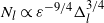 $N_l\propto \varepsilon^{-9/4}\Delta_l^{3/4}$
, which together result in an improved computational complexity of
 $\mathcal{O}(\varepsilon^{-5/2})$
.
4. Numerical results
4.1. Models
4.1.1. Kuramoto model.
We consider the Kuramoto model
 $\{X_t\}_{t\geq0}$
defined by the McKean–Vlasov SDE
 \begin{equation*} {\mathrm{d}} X_t = \bigg(\theta + \int_{\mathbb{R}}\sin(X_t - y)\,{\mathrm{d}}\mu_t(y)\bigg)\,{\mathrm{d}} t + \sigma\,{\mathrm{d}} W_t, \quad X_0 = x_0\in\mathbb{R},\ t\in[0,T],\end{equation*}
where
 $\mu_t$
is the law of
 $X_t$
,
 $\theta$
is a random variable,
 $\sigma>0$
, and
 $T\in\mathbb{N}$
. The Kuramoto model is a well-known mean field game model frequently used for numerical demonstrations. Note that we expect that we can obtain the improved cost of
 $\mathcal{O}(\varepsilon^{-4})$
in this case, since the diffusion coefficient is constant.
4.1.2. Modified Kuramoto model.
In this demonstration consider the process
 $\{X_t\}_{t\geq0}$
satisfying the McKean–Vlasov SDE
 \begin{equation*} {\mathrm{d}} X_t = \bigg(\theta + \int_{\mathbb{R}}\sin(X_t - y)\,{\mathrm{d}}\mu_t(y)\bigg)\,{\mathrm{d}} t + \bigg(\frac{\sigma}{1+X_t^2}\bigg)\,{\mathrm{d}} W_t, \quad X_0 = x_0\in\mathbb{R},\ t\in[0,T],\end{equation*}
where
 $\mu_t$
is the law of
 $X_t$
,
 $\theta$
is a random variable,
 $\sigma>0$
, and
 $T\in\mathbb{N}$
. We call this the modified Kuramoto model. We consider this case since we expect that the non-constant diffusion coefficient should demonstrate our theoretical results in the previous section, in that the computational cost should be
 $\mathcal{O}(\varepsilon^{-4}|\log(\varepsilon)|^2)$
.
4.2. Simulation results
For both models we impose observations
 $\{Y_k\}_{t=1}^T$
at unit times that follow
 $Y_k\mid X_k=x_k \sim \mathcal{N}(x_k, \tau^2)$
for
 $k\in\{1,\dots,T\}$
, and set
 $x_0=1$
,
 $\theta=0$
,
 $\sigma=0.2$
,
 $\tau=1$
, and
 $T=50$
. We simulated a path from each model using Algorithm 1 with level 9 and 5000 particles. We computed the estimator
 $\pi^{L,N,M}_T(\varphi)$
and
 $\widehat{\pi^L_T(\varphi)}$
for the function
 $\varphi(x)=x$
, where M,N were chosen as discussed in Subsection 3.3. In order to calculate the MSEs of the two estimators we considered a proxy ground truth for the filter, obtained by computing
 $\pi^{L,N,M}_T(\varphi)$
at level 7. The MSEs in our simulation were calculated using 128 independent replications.
Figure 1 shows log-log plots for the mean square errors against the theoretical costs for the two filter estimators applied to filtering the Kuramoto model and the modified Kuramoto. In both cases we expect the multilevel methods to have rates of about
 $-2$
(Kuramoto) and
 $-2.2$
, reflecting costs of
 $\mathcal{O}(\varepsilon^{-4})$
and
 $\mathcal{O}(\varepsilon^{-4}|\log(\varepsilon)|^2)$
, and this is exactly what we observe. For the case of the PF (single level), the rate should be about
 $-2.5$
, which gives a cost of
 $\mathcal{O}(\varepsilon^{-5})$
. The plots show the expected improvements of the multilevel method.
Left: Kuramoto model – single-level (SL) for
 $2\leq L\leq 6$
, multi-level (ML) for
 $3\leq L\leq 6$
. Right: Modified Kuramoto model – single-level for
 $2\leq L\leq 6$
, multi-level for
 $3\leq L\leq 6$
.

Appendix A. Proofs
A.1. Structure
This appendix contains several technical results that are used to prove Theorems 1 and 2. We begin with a short section on the additional notation and auxiliary processes that are used. Subsection A.3 is devoted to studying the auxiliary processes
 $\{Z^{l,M,i}\}_{i=1}^M$
, which are defined below. Subsections A.3 and A.4 provide technical results leading to the proof of Lemma 9. Subsection A.5 introduces several further technical results and employs Lemma 9 to ultimately prove Theorem 1. Subection A.6 presents a technical discussion and uses the previously proven results to present a proof for Theorem 2. To understand the appendix, it should be read in the order presented.
A.2. Notation
Let
 $(\Omega,\mathcal{F},\mathbb{P})$
be a measure space,
 $W_t$
a Brownian motion on
 $\Omega$
, and
 $X_t$
the solution of the MVSDE (1). For random variables
 $A_1,\dots,A_n$
and
 $\sigma$
-subalgebras
 $\mathcal{F}_1,\dots\mathcal{F}_n$
we define
 $\sigma(A_1,\dots,A_n,\mathcal{F}_1,\dots,\mathcal{F}_n)$
to be the smallest
 $\sigma$
-subalgebra
 $\mathcal{G}$
of
 $\mathcal{F}$
that contains the set
 $\bigcup_{i=1}^n\mathcal{F}_i$
and that satisfies that the random variables
 $A_1,\dots,A_n$
are measurable with respect to
 $\mathcal{G}$
. We consider step (ii) of Algorithm 5: This step calls Algorithm 3, and step (ii) of Algorithm 5 is called T times. For
 $(l,N,M)\in\mathbb{N}^3$
given, we then use the following associated notation:
-
•
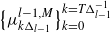
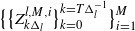
$\big\{\mu_{k\Delta_l}^{l,M}\big\}_{k=0}^{k=T\Delta_l^{-1}}$
and
$\big\{\mu_{k\Delta_{l-1}}^{l-1,M}\big\}_{k=0}^{k=T\Delta_{l-1}^{-1}}$
are the output measures of all the iterations of step (ii) in Algorithm 5. -
•
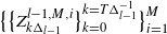
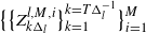
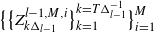
$\big\{\big\{Z_{k\Delta_l}^{l,M,i}\big\}_{k=0}^{k=T\Delta_l^{-1}}\big\}_{i=1}^M$
and
$\big\{\big\{Z_{k\Delta_{l-1}}^{l-1,M,i}\big\}_{k=0}^{k=T\Delta_{l-1}^{-1}}\big\}_{i=1}^M$
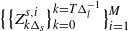
are the particles that generated the outputs of all the iterations of step (ii) in Algorithm 5. Let
$\mathcal{F}^{l,M}_{k\Delta_l} = \sigma\big(\big\{\big\{Z_{j\Delta_l}^{l,M,i}\big\}_{j=0}^{j=k}\big\}_{i=1}^M\big)$
and
$\mathcal{F}^{l-1,M}_{k\Delta_{l-1}}=\sigma\big(\big\{\big\{Z_{j\Delta_{l-1}}^{l-1,M,i}\big\}_{j=0}^{j=k}\big\}_{i=1}^M\big)$
be the respective natural filtrations of these particles. -
•
$\{B^i_t\}_{i=1}^M$
are the Brownian motions generated in all the iterations of step (ii) of Algorithm 5 in order to generate the particles
$\big\{\big\{Z_{k\Delta_l}^{l,M,i}\big\}_{k=1}^{k=T\Delta_l^{-1}}\big\}_{i=1}^M$
and
$\big\{\big\{Z_{k\Delta_{l-1}}^{l-1,M,i}\big\}_{k=1}^{k=T\Delta_{l-1}^{-1}}\big\}_{i=1}^M$
. Write
$\Delta B^{s,i}_t = B^{i}_t - B^{i}_{t-\Delta_s}$
for
$t\in[\Delta_l,T]$
,
$s\in\{l,l-1\}$
, and
$i\in\{1,\dots,M\}$
. Similarly, write
$\Delta W^s_t = W_t - W_{t-\Delta_s}$
for
$t\in[\Delta_l,T]$
and
$s\in\{l,l-1\}$
. -
• For
$s\in\{l-1,l\}$
, define the discrete process
$\big\{\big\{Z_{k\Delta_s}^{s,i}\big\}_{k=0}^{k=T\Delta_l^{-1}}\big\}_{i=1}^M$
as the solution of the equations (4)with
\begin{align} Z_{(k+1)\Delta_s}^{s,i} & = Z_{k\Delta_s}^{s,i} \nonumber \\ & \quad + a\big(Z_{k\Delta_s}^{s,i},\overline{\xi}_1\big(Z_{k\Delta_s}^{s,i},\mu_{k\Delta_s}^{s}\big)\big)\Delta_s + b\big(Z_{k\Delta_s}^{s,i}, \overline{\xi}_2\big(Z_{k\Delta_s}^{s,i},\mu_{k\Delta_s}^{s}\big)\big)\Delta B^{s,i}_{(k+1)\Delta_s}, \end{align}
$\mu^s_{k\Delta_s}$
being the law of
$Z^{s,1}_{k\Delta_s}$
and with the initial condition
$Z^{s,i}_0=x_0$
for every
$(k,i)\in\{0,\dots,T\Delta_s^{-1}-1\}\times\{1,\dots,M\}$
.
-
• For
$s\in\{l-1,l\}$
, define the processes
$\tilde{Z}^{s,M}_t$
and
$\tilde{Z}^{s}_t$
as the solutions of
\begin{align*} \tilde{Z}_{(k+1)\Delta_s}^s & = \tilde{Z}_{k\Delta_s}^s \\ & \quad + a\big(\tilde{Z}_{k\Delta_s}^s,\overline{\xi}_1\big(\tilde{Z}_{k\Delta_s}^s,\mu_{k\Delta_s}^s\big)\big)\Delta_s + b\big(\tilde{Z}_{k\Delta_s}^s, \overline{\xi}_2\big(\tilde{Z}_{k\Delta_s}^s,\mu_{k\Delta_s}^s\big)\big)\Delta W^{s}_{(k+1)\Delta_s}, \\ \end{align*}
with
\begin{align*} \tilde{Z}_{(k+1)\Delta_s}^{s,M} & = \tilde{Z}_{k\Delta_s}^{s,M} \\ & \quad + a\big(\tilde{Z}_{k\Delta_s}^{s,M}, \overline{\xi}_1\big(\tilde{Z}_{k\Delta_s}^{s,M},\mu_{k\Delta_s}^{s,M}\big)\big)\Delta_s + b\big(\tilde{Z}_{k\Delta_s}^{s,M}, \overline{\xi}_2\big(\tilde{Z}_{k\Delta_s}^{s,M},\mu_{k\Delta_s}^{s,M}\big)\big)\Delta W^{s}_{(k+1)\Delta_s}, \end{align*}
$\mu_{k\Delta_s}^s$
being the law of
$Z_{k\Delta_s}^{s,1}$
,
$\mu_{k\Delta_s}^{s,M} = ({1}/{M})\sum_{i=1}^M\delta_{Z_{k\Delta_s}^{s,M,i}}$
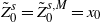
, and with the initial condition
$\tilde{Z}^{s}_0=\tilde{Z}^{s,M}_0=x_0$
for every
$k\in\{0,\dots,T\Delta_{s}^{-1}-1\}$
. Conditioning on the
$\sigma$
-algebra
$\mathcal{F}^{s,M}_t$
, denote by
$P_{\mu_{t-1}^{s,M},t}^{s,M}$
the transition kernel of the process
$\{\tilde{Z}^{s,M}_t\}_{t\in\{0,1,\dots,T\}}$
.
-
• For
$\varphi\in\mathcal{B}(\mathbb{R}^d)$
, define and for
\begin{align*} \gamma_t(\varphi) & \,:\!=\, \int_{\mathbb{R}^{dt}}\varphi(x_t)\Bigg\{\prod_{p=1}^tG(x_p,y_p)\Bigg\} \prod_{p=1}^tP_{\mu_{p-1},p}(x_{p-1},{\mathrm{d}} x_p), \\ \gamma_t^l(\varphi) & \,:\!=\, \int_{\mathbb{R}^{dt}}\varphi(x_t)\Bigg\{\prod_{p=1}^tG(x_p,y_p)\Bigg\} \prod_{p=1}^tP_{\mu_{p-1}^l,p}^l(x_{p-1},{\mathrm{d}} x_p), \end{align*}
$s\in\{l-1,l\}$
define
\begin{align*} \gamma_t^{l,M}(\varphi) \,:\!=\, \int_{\mathbb{R}^{dt}}\varphi(x_t)\Bigg\{\prod_{p=1}^tG(x_p,y_p)\Bigg\} \prod_{p=1}^tP_{\mu_{p-1}^{l,M},p}^{l,M}(x_{p-1},{\mathrm{d}} x_p). \end{align*}
-
• Define
$\pi^{l,M}_t(\varphi) = \gamma^{l,M}_t(\varphi)/\gamma^{l,M}_t(1)$
.























The Brownian motions
 $\{B_t^i\}_{i=1}^M$
and
 $W_t$
are independent. Notice that
 $\gamma_t^{l,M}(\varphi)$
and
 $\gamma_t^{l-1,M}(\varphi)$
are random variables measurable with respect to
 $\sigma(\mathcal{F}^{l-1,M}_t,\mathcal{F}^{l,M}_t)$
. The process
 $\tilde{Z}_t^s$
is the Euler–Maruyama discretization for the process
 $X_t$
. We introduce the process
 $\tilde{Z}_t^{s,M}$
to approximate
 $\tilde{Z}_t^s$
. The process
 $\tilde{Z}_t^{s,M}$
utilizes the particles
 $\{Z_t^{s,M,i}\}_{i=1}^M$
to create an empirical measure that approximates the measure
 $\mu^s_t$
independently of
 $W_t$
. Our main objective is to study the increments
 $\pi_t^{l,N,M}(\varphi)-\pi_t^{l-1,N,M}(\varphi)$
. To achieve this, we investigate the increments
 $Z_t^{l,M,i}-Z_t^{l-1,M,i}$
and
 $\tilde{Z}_t^{l,M}-\tilde{Z}_t^{l-1,M}$
. Finally, we leverage the results obtained and the theory of multi-level particle filters to bound the
 $\mathbb{L}_2$
error of the estimator
 $\widehat{\pi_t^L(\varphi)}$
.
Throughout the following proofs we denote constants by C. For concise notation C may change value from one step to another. Unless explicitly stated, C is independent of l, M, N, and i.
A.3. Bounds on
$\boldsymbol{Z}^{\boldsymbol{l,M,i}}_{\boldsymbol{t}}$
increments

We start by stating two technical lemmata. Lemma 1 is a discrete Grönwall-type inequality, while Lemma 2 is a simple upper bound for the multinomial expansion of the expression
 $\|A+B\|^{2k} = (\|A\|^2 + 2A^{\top}B + \|B\|^2)^k$
. We will refer to Lemma 2 as the
 $C^k$
bound to distinguish it from the popular
 $C^p$
inequality.
Lemma 1. Let
 $\Delta>0$
and let
 $\{u_{k\Delta}\}$
be a sequence of non-negative real numbers indexed by the set
 $\Delta\mathbb{N}_0=\{k\Delta\colon k\in\mathbb{N}_0\}$
. Suppose there exist constants
 $C_1,C_2>0$
for which the following inequality holds for every
 $k\in\mathbb{N}$
:
 $u_{k\Delta} \leq (1+C_1\Delta)u_{(k-1)\Delta} + C_2\Delta$
. Then the following inequality holds for every
 $k\in\mathbb{N}_0$
:
 $u_{k\Delta} \leq e^{k\Delta C_1}(u_0 + k\Delta C_2)$
.
Lemma 2. Let
 $k\in\mathbb{N}$
. There exists
 $C>0$
such that, for all
 $(A,B)\in(\mathbb{R}^d)^2$
the following inequality holds:
 $\|A+B\|^{2k} \leq \|A\|^{2k} + 2k\|A\|^{2k-2}A^{\top}B + C\|B\|^2(\|A\|^{2k-2}+\|B\|^{2k-2})$
.
Lemma 3. Assume Assumption 1 and let
 $k\in\mathbb{N}$
. There exists a constant
 $C<+\infty$
such that, for every
 $(l,M)\in\mathbb{N}_0\times\mathbb{N}$
,
 $t\in\{0,\Delta_l,\dots,T\}$
, and
 $i\in\{1,\dots,M\}$
,
 \begin{equation*} \max\{\mathbb{E}[\|Z^{l,M,i}_t\|^k], \mathbb{E}[\|Z^{l,i}_t\|^k]\}\leq C. \end{equation*}
Proof. It is enough to prove the inequality for even positive integers k, the general case following from the inequality
 $\mathbb{E}[\|A\|^{k}] \leq \mathbb{E}[\|A\|^{2k}]^{1/2}$
for any
 $\mathbb{R}^d$
-valued random variable A. Using the definition (4) of
 $Z^{l,i}_t$
, applying the
 $C^k$
bound (Lemma 2) twice, using Assumption 1 that the functions a,b are bounded,
 $\Delta_l\leq 1$
,
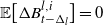 $\mathbb{E}\big[\Delta B^{l,i}_{t-\Delta_l}\big]=0$
, and
 $\mathbb{E}\big[\big\|B^{l,i}_{t-\Delta_l}\big\|^k\big]\leq C\Delta_l^{k/2}$
, we have
 \begin{align*} \mathbb{E}[\|Z^{l,i}_{t}\|^k] & = \mathbb{E}\big[\big\|Z^{l,i}_{t-\Delta_l} + a\big(Z^{l,i}_{t-\Delta_l},\bar{\xi}_2\big(Z^{l,i}_{t-\Delta_l},\mu^{l}_{t-\Delta_l}\big)\big)\Delta_l \\[3pt] & \quad + b\big(Z^{l,i}_{t-\Delta_l},\bar{\xi}_2\big(Z^{l,i}_{t-\Delta_l},\mu^{l}_{t-\Delta_l}\big)\big) \Delta B^{l,i}_{t-\Delta_l}\big\|^k\big] \\[3pt] & \leq \mathbb{E}\big[\big\|Z^{l,i}_{t-\Delta_l}\big\|^k\big] + C\Delta_l\max_{r\in\{1,2,3,4\}}\mathbb{E}\big[\big\|Z^{l,i}_{t-\Delta_l}\big\|^{k-r}\big] + C\Delta_l^{k/2} \\[3pt] & \leq (1+C\Delta_l)\mathbb{E}\big[\big\|Z^{l,i}_{t-\Delta_l}\big\|^{k}\big] + C\Delta_l. \end{align*}
The last line follows from the inequality
 $x^s\leq 1+x^k$
for
 $0\leq s\leq k$
and
 $x\geq0$
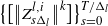
. Applying Grönwall’s inequality (Lemma 1) to the sequence
 $\big\{\big[\big\|Z^{l,i}_{s\Delta_l}\big\|^{k}\big]\big\}_{s=0}^{T/\Delta_l}$
yields the inequality
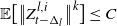 $\mathbb{E}\big[\big\|Z^{l,i}_{t-\Delta_l}\big\|^{k}\big] \leq C$
; clearly, following similar steps yields
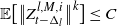 $\mathbb{E}\big[\big\|Z^{l,M,i}_{t-\Delta_l}\big\|^{k}\big] \leq C$
.
Lemma 4. Assume Assumption 1 and let
 $k\in\mathbb{N}$
. There exists a constant
 $C<+\infty$
such that, for every
 $(l,M)\in\mathbb{N}_0\times\mathbb{N}$
,
 $t\in\{0,\Delta_l,\dots,T\}$
, and
 $i\in\{1,\dots,M\}$
,
 \begin{align*} \mathbb{E}\big[\big\|Z^{l,M,i}_t-Z^{l,i}_t\big\|^k\big] & \leq C\frac{1}{M^{k/2}}, \\ \mathbb{E}\big[\big\|Z^{l,M,i}_t-Z^{l-1,M,i}_t\big\|^k\big] & \leq C\Delta_l^{k/2}, \end{align*}
where the convention
 $Z^{-1,M,i} = 0$
is used.
Proof. Let
 $t\in \{\Delta_l,2\Delta_l,\dots,T\}$
. Then
 \begin{align} Z^{l,M,i}_t - Z^{l,i}_t & = Z^{l,M,i}_{t-\Delta_l} - Z^{l,i}_{t-\Delta_l} \nonumber \\ & \quad + \big[a\big(Z^{l,M,i}_{t-\Delta_l},\bar{\xi}_1\big(Z^{l,M,i}_{t-\Delta_l},\mu^{l,M}_{t-\Delta_l}\big)\big) - a\big(Z^{l,i}_{t-\Delta_l},\bar{\xi}_1\big(Z^{l,i}_{t-\Delta_l},\mu^{l}_{t-\Delta_l}\big)\big)\big]\Delta_l \nonumber \\ & \quad + [b\big(Z^{l,M,i}_{t-\Delta_l},\bar{\xi}_2\big(Z^{l,M,i}_{t-\Delta_l},\mu^{l,M}_{t-\Delta_l}\big)\big) - b\big(Z^{l,i}_{t-\Delta_l},\bar{\xi}_2\big(Z^{l,i}_{t-\Delta_l},\mu^{l}_{t-\Delta_l}\big)\big)]\Delta B^{l,i}_t. \end{align}
Using the
 $C^p$
inequality and that the functions a and
 $\xi_1$
are bounded and Lipschitz (Assumption 1), there exists a constant
 $C>0$
that satisfies
 \begin{align} & \mathbb{E}\big[\big\|a\big(Z^{l,M,i}_{t-\Delta_l}, \bar{\xi}_1\big(Z^{l,M,i}_{t-\Delta_l},\mu^{l,M,i}_{t-\Delta_l}\big)\big) - a\big(Z^{l,i}_{t-\Delta_l}, \bar{\xi}_1\big(Z^{l,i}_{t-\Delta_l},\mu^{l,i}_{t-\Delta_l}\big)\big)\big\|^k\big] \nonumber \\ & \leq C\Bigg(\mathbb{E}\big[\big\|Z^{l,M,i}_{t-\Delta_l} - Z^{l,i}_{t-\Delta_l}\big\|^k\big] + \mathbb{E}\Bigg[\Bigg|\frac{1}{M}\sum_{j=1}^M\xi_1\big(Z^{l,M,i}_{t-\Delta_l}Z^{l,M,j}_{t-\Delta_l}\big) - \frac{1}{M}\sum_{j=1}^M\xi_1\big(Z^{l,i}_{t-\Delta_l},Z^{l,j}_{t-\Delta_l}\big)\Bigg|^k\Bigg] \nonumber \\ & \quad + \frac{1}{M^k}\mathbb{E}\Bigg[\Bigg|\sum_{j=1,\,j\not=i}^M\bigg(\xi_1(Z^{l,i}_{t-\Delta_l},Z^{l,j}_{t-\Delta_l}) - \int\xi_1\big(Z^{l,i}_{t-\Delta_l},y\big)\,{\mathrm{d}}\mu^l_{t-\Delta_l}(y)\bigg)\Bigg|^k\Bigg]\Bigg) + C\frac{1}{M^k}. \end{align}
By the
 $C^p$
inequality, the second term after the inequality is bounded by
 \begin{align*} \frac{1}{M}\sum_{j=1}^M\mathbb{E}\big[\big|\xi_1\big(Z^{l,M,i}_{t-\Delta_l}Z^{l,M,j}_{t-\Delta_l}\big) - \xi_1(Z^{l,i}_{t-\Delta_l},Z^{l,j}_{t-\Delta_l})\big|^k\big] \leq C\sup\nolimits_q\mathbb{E}\big[\big\|Z^{l,M,q}_{t-\Delta_l} - Z^{l,q}_{t-\Delta_l}\big\|^k\big]. \end{align*}
For the third term we use the independence of
 $Z_t^{l,i}$
and
 $Z_t^{l,j}$
for
 $i\not=j$
, Fubini’s Theorem, and the Marcinkiewicz–Zygmund inequality. Let
 $p\in[1,\infty)$
and
 $X_1,\dots,X_n$
be zero-mean,
 $L^p$
, and independent random variables. Then there exists a constant
 $C(p)>0$
that satisfies
 $\mathbb{E}\big[\big|\sum_{i=1}^nX_i\big|^p\big] \leq C(p)\mathbb{E}\big[\big(\sum_{i=1}^n|X_i|^2\big)^{p/2}\big]$
, and
 \begin{align} & \mathbb{E}\Bigg[\Bigg|\sum_{j=1,\,j\not=i}^M\bigg(\xi_1\big(Z^{l,i}_{t-\Delta_l},Z^{l,j}_{t-\Delta_l}\big) - \int\xi_1\big(Z^{l,i}_{t-\Delta_l},y\big)\,{\mathrm{d}}\mu^l_{t-\Delta_l}(y)\bigg)\Bigg|^k\Bigg] \nonumber \\ & \qquad = \int\mathbb{E}\Bigg[\Bigg|\sum_{j=1,\,j\not=i}^M\bigg(\xi_1\big(z,Z^{l,j}_{t-\Delta_l}\big) - \int\xi_1(z,y)\,{\mathrm{d}}\mu^l_{t-\Delta_l}(y)\bigg)\Bigg|^k\Bigg]\,{\mathrm{d}}\mu^l_{t-\Delta_l}(z) \nonumber \\ & \qquad \leq C\int\mathbb{E}\Bigg[\Bigg(\sum_{j=1.\,j\not=i}^M\bigg(\xi_1\big(z,Z^{l,j}_{t-\Delta_l}\big) - \int\xi_1(z,y)\,{\mathrm{d}}\mu^l_{t-\Delta_l}(y)\bigg)^2\Bigg)^{k/2}\Bigg]\,{\mathrm{d}}\mu^l_{t-\Delta_l}(z) \nonumber \\ & \qquad \leq CM^{k/2}, \end{align}
where the last line follows from the boundedness of
 $\xi_1$
. Thus, we have shown that
 \begin{eqnarray} \mathbb{E}\big[\big\|a\big(Z^{l,M,i}_{t-\Delta_l}, \bar{\xi}_1\big(Z^{l,M,i}_{t-\Delta_l},\mu^{l,M,i}_{t-\Delta_l}\big)\big)& -& a\big(Z^{l,i}_{t-\Delta_l},\bar{\xi}_1\big(Z^{l,i}_{t-\Delta_l},\mu^{l,i}_{t-\Delta_l}\big)\big)\|^k\big] \nonumber\\&\leq & C\sup\nolimits_q\mathbb{E}\big[\big\|Z^{l,M,q}_{t-\Delta_l} - Z^{l,q}_{t-\Delta_l}\big\|^k\big] + C\frac{1}{M^{k/2}}. \end{eqnarray}
A similar bound holds for the function b. Analogously to the proof of Lemma 3, we apply the
 $C^k$
bound (Lemma 2) twice on
 $\big\|Z^{l,M,i}_{t}-Z^{l,i}_{t}\big\|$
following (5), and using the bound (8) (for both a and b) yields
 \begin{equation*} \sup\nolimits_q\mathbb{E}[\|Z^{l,M,q}_{t} - Z^{l,q}_{t}\|^k] \leq (1+C\Delta_l)\sup\nolimits_q\mathbb{E}\big[\big\|Z^{l,M,q}_{t-\Delta_l} - Z^{l,q}_{t-\Delta_l}\big\|^k\big] + C\Delta_l\frac{1}{M^{k/2}}. \end{equation*}
Applying Grönwall’s inequality (Lemma 1) to the sequence
 $\big\{\sup\nolimits_q\mathbb{E}\big[\big\|Z^{l,M,q}_{s\Delta_l}-Z^{l,q}_{s\Delta_l}\big\|^k\big]\big\}_{s=0}^{T/\Delta_l}$
and using
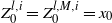 $Z^{l,i}_0=Z^{l,M,i}_0=x_0$
proves the first inequality. For the second inequality in the lemma statement, we write
 \begin{align} & Z^{l,M,i}_{t} - Z^{l-1,M,i}_{t} \nonumber \\[3pt] & \quad = Z^{l,M,i}_{t-\Delta_{l-1}} - Z^{l-1,M,i}_{t-\Delta_{l-1}} \nonumber \\[4pt] & \qquad + \big(a\big(Z^{l,M,i}_{t-\Delta_{l-1}}, \bar{\xi}_{1}\big(Z^{l,M,i}_{t-\Delta_{l-1}}, \mu^{l,M}_{t-\Delta_{l-1}}\big)\big) - a\big(Z^{l-1,M,i}_{t-\Delta_{l-1}}, \bar{\xi}_{1}\big(Z^{l-1,M,i}_{t-\Delta_{l-1}}, \mu^{l-1,M}_{t-\Delta_{l-1}}\big)\big)\big)\Delta_{l-1} \nonumber \\[4pt] & \qquad + \big(b\big(Z^{l,M,i}_{t-\Delta_{l-1}}, \bar{\xi}_{2}\big(Z^{l,M,i}_{t-\Delta_{l-1}}, \mu^{l,M}_{t-\Delta_{l-1}}\big)\big) - b\big(Z^{l-1,M,i}_{t-\Delta_{l-1}}, \bar{\xi}_{2}\big(Z^{l-1,M,i}_{t-\Delta_{l-1}},\mu^{l-1,M}_{t-\Delta_{l-1}}\big)\big)\big)\Delta B^{l-1,i}_{t} \nonumber \\[4pt] & \qquad + \big(a\big(Z^{l,M,i}_{t-\Delta_{l}}, \bar{\xi}_{1}\big(Z^{l,M,i}_{t-\Delta_{l}}, \mu^{l,M}_{t-\Delta_{l}}\big)\big) - a\big(Z^{l,M,i}_{t-\Delta_{l-1}}, \bar{\xi}_{1}\big(Z^{l,M,i}_{t-\Delta_{l-1}}, \mu^{l,M}_{t-\Delta_{l-1}}\big)\big)\big)\Delta_{l} \nonumber \\[4pt] & \qquad + \big(b\big(Z^{l,M,i}_{t-\Delta_{l}}, \bar{\xi}_{2}\big(Z^{l,M,i}_{t-\Delta_{l}}, \mu^{l,M}_{t-\Delta_{l}}\big)\big) - b\big(Z^{l,M,i}_{t-\Delta_{l-1}}, \bar{\xi}_{2}\big(Z^{l,M,i}_{t-\Delta_{l-1}}, \mu^{l,M}_{t-\Delta_{l-1}}\big)\big)\big)\Delta B^{l,i}_{t}. \end{align}
Bounding each term following the same technique used to prove the first inequality in the lemma statement, we can show the following inequality:
 \begin{align*} & \sup\nolimits_i\mathbb{E}[\|Z^{l,M,i}_{t} - Z^{l-1,M,i}_{t}\|^k] \\ & \leq (1+C\Delta_l)\sup\nolimits_i\mathbb{E}\big[\big\|Z^{l,M,i}_{t-\Delta_{l-1}} - Z^{l-1,M,i}_{t-\Delta_{l-1}}\big\|^k\big] + C\Delta_{l-1}\big(\sup\nolimits_i\mathbb{E}\big[\big\|Z^{l,M,i}_{t-\Delta_{l}} - Z^{l,M,i}_{t-\Delta_{l-1}}\big\|^k\big] + \Delta_{l-1}^{k/2}\big). \end{align*}
From the definition of
 $Z^{l,M,i}_t$
and the boundedness of a and b, we have
 $\sup\nolimits_i\mathbb{E}\big[\big\|Z^{l,M,i}_{t-\Delta_{l}}-Z^{l,M,i}_{t-\Delta_{l-1}}\big\|^k\big] \leq C\Delta_l^{k/2}$
. The proof then follows similarly to the proof of the first inequality in the lemma statement by applying Grönwall’s inequality (Lemma 1) to the sequence
 $\big\{\sup\nolimits_i\mathbb{E}\big[\big\|Z^{l,M,i}_{s\Delta_{l-1}} - Z^{l-1,M,i}_{s\Delta_{l-1}}\big\|^k\big]\big\}_{s=0}^{T/\Delta_{l-1}}$
.
Lemma 5. Let
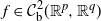 $f\in\mathcal{C}_\mathrm{b}^2(\mathbb{R}^p,\mathbb{R}^q)$
. There exists a constant
 $C<+\infty$
such that the following inequality holds for every
 $(x,y,z,w)\in(\mathbb{R}^p)^4$
:
 \begin{equation*} \|f(x)-f(y)-f(z)+f(w)\|\leq C\|x-y-z+w\| + C\|z-w\|(\|z-x\|+\|w-y\|). \end{equation*}
Proof. We use the formula
 \begin{align*} f(x)-f(y)-f(z)+f(w) & = (x-y-z+w)^{\top}\int_0^1\nabla f(tx+(1-t)y)\,{\mathrm{d}} t \\ & \quad + (z-w)^{\top}\int_0^1(\nabla f(tx+(1-t)y)-\nabla f(tz+(1-t)w))\,{\mathrm{d}} t. \end{align*}
The bound follows by employing the boundedness of the first two derivatives of f, the Cauchy–Schwarz inequality, and the inequality
 $\|t(x-z) + (1-t)(y-w)\|\leq \|z-x\| + \|w-y\|$
.
Lemma 6. Assume Assumption 1, and let
 $k\in\mathbb{N}$
. There exists a constant
 $C<+\infty$
such that, for every
 $(l,M)\in\mathbb{N}\times\mathbb{N}$
,
 $t\in\{0,\Delta_l,\dots,T\}$
, and
 $i\in\{1,\dots,M\}$
,
 \begin{equation*} \mathbb{E}\big[\big\|Z^{l,M,i}_t - Z^{l-1,M,i}_t - Z^{l,i}_t + Z^{l-1,i}_t\big\|^k\big] \leq C\Delta_l^{k/2}/M^{k/2}. \end{equation*}
Proof. Assume k is even. The inequality is proven following the same strategy as the proof of Lemma 4, so we write, following (5) and (9),
 \begin{align} & Z^{l,M,i}_{t} - Z^{l-1,M,i}_{t} - Z^{l,i}_{t} + Z^{l-1,i}_{t} \nonumber \\[3pt]& = Z^{l,M,i}_{t-\Delta_{l-1}} - Z^{l-1,M,i}_{t-\Delta_{l-1}} - Z^{l,i}_{t-\Delta_{l-1}} + Z^{l-1,i}_{t-\Delta_{l-1}} \nonumber \\[3pt]& \quad + \big[a\big(Z^{l,M,i}_{t-\Delta_{l-1}}, \bar{\xi}_{1}\big(Z^{l,M,i}_{t-\Delta_{l-1}}, \mu^{l,M}_{t-\Delta_{l-1}}\big)\big) - a\big(Z^{l-1,M,i}_{t-\Delta_{l-1}}, \bar{\xi}_{1}\big(Z^{l-1,M,i}_{t-\Delta_{l-1}}, \mu^{l-1,M}_{t-\Delta_{l-1}}\big)\big) \nonumber \\[3pt] & \quad - a\big(Z^{l,i}_{t-\Delta_{l-1}}, \bar{\xi}_{1}\big(Z^{l,i}_{t-\Delta_{l-1}}, \mu^{l}_{t-\Delta_{l-1}}\big)\big) + a\big(Z^{l-1,i}_{t-\Delta_{l-1}}, \bar{\xi}_{1}\big(Z^{l-1,i}_{t-\Delta_{l-1}}, \mu^{l-1}_{t-\Delta_{l-1}}\big)\big)\big]\Delta_{l-1} \nonumber \\[3pt] & \quad + \cdots, \end{align}
where
 $\cdots$
indicates that the rest of the terms are similar to the first term in (10) and follow the same general form as (5) and (9). We will show how to bound the first term in (10), since the
 $\cdots$
terms are treated similarly. Define the vector
 $R^{l,M} = \big(Z^{l,M,i}_{t-\Delta_{l-1}},\bar{\xi}_{1}\big(Z^{l,M,i}_{t-\Delta_{l-1}},\mu^{l,M}_{t-\Delta_{l-1}}\big)\big)$
and write
 $a(R^{l,M})$
for
 $a\big(Z^{l,M,i}_{t-\Delta_{l-1}},\bar{\xi}_{1}\big(Z^{l,M,i}_{t-\Delta_{l-1}},\mu^{l,M}_{t-\Delta_{l-1}}\big)\big)$
; similarly define
 $R^{l-1,M}$
,
 $R^{l}$
, and
 $R^{l-1}$
. Applying Lemma 5 to the function a, we have
 \begin{align} & \|a(R^{l,M}) - a(R^{l-1,M}) - a(R^{l}) + a(R^{l-1})\| \nonumber \\[5pt] & \leq C\|R^{l,M} - R^{l-1,M}\|(\|R^{l,M} - R^{l}\|+\|R^{l-1,M} - R^{l-1}\|) + C\|R^{l,M} - R^{l-1,M} - R^{l} + R^{l-1}\|. \end{align}
Using the assumption that
 $\xi_1$
is Lipschitz, Lemma 4, and Marcinkiewicz–Zygmund in a manner similar to (7), we have
 $\mathbb{E}[\|R^{l,M}-R^{l-1,M}\|^{2k}] \leq C\Delta_l^{k}$
and
 $\mathbb{E}[\|R^{l,M}-R^{l}\|^{2k}] \leq C/{M^{k}}$
. Thus, using Cauchy–Schwarz and the
 $C^p$
inequality we have
 \begin{align} & \mathbb{E}[\|R^{l,M} - R^{l-1,M}\|^k(\|R^{l,M} - R^{l}\|+\|R^{l-1,M} - R^{l-1}\|)^k] \nonumber \\[5pt] & \leq C(\mathbb{E}[\|R^{l,M} - R^{l,M}\|^{2k}](\mathbb{E}[\|R^{l,M} - R^{l}\|^{2k}] + \mathbb{E}[\|R^{l-1,M} - R^{l-1}\|^{2k}]))^{1/2} \leq C\Delta_l^{k/2}/M^{k/2}. \end{align}
Similarly to (6), the term
 $\|R^{l,M} - R^{l-1,M} - R^{l} + R^{l-1}\|$
in (11) is bounded by
 \begin{align} & \mathbb{E}[\|R^{l,M} - R^{l-1,M} - R^{l} + R^{l-1}\|^k] \nonumber \\[5pt] & \leq C\mathbb{E}\big[\big\|Z_{t-\Delta_{l-1}}^{l,M,i} - Z_{t-\Delta_{l-1}}^{l-1,M,i} - Z_{t-\Delta_{l-1}}^{l,i} + Z_{t-\Delta_{l-1}}^{l-1,i}\big\|^k\big] \nonumber \\[5pt] & \quad + C\mathbb{E}\Bigg[\Bigg|\frac{1}{M}\sum_{j=1}^M \Big(\xi_{1}\big(Z^{l,M,i}_{t-\Delta_{l-1}}, Z^{l,M,j}_{t-\Delta_{l-1}}\big) - \xi_{1}\big(Z^{l-1,M,i}_{t-\Delta_{l-1}}, Z^{l-1,M,j}_{t-\Delta_{l-1}}\big) - \xi_{1}\big(Z^{l,i}_{t-\Delta_{l-1}}, Z^{l,j}_{t-\Delta_{l-1}}\big) \nonumber \\[5pt] & \kern35pt\quad + \xi_{1}\big(Z^{l,i}_{t-\Delta_{l-1}}, Z^{l,j}_{t-\Delta_{l-1}}\big)\Big)\Bigg|^k\Bigg] \nonumber \\[5pt] & \quad + C\mathbb{E}\Bigg[\Bigg|\frac{1}{M}\sum_{j\not=i} \Big(\xi_{1}\big(Z^{l,i}_{t-\Delta_{l-1}}, Z^{l,j}_{t-\Delta_{l-1}}\big) - \xi_{1}\big(Z^{l-1,i}_{t-\Delta_{l-1}}, Z^{l-1,j}_{t-\Delta_{l-1}}\big) \nonumber \\[5pt] & \kern35pt\quad - \int\xi_{1}\big(Z^{l,i}_{t-\Delta_{l-1}}, y\big)\,{\mathrm{d}}\mu^{l}_{t-\Delta_{l-1}}(y) + \int\xi_{1}\big(Z^{l-1,i}_{t-\Delta_{l-1}}, y\big)\,{\mathrm{d}}\mu^{l-1}_{t-\Delta_{l-1}}(y)\Big)\Bigg|^k\Bigg] \nonumber \\[5pt] & \quad + \frac{C}{M^k}\mathbb{E}\Bigg[\Bigg| \xi_{1}\big(Z^{l,i}_{t-\Delta_{l-1}}, Z^{l,i}_{t-\Delta_{l-1}}\big) - \xi_{1}\big(Z^{l-1,i}_{t-\Delta_{l-1}}, Z^{l-1,i}_{t-\Delta_{l-1}}\big) \nonumber \\[5pt] & \kern43pt\quad - \int\xi_{1}\big(Z^{l,i}_{t-\Delta_{l-1}}, y\big)\,{\mathrm{d}}\mu^{l}_{t-\Delta_{l-1}}(y) + \int\xi_{1}\big(Z^{l-1,i}_{t-\Delta_{l-1}}, y\big)\,{\mathrm{d}}\mu^{l-1}_{t-\Delta_{l-1}}(y)\Bigg|^k\Bigg]. \end{align}
Using Lemmata 5 and 4, and Cauchy–Schwarz similarly to (12), the second expectation after the inequality in (13) can be bounded from above by
 \begin{align*} C\sup\nolimits_q\mathbb{E}\big[\big\|Z_{t-\Delta_{l-1}}^{l,M,q} - Z_{t-\Delta_{l-1}}^{l-1,M,q} - Z_{t-\Delta_{l-1}}^{l,q} + Z_{t-\Delta_{l-1}}^{l-1,q}\big\|^k\big] + C\Delta_l^{k/2}/M^{k/2}. \end{align*}
For the third expectation we use Fubini and the Marcinkiewicz–Zygmund inequality in a manner similar to (7),
 $\xi_1$
being Lipschitz, and Lemma 4:
 \begin{align*} & \mathbb{E}\Bigg[\Bigg|\sum_{j\not=i} \Big(\xi_{1}\big(Z^{l,i}_{t-\Delta_{l-1}}, Z^{l,j}_{t-\Delta_{l-1}}\big) - \xi_{1}\big(Z^{l-1,i}_{t-\Delta_{l-1}}, Z^{l-1,j}_{t-\Delta_{l-1}}\big) \\[5pt] & \kern8pt\quad - \int\xi_{1}\big(Z^{l,i}_{t-\Delta_{l-1}}, y\big)\,{\mathrm{d}}\mu^{l}_{t-\Delta_{l-1}}(y) + \int\xi_{1}\big(Z^{l-1,i}_{t-\Delta_{l-1}}, y\big)\,{\mathrm{d}}\mu^{l-1}_{t-\Delta_{l-1}}(y)\Big)\Bigg|^k\Bigg] \\[5pt] & \leq C\mathbb{E}\Bigg[\Bigg|\sum_{j\not=i} \Big(\xi_{1}\big(Z^{l,i}_{t-\Delta_{l-1}}, Z^{l,j}_{t-\Delta_{l-1}}\big) - \xi_{1}\big(Z^{l-1,i}_{t-\Delta_{l-1}}, Z^{l-1,j}_{t-\Delta_{l-1}}\big) \\[5pt] & \kern25pt\quad - \mathbb{E}\big[\xi_{1}\big(Z^{l,i}_{t-\Delta_{l-1}}, Z^{l,j}_{t-\Delta_{l-1}}\big)\big] + \mathbb{E}\big[\xi_{1}\big(Z^{l-1,i}_{t-\Delta_{l-1}}, Z^{l-1,j}_{t-\Delta_{l-1}}\big)\big]\Big)^2\Bigg|^{k/2}\Bigg] \\[5pt] & \leq CM^{k/2}\sup\nolimits_q\mathbb{E}\big[\big\|Z^{l,q}_{t-\Delta_{l-1}}-Z^{l-1,q}_{t-\Delta_{l-1}}\big\|^k\big] \\[5pt] & \leq CM^{k/2}\Delta_{l}^{k/2}. \end{align*}
Using that
 $\xi_1$
is Lipschitz along with Lemma 4, the last expectation in (13) is bounded by
 $C\Delta_l^{k/2}/M^k$
. Therefore, we have shown that
 \begin{align*} & \mathbb{E}\Big[\Big\|a\big(Z^{l,M,i}_{t-\Delta_{l-1}}, \bar{\xi}_{1}\big(Z^{l,M,i}_{t-\Delta_{l-1}}, \mu^{l,M}_{t-\Delta_{l-1}}\big)\big) - a\big(Z^{l-1,M,i}_{t-\Delta_{l-1}}, \bar{\xi}_{1}\big(Z^{l-1,M,i}_{t-\Delta_{l-1}}, \mu^{l-1,M}_{t-\Delta_{l-1}}\big)\big) \\[5pt] & \quad - a\big(Z^{l,i}_{t-\Delta_{l-1}}, \bar{\xi}_{1}\big(Z^{l,i}_{t-\Delta_{l-1}}, \mu^{l}_{t-\Delta_{l-1}}\big)\big) + a\big(Z^{l-1,i}_{t-\Delta_{l-1}}, \bar{\xi}_{1}\big(Z^{l-1,i}_{t-\Delta_{l-1}}, \mu^{l-1}_{t-\Delta_{l-1}}\big)\big)\Big\|^k\Big] \\[5pt] & \leq C\sup\nolimits_q\mathbb{E}\big[\big\|Z^{l,M,q}_{t-\Delta_{l-1}} - Z^{l-1,M,q}_{t-\Delta_{l-1}} - Z^{l,q}_{t-\Delta_{l-1}} + Z^{l-1,q}_{t-\Delta_{l-1}}\big\|^k\big] + C\frac{\Delta_l^{k/2}}{M^{k/2}}. \end{align*}
A similar bound holds for the rest of terms in (10). Applying the
 $C^k$
bound (Lemma 2) several times, we have
 \begin{multline*} \sup\nolimits_i\mathbb{E}[\|Z^{l,M,i}_{t} - Z^{l-1,M,i}_{t} - Z^{l,i}_{t} + Z^{l-1,i}_{t}\|^k] \\[5pt] \leq (1+C\Delta_{l})\sup\nolimits_i\mathbb{E}\big[\big\|Z^{l,M,i}_{t-\Delta_{l-1}} - Z^{l-1,M,i}_{t-\Delta_{l-1}} - Z^{l,i}_{t-\Delta_{l-1}} + Z^{l-1,i}_{t-\Delta_{l-1}}\big\|^k\big] + C\frac{\Delta_l^{k/2}}{M^{k/2}}. \end{multline*}
Finally, applying Grönwall’s inequality to the sequence
 $\big\{\sup\nolimits_i\mathbb{E}\big[\big\|Z^{l,M,i}_{s\Delta_{l-1}} - Z^{l-1,M,i}_{s\Delta_{l-1}} - Z^{l,i}_{s\Delta_{l-1}} + Z^{l-1,i}_{s\Delta_{l-1}}\big\|^k\big]\big\}_{s=0}^{T\Delta_{l-1}^{-1}}$
finishes the proof.
A.4. Bounds on
$\tilde{\boldsymbol{Z}}^{\boldsymbol{l,M}}_t$
and
$\pi^{\boldsymbol{l,N,M}}_t$
increments


Lemma 7. Assume Assumption 1, and let
 $k\in\mathbb{N}$
. There exists a constant
 $C<+\infty$
such that, for every
 $(l,M)\in\mathbb{N}\times\mathbb{N}$
and
 $t\in\{0,\Delta_l,\dots,T\}$
, the following inequalities hold:
 \begin{align*} \max\big\{\mathbb{E}\big[\big\|\tilde{Z}^{l,M}_t\big\|^k\big], \mathbb{E}[\|\tilde{Z}^{l}_t\|^k]\big\} & \leq C, \\[5pt] \mathbb{E}\big[\big\|\tilde{Z}^{l,M}_t - \tilde{Z}^{l}_t\big\|^k\big] & \leq C\frac{1}{M^{k/2}}, \\[5pt] \mathbb{E}\big[\big\|\tilde{Z}^{l,M}_{t} - \tilde{Z}^{l-1,M}_{t}\big\|^k\big] & \leq C\Delta_l^{k/2} , \\[5pt] \mathbb{E}\big[\big\|\tilde{Z}^{l,M}_{t}-\tilde{Z}^{l-1,M}_{t}-\tilde{Z}^{l}_{t}+\tilde{Z}^{l-1}_{t}\big\|^k\big] & \leq C\frac{\Delta_l^{k/2}}{M^{k/2}}. \end{align*}
Proof. We assume k is even. We will prove the second inequality only, since the same technique we use and the techniques used for proving Lemmata 4 and 6 can be applied directly to prove the other inequalities in this lemma. We write
 \begin{align*} \tilde{Z}^{l,M}_t - \tilde{Z}^{l}_t & = \tilde{Z}^{l,M}_{t-\Delta_l} - \tilde{Z}^{l}_{t-\Delta_l} \\[5pt] & \quad + \big[a\big(\tilde{Z}^{l,M}_{t-\Delta_l}, \bar{\xi}_1\big(\tilde{Z}^{l,M}_{t-\Delta_l},\mu^{l,M}_{t-\Delta_l}\big)\big) - a\big(\tilde{Z}^{l}_{t-\Delta_l}, \bar{\xi}_1\big(\tilde{Z}^{l}_{t-\Delta_l},\mu^{l}_{t-\Delta_l}\big)\big)\big]\Delta_l \\[5pt] & \quad + \big[b\big(\tilde{Z}^{l,M}_{t-\Delta_l}, \bar{\xi}_2\big(\tilde{Z}^{l,M}_{t-\Delta_l},\mu^{l,M}_{t-\Delta_l}\big)\big) - b\big(\tilde{Z}^{l}_{t-\Delta_l}, \bar{\xi}_2\big(\tilde{Z}^{l}_{t-\Delta_l},\mu^{l}_{t-\Delta_l}\big)\big)\big]\Delta W^l_t. \end{align*}
The functions a and
 $\xi_1$
are Lipschitz from Assumption 1. Hence, for a constant C we have
 \begin{align} & \mathbb{E}\big[\big\|a\big(\tilde{Z}^{l,M}_{t-\Delta_l}, \bar{\xi}_1\big(\tilde{Z}^{l,M}_{t-\Delta_l},\mu^{l,M}_{t-\Delta_l}\big)\big) - a\big(\tilde{Z}^{l}_{t-\Delta_l}, \bar{\xi}_1\big(\tilde{Z}^{l}_{t-\Delta_l},\mu^{l}_{t-\Delta_l}\big)\big)\big\|^k\big] \nonumber \\[5pt] & \quad \leq C\Bigg(\mathbb{E}\big[\big\|\tilde{Z}^{l,M}_{t-\Delta_l}-\tilde{Z}^{l}_{t-\Delta_l}\big\|^k\big] + \mathbb{E}\Bigg[\Bigg|\frac{1}{M}\sum_{i=1}^M\xi_1\big(\tilde{Z}^{l,M}_{t-\Delta_l},Z^{l,M,i}_{t-\Delta_l}\big) - \frac{1}{M}\sum_{i=1}^M\xi_1\big(\tilde{Z}^{l}_{t-\Delta_l},Z^{l,i}_{t-\Delta_l}\big)\Bigg|^k\Bigg] \nonumber \\[5pt] & \kern25pt \quad + \mathbb{E}\Bigg[\Bigg|\frac{1}{M}\sum_{i=1}^M \xi_1\big(\tilde{Z}^{l}_{t-\Delta_l},Z^{l,i}_{t-\Delta_l}\big) - \int\xi_1\big(\tilde{Z}^{l}_{t-\Delta_l},y\big)\,{\mathrm{d}}\mu^l_{t-\Delta_l}(y)\Bigg|^k\Bigg]\Bigg). \end{align}
The second expectation after the inequality in (14) is bounded by
 $C\big(\mathbb{E}\big[\big\|\tilde{Z}^{l,M}_{t-\Delta_l}-\tilde{Z}^{l}_{t-\Delta_l}\big\|^k\big] + \sup\nolimits_q\mathbb{E}\big[\big\|Z^{l,M,q}_{t-\Delta_l}-Z^{l,q}_{t-\Delta_l}\big\|^k\big]\big)$
and, from Lemma 4, we have
 $\sup\nolimits_q\mathbb{E}\big[\big\|Z^{l,M,q}_{t-\Delta_l}-Z^{l,q}_{t-\Delta_l}\big\|^k\big] \leq C/M^{k/2}$
. The third expectation after the inequality in (14) is bounded above by
 $C/M^{k/2}$
using Fubini and the Marcinkiewicz–Zygmund inequality in a manner similar to (7). Therefore, we have
 \begin{eqnarray*} \mathbb{E}\Big[\Big\|a\Big(\tilde{Z}^{l,M}_{t-\Delta_l}, \bar{\xi}_1\Big(\tilde{Z}^{l,M}_{t-\Delta_l},\mu^{l,M}_{t-\Delta_l}\Big)\Big) &-& a\Big(\tilde{Z}^{l}_{t-\Delta_l}, \bar{\xi}_1\Big(\tilde{Z}^{l}_{t-\Delta_l},\mu^{l}_{t-\Delta_l}\Big)\Big)\Big\|^k\Big] \nonumber\\[5pt] &&\kern-2pc \leq C\bigg(\mathbb{E}\Big[\Big\|\tilde{Z}^{l,M}_{t-\Delta_l}-\tilde{Z}^{l}_{t-\Delta_l}\Big\|^k\Big] + \frac{1}{M^{k/2}}\bigg). \end{eqnarray*}
The rest of the proof is identical to the proof of Lemma 4.
Lemma 8. Assume Assumptions 1 and 2. Let
 $\varphi\in\mathcal{C}^2_\mathrm{b}(\mathbb{R}^d)\cap\mathcal{B}_\mathrm{b}(\mathbb{R}^d)$
,
 $t\in\{0,1,2,\dots,T\}$
, and
 $k\in\mathbb{N}$
. There exists
 $C<+\infty$
such that, for every
 $(l,M)\in\mathbb{N}\times \mathbb{N}$
,
 \begin{align*} \mathbb{E}\big[\big|(\gamma_{t}^{l,M} - \gamma_{t}^{l-1,M})(\varphi)\big|^k\big] & \leq C \Delta_l^{k/2}|\varphi|_{1}^{k}, \\[5pt] \mathbb{E}\big[\big|(\gamma_{t}^{l,M} - \gamma_{t}^{l})(\varphi)\big|^k\big] & \leq C \frac{1}{M^{k/2}}|\varphi|_{1}^{k}, \\[5pt] \mathbb{E}\big[\big|(\gamma_{t}^{l,M} - \gamma_{t}^{l-1,M} - \gamma_{t}^{l} + \gamma_{t}^{l-1})(\varphi)\big|^k\big] & \leq C \frac{\Delta_l^{k/2}}{M^{k/2}}|\varphi|_{2}^{k}. \end{align*}
Proof. Let
 $t\in\{0,1,\dots,T\}$
. Define the function
 $\Phi\colon(\mathbb{R}^{d})^t\rightarrow\mathbb{R}$
by
 $\Phi(x_1,\dots,x_t) = \varphi(x_t)\prod_{i=1}^t G(x_i,y_i)$
. From Assumption 2, the function
 $\Phi$
is Lipschitz and
 $|\Phi|_1\leq C|\varphi|_1$
. Using Jensen’s inequality, the mean value theorem, and Lemma 7, we have
 \begin{align*} & \mathbb{E}\big[\big|\big(\gamma_t^{l,M} - \gamma^{l-1,M}_t\big)(\varphi)\big|^k\big] \\[5pt] & \qquad = \mathbb{E}\big[\big|\mathbb{E}\big[\Phi\big(\tilde{Z}_1^{l,M},\dots,\tilde{Z}_t^{l,M}\big) - \Phi\big(\tilde{Z}_1^{l-1,M},\dots,\tilde{Z}_t^{l-1,M}\big) \mid \mathcal{F}^{l,M}_t,\mathcal{F}^{l-1,M}_t\big]\big|^k\big] \\[5pt] & \qquad \leq \mathbb{E}\big[\big|\Phi\big(\tilde{Z}_1^{l,M},\dots,\tilde{Z}_t^{l,M}\big) - \Phi\big(\tilde{Z}_1^{l-1,M},\dots,\tilde{Z}_t^{l-1,M}\big)\big|^k\big] \\[5pt] & \qquad \leq C\mathbb{E}\Bigg[|\varphi|_1^k\sum_{i=1}^t\big\|\tilde{Z}_i^{l,M}-\tilde{Z}_i^{l-1,M}\big\|^k\Bigg] \leq C|\varphi|_1^k\Delta_l^{k/2}. \end{align*}
The second inequality in the lemma statement follows analogously. The proof of the third inequality is essentially the same, but we use Lemmata 5 and 7.
Lemma 9. Assume Assumptions 1 and 2. Let
 $\varphi\in\mathcal{C}^2_\mathrm{b}(\mathbb{R}^d)\cap\mathcal{B}_\mathrm{b}(\mathbb{R}^d)$
,
 $t\in\{0,1,2,\dots,T\}$
, and
 $k\in\mathbb{N}$
. There exists
 $C<+\infty$
such that, for every
 $(l,M)\in\mathbb{N}\times \mathbb{N}$
,
 \begin{align*} \mathbb{E}\big[\big|\big(\pi_{t}^{l,M} - \pi_{t}^{l-1,M}\big)(\varphi)\big|^k\big] & \leq C\Delta_l^{k/2}|\varphi|_{1}^{k}, \\ \mathbb{E}\big[\big|\big(\pi_{t}^{l,M} - \pi_{t}^{l}\big)(\varphi)\big|^k\big] & \leq C\frac{1}{M^{k/2}}|\varphi|_{1}^{k}, \\ \mathbb{E}\big[\big|\big(\pi_{t}^{l,M} - \pi_{t}^{l-1,M} - \pi_{t}^{l} + \pi_{t}^{l-1}\big)(\varphi)\big|^k\big] & \leq C\frac{\Delta_l^{k/2}}{M^{k/2}}|\varphi|_{2}^{k}. \end{align*}
Proof. The first two inequalities follow directly from Lemma 8. The third inequality follows directly from Lemma 8, the Cauchy–Schwarz inequality, and using the algebraic identity
 \begin{align*} & \frac{a}{A} - \frac{b}{B} - \frac{c}{C} + \frac{d}{D} \\ & \qquad = \frac{1}{A}(a-b-c+d) - \frac{b}{AB}(A-B-C+D) - \frac{1}{AC}(A-C)(c-d) \\ & \qquad\quad - \frac{1}{AB}(C-D)(b-d) + \frac{d}{CBD}(B-D)(C-D) + \frac{d}{ACB}(A-C)(C-D). \end{align*}
A.5. Proof of Theorem 1.
We begin this section by bounding the bias of the estimator
 $\pi^{l}(\varphi)$
. We use [Reference Kohatsu-Higa and Ogawa27, Proposition 3.1], which we restate as Lemma 10.
Remark 3. Consider the process
 $Z_t'=Z_t-x_0$
, and define the functions
 $a'(u,v)=a(u+x_0,v)$
,
 $b'(u,v)=b(u+x_0,v)$
, and
 $\xi_j'(u,v)=\xi_j(u+x_0,v+x_0)$
for
 $j\in\{1,2\}$
.
 $Z_t'$
satisfies the MVSDE (1), but with a, b,
 $\xi_1$
,
 $\xi_2$
, and
 $x_0$
replaced with a’, b’,
 $\xi_1'$
,
 $\xi_2'$
, and 0. C in [Reference Kohatsu-Higa and Ogawa27, Proposition 3.1] can be bounded by a constant that depends on the bounds of a’, b’,
 $\xi_1'$
,
 $\xi_2'$
, and their derivatives, which are finite by Assumption 1. This allows us to remove the dependence of
 $x_0$
from the constant C in [Reference Kohatsu-Higa and Ogawa27, Proposition 3.1]. Accordingly, we can state Lemma 10.
Lemma 10. ([Reference Kohatsu-Higa and Ogawa27, Proposition 3.1].) Assume Assumption 5, and let
 $t\in\{0,1,\dots,T\}$
. For every
 $\varphi\in\mathcal{C}^{\infty}_\mathrm{b}(\mathbb{R}^d)\cap\mathcal{B}_\mathrm{b}(\mathbb{R}^d)$
, there exists
 $C<+\infty$
such that, for every
 $l\in\mathbb{N}_0$
,
 \begin{equation*} \big|P_{\mu_{t-1},t}(\varphi) - P_{\mu_{t-1}^l,t}(\varphi)\big|_0 \leq C\Delta_l. \end{equation*}
Lemma 11. Assume Assumption 2, and let
 $t\in\{0,\dots,T\}$
. There exists a constant
 $C<+\infty$
such that, for every
 $l\in\mathbb{N}_0$
and
 $\varphi\in\mathcal{B}_\mathrm{b}(\mathbb{R}^d)$
,
 $\max\{|\gamma_t(\varphi)|,|\gamma_t^l(\varphi)|\} \leq C|\varphi|_0$
.
Proof. Follows directly from Assumption 2 and the definitions of
 $\gamma_t(\varphi)$
and
 $\gamma_t^l(\varphi)$
.
Lemma 12. Assume Assumptions 1, 2, 4, and 5, and let
 $t\in\{0,\dots,T\}$
. For every
 $\varphi\in\mathcal{C}^{\infty}_\mathrm{b}(\mathbb{R}^d)\cap\mathcal{B}_\mathrm{b}(\mathbb{R}^d)$
there exists a constant
 $C<+\infty$
such that, for every
 $(l,M)\in\mathbb{N}_0\times\mathbb{N}$
,
 \begin{equation*} |\gamma_t(\varphi) - \gamma_t^{l}(\varphi)|_0 \leq C\Delta_l, \qquad |\pi_t(\varphi) - \pi_t^{l}(\varphi)|_0 \leq C\Delta_l. \end{equation*}
Proof. For concise notation we define the functions
 $G_t(x)=G(x,y_t)$
for every
 $t\in\{0,\dots,T\}$
and
 $x\in\mathbb{R}^d$
. We prove the inequalities using induction. The first inequality is satisfied trivially at
 $t=0$
since
 $\gamma_0=\gamma_0^l=\delta_{x_0}$
. Assuming the inequality holds for
 $t-1$
where
 $t\geq 1$
, we write
 \begin{equation*} \gamma_t(\varphi) - \gamma_{t}^l(\varphi) = \gamma_{t-1}^l\big(P_{\mu_{t-1},t}(G_t\varphi) - P^l_{\mu^l_{t-1},t}(G_t\varphi)\big) + \big(\gamma_{t-1}-\gamma_{t-1}^l\big)P_{\mu_{t-1},t}(G_t\varphi). \end{equation*}
Lemmata 11 and 10 yield the bound for the first term. Assumption 4 allows us to apply the induction hypothesis to bound the second term. The second inequality follows from the first one and the equality
 \begin{equation*} \pi_t(\varphi) - \pi_t^{l}(\varphi) = \frac{1}{\gamma_t(1)\gamma_t^l(1)}(\gamma_t^l(1)-\gamma_t(1))\gamma_t^l(\varphi) - \frac{1}{\gamma_t(1)}(\gamma^l_t(\varphi) - \gamma_t(\varphi)). \end{equation*}
Notice that the quantities
 $\gamma_t(1)$
and
 $\gamma^l_t(1)$
are bounded below away from 0 because of Assumption 2.
The following lemma is a consequence of the standard theory of
 $\mathbb{L}_p$
-bounds for particle filters [Reference Del Moral and Miclo11, Theorem 2.9].
Lemma 13. Assume Assumptions 1 and 2, and let
 $t\in\{1,\dots,T\}$
. There exists
 $C<+\infty$
such that, for every
 $\varphi\in\mathcal{B}_\mathrm{b}(\mathbb{R}^d)$
and
 $(l,N,M)\in\mathbb{N}_0\times\mathbb{N}\times\mathbb{N}$
,
 $\mathbb{E}\big[\big|\pi^{l,M}_t(\varphi)-\pi^{l,N,M}_t(\varphi)\big|^2\big] \leq (C/{N})|\varphi|_0^2$
.
Remark 4. Because G is bounded, we can apply [Reference Del Moral and Miclo11, Theorem 2.9] to obtain the bound
 $\mathbb{E}\big[\big(\pi^{l,M}_t(\varphi)-\pi^{l,N,M}_t(\varphi)\big)^2\mid\mathcal{F}^{l,M}_t\big] \leq C{|\varphi|_0}/{N}$
, where C is an
 $\mathcal{F}^{l,M}_t$
-measurable function. However, following the formula for C in [Reference Del Moral and Miclo11, Theorem 2.9] and using Assumption 2 allows us to bound C from above by a deterministic constant. This justifies the deterministic C in Lemma 13.
Proof of Theorem
1. Using the
 $C^p$
inequality
 \begin{multline*} \mathbb{E}\big[\big(\pi_t(\varphi) - \pi_t^{L,N,M}(\varphi)\big)^2\big] \\ \leq C\big(\big(\pi_t(\varphi) - \pi_t^{L}(\varphi)\big)^2 + \mathbb{E}\big[\big(\pi_t^{L}(\varphi) - \pi_t^{L,M}(\varphi)\big)^2\big] + \mathbb{E}\big[\big(\pi_t^{L,M}(\varphi) - \pi_t^{L,N,M}(\varphi)\big)^2\big]\big). \end{multline*}
A.6. Proof of Theorem 2
We condition on
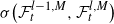 $\sigma\big(\mathcal{F}^{l-1,M}_t,\mathcal{F}^{l,M}_t\big)$
and consider [Reference Jasra, Kamatani, Law and Zhou19, Theorem C.1 and Lemma C.3] under this conditioning. Following the same reasoning as in Remark 4, the constant
 $C(n,\varphi)$
in [Reference Jasra, Kamatani, Law and Zhou19] can be assumed to be deterministic in our setting because the functions a, b,
 $\xi_1$
,
 $\xi_2$
, and G are bounded by Assumptions 1 and 2. Thus, for
 $s\in\{1,2\}$
,
 \begin{equation*} \big|\mathbb{E}\big[\big(\pi^{l,N,M}_{t}(\varphi) - \pi^{l-1,N,M}_{t}(\varphi) - \pi^{l,M}_{t}(\varphi) + \pi^{l-1,M}_{t}(\varphi)\big)^s\big]\big| \leq C\frac{\mathbb{E}[B(n)]^{s/2}}{N},\end{equation*}
where we used the inequality
 $\mathbb{E}[\sqrt{B(n)}]\leq \mathbb{E}[B(n)]^{1/2}$
and B(n) is defined in [Reference Jasra, Kamatani, Law and Zhou19, (C.1)]. Lemma 5.4 verifies an expectation (over all randomness) version of [Reference Jasra, Kamatani, Law and Zhou19, Assumption D.1] from which a version of [Reference Jasra, Kamatani, Law and Zhou19, Theorem D.5] follows (with expectation taken over all randomness). We apply the
 $C^p$
inequality on B(n): the first sum corresponding to maximum coupling is bounded by our version of [Reference Jasra, Kamatani, Law and Zhou19, Theorem D.5], and for the other terms Lemmata 7 and 8 suffice. Therefore, we have
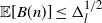 $\mathbb{E}[B(n)]\leq \Delta_l^{1/2}$
. We state the result of this discussion as the following lemma.
Lemma 14. Assume Assumptions 1 and 2. Let
 $\varphi\in\mathcal{C}_\mathrm{b}^1(\mathbb{R}^d)\cap\mathcal{B}_\mathrm{b}(\mathbb{R}^d)$
and
 $t\in\{1,\dots,T\}$
. There exists
 $C<+\infty$
such that, for every
 $(l,N,M)\in\mathbb{N}\times\mathbb{N}\times \mathbb{N}$
and
 $s\in\{1,2\}$
,
 \begin{equation*} \big|\mathbb{E}\big[\big(\pi^{l,N,M}_{t}(\varphi) - \pi^{l-1,N,M}_{t}(\varphi) - \pi^{l,M}_{t}(\varphi) + \pi^{l-1,M}_{t}(\varphi)\big)^s\big]\big| \leq C\frac{\Delta_l^{s/4}}{N}. \end{equation*}
Proof of Theorem 2.
 \begin{align*} & \mathbb{E}\big[\big(\pi_t(\varphi)-\widehat{\pi^L_t(\varphi)}\big)^2\big] \\ & = \mathbb{E}\Bigg[\Bigg(\big(\pi_t(\varphi) - \pi_t^L(\varphi)\big) + \big(\pi_t^{0}(\varphi) - \pi_t^{0,M_0}(\varphi)\big) + \big(\pi_t^{0,M_0}(\varphi) - \pi_t^{0,N_0,M_0}(\varphi)\big) \\ &\kern23pt \quad + \sum_{l=1}^L\big(\pi^{l}_t - \pi^{l-1}_t - \pi^{l,M_l}_t + \pi^{l-1,M_l}_t\big)(\varphi) \\ & \kern23pt\quad + \sum_{l=1}^L\big(\pi^{l,M_l}_t-\pi^{l-1,M_l}_t-\pi^{l,N_l,M_l}_t+\pi^{l-1,N_l,M_l}_t\big) (\varphi)\Bigg)^2\Bigg] \\ & \leq C(\pi_t(\varphi)-\pi_t^L(\varphi))^2 + C\mathbb{E}\big[\big(\pi_t^{0}(\varphi) - \pi_t^{0,M_0}(\varphi)\big)^2\big] \\ & \quad + C\mathbb{E}\Bigg[\Bigg(\sum_{l=1}^L\big(\pi^{l}_t - \pi^{l-1}_t-\pi^{l,M_l}_t +\pi^{l-1,M_l}_t\big) (\varphi)\Bigg)^2\Bigg] + C\mathbb{E}\big[\big(\pi_t^{0,M_0}(\varphi) - \pi_t^{0,N_0,M_0}(\varphi)\big)^2\big] \\ & \quad + C\mathbb{E}\Bigg[\Bigg(\sum_{l=1}^L\big(\pi^{l,M_l}_t - \pi^{l-1,M_l}_t-\pi^{l,N_l,M_l}_t +\pi^{l-1,N_l,M_l}_t\big) (\varphi)\Bigg)^2\Bigg]. \end{align*}
The first term is bounded using
 $C\Delta_L^2$
by Lemma 12; the bounds for the second and third terms follow from the inequality
 $\big(\sum_{i=1}^La_i\big)^2\leq L\sum_{i=1}^La_i^2$
for all
 $a_1,\dots,a_L\in\mathbb{R}$
and Lemma 9. The fourth is the error of a standard particle filter as stated in Lemma 13. For the fifth term we use Lemma 14 as follows:
 \begin{align*} & \mathbb{E}\Bigg[\Bigg(\sum_{l=1}^L\big(\pi_{t}^{l,M_l}-\pi_{t}^{l-1,M_l}-\pi_{t}^{l,N_l,M_l}+\pi_{t}^{l-1,N_l,M_l}\big) (\varphi)\Bigg)^2\Bigg] \\ & \qquad = \sum_{l=1}^L\mathbb{E}\big[\big(\big(\pi_{t}^{l,M_l} - \pi_{t}^{l,M_l} - \pi_{t}^{l-1,N_l,M_l} + \pi_{t}^{l-1,N_l,M_l}\big)(\varphi)\big)^2\big] \\ & \qquad\quad + \sum_{p\not=q}\Big(\mathbb{E}\big[\big(\pi_{t}^{p,M_{p}} - \pi_{t}^{p-1,M_{p}} - \pi_{t}^{p,N_{p},M_{p}} + \pi_{t}^{p-1,N_{p},M_{p}}\big)(\varphi)\big] \\ & \kern32pt\qquad\quad \times \mathbb{E}\big[\big(\pi_{t}^{q,M_{q}} - \pi_{t}^{q-1,M_{q}} - \pi_{t}^{q,N_{q},M_{q}} + \pi_{t}^{q-1,N_{q},M_{q}}\big)(\varphi)\big]\Big) \\ & \qquad \leq C\sum_{l=1}^L\frac{\Delta_l^{1/2}}{N_l} + C\sum_{p\not=q}\frac{\Delta_p^{1/4}\Delta_q^{1/4}}{N_pN_q} \leq C\sum_{l=1}^L\frac{\Delta_l^{1/2}}{N_l}, \end{align*}
where for the last inequality first notice that Assumption 3 implies that
 $N_l\geq (L-l)^2/2$
for
 $0\leq l\leq L-1$
, and then, using the Cauchy–Schwarz inequality,
 \begin{align*} C\sum_{p\not=q}\frac{\Delta_p^{1/4}\Delta_q^{1/4}}{N_pN_q} \leq C\Bigg(\sum_{l=1}^L\frac{\Delta_l^{1/4}}{N_l}\Bigg)^2 & \leq C\Bigg(\sum_{l=1}^L\frac{1}{N_l}\Bigg)\Bigg(\sum_{l=1}^L\frac{\Delta_l^{1/2}}{N_l}\Bigg) \\ & < C\Bigg(1+\frac{1}{2}\sum_{l=1}^{\infty}\frac{1}{l^2}\Bigg)\Bigg(\sum_{l=1}^L\frac{\Delta_l^{1/2}}{N_l}\Bigg). \end{align*}
Funding information
This paper forms part of EA’s PhD thesis at KAUST. AJ was supported by start-up funding at CUHK-SZ.
Competing interests
There were no competing interests to declare which arose during the preparation or publication process of this article.
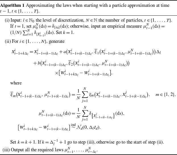
 t−1
 t∈{1,…,T}
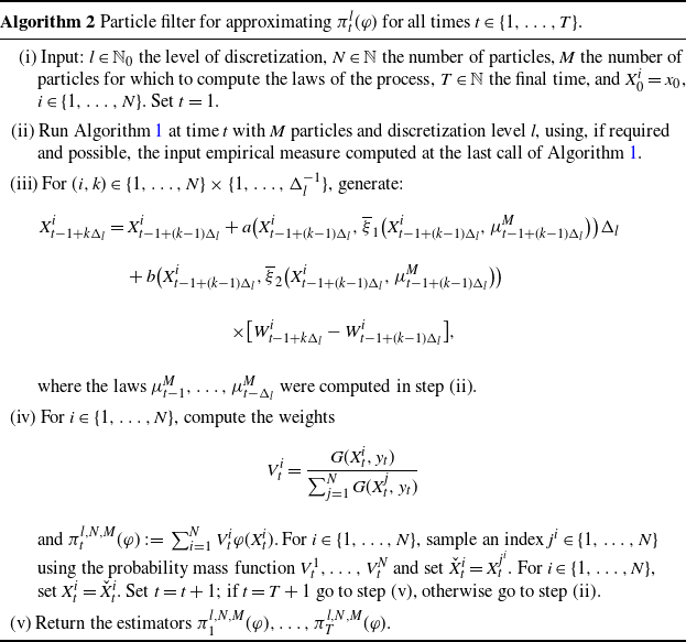
 πtl(φ)
 t∈{1,…,T}
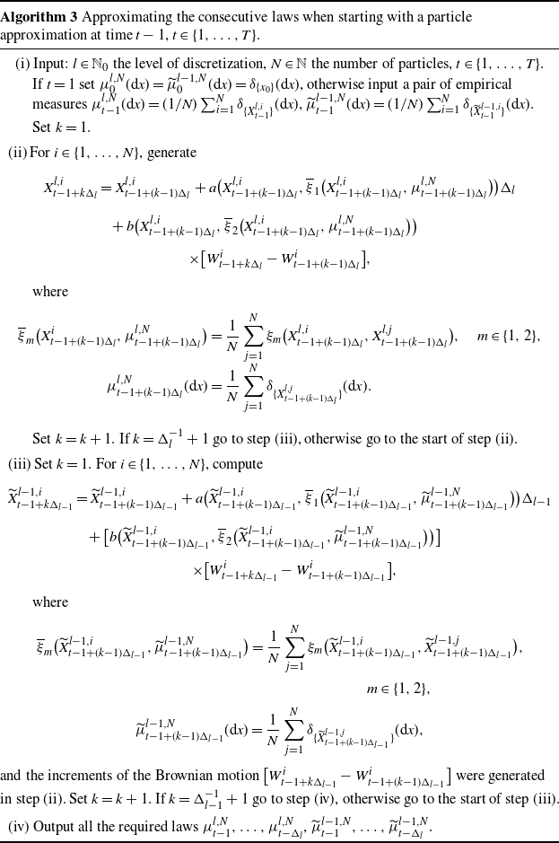
 t−1
 t∈{1,…,T}
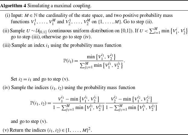
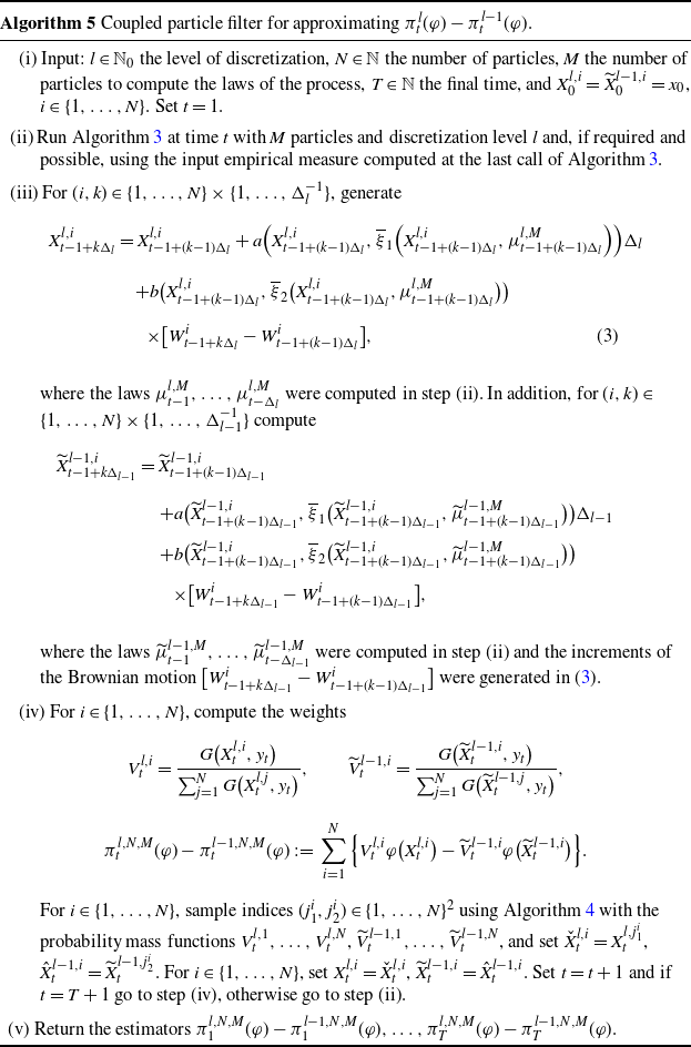
 πtl(φ)−πtl−1(φ)

 2≤L≤6
 3≤L≤6
 2≤L≤6
 3≤L≤6


