1. Introduction
The increments along the diagonal of a loss development triangle correspond to the same calendar year and are therefore subject to common external influences, such as inflation (see, e.g., Clark, Reference Clark2006). These so-called calendar year effects – also referred to as diagonal effects or accounting year effects – pose a persistent challenge in reserving calculations, as they violate the assumption of independence between accident years, a key premise of many reserving models (see, e.g., Wüthrich and Merz, Reference Wüthrich and Merz2008). This paper extends a log-normal chain ladder model that closely aligns with Mack’s assumptions, allowing external market information on calendar year effects to be incorporated in a principled manner into individual reserving calculations.
Several methods have been proposed to identify calendar year effects directly from loss development triangles. Early approaches, such as the separation techniques introduced by Verbeek (Reference Verbeek1972) and Taylor (Reference Taylor1977), often struggle to deliver stable and reliable estimates.
More recently, calendar year effects have been incorporated into generalized linear model (GLM)-based models for incremental losses. Notable contributions include the work of Kuang et al. (Reference Kuang, Nielsen and Nielsen2008a,b, Reference Kuang, Nielsen and Perch Nielsen2011), Kuang and Nielsen (Reference Kuang and Nielsen2020), Brydon and Verrall (Reference Brydon and Verrall2009), and Jessen and Rietdorf (Reference Jessen and Rietdorf2011), who extend Kremer’s log-linear model (see Kremer, Reference Kremer1982) and the over-dispersed Poisson (ODP) model (see Renshaw and Verrall, Reference Renshaw and Verrall1998) to account for diagonal effects.
The ODP model is often referred to as a chain ladder model, since maximum likelihood estimation (MLE) under this model reproduces the classical chain ladder predictions; some even call it the chain ladder model. However, the underlying stochastic assumptions of the ODP model – and of other GLM-based models for incremental losses – differ fundamentally from those of Mack’s chain ladder model, which is defined by the following model assumptions (see Mack, Reference Mack1993).
Mack’s chain ladder model.
-
CL1: The accident years are independent.
-
CL2: There exist parameters
 $m_k\gt0$
such that the cumulative claims
$C_{i,k}$
of accident year i after k development years satisfy
$ \operatorname{E}\!(C_{i,k}|C_{i,1},\dots,C_{i,k-1})=m_kC_{i,k-1}$
.
-
CL3: There exist parameters
$s_k\gt0$
such that
$ \operatorname{Var}\!(C_{i,k}|C_{i,1},\dots,C_{i,k-1})=s^2_kC_{i,k-1}$
.


In contrast to GLMs for incremental losses, which assume independence, Mack’s assumptions imply strong positive dependence among the increments within each accident year. A practical advantage of Mack’s model is its ability to handle negative increments, unlike many GLM-based approaches. For a detailed discussion of the differences in the underlying assumptions, see Mack (Reference Mack1994).
A model that exhibits closer structural similarity to Mack’s model is Hertig’s log-link ratio model (see Hertig, Reference Hertig1985). This model is consistent with the assumptions CL1 and CL2. However, Hertig assumes that the loss development factors (LDFs)
 $C_{i,k}/C_{i,k-1}$
are independent of the loss history
 $C_{i,1},\dots,C_{i,k-1}$
. While this assumption renders the model considerably more tractable than Mack’s formulation, it may be unrealistic in situations where claim volumes vary substantially across accident years.
De Jong (Reference De Jong2006) extends Hertig’s model by incorporating calendar year correlations. Hertig’s framework also forms the basis for the log-normal Bayes chain ladder model proposed by Salzmann and Wüthrich (Reference Salzmann and Wüthrich2012), which also allows for calendar year effects. An extension of the gamma-gamma Bayes chain ladder model that is fully consistent with Mack’s assumptions was introduced by Wüthrich (Reference Wüthrich2010). These Bayes chain ladder models use, among other inputs, prior information on the expected LDFs.
In some cases, external market information on the relative impact of calendar year effects is available. In this paper, we introduce the CLMCLcy model, which extends a log-normal chain ladder framework closely aligned with Mack’s assumptions and allows such information to be incorporated without using prior assumptions on expected LDFs.
This is particularly relevant in practice, since expected LDFs may vary substantially across portfolios within a given market segment, whereas the relative impact of calendar year effects is often similar across triangles. To the best of our knowledge, no extension of Mack’s chain ladder model has been proposed that allows this type of market information to be incorporated.
An example of such market data is provided in Table 1, which shows LDFs for the Other Liability – Occurrence segment from US Schedule P data (Source: S&P Global Market Intelligence). The first diagonal contains LDFs from calendar year 2016 to 2017, while the last diagonal displays those from calendar year 2023 to 2024. In each column, the two smallest development factors are highlighted in gray. A pronounced reduction in development factors is visible from calendar year 2019 to 2020 and again from calendar year 2020 to 2021, attributable to the COVID-19 pandemic.
An extension of the additive claims reserving model that permits the incorporation of prior information on calendar year effects in a Bayesian sense was proposed by Riegel (Reference Riegel2023). This model assumes normally distributed increments, incorporates calendar year effects as latent variables, and employs the expectation-maximization (EM) algorithm (see Dempster et al., Reference Dempster, Laird and Rubin1977) for MLE. Unfortunately, such an additive approach is often not applicable in practice, as it depends on accurate volume measures, which are typically unavailable in industry datasets. In particular, market information structured as in Table 1 cannot be used directly.
To enable a similar extension of Mack’s chain ladder model (that does not need volumes), a natural starting point is to augment the model by assuming that the LDFs are conditionally log-normally distributed. Taking logarithms of the LDFs then yields an additive structure with normally distributed variables. However, this approach gives rise to two challenges:
-
• In such a parametric variant of Mack’s model, MLE requires numerical optimization (see Riegel, Reference Riegel2026).
-
• In contrast to the additive model, the resulting normally distributed variables are no longer independent.
To address the first challenge, we adopt the log-normal Mack chain ladder (LMCL) model proposed by Riegel (Reference Riegel2026) as the basis for our extension. This model is specifically designed to align closely with Mack’s assumptions while allowing for MLE via an iterative algorithm. In this model, logarithmic transformation of the LDFs yields a structure that can be treated using the EM algorithm in a similar way as in the additive case of Riegel (Reference Riegel2023), even though the dependence structure and the need for iterative MLE in the LMCL model introduce additional complexity.
Loss development factors
 $L_{i,k}^{\operatorname{OL\,Occ}}$
for cumulative payments in the segment Other Liability – Occurrence (industry excluding outliers). In each column, the two smallest LDFs are highlighted in gray.

Table 1 Long description
A table titled ‘LDF L subscript i,k superscript OL Occ from development year k - 1 to k for occurrence year i’ presents loss development factors for cumulative payments in the Other Liability Occurrence segment. The table has 12 rows and 9 columns. The rows are labeled with occurrence years from 2009 to 2023. The columns are labeled with development years k ranging from 2 to 10. Each cell contains a numerical value representing the loss development factor for the corresponding occurrence and development years. The two smallest LDFs in each column are highlighted in gray. The table shows the following data: Row 2009: k = 2, 1.039; k = 3, 1.028. Row 2010: k = 2, 1.069; k = 3, 1.034; k = 4, 1.019. Row 2011: k = 2, 1.087; k = 3, 1.058; k = 4, 1.032; k = 5, 1.022. Row 2012: k = 2, 1.185; k = 3, 1.078; k = 4, 1.050; k = 5, 1.024; k = 6, 1.017. Row 2013: k = 2, 1.287; k = 3, 1.130; k = 4, 1.078; k = 5, 1.064; k = 6, 1.033; k = 7, 1.021. Row 2014: k = 2, 1.489; k = 3, 1.229; k = 4, 1.134; k = 5, 1.064; k = 6, 1.033; k = 7, 1.021. Row 2015: k = 2, 1.813; k = 3, 1.451; k = 4, 1.242; k = 5, 1.113; k = 6, 1.056; k = 7, 1.043; k = 8, 1.040; k = 9, 1.029. Row 2016: k = 2, 2.720; k = 3, 1.757; k = 4, 1.440; k = 5, 1.204; k = 6, 1.111; k = 7, 1.106; k = 8, 1.066; k = 9, 1.043. Row 2017: k = 2, 2.824; k = 3, 1.706; k = 4, 1.408; k = 5, 1.213; k = 6, 1.172; k = 7, 1.129; k = 8, 1.061. Row 2018: k = 2, 2.829; k = 3, 1.628; k = 4, 1.351; k = 5, 1.279; k = 6, 1.193; k = 7, 1.104. Row 2019: k = 2, 2.422; k = 3, 1.599; k = 4, 1.476; k = 5, 1.278; k = 6, 1.164. Row 2020: k = 2, 2.328; k = 3, 1.698; k = 4, 1.431; k = 5, 1.271. Row 2021: k = 2, 2.840; k = 3, 1.720; k = 4, 1.478. Row 2022: k = 2, 2.725; k = 3, 1.742. Row 2023: k = 2, 2.691.
Organization of the paper: In Section 2, we extend the LMCL model by introducing latent variables to capture calendar year effects. Section 3 presents a version of the EM algorithm for computing maximum likelihood estimates of the parameters and posterior means of the calendar year effects. Standard error estimates for the resulting reserving method are derived in Section 4. Unlike in Mack’s chain ladder model, the variance parameter estimates influence the prediction of future claim development, which may lead to instability. To address this, Section 5 adopts a robustification approach similar to that in Riegel (Reference Riegel2025). A case study based on the Schedule P data from Table 1, along with a detailed performance analysis, is provided in the online supplementary material. Some technical calculations have been moved to the appendix.
2. A log-normal chain ladder model with calendar year effects
For
 $i\in \{1,\dots, m\}$
and
 $k\in \{1,\dots, n\}$
let
 $C_{i,k}\gt0$
denote the cumulative claims of accident year i after development year k (payments or incurred amounts). Then
 $C_{i,k}$
is the cumulative claims amount of the accident year i after the calendar year
 $i+k-1$
. We assume that the random variables
 $C_{i,k}$
are observable up to the calendar year p (i.e., for
 $i+k\le p+1$
) for a p with
 $\max (m,n)\le p \lt m+n-1$
. Let
 ${A}\, :\!= \,\{1,\dots,m\}\times\{1,\dots,n\}$
denote the set of all pairs of accident and development years and let
 $\mathcal{O}\, :\!= \,\{(i,k)\in\mathcal{A}\,|\, i+k\le p+1\}$
be the subset containing the indices of the observable
 $C_{i,k}$
. The set of indices corresponding to calendar year q is denoted by
 $\mathcal{C}(q)\, :\!= \,\{(i,k)\in \mathcal{A}\,|\, i+k=q+1\}$
. The purpose of a reserving method is to predict the cumulative amounts
 $C_{i,k}$
with
 $(i,k)\in \mathcal{P}\, :\!= \,\mathcal{A}\setminus\mathcal{O}$
. We define
 \begin{align*}I(k)\, :\!= \,\min\{p-k+1,m\}\quad\text{and}\quad K(i)\, :\!= \,\min\{p-i+1,n\} \end{align*}
such that
 $C_{1,k},\dots,C_{I(k),k}$
are the observable cumulative claims with development year k and
 $C_{i,1},\dots,C_{i,K(i)}$
are the observable cumulative claims from accident year i. The LDFs
 \begin{align*}R_{i,k}\, :\!= \,\frac{C_{i,k}}{C_{i,k-1}} \end{align*}
are defined for
 $(i,k)\in \mathcal{A}^*\, :\!= \,\{(i,k)\in \mathcal{A}\,|\, i\ge 2\}$
and observable for
 $(i,k)\in \mathcal{O}^*\, :\!= \,\mathcal{O}\cap \mathcal{A}^*$
. The developments of calendar year q are described by the LDFs
 $R_{i,k}$
with indices
 $(i,k)\in \mathcal{C}^*(q)\, :\!= \,\mathcal{C}(q)\cap \mathcal{A}^*$
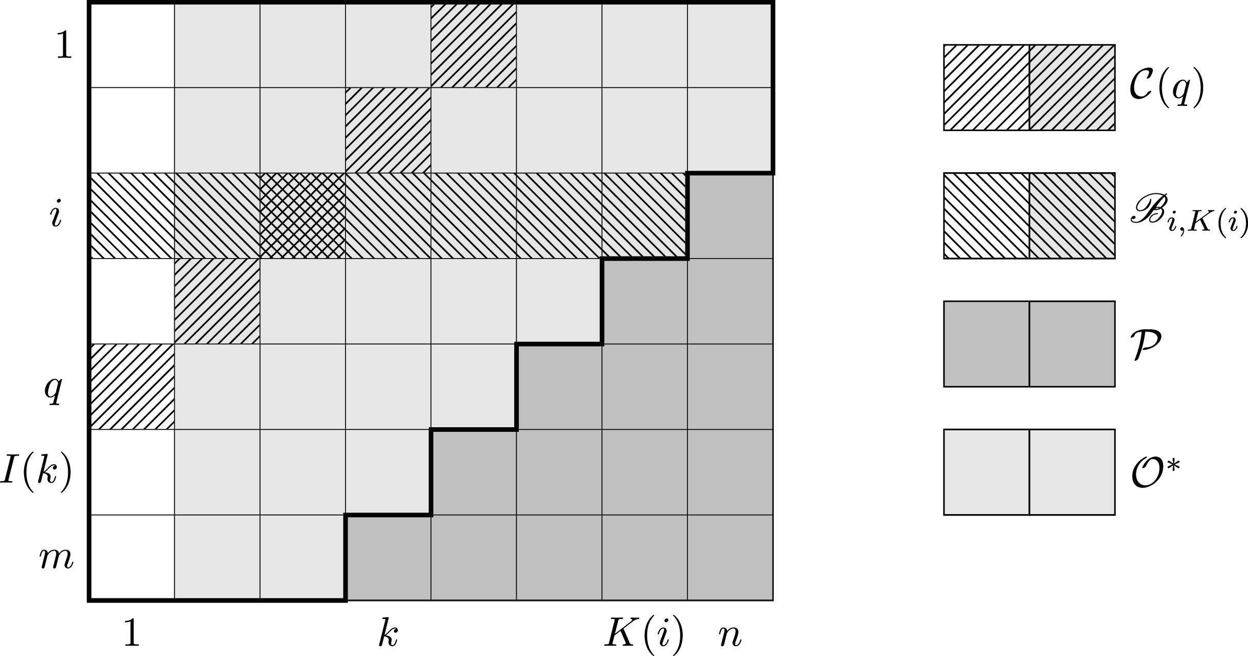
. This notation is illustrated in Figure 1.
Illustration of the notation.

For simplicity, we assume that the random variables
 $C_{1,1},\dots,C_{m,1}$
are deterministic. Alternatively, the entire analysis could be performed conditionally, given
 $C_{1,1},\dots,C_{m,1}$
. Let
 \begin{align*}\mathscr{B}_{i,k}\, :\!= \,\sigma(C_{i,1},\dots,C_{i,k}) \end{align*}
be the sigma algebra generated by
 $C_{i,1},\dots,C_{i,k}$
and let
 $\operatorname{P}^{X|\mathscr{B}}$
denote the conditional distribution of a random variable X given a
 $\sigma$
-algebra
 $\mathscr{B}$
.
The following two model assumptions define the LMCL model (see Riegel, Reference Riegel2026), which will be used as basis for our study. By design, the LMCL model adheres closely to Mack’s chain ladder assumptions. In particular, its variance assumptions are considerably more in line with Mack’s framework than those of Hertig’s model. Below, we will extend the model assumptions to consider calendar year effects.
Log-normal Mack chain ladder (LMCL) model.
-
LMCL1: The accident years are independent.
-
LMCL2: There are parameters
$\mu_2,\dots,\mu_{n}$
and
$\sigma_2,\dots, \sigma_{n}\gt0$
such that
\begin{align*} \operatorname{P}^{R_{i,k}|\mathscr{B}_{i,k-1}} = \operatorname{LogNormal}\!(\mu_{k}-\sigma^2_k/(2C_{i,k-1}),\sigma^2_k/C_{i,k-1}). \end{align*}


With
 $m_k\, :\!= \,\exp\!(\mu_k)$
and
 $s_k\, :\!= \,m_k\sigma_k$
assumption LMCL2 implies
 \begin{equation}\operatorname{E}\!(R_{i,k}|\mathscr{B}_{i,k-1})=\exp\!(\mu_k)=m_k \end{equation}
and
 \begin{equation}\operatorname{Var}\!(R_{i,k}|\mathscr{B}_{i,k-1})=\exp\!(\mu_k)^2\cdot\left[\exp\!\left(\frac{\sigma_k^2}{C_{i,k-1}}\right)-1\right]\approx \exp\!(\mu_k)^2\cdot \frac{\sigma_k^2}{C_{i,k-1}}=\frac{s_k^2}{C_{i,k-1}}, \end{equation}
where we have used the linear approximation
 $\exp\!(x)-1\approx \exp\!(0)+\exp'(0)x-1=x$
in (2). Consequently, the LMCL model satisfies the chain ladder assumptions CL1 and CL2 and satisfies CL3 approximately.
Riegel (Reference Riegel2026) proposes an iteration for computing maximum likelihood estimators of the parameters
 $\mu_2,\dots, \mu_n$
and
 $\sigma_2,\dots,\sigma_n$
, and uses them to introduce a new reserving method, referred to as the the LMCL method. The paper also discusses the accuracy of the underlying approximation and presents several numerical examples demonstrating that the LMCL method is closely aligned with the chain ladder method.
In the following, we introduce the LMCLcy model, which extends the LMCL model by incorporating calendar year effects. For
 $(i,k)\in \mathcal{A}^*$
, we model the calendar year effects with log-normally distributed random variables
 $F_{i,k}$
, which scale the LDFs
 $R_{i,j}$
. The moments
 \begin{align*}f_{i,k}\, :\!= \,\operatorname{E}\!(F_{i,k})\gt0\quad \text{and}\quad t_{i,k}^2\, :\!= \,\operatorname{Var}\!(F_{i,k})\gt0 \end{align*}
are provided as prior information.
 $f_{i,k}$
represents the average impact of a calendar year effect in the market, whereas
 $t_{i,k}$
reflects the degree to which this effect varies across portfolios. A small value of
 $t_{i,k}$
indicates that all portfolios are affected in a similar way, whereas a large value suggests substantial heterogeneity.
For calendar years q in which no exceptional market-wide effects on the LDFs are observed, the intention is to set
 $f_{i,k}=1$
for all
 $(i,k)\in \mathcal{C}^*(q)$
. Note that
 $f_{i,k}=1$
for all
 $(i,k)\in \mathcal{A}^*$
does not imply the absence of calendar year effects; for instance, constant calendar year inflation does not distort the LDFs in a triangle. The factors
 $F_{i,k}$
within a fixed calendar year q may differ in their moments; however, since they are intended to model a common calendar year effect, they are assumed to be comonotonic. Calendar year factors belonging to different calendar years are assumed to be independent.
Remark 1. The model assumptions LMCLcy1 and LMCLcy2 below ensure that the moments
 $f_{i,k}$
and
 $t_{i,k}^2$
determine a prior distribution for
 $(F_{i,k})_{(i,k)\in \mathcal{A}^*}$
in the Bayesian sense. Below, we also allow to specify
 $t_{i,k}=0$
. This can be interpreted as limiting case
 $t_{i,k}\to 0$
or simply as
 $t_{i,k}\, :\!= \,\varepsilon$
with a sufficiently small
 $\varepsilon \gt 0$
. In the algorithms for parameter estimation described in Sections 3 and 5, as well as in the mean squared error of prediction (MSEP) estimators, one can directly use the formulas with
 $t_{i,k}=0$
.
Remark 2. If a calendar year effect is expected to persist in the future (“the new normal”), then this can be reflected in the model by setting
 $f_{i,k}\neq 1$
for future years, that is, for
 $(i,k)\in \mathcal{P}$
.
Remark 3. In the case study in the online supplementary material, we estimate the means
 $f_{i,k}$
from the market-wide LDFs provided in Table 1. If LDFs are available for all (or at least many) portfolios in the market, it may also be possible to estimate the variances
 $t_{i,k}^2$
directly from the data. However, in practice, a pragmatic approach is typically required to specify reasonable values for
 $t_{i,k}$
.
In the case study, we set
 $f_{i,k}=1$
for all normal calendar years, that is, all years which are not systematically affected by COVID-19. In such a situation, one possible approach is to choose a parameter
 $\rho \ge 0$
and define
 \begin{align*} t_{i,k}\, :\!= \,\rho\cdot |f_{i,k}-1|. \end{align*}
The choice
 $\rho=0$
corresponds to the assumption that the calendar year effects observed in the market fully apply to the individual triangle under consideration. As
 $\rho$
increases, less credibility is assigned to the market prior along calendar year diagonals. Note that this approach permits calendar year effects in the individual triangle only in those years, where market-wide effects were observed, that is, for calendar years q for which
 $f_{i,k}\neq 1$
for some
 $(i,k)\in \mathcal{C}^*(q)$
. Strategies for selecting the parameter
 $\rho$
are discussed in the online supplementary material.
An alternative method for selecting the parameters
 $f_{i,k}$
and
 $t_{i,k}^2$
, which is more closely aligned with the approach taken in Riegel (Reference Riegel2023), is provided in Appendix A.
Remark 4. At first glance, one might expect to obtain a non-informative prior as
 $t_{i,k}\to \infty$
. However, this is not the case because we assume log-normal distributions for the
 $F_{i,k}$
. As
 $t_{i,k}$
increases, the distribution of
 $F_{i,k}$
becomes increasingly skewed, with a pronounced mode that approaches zero. This behavior can lead to unexpected effects. As long as
 \begin{align*} \frac{t_{i,k}}{f_{i,k}}=\operatorname{CV}\!(F_{i,k})\le 0.2, \end{align*}
the log-normal density remains close in shape to a normal density with the same first two moments, and no issues arise. In contrast, cases with large coefficients of variation (e.g.,
 $t_{i,k}/f_{i,k}\ge 0.5$
) require careful handling.
Remark 5. In the model assumptions, it is convenient to use the moments
 \begin{align*}\varphi_{i,k}\, :\!= \,\operatorname{E}\!(\!\log(F_{i,k}))\quad \text{and}\quad \tau^2_{i,k}\, :\!= \,\operatorname{Var}\!(\!\log(F_{i,k})) \end{align*}
of the logarithmized calendar year factors
 $\log(F_{i,k})$
– that is, the parameters of the log-normal distributions – instead of the moments
 $f_{i,k}$
and
 $t_{i,k}^2$
. The parameters
 $\varphi_{i,k}$
and
 $\tau_{i,k}^2$
can be calculated from
 $f_{i,k}$
and
 $t_{i,k}^2$
with the formulas
 \begin{align*} \tau_{i,k}^2=\log\left(t_{i,k}^2/f_{i,k}^2+1\right)\quad\text{and}\quad \varphi_{i,k}=\log(f_{i,k})-\tau_{i,k}^2/2. \end{align*}
Vice versa, we have
 \begin{align*}f_{i,k}=\exp\!(\varphi_{i,k}+\tau_{i,k}^2/2)\quad\text{and}\quad t_{i,k}^2=f_{i,k}^2\cdot (\!\exp\!(\tau_{i,k}^2)-1). \end{align*}
Let
 $\mathscr{F}_q$
denote the sigma algebra generated by
 $\{F_{i,k}\,|\,(i,k)\in \mathcal{C}^*(q)\}$
. Straightforward generalization of the model assumptions LMCL1 and LMCL2 leads to the following model.
Log-normal Mack chain ladder model with calendar year effects (LMCLcy model).
-
LMCLcy1: The calendar year factors of different calendar years are independent, that is, the
$\sigma$
-algebras
$\mathscr{F}_2,\dots,\mathscr{F}_{m+n-1}$
are independent. For every calendar year
$q=2,\dots,m+n-1$
the vectoris comonotonic. Conditionally, given
\begin{align*}(F_{i,k})_{(i,k)\in\mathcal{C}^*(q)} \end{align*}
$\mathscr{F}\, :\!= \,\sigma(\mathscr{F}_2,\dots,\mathscr{F}_{m+n-1})$
, the accident years are independent, that is, the vectors are conditionally independent.
\begin{align*} \{(C_{i,1},\dots, C_{i,n})\, |\, i=1,\dots,m\} \end{align*}
-
LMCLcy2: There are known parameters
$\varphi_{i,k}, \tau_{i,k}$
,
$(i,k)\in \mathcal{A}^*$
, such that (prior distribution of the calendar year factors).
\begin{align*} F_{i,k}\sim \operatorname{LogNormal}\!(\varphi_{i,k}, \tau^2_{i,k}) \end{align*}
-
LMCLcy3: There are parameters
$\mu_2,\dots,\mu_{n}$
and
$\sigma_2,\dots, \sigma_{n}\gt0$
such that or equivalently
\begin{align*} \operatorname{P}^{R_{i,k}|\sigma(\mathscr{B}_{i,k-1}, \mathscr{F})} = \operatorname{LogNormal}\!(\mu_{k}-\sigma^2_k/(2C_{i,k-1}) + \log(F_{i,k}),\sigma^2_k/C_{i,k-1}) \end{align*}
\begin{align*} \operatorname{P}^{R_{i,k}/F_{i,k}|\sigma(\mathscr{B}_{i,k-1}, \mathscr{F})} = \operatorname{LogNormal}\!(\mu_{k}-\sigma^2_k/(2C_{i,k-1}) ,\sigma^2_k/C_{i,k-1}). \end{align*}


For the remainder of this paper, we work in this LMCLcy model.
Remark 6. As a consequence of the model assumptions LMCLcy1 and LMCLcy2, there are independent standard normally distributed random variables
 $X_q$
,
 $q\in \{2,\dots,m+n-1\}$
, such that
 \begin{align*} \log(F_{i,k})=\varphi_{i,k}+\tau_{i,k}X_{i+k-1} \end{align*}
for all
 $(i,k)\in \mathcal{A}^*$
. We refer to the
 $X_q$
as residual calendar year effects. Note that the
 $\sigma$
-algebra
 $\mathscr{F}_q$
is generated by
 $X_q$
.
Remark 7. If
 $f_{i,k}= 1$
and
 $t^2_{i,k}\to 0$
for all
 $(i,k)\in\mathcal{A}^*$
, then we obtain the model assumptions of the LMCL model.
3. Parameter estimation and reserving method
The goal of this section is to describe in detail an algorithm to calculate maximum likelihood estimators for the parameters
 $\mu_k$
and
 $\sigma_k$
of the LMCLcy model and the posterior distribution of the calendar year factors
 $F_{i,k}$
. Like in Riegel (Reference Riegel2023), we employ the EM algorithm, see Dempster et al. (Reference Dempster, Laird and Rubin1977). We assume
 $p\gt n$
to avoid problems with the estimation of
 $\sigma_n$
. A pragmatic solution for the case
 $p=n$
is provided in Remark 8.
The resulting estimators for
 $\mu_k$
and
 $\sigma_k$
can be used to predict the future claim development, leading to the LMCLcy method. This method suffers from the problem that many parameters have to be estimated. In particular, the estimation of individual variance parameters
 $\sigma_k$
for each development year k can lead to instabilities and unexpected results. In Section 5, we describe a robustified variant of the method, which is recommended for application in practice.
Let
 $T_{i,k}\, :\!= \,\log(R_{i,k})$
. We consider the vector
 $T\, :\!= \,(T_{i,k})_{(i,k)\in \mathcal{O}^*}$
consisting of the logarithmized observable LDFs and the vector
 $X\, :\!= \,(X_2,\dots,X_p)$
containing the residual calendar year effects of the observable calendar years (see Remark 6). Note that X is not observable. Let
 $\Theta \, :\!= \,(\mu,\sigma)\, :\!= \,(\mu_2,\dots, \mu_n, \sigma_2,\dots, \sigma_n)$
. The density
 $p_{(X,T)}(\cdot\, ;\Theta)$
of (X, T) has a relatively simple form:
 \begin{align*} p_{(X, T)} (x, t;\, \Theta) & =p_{(X, T)} ((x_q)_{q=2,\dots,p}, (t_{i,k})_{(i,k)\in \mathcal{O}^*};\, \Theta) \\[3pt] &=\prod_{q=2}^{p}\frac{1}{\sqrt {2\pi}}\exp\left(-\frac{x_q^2}{2} \right) \\[3pt] &\phantom{aaaaaa}\cdot\prod_{(i,k)\in \mathcal{O}^*}\frac{1}{\sqrt {2\pi \sigma_k^2/C_{i,k-1}}}\exp\left(-\frac{[t_{i,k}-( \mu_k-\sigma^2_k/(2C_{i,k-1}) + \varphi_{i,k} +\tau_{i,k}x_{i+k-1})]^2}{2\sigma_k^2/C_{i,k-1}} \right)\!.\end{align*}
In order to calculate the maximum likelihood estimators, we have to maximize the log-likelihood of the observable data T:
 \begin{align*}\ell_T(\Theta)=\log p_T(T; \Theta)=\log \int_{\mathbb{R}^{p-1}}p_{(X, T)} (x, T;\, \Theta)\, \, dx. \end{align*}
Unfortunately,
 $\ell_T$
is not as simple as the log-likelihood
 $\ell_{(X,T)}(\Theta)=\log(p_{(X, T)}(X,T;\,\Theta))$
of the complete data (X, T). The EM algorithm is an iterative method to find (local) maxima of the observable log-likelihood in such a situation.
The EM iteration alternates between performing an expectation step (E step), which calculates the expected log-likelihood function using the current estimate for the parameters, and a maximization step (M step), which computes new parameters maximizing the expected log-likelihood found in the E step. These parameter estimates are then used to determine the conditional distribution of the latent variables and the expected log-likelihood function in the next E step. In our case, we define
 \begin{align*}Q(\Theta|\Theta')\, :\!= \,\operatorname{E}_{X|T;\,\Theta'}\Big(\!\log\big(p_{(X,T)}(X,T;\,\Theta)\big)\Big) \end{align*}
and start with an initial parameter vector
 $\widehat{\Theta}^{(0)}$
. Given
 $\widehat{\Theta}^{\,(\nu)}$
, we calculate
 $Q(\Theta|\widehat{\Theta}^{\,(\nu)})$
in the E step and in the M step we choose
 $\widehat{\Theta}^{\,(\nu+1)}$
to be any value which maximizes
 $Q(\cdot\,|\widehat{\Theta}^{\,(\nu)})$
.
The following proposition provides the conditional distribution of the latent variables X, given T and
 $\Theta$
, which is needed in the calculation of the expected log-likelihood in the E step. We define the functions
 $a_q\colon \mathbb{R}^{n-1}\times (0,\infty)^{n-1} \to \mathbb{R}$
and
 $b_q\colon \mathbb{R}^{n-1}\times(0,\infty)^{n-1} \to \mathbb{R}$
,
 $q=2,\dots,p$
, by
 \begin{align*}a_q(\mu,\sigma)\, :\!= \, \left(1 + \sum_{(i,k)\in \mathcal{C}^*(q)} \frac{ \tau_{i,k}^2}{\sigma_k^2/C_{i,k-1}}\right)^{-1} \end{align*}
and
 \begin{align*}b_q(\mu,\sigma) \, :\!= \, a_q(\mu,\sigma)\cdot\sum_{(i,k)\in \mathcal{C}^*(q)}\left(\frac{T_{i,k} -(\mu_k+\varphi_{i,k})}{\sigma_k^2/C_{i,k-1}}+\frac{1}{2}\right)\cdot \tau_{i,k}. \end{align*}
Proposition 1. Conditionally, given T and a parameter vector
 $\Theta$
, the vector X is normally distributed with mean
 $b(\Theta)$
and covariance matrix
 $\Sigma(\Theta)$
, where
 \begin{align*} b(\Theta)\, :\!= \,\left(\begin{array}{ccc} b_2(\Theta) \\[3pt] \vdots \\[3pt] b_p(\Theta), \end{array} \right) \quad \text{ and }\quad \Sigma(\Theta)\, :\!= \,\left( \begin{array}{ccc} a_2(\Theta) & & 0 \\[3pt] &\quad \ddots &\quad \\[3pt] 0 &\quad &\quad a_p(\Theta) \end{array} \right). \end{align*}
Proof. For
 $q=2,\dots,p$
, we have
 \begin{align*} \frac{x_q^2}{2} & + \sum_{(i,k)\in\mathcal{C}^*(q)} \frac{[T_{i,k}-( \mu_k -\sigma^2_k/(2C_{i,k-1})+ \varphi_{i,k} +\tau_{i,k}x_{i+k-1})]^2}{2\sigma_k^2/C_{i,k-1}} \\[3pt] & = \frac{x_q^2}{2} + \sum_{(i,k)\in\mathcal{C}^*(q)} \frac{ ( \mu_k-\sigma^2_k/(2C_{i,k-1}) + \varphi_{i,k} +\tau_{i,k}x_{q})^2}{2\sigma_k^2/C_{i,k-1}} \\[3pt] & \qquad\,\, - \sum_{(i,k)\in\mathcal{C}^*(q)} \frac{2 T_{i,k}( \mu_k -\sigma^2_k/(2C_{i,k-1})+ \varphi_{i,k} +\tau_{i,k}x_{q})}{2\sigma_k^2/C_{i,k-1}} + \sum_{(i,k)\in\mathcal{C}^*(q)} \frac{T_{i,k}^2}{2\sigma_k^2/C_{i,k-1}} \\[3pt] & = \frac{1}{2}\left(1 + \sum_{(i,k)\in\mathcal{C}^*(q)} \frac{ \tau_{i,k}^2}{\sigma_k^2/C_{i,k-1}} \right) x_q^2 - \left(\sum_{(i,k)\in\mathcal{C}^*(q)} \frac{ T_{i,k} \tau_{i,k}-(\mu_k-\sigma^2_k/(2C_{i,k-1})+\varphi_{i,k})\tau_{i,k}}{\sigma_k^2/C_{i,k-1}} \right)x_q + c_1 \\[3pt] & = \frac{1}{2}a_q(\Theta)^{-1} x_q^2 - a_q(\Theta)^{-1}b_q(\Theta) x_q + c_1 \\[3pt] & =\frac{1}{2}a_q(\Theta)^{-1}(x_q-b_q(\Theta))^2 + c_2\end{align*}
with constants
 $c_1,c_2$
that do not depend on
 $(x_2,\dots, x_p)$
. Consequently, we have
 \begin{align*}p_{X|T;\,\Theta}(x)\propto \prod_{q=2}^p \exp\left(-\frac{1}{2}a_q(\Theta)^{-1}(x_q-b_q(\Theta))^2\right)\!. \end{align*}
We define
 \begin{align*}c_{i,k}(\Theta)\, :\!= \,\tau_{i,k}^2\cdot a_{i+k-1}(\Theta),\qquad d_{i,k}(\Theta)\, :\!= \,\varphi_{i,k}+\tau_{i,k}b_{i+k-1}(\Theta) \end{align*}
and
 $G_{i,k}\, :\!= \,\log(F_{i,k})=\varphi_{i,k}+ \tau_{i,k}X_{i+k-1}$
. Then,
 $\operatorname{E}\!(G_{i,k}\,|\,T;\,\Theta)=d_{i,k}(\Theta)$
and
 $\operatorname{Var}\!(G_{i,k}\,|\,T;\,\Theta)=c_{i,k}(\Theta)$
. Given an estimate
 $\widehat{\Theta}^{\,(\nu)}$
, we can use Proposition 1 to perform the E step:
 \begin{align*} Q(\Theta & |\widehat{\Theta}^{\,(\nu)}) = \\[3pt] &=\operatorname{E}_{X|T;\,\widehat{\Theta}^{\,(\nu)}}\big(\!\log \big(p_{(X,T)}(X,T;\,\Theta)\big)\big) \\[3pt] & = \operatorname{E}_{X|T;\,\widehat{\Theta}^{\,(\nu)}} \left(\sum_{q=2}^{p} \left(- \frac{X_q^2}{2} \right)\right)+ \sum_{(i,k)\in \mathcal{O}^*}\left(-\log(\sigma_k)\right) \\[3pt] & \phantom{aaaa} + \operatorname{E}_{X|T;\,\widehat{\Theta}^{\,(\nu)}} \left(\sum_{(i,k)\in\mathcal{O}^*}\left(-\frac{[G_{i,k} - (T_{i,k}- \mu_k+\sigma^2_k/(2C_{i,k-1}))]^2}{2\sigma_k^2/C_{i,k-1}} \right) \right) +c\\[3pt] & = \operatorname{E}_{X|T;\,\widehat{\Theta}^{\,(\nu)}} \left(\sum_{q=2}^{p} \left(- \frac{X_q^2}{2} \right)\right)+ \sum_{(i,k)\in \mathcal{O}^*}\left(-\log(\sigma_k)\right) - \operatorname{E}_{X|T;\,\widehat{\Theta}^{\,(\nu)}} \left(\sum_{(i,k)\in\mathcal{O}^*}\left(\frac{G_{i,k}^2 }{2\sigma_k^2/C_{i,k-1}} \right) \right)\\[3pt] & \phantom{aaaa} + \operatorname{E}_{X|T;\,\widehat{\Theta}^{\,(\nu)}} \left(\sum_{(i,k)\in\mathcal{O}^*}\left(\frac{2G_{i,k}(T_{i,k}- \mu_k+\sigma^2_k/(2C_{i,k-1}))}{2\sigma_k^2/C_{i,k-1}} \right) \right)\\[3pt] & \phantom{aaaa} - \operatorname{E}_{X|T;\,\widehat{\Theta}^{\,(\nu)}} \left(\sum_{(i,k)\in\mathcal{O}^*}\left(\frac{(T_{i,k}- \mu_k+\sigma^2_k/(2C_{i,k-1}))^2}{2\sigma_k^2/C_{i,k-1}} \right) \right) +c\end{align*}
 \begin{align*} & = \sum_{q=2}^{p} \left( - \frac{a_q(\widehat{\Theta}^{\,(\nu)}) + b_q(\widehat{\Theta}^{\,(\nu)})^2}{2} \right) - \sum_{(i,k)\in \mathcal{O}^*}\log(\sigma_k) - \sum_{(i,k)\in \mathcal{O}^*} \left(\frac{c_{i,k}(\widehat{\Theta}^{\,(\nu)})+d_{i,k}(\widehat{\Theta}^{\,(\nu)})^2 }{2\sigma_k^2/C_{i,k-1}} \right)\\[3pt] & \phantom{aaaa} + \sum_{(i,k)\in \mathcal{O}^*} \left(\frac{2d_{i,k}(\widehat{\Theta}^{\,(\nu)})(T_{i,k}-\mu_k+\sigma^2_k/(2C_{i,k-1})) }{2\sigma_k^2/C_{i,k-1}} \right)\\[3pt] & \phantom{aaaa} - \sum_{(i,k)\in \mathcal{O}^*} \left(\frac{ (T_{i,k}-\mu_k+\sigma^2_k/(2C_{i,k-1}))^2}{2\sigma_k^2/C_{i,k-1}} \right) +c \\[3pt] & = \sum_{q=2}^{p} \left( - \frac{a_q(\widehat{\Theta}^{\,(\nu)}) + b_q(\widehat{\Theta}^{\,(\nu)})^2}{2} \right) - \sum_{(i,k)\in \mathcal{O}^*}\log(\sigma_k) \\[3pt] & \phantom{aaaa}- \sum_{(i,k)\in \mathcal{O}^*} \frac{c_{i,k}(\widehat{\Theta}^{\,(\nu)})+d_{i,k}(\widehat{\Theta}^{\,(\nu)})^2 -2d_{i,k}(\widehat{\Theta}^{\,(\nu)})(T_{i,k}-\mu_k) + (T_{i,k}-\mu_k)^2 }{2\sigma_k^2/C_{i,k-1}} \\[3pt] & \phantom{aaaa} -\frac{1}{2} \sum_{(i,k)\in \mathcal{O}^*} \left(T_{i,k}-\mu_k- d_{i,k}(\widehat{\Theta}^{\,(\nu)}) \right)-\frac{1}{8} \sum_{(i,k)\in \mathcal{O}^*} \sigma_k^2/C_{i,k-1} +c\end{align*}
with a constant c. In the M step, we have to solve the following equations for
 $\Theta$
to obtain
 $\widehat{\Theta}^{\,(\nu+1)}$
:
 \begin{align*} 0 & = \frac{\partial}{\partial \mu_k}Q(\Theta|\widehat{\Theta}^{\,(\nu)}) =\sum_{i=1}^{I(k)}\left( - \frac{d_{i,k}(\widehat{\Theta}^{\,(\nu)})+\mu_k-T_{i,k}}{\sigma_k^2/C_{i,k-1}}+\frac{1}{2}\right) \\[3pt] & =\sum_{i=1}^{I(k)}\left(-\frac{C_{i,k-1}\mu_k}{\sigma_k^2} +\frac{C_{i,k-1}(T_{i,k}-d_{i,k}(\widehat{\Theta}^{\,(\nu)}))}{\sigma_k^2}+\frac{1}{2}\right), \\[3pt] 0 & = \frac{\partial}{\partial \sigma_k}Q(\Theta|\widehat{\Theta}^{\,(\nu)}) =\\[3pt] & =-\sum_{i=1}^{I(k)}\frac{1}{\sigma_k}+\sum_{i=1}^{I(k)} \frac{c_{i,k}(\widehat{\Theta}^{\,(\nu)})+d_{i,k}(\widehat{\Theta}^{\,(\nu)})^2 -2d_{i,k}(\widehat{\Theta}^{\,(\nu)})(T_{i,k}-\mu_k) + (T_{i,k}-\mu_k)^2 }{\sigma_k^3/C_{i,k-1}} \\[3pt] & \quad -\frac{1}{4} \sum_{i=1}^{I(k)} \sigma_k/C_{i,k-1} \\[3pt] & = -\frac{I(k)}{\sigma_k}+\sum_{i=1}^{I(k)} \frac{C_{i,k-1}\Big[c_{i,k}(\widehat{\Theta}^{\,(\nu)})+[ T_{i,k}-\mu_k- d_{i,k}(\widehat{\Theta}^{\,(\nu)})]^2\Big] }{\sigma_k^3}- \sigma_k\sum_{i=1}^{I(k)} \frac{1}{4C_{i,k-1}}.\end{align*}
The equations
 $\frac{\partial}{\partial \mu_k}Q(\Theta|\widehat{\Theta}^{\,(\nu)})=0$
yield
 \begin{align*}\mu_k=\frac{I(k)\cdot \sigma_k^2}{2\sum_{i=1}^{I(k)} C_{i,k-1}}+\frac{\sum_{i=1}^{I(k)} C_{i,k-1}(T_{i,k}-d_{i,k}(\widehat{\Theta}^{\,(\nu)}))}{\sum_{i=1}^{I(k)} C_{i,k-1}}. \end{align*}
The equations
 $\frac{\partial}{\partial \sigma_k}Q(\Theta|\widehat{\Theta}^{\,(\nu)})=0$
yield
 \begin{align*}0 = \left(\sum_{i=1}^{I(k)} \frac{1}{4C_{i,k-1}}\right)\sigma_k^4+I(k)\sigma_k^2 - \left(\sum_{i=1}^{I(k)} C_{i,k-1}\Big[c_{i,k}(\widehat{\Theta}^{\,(\nu)})+[ T_{i,k}-\mu_k- d_{i,k}(\widehat{\Theta}^{\,(\nu)})]^2\Big]\right) \end{align*}
that is,
 \begin{align*}\sigma_k^2=\frac{-I(k)+\sqrt{I(k)^2+\left(\sum_{i=1}^{I(k)}\frac{1}{ C_{i,k-1}}\right)\cdot \left(\sum_{i=1}^{I(k)} C_{i,k-1}\Big[c_{i,k}(\widehat{\Theta}^{\,(\nu)})+[ T_{i,k}-\mu_k- d_{i,k}(\widehat{\Theta}^{\,(\nu)})]^2\Big]\right)}}{\frac{1}{2} \sum_{i=1}^{I(k)}\frac{1}{ C_{i,k-1}}} . \end{align*}
These equations can only be solved iteratively. We obtain the following EM algorithm.
Iteration for parameter estimation. We start with the estimators for Mack’s chain ladder model,
 \begin{align*}\widehat{m}_k\, :\!= \,\frac{\sum_{i=1}^{I(k)} C_{i,k}}{\sum_{i=1}^{I(k)} C_{i,k-1}},\quad \widehat{s\,}^2_k\, :\!= \,\frac{1}{I(k)-1}\sum_{i=1}^{I(k)}C_{i,k-1}\left(\frac{C_{i,k}}{C_{i,k-1}}-\widehat{m}_k \right)^2\!, \end{align*}
and define
 \begin{align*}\widehat{\mu}_k^{(0)}\, :\!= \, \log(\widehat{m}_k) \quad \text{and}\quad \widehat{\sigma}_k^{(0)}\, :\!= \,\widehat{s}_k/\widehat{m}_k. \end{align*}
Let
 $\widehat{\Theta}^{(0)}\, :\!= \,(\widehat{\mu}_2^{(0)},\dots,\widehat{\mu}_n^{(0)}, \widehat{\sigma}^{(0)}_2,\dots, \widehat{\sigma}^{(0)}_n)$
. Given
 $\widehat{\Theta}^{\,(\nu)}$
, the step of the EM algorithm to calculate
 $\widehat{\Theta}^{\,(\nu+1)}$
is itself an iteration: Let
 $\widehat{\Theta}^{\,(\nu|0)}\, :\!= \,\widehat{\Theta}^{\,(\nu)}$
and iterate
 \begin{align*}\widehat{\mu}_k^{(\nu|\kappa+1)}\, :\!= \,\frac{I(k)\cdot (\widehat{\sigma}_k^{(\nu|\kappa)})^2}{2\sum_{i=1}^{I(k)} C_{i,k-1}}+\frac{\sum_{i=1}^{I(k)} C_{i,k-1}(T_{i,k}-d_{i,k}(\widehat{\Theta}^{\,(\nu)}))}{\sum_{i=1}^{I(k)} C_{i,k-1}} \end{align*}
and
 \begin{align*} (\widehat{\sigma}^{\,(\nu|\kappa+1)}_k)^2 \phantom{a}\, :\!= \,\frac{-I(k)+\sqrt{I(k)^2+\sum\limits_{i=1}^{I(k)}\frac{1}{ C_{i,k-1}} \sum\limits_{i=1}^{I(k)} C_{i,k-1}\Big[c_{i,k}(\widehat{\Theta}^{\,(\nu)})+[ T_{i,k}-\widehat{\mu}_k^{(\nu|\kappa)}- d_{i,k}(\widehat{\Theta}^{\,(\nu)})]^2\Big]}}{\frac{1}{2} \sum_{i=1}^{I(k)}\frac{1}{ C_{i,k-1}}} . \end{align*}
If this iteration converges, let
 $\widehat{\Theta}^{\,(\nu+1)}\, :\!= \,\lim_{\kappa\to \infty}\widehat{\Theta}^{\,(\nu|\kappa)}$
and continue with the next EM step.
If the algorithm converges, we define
 \begin{align*}\widehat{\mu}_k^{\,(\infty)}\, :\!= \,\lim_{\nu\to\infty}\widehat{\mu}_k^{(\nu)},\quad \widehat{\sigma}^{\,(\infty)}_k\, :\!= \,\lim_{\nu\to\infty}\widehat{\sigma}^{\,(\nu)}_k \quad\text{and}\quad \widehat{\Theta}^{\,(\infty)}\, :\!= \,\lim_{\nu\to\infty}\widehat{\Theta}^{\,(\nu)}. \end{align*}
Moreover, we call
 \begin{align*}\widehat{F}_{i,k}^{\,(\infty)}\, :\!= \,\operatorname{E}\!(F_{i,k}\,|\,T;\,\widehat{\Theta}^{\,(\infty)})=\operatorname{E}\!(\!\exp\!(G_{i,k})\,|\,T;\,\widehat{\Theta}^{\,(\infty)})=\exp\big[d_{i,k}(\widehat{\Theta}^{\,(\infty)})+c_{i,k}(\widehat{\Theta}^{\,(\infty)})/2\big] \end{align*}
for
 $(i,k)\in \mathcal{O}^*$
the posterior calendar year factors.
It was shown by Dempster et al. (Reference Dempster, Laird and Rubin1977) that the EM algorithm increases the likelihood of the observable data in every step. In many situations, the EM algorithm is known to converge to the MLE, although its convergence can be slow. The convergence properties of the EM algorithm have been studied by Wu (Reference Wu1983) and Vaida (Reference Vaida2005). In this general model without robustification, we cannot prove convergence to the maximum likelihood estimators for arbitrary loss triangles and prior information.
In the robustified approach introduced in Section 5, the existence of an MLE is guaranteed if the triangle is non-singular, meaning that there is no choice of parameters for which all observed values coincide with their means (see Section 5 for a precise definition). Moreover, if the MLE is unique, convergence can be shown under mild conditions when the initial parameter vector is sufficiently close to the MLE (see Theorem 2).
The parameter estimates can be used to predict future claim development, leading to the following reserving method.
LMCLcy method. For
 $(i,k)\in \mathcal{P}$
, we predict the future loss developments
 $C_{i,k}$
by
 \begin{align*}\widehat{C}_{i,k}^{\,(\infty)} \, :\!= \,C_{i,K(i)}\cdot \exp\!(\widehat{\mu}^{\,(\infty)}_{K(i)+1})\cdot f_{i,K(i)+1}\cdot\ldots\cdot\exp\!(\widehat{\mu}^{\,(\infty)}_k) \cdot f_{i,k}. \end{align*}
Note that the parameters
 $f_{i,k}$
are assumed to be known a priori.
Remark 8. For the application of the EM algorithm, we have assumed
 $p\gt n$
. If
 $p=n$
, we use the formulas provided in the iteration for
 $\widehat{\mu}^{\,(\nu|\kappa+1)}_2, \dots,\widehat{\mu}^{\,(\nu|\kappa+1)}_n$
and for
 $\widehat{\sigma}_2^{(\nu|\kappa+1)}, \dots,\widehat{\sigma}_{n-1}^{\,(\nu|\kappa+1)}$
. For
 $\widehat{\sigma}_{n}^{\,(\nu|\kappa+1)}$
, we use the extrapolation
 \begin{align*} \widehat{\sigma}_{n}^{\,(\nu|\kappa+1)}\, :\!= \,\min(\widehat{\sigma}_{n-1}^{\,(\nu|\kappa+1)},(\widehat{\sigma}_{n-1}^{\,(\nu|\kappa+1)})^2/\widehat{\sigma}_{n-2}^{\,(\nu|\kappa+1)}). \end{align*}
The following proposition, which is a consequence of Proposition 1, provides a formula for the observable log-likelihood.
Proposition 2. The log-likelihood
 $\ell_T(\Theta)$
of the observable data at
 $\Theta=(\mu_2,\dots,\mu_n,\sigma_2,\dots,\sigma_n)$
is given by
 \begin{align*} \ell_T(\Theta) & = -\frac{1}{2}\sum_{(i,k)\in \mathcal{O}^*}\left[ \log(2\pi\sigma_k^2/C_{i,k-1}) + \frac{[T_{i,k}-\mu_k+\sigma_k^2/(2C_{i,k-1})-\varphi_{i,k}]^2}{\sigma_k^2/C_{i,k-1}}\right]\\[3pt] & \quad +\frac{1}{2}\sum_{q=2}^{p}\left[\log(a_q(\Theta)) + \frac{b_q(\Theta)^2}{a_q(\Theta)} \right]\!. \end{align*}
Proof. The conditional density of X given T and the parameter vector
 $\Theta$
can be written as
 \begin{align*}p_{X|T;\,\Theta}(x)=\frac{p_{(X,T)}(x,T;\,\Theta)}{\int_{\mathbb{R}^{p-1}}p_{(X, T)} (y, T;\, \Theta)\, \, dy}. \end{align*}
Hence,
 \begin{align*}\ell _T(\Theta)=\log \int_{\mathbb{R}^{p-1}}p_{(X, T)} (y, T;\, \Theta)\, \, dy=\log(p_{(X,T)}(x,T;\,\Theta))-\log(p_{X|T;\,\Theta}(x)) \end{align*}
holds for all
 $x\in \mathbb{R}^{p-1}$
. In particular, we have
 \begin{align*}\ell _T(\Theta)=\log(p_{(X,T)}(0,T;\,\Theta))-\log(p_{X|T;\,\Theta}(0)). \end{align*}
Using
 \begin{align*}p_{(X,T)}(0,T;\,\Theta)=\frac{1}{\sqrt{(2\pi)^{p-1} }}\prod_{(i,k)\in \mathcal{O}^*}\frac{1}{\sqrt {2\pi \sigma_k^2/C_{i,k-1}}}\exp\left(-\frac{[T_{i,k}- \mu_k+\sigma^2_k/(2C_{i,k-1}) - \varphi_{i,k}]^2}{2\sigma_k^2/C_{i,k-1}} \right) \end{align*}
and
 \begin{align*}p_{X|T;\,\Theta}(0) & =\frac{1}{\sqrt{(2\pi)^{p-1} }}\frac{1}{\sqrt{ \det(\Sigma(\Theta))}}\,\exp\left(-\frac{1}{2}b(\Theta)^t \Sigma(\Theta)^{-1} b(\Theta)\right) \\[3pt]& =\frac{1}{\sqrt{(2\pi)^{p-1} }}\frac{1}{\sqrt{ a_2(\Theta)\cdots a_q(\Theta) }}\,\exp\left(-\frac{1}{2}\sum_{q=2}^p \frac{b_q(\Theta)^2}{a_q(\Theta)}\right)\end{align*}
(which follows from Proposition 1), we obtain Proposition 2.
4. Prediction error
In this section, we derive an estimator for the MSEP of the LMCLcy method. As mentioned above, a more robust version of the method will be introduced in Section 5. There, we will also derive formulas for the MSEP of this robustified method based on the formulas that are presented in the current section.
Let
 $w\, :\!= \,(w_1,\dots,w_m)\in [0,1]^m$
and
 \begin{align*}R_w\, :\!= \,\sum_{i=1}^m w_i\big(C_{i,n}-C_{i,K(i)}\big), \quad\text{and}\quad \widehat{R}_w^{\,(\infty)}\, :\!= \,\sum_{i=1}^m w_i \big(\widehat{C}_{i,n}^{\,(\infty)}-C_{i,K(i)}\big). \end{align*}
If
 $w_{i}=1$
for all
 $i\in \{1,\dots,m\}$
, then
 $R_w$
is the total reserve for all accident years. If there is an
 $i\in \{1,\dots,m\}$
such that
 $w_i=1$
and
 $w_j=0$
for all
 $j\neq i$
, then
 $R_w$
is the reserve for the accident year i. Let
 \begin{align*}\mathscr{D}\, :\!= \,\sigma\{C_{i,k}\,|\,(i,k)\in\mathcal{O}\} \end{align*}
be the
 $\sigma$
-algebra generated by the observable
 $C_{i,k}$
. We are interested in the conditional MSEP
 \begin{align*} \operatorname{msep}_{R_w|\mathscr{D}}( \widehat{R}_w^{\,(\infty)})\;:\!=\; \operatorname{E}\!\left( (R_w -\widehat{R}_w^{\,(\infty)})^2 \,|\, \mathscr{D}\right) = \operatorname{Var}\!(R_w\,|\, \mathscr{D}) + (\widehat{R}_w^{\,(\infty)}-\operatorname{E}\!(R_w\,|\, \mathscr{D}))^2 \end{align*}
with the process variance
 $ \operatorname{Var}\!(R_w\,|\, \mathscr{D}) $
and the squared estimation error
 $(\widehat{R}_w^{\,(\infty)}-\operatorname{E}\!(R_w\,|\, \mathscr{D}))^2$
.
Estimator 1 (Process Variance). We estimate the process variance
 $\operatorname{Var}\!(R_w\,|\, \mathscr{D})$
by
 \begin{align*} \widehat{\operatorname{Var}} (R_w\,|\, \mathscr{D}) & \, :\!= \, \sum_{i=I(n)+1}^{m} w_i^2 (\widehat{C}_{i,n}^{\,(\infty)})^2\sum_{k=K(i)+1}^{n}(\!\exp\!((\widehat{\sigma}^{\,(\infty)}_{k})^2/\widehat{C}^{\,(\infty)}_{i,k-1}+\tau_{i,k}^2)-1). \\[3pt] & \phantom{aaaaa} + 2\sum_{i=I(n)+1}^{m-1} \sum_{j=i+1}^{m} w_iw_j \cdot\widehat{C}^{\,(\infty)}_{j,n}\cdot\widehat{C}^{\,(\infty)}_{i,n}\cdot\left(\!\exp\left(\sum_{k=K(i)+1}^n \tau_{j,k-j+i} \tau_{i,k}\right)-1\right).\end{align*}
This estimator is derived in Appendix B. Note that the parameters
 $\tau_{i,k}$
are treated as known prior information.
In order to estimate the squared estimation error, we calculate the observed information matrix, defined as the negative Hessian of the log-likelihood function (see Oakes, Reference Oakes1999). For this purpose, let
 $\widehat{a}_q\, :\!= \,a_q(\widehat{\Theta}^{\,(\infty)})$
,
 $\widehat{b}_q\, :\!= \,b_q(\widehat{\Theta}^{\,(\infty)})$
,
 $\widehat{c}_{i,k}\, :\!= \,c_{i,k}(\widehat{\Theta}^{\,(\infty)})$
, and
 $\,\widehat{\!d}_{i,k}\, :\!= \,d_{i,k}(\widehat{\Theta}^{\,(\infty)})$
. Let
 \begin{align*}\pi_2\colon \mathbb{N}\times\mathbb{N}\to \mathbb{N}, \quad (i,k)\mapsto k \end{align*}
denote the projection on the second coordinate. We define
 \begin{align*}\mathcal{K}^*(q)\, :\!= \,\pi_2(\mathcal{C}^*(q))=\{k\in \{2,\dots,n\} \,|\,q-m+1 \le k\le q \}. \end{align*}
For
 $q\in\{2,\dots,p\}$
and
 $l\in\{2,\dots,n\}$
with
 $l\in \mathcal{K}^*(q)$
, we define
 \begin{align*} \widehat{\alpha}^{\,(\mu)}_{q,l} &\, :\!= \,0, \\[3pt] \widehat{\alpha}^{\,(\sigma)}_{q,l} & \, :\!= \, \widehat{a}_q^2\cdot \frac{2\tau_{q-l+1,l}^2}{(\widehat{\sigma}_l^{\,(\infty)})^3/C_{q-l+1,l-1}},\\[3pt] \widehat{\beta}^{\,(\mu)}_{q,l} & \, :\!= \, -\widehat{a}_q \frac{\tau_{q-l+1,l}^2}{(\widehat{\sigma}_l^{\,(\infty)})^2/C_{q-l+1,l-1}} , \\[3pt] \widehat{\beta}^{\,(\sigma)}_{q,l} & \, :\!= \, \widehat{\alpha}^{\,(\sigma)}_{q,l}\sum_{(i,k)\in \mathcal{C}^*(q)} \left(\frac{ T_{i,k}-( \widehat{\mu}_k^{\,(\infty)} + \varphi_{i,k})}{(\widehat{\sigma}_k^{\,(\infty)})^2/C_{i,k-1}}+\frac{1}{2}\right)\!\cdot\tau_{i,k} - 2\widehat{a}_q\cdot \frac{T_{q-l+1,l}-(\widehat{\mu}_l^{\,(\infty)}+\varphi_{q-l+1,l})}{(\widehat{\sigma}_l^{\,(\infty)})^3/C_{q-l+1,l-1}}\cdot\tau_{q-l+1,l},\end{align*}
and for
 $l\not\in \mathcal{K}^*(q)$
 \begin{align*}\widehat{\alpha}^{\,(\mu)}_{q,l} \, :\!= \,\widehat{\alpha}^{\,(\sigma)}_{q,l} \, :\!= \,\widehat{\beta}^{\,(\mu)}_{q,l}\, :\!= \,\widehat{\beta}^{\,(\sigma)}_{q,l}\, :\!= \,0. \end{align*}
Moreover, let
 \begin{align*}\widehat{\gamma}^{\,(\mu)}_{i,k,l} \, :\!= \,\tau_{i,k}^2\widehat{\alpha}^{\,(\mu)}_{i+k-1,l},\quad \widehat{\gamma}^{\,(\sigma)}_{i,k,l} \, :\!= \,\tau_{i,k}^2\widehat{\alpha}^{\,(\sigma)}_{i+k-1,l},\quad\widehat{\delta}^{\,(\mu)}_{i,k,l} \, :\!= \,\tau_{i,k}\widehat{\beta}^{\,(\mu)}_{i+k-1,l},\quad\widehat{\delta}^{\,(\sigma)}_{i,k,l} \, :\!= \,\tau_{i,k}\widehat{\beta}^{\,(\sigma)}_{i+k-1,l}. \end{align*}
Let
 \begin{align*}\delta_{k,l}\, :\!= \,\begin{cases} 1, & \mbox{if } k=l \\[3pt] 0, & \mbox{otherwise} \end{cases} \end{align*}
denote the Kronecker symbol. We define
 $\,\widehat{\!\mathcal{I}}^{\,\,(\infty)}\, :\!= \,(\,\widehat{\iota}^{\,\,(\infty)}_{i,k})_{i,k}\in \mathbb{R}^{2(n-1)\times 2(n-1)}$
by
 \begin{align*} \widehat{\iota}^{\,\,(\infty)}_{k-1,l-1} \, :\!= \, & \delta_{k,l}\cdot\left( \sum_{i=1}^{I(k)}\frac{C_{i,k-1}}{(\widehat{\sigma}_k^{\,(\infty)})^2} \right) +\sum_{i=1}^{I(k)}\frac{\widehat{\delta}^{\,(\mu)}_{i,k,l}}{(\widehat{\sigma}_k^{\,(\infty)})^2/C_{i,k-1}} , \\[3pt] \widehat{\iota}^{\,\,(\infty)}_{k-1,n+l-2} \, :\!= \, & \widehat{\iota}^{\,\,(\infty)}_{n+l-2,k-1}\, :\!= \, 2\delta_{k,l}\cdot\left(\sum_{i=1}^{I(k)}\frac{-\,\widehat{\!d}_{i,k} + T_{i,k}-\widehat{\mu}^{\,(\infty)}_k}{(\widehat{\sigma}_k^{\,(\infty)})^3/C_{i,k-1}}\right) + \sum_{i=1}^{I(k)}\frac{\widehat{\delta}^{\,(\sigma)}_{i,k,l}}{(\widehat{\sigma}_k^{\,(\infty)})^2/C_{i,k-1}}, \\[3pt] \widehat{\iota}^{\,\,(\infty)}_{n+k-2,n+l-2} \, :\!= \, & \delta_{k,l}\cdot\sum_{i=1}^{I(k)}\left(-\frac{1}{(\widehat{\sigma}_k^{\,(\infty)})^2}+3 \frac{\widehat{c}_{i,k} +\,\widehat{\!d}^{\,2}_{i,k} -2 \,\widehat{\!d}_{i,k}(T_{i,k}-\widehat{\mu}^{\,(\infty)}_k) + (T_{i,k}-\widehat{\mu}^{\,(\infty)}_k)^2 }{(\widehat{\sigma}_k^{\,(\infty)})^4/C_{i,k-1}} +\frac{1}{4C_{i,k-1}}\right) \\[3pt] & \phantom {a} -\sum_{i=1}^{I(k)} \frac{\widehat{\gamma}^{\,(\sigma)}_{i,k,l} +2\,\widehat{\!d}_{i,k} \widehat{\delta}_{i,k,l}^{\,(\sigma)}-2\widehat{\delta}_{i,k,l}^{\,(\sigma)}(T_{i,k}-\widehat{\mu}^{\,(\infty)}_k ) }{(\widehat{\sigma}_k^{\,(\infty)})^3/C_{i,k-1}}\end{align*}
for
 $k,l=2,\dots,n$
.
Theorem 1.
 $\,\widehat{\!\mathcal{I}}^{\,\,(\infty)}$
is the observed information matrix at
 $\widehat{\Theta}^{\,(\infty)}$
.
The proof of Theorem 1 is based on a result from Oakes (Reference Oakes1999) and is found in Appendix C. We use
 $(\,\widehat{\!\mathcal{I}}^{\,\,(\infty)})^{-1}$
as an approximation for the covariance matrix of the estimator
 $\widehat{\Theta}^{\,(\infty)}$
.
In order to obtain an approximation for the squared estimation error, we define
 \begin{align*}\Phi_w\colon \mathbb{R}^{n-1}\times (0,\infty)^{n-1}\to \mathbb{R} \end{align*}
by
 \begin{align*}\Phi_w(\mu_2,\dots,\mu_n,\sigma_2,\dots,\sigma_n)\, :\!= \,\sum_{i=I(n)+1}^n w_i\cdot C_{i,K(i)} \prod_{k=K(i)+1}^n f_{i, k}\cdot \exp\!(\mu_{k}). \end{align*}
Then we have
 \begin{align*}\Phi_w(\widehat{\Theta}^{\,(\infty)})= \sum_{i=I(n)+1}^n w_i\cdot\widehat{C}^{\,(\infty)}_{i,n} \end{align*}
and the Jacobian
 \begin{align*}J_{\Phi_w}(\widehat{\Theta}^{\,(\infty)})^t=\left(\begin{array}{c} \sum_{i=I(2)+1}^n w_i\cdot \widehat{C}^{\,(\infty)}_{i,n} \\[3pt] \vdots \\[3pt] \sum_{i=I(n)+1}^n w_i\cdot \widehat{C}^{\,(\infty)}_{i,n} \\[1ex] 0 \\[3pt] \vdots \\[3pt] 0\end{array}\right). \end{align*}
Using a result of Cramér (see Witting and Müller-Funk, Reference Witting and Müller-Funk1995, Section 5.3.1), we obtain the following estimator.
Estimator 2 (Estimation error). If the observed information matrix
 $\,\widehat{\!\mathcal{I}}^{\,\,(\infty)}$
is invertible, then we estimate the squared estimation error
 $(\widehat{R}_w^{\,(\infty)}-\operatorname{E}\!(R_w\,|\, \mathscr{D}))^2$
by
 \begin{align*} J_{\Phi_w}(\widehat{\Theta}^{\,(\infty)}) \cdot (\,\widehat{\!\mathcal{I}}^{\,\,(\infty)})^{-1}\cdot J_{\Phi_w}(\widehat{\Theta}^{\,(\infty)})^t. \end{align*}
Note that in Estimator 2, we neglect the bias and actually approximate the squared estimation error by the asymptotic variance of
 $\Phi_w(\widehat{\Theta}^{\,(\infty)})$
. The estimator makes use of the parameters
 $\varphi_{i,k}$
and
 $\tau_{i,k}$
, which are assumed to be known a priori.
5. Robustification of the method
As mentioned in Section 3, the predictions of the LMCLcy model can be instable since the variance parameters
 $\sigma_2,\dots,\sigma_n$
are being estimated for all development years individually. In particular, changing the prior information on the calendar year effects can change the relativities between the estimators of the
 $\sigma_k$
, which can lead to unexpected effects. Therefore, it is desirable to stabilize the estimation of the
 $\sigma_k$
and to reduce the number of parameters that are estimated in the EM algorithm.
There are various ways to tackle this issue. For instance, one could use regression or apply a variance function in each iteration of the EM algorithm (see Riegel, Reference Riegel2023, Reference Riegel2025). However, as detailed in Riegel (Reference Riegel2025), there are decisive advantages in fixing the relativities between the estimators of
 $\sigma_k$
before applying the EM algorithm. We therefore follow the approach from Section 6 in Riegel (Reference Riegel2025) and assumexs
 \begin{align*}\sigma_k=\eta_k\sigma_0 \end{align*}
for all k, where
 $\eta=(\eta_2,\dots,\eta_n)$
is a known vector with
 $\eta_k\gt0$
and
 $\sigma_0\gt0$
is an unknown parameter. As we will see in Theorem 2 below, this assumption allows to prove convergence of the resulting EM algorithm under relatively weak conditions.
We suggest to choose the vector
 $\eta$
– before starting the EM algorithm – based on the maximum likelihood estimators
 $\widehat{\mu}_k^{\operatorname{LMCL}}$
and
 $\widehat{\sigma}_k^{\operatorname{LMCL}}$
of the LMCL model. Setting
 $c_{i,k}\equiv 0$
and
 $d_{i,k}\equiv 0$
, we can obtain these estimators from the iteration for parameter estimation in Section 3 as
 \begin{align*}\widehat{\mu}_k^{\operatorname{LMCL}}\, :\!= \,\widehat{\mu}_k^{(1)}=\lim_{\kappa\to \infty}\widehat{\mu}^{(0|\kappa)} \quad \text{and}\quad \widehat{\sigma}_k^{\operatorname{LMCL}}\, :\!= \,\widehat{\sigma}_k^{(1)}=\lim_{\kappa\to \infty}\widehat{\sigma}^{(0|\kappa)}. \end{align*}
In Riegel (Reference Riegel2026), the same estimators are denoted by
 $\widehat{\mu}_k^{\,(\infty)}$
and
 $\widehat{\sigma}_k^{\,(\infty)}$
.
One possibility is to directly use
 $\eta_k\, :\!= \,\widehat{\sigma}_k^{\operatorname{LMCL}}$
for all
 $k=2,\dots,n$
. We will use this approach in our case study in the online supplementary material. This option has the advantage that one obtains the same predictions as with the LMCL method for
 $f_{i,k}=1$
and
 $t_{i,k}\to 0$
.
If the estimated expected development factors
 $\exp\!(\widehat{\mu}_k^{\operatorname{LMCL}})$
are all greater than 1, one can alternatively choose a monotonically increasing function
 $V\colon (0,\infty) \to (0,\infty)$
, for instance, a power function
 $V(x)=x^p$
with
 $p\ge 0$
, and define
 \begin{align*}\eta_k^2\, :\!= \,\frac{V(\!\exp\!(\widehat{\mu}_k^{\operatorname{LMCL}})-1)}{\exp\!(\widehat{\mu}_k^{\operatorname{LMCL}})^2}. \end{align*}
The motivation for this approach is as follows: let
 $S_{i,k}\, :\!= \,C_{i,k}-C_{i,k-1}$
for
 $k\ge 2$
denote the incremental claims. Then
 \begin{align*}\operatorname{Var}\left(\left.\frac{S_{i,k}}{C_{i,k-1}}\right|\mathscr{B}_{i,k-1}\right) & =\operatorname{Var}\left(\left.\frac{C_{i,k}}{C_{i,k-1}}\right|\mathscr{B}_{i,k-1}\right)= \operatorname{Var}\!(R_{i,k}|\mathscr{B}_{i,k-1})\approx \frac{\exp\!(\widehat{\mu}_k^{\operatorname{LMCL}})^2\cdot(\widehat{\sigma}_k^{\operatorname{LMCL}})^2}{C_{i,k-1}} \\[3pt]&\approx \sigma_0^2\cdot \frac{\exp\!(\widehat{\mu}_k^{\operatorname{LMCL}})^2\cdot\eta_k^2}{C_{i,k-1}} = \frac{\sigma_0^2}{C_{i,k-1}} \cdot V(\!\exp\!(\widehat{\mu}_k^{\operatorname{LMCL}})-1)\\[3pt]&\approx \frac{\sigma_0^2}{C_{i,k-1}} \cdot V\left(\!\operatorname{E}\!\left(\left.\frac{S_{i,k}}{C_{i,k-1}}\right|\mathscr{B}_{i,k-1}\right)\right),\end{align*}
that is, the meaning of V is – to some extent – similar to a variance function in a generalized linear model.
We will now describe the changes to the iteration for parameter estimation in this setup. Below, we also adjust the estimators for the MSEP to account for the given relativities
 $\eta_k$
. Consider the mapping
 \begin{align*} \iota\colon \quad \mathbb{R}^{n-1}\times (0,\infty) & \to \mathbb{R}^{n-1}\times (0,\infty)^{n-1}, \\[3pt] (\mu,\sigma_0) & \mapsto (\mu,\eta_2\sigma_0,\dots, \eta_n\sigma_0).\end{align*}
Instead of
 $\Theta=(\mu_2,\dots,\mu_n,\sigma_2,\dots,\sigma_n)$
, we estimate the parameter vector
 $\Psi=(\mu_2,\dots,\mu_n,\sigma_0)$
using the EM algorithm. Since there is no risk of misinterpretation, we drop the
 $\iota$
if we apply the functions from Section 3 to
 $\iota(\Psi)$
. For instance, we write
 $a_q(\Psi)$
instead of
 $a_q(\iota(\Psi))$
. Given an estimate
 $\widetilde{\Psi}^{(\nu)}=(\widetilde{\mu}_2^{(\nu)}, \dots,\widetilde{\mu}_n^{(\nu)},\widetilde{\sigma}_0^{(\nu)})$
, we obtain the following expected log-likelihood in the E step:
 \begin{align*} Q(\Psi|\widetilde{\Psi}^{(\nu)})& = \sum_{q=2}^{p} \left( - \frac{a_q(\widetilde{\Psi}^{(\nu)}) + b_q(\widetilde{\Psi}^{(\nu)})^2}{2} \right)- \sum_{(i,k)\in \mathcal{O}^*}\log(\eta_k\sigma_0) \\[3pt] & \phantom{aa} - \sum_{(i,k)\in \mathcal{O}^*}\frac{c_{i,k}(\widetilde{\Psi}^{(\nu)})+d_{i,k}(\widetilde{\Psi}^{(\nu)})^2 -2d_{i,k}(\widetilde{\Psi}^{(\nu)})(T_{i,k}-\mu_k) + (T_{i,k}-\mu_k)^2}{2\eta_k^2\sigma_0^2/C_{i,k-1}} \\[3pt] & \phantom{aa} -\frac{1}{2} \sum_{(i,k)\in \mathcal{O}^*} \left(T_{i,k}-\mu_k- d_{i,k}(\widetilde{\Psi}^{(\nu)}) \right)-\frac{1}{8} \sum_{(i,k)\in \mathcal{O}^*} \eta_k^2\sigma_0^2/C_{i,k-1} +c\end{align*}
with a constant c. Let
 $|M|$
denote the cardinality of a set M. In order to maximize
 $Q(\cdot\,|\widetilde{\Psi}^{(\nu)})$
in the modified M step, we have to solve the following equations for
 $\Psi$
to obtain
 $\widetilde{\Psi}^{\,(\nu+1)}$
:
 \begin{align*} 0 & = \frac{\partial}{\partial \mu_k}Q(\Psi|\widetilde{\Psi}^{(\nu)}) =\sum_{i=1}^{I(k)}\left(-\frac{d_{i,k}(\widetilde{\Psi}^{(\nu)})+\mu_k-T_{i,k}}{\eta_k^2\sigma_0^2/C_{i,k-1}}+\frac{1}{2}\right), \\[3pt] 0 & = \frac{\partial}{\partial \sigma_0}Q(\Psi|\widetilde{\Psi}^{(\nu)}) =\sum_{(i,k)\in \mathcal{O}^*}\left(-\frac{1}{\sigma_0}+ \frac{C_{i,k-1}[c_{i,k}(\widetilde{\Psi}^{(\nu)})+( T_{i,k}-\mu_k-d_{i,k}(\widetilde{\Psi}^{(\nu)}))^2] }{\eta_k^2\sigma_0^3}-\frac{\eta_k^2\sigma_0}{4C_{i,k-1}}\right)\\[3pt] &= -\frac{|\mathcal{O}^*|}{\sigma_0} +\frac{1}{\sigma_0^3}\cdot\sum_{(i,k)\in \mathcal{O}^*} \frac{C_{i,k-1}[c_{i,k}(\widetilde{\Psi}^{(\nu)})+( T_{i,k}-\mu_k-d_{i,k}(\widetilde{\Psi}^{(\nu)}))^2] }{\eta_k^2} -\sigma_0 \cdot\sum_{(i,k)\in \mathcal{O}^*}\frac{\eta_k^2}{4C_{i,k-1}} .\end{align*}
The equations
 $\frac{\partial}{\partial \mu_k}Q(\Psi|\widetilde{\Psi}^{(\nu)})=0$
yield
 \begin{equation}\mu_k=\frac{I(k)\cdot \eta_k^2\sigma_0^2}{2\sum_{i=1}^{I(k)} C_{i,k-1}}+\frac{\sum_{i=1}^{I(k)} C_{i,k-1}(T_{i,k}-d_{i,k}(\widetilde{\Psi}^{(\nu)}))}{\sum_{i=1}^{I(k)} C_{i,k-1}}.\end{equation}
The equation
 $\frac{\partial}{\partial \sigma_0}Q(\Psi|\widetilde{\Psi}^{(\nu)})=0$
yields
 \begin{align*}0 = \left(\sum_{(i,k)\in \mathcal{O}^*} \frac{\eta_k^2}{4C_{i,k-1}}\right)\sigma_0^4+|\mathcal{O}^*|\cdot\sigma_0^2 - \left(\sum_{(i,k)\in \mathcal{O}^*} \frac{C_{i,k-1}}{\eta_k^2}\Big[c_{i,k}(\widetilde{\Psi}^{(\nu)})+[ T_{i,k}-\mu_k- d_{i,k}(\widetilde{\Psi}^{(\nu)})]^2\Big]\right), \end{align*}
that is,
 \begin{align*}\sigma_k^2=\frac{-|\mathcal{O}^*|+\sqrt{|\mathcal{O}^*|^2+\sum\limits_{(j,l)\in \mathcal{O}^*}\frac{\eta_l^2}{ C_{i,l-1}} \sum\limits_{(i,k)\in \mathcal{O}^*} \kern-1ex \frac{C_{i,k-1}}{\eta_k^2}\Big[c_{i,k}(\widetilde{\Psi}^{(\nu)})+[ T_{i,k}-\mu_k- d_{i,k}(\widetilde{\Psi}^{(\nu)})]^2\Big]}}{\frac{1}{2} \sum\limits_{(i,k)\in \mathcal{O}^*}\frac{\eta_k^2}{ C_{i,k-1}}} . \end{align*}
This leads to the following iteration.
Iteration for parameter estimation with fixed relativities. Let
 \begin{align*}\widehat{m}_k\, :\!= \,\frac{\sum_{i=1}^{I(k)} C_{i,k}}{\sum_{i=1}^{I(k)} C_{i,k-1}}, \quad\widetilde{\mu}_k^{(0)}\, :\!= \, \log(\widehat{m}_k), \end{align*}
and
 \begin{align*}(\widetilde{\sigma}^{(0)}_0)^2\, :\!= \,\frac{1}{|\mathcal{O}^*|}\sum_{(i,k)\in \mathcal{O}^*}\frac{C_{i,k-1}}{\eta_k^2\cdot \widehat{m}_k^2}\left(\frac{C_{i,k}}{C_{i,k-1}}-\widehat{m}_k \right)^2\!. \end{align*}
Let
 $\widetilde{\Psi}^{(0)}\, :\!= \,(\widetilde{\mu}_2^{(0)},\dots,\widetilde{\mu}_n^{(0)}, \widetilde{\sigma}^{(0)}_0)$
.
Given
 $\widetilde{\Psi}^{(\nu)}$
, the step of the EM algorithm to calculate
 $\widetilde{\Psi}^{\,(\nu+1)}$
is itself an iteration: let
 $\widetilde{\Psi}^{\,(\nu|0)}\, :\!= \,\widetilde{\Psi}^{(\nu)}$
and iterate
 \begin{align*}\widetilde{\mu}_k^{(\nu|\kappa+1)}\, :\!= \,\frac{I(k)\cdot(\eta_k\widetilde{\sigma}_0^{(\nu|\kappa)})^2}{2\sum_{i=1}^{I(k)} C_{i,k-1}}+\frac{\sum_{i=1}^{I(k)} C_{i,k-1}(T_{i,k}-d_{i,k}(\widetilde{\Psi}^{(\nu)}))}{\sum_{i=1}^{I(k)} C_{i,k-1}} \end{align*}
and
 \begin{align*} (\widetilde{\sigma}^{\,(\nu|\kappa+1)}_0)^2 :\!= \,\frac{-|\mathcal{O}^*|+\sqrt{|\mathcal{O}^*|^2+\sum\limits_{(j,l)\in \mathcal{O}^*}\frac{\eta_l^2}{ C_{j,l-1}}\sum\limits_{(i,k)\in \mathcal{O}^*} \frac{C_{i,k-1}}{\eta_k^2}\Big[c_{i,k}(\widetilde{\Psi}^{(\nu)})+[ T_{i,k}-\widetilde{\mu}_k^{(\nu|\kappa)}- d_{i,k}(\widetilde{\Psi}^{(\nu)})]^2\Big]}}{\frac{1}{2} \sum\limits_{(i,k)\in \mathcal{O}^*}\frac{\eta_k^2}{ C_{i,k-1}}} .\end{align*}
If this iteration converges, let
 $\widetilde{\Psi}^{\,(\nu+1)}\, :\!= \,\lim_{\kappa\to \infty}\widetilde{\Psi}^{\,(\nu|\kappa)}$
and continue with the next EM step.
If the algorithm converges, we define
 \begin{align*}\widetilde{\mu}_k^{\,(\infty)}\, :\!= \,\lim_{\nu\to\infty}\widetilde{\mu}_k^{(\nu)},\quad \widetilde{\sigma}^{\,(\infty)}_0\, :\!= \,\lim_{\nu\to\infty}\widetilde{\sigma}^{\,(\nu)}_0, \quad \widetilde{\Psi}^{\,(\infty)}\, :\!= \,\lim_{\nu\to\infty}\widetilde{\Psi}^{\,(\nu)}, \end{align*}
and for
 $k=2,\dots,n$
 \begin{align*}\widetilde{\sigma}_k^{\,(\infty)}\, :\!= \,\eta_k\cdot \widetilde{\sigma}^{\,(\infty)}_0. \end{align*}
Moreover, we define the posterior calendar year factors analogously to Section 3 by
 \begin{align*}\widetilde{F}_{i,k}^{\,(\infty)}\, :\!= \,\operatorname{E}\!(F_{i,k}\,|\,T;\widetilde{\Psi}^{\,(\infty)})=\operatorname{E}\!(\!\exp\!(G_{i,k})\,|\,T;\widetilde{\Psi}^{\,(\infty)})=\exp\big[d_{i,k}(\widetilde{\Psi}^{\,(\infty)})+c_{i,k}(\widetilde{\Psi}^{\,(\infty)})/2\big] \end{align*}
for
 $(i,k)\in \mathcal{O}^*$
.
The predictions
 $\,\widetilde{\!C}_{i,k}^{\,(\infty)}$
can then be calculated analogously to the predictions
 $\widehat{C}_{i,k}^{\,(\infty)}$
in Section 3:
LMCLcy method with fixed relativities. For
 $(i,k)\in \mathcal{P}$
, we predict the future loss developments
 $C_{i,k}$
by
 \begin{align*}\,\widetilde{\!C}_{i,k}^{\,(\infty)} \, :\!= \,C_{i,K(i)}\cdot \exp\!(\widetilde{\mu}^{\,(\infty)}_{K(i)+1})\cdot f_{i,K(i)+1}\cdot\ldots\cdot\exp\!(\widetilde{\mu}^{\,(\infty)}_k) \cdot f_{i,k}. \end{align*}
We define
 $\,\widetilde{\!R}_w^{\,\,(\infty)}$
analogously to
 $\widehat{R}_w^{\,(\infty)}$
above:
 \begin{align*}\,\widetilde{\!R}_w^{\,(\infty)}\, :\!= \,\sum_{i=1}^m w_i \big(\,\widetilde{\!C}_{i,n}^{\,(\infty)}-C_{i,K(i)}\big). \end{align*}
We can directly use the formulas from Estimator 1 in Section 4 to estimate the process variance.
Estimator 3 (Process Variance). In case of fixed relativities, we estimate the process variance
 $\operatorname{Var}\!(R_w\,|\, \mathscr{D})$
by
 \begin{align*} \widehat{\operatorname{Var}} (R_w\,|\, \mathscr{D}) & \, :\!= \, \sum_{i=I(n)+1}^{m} w_i^2 (\,\widetilde{\!C}_{i,n}^{\,(\infty)})^2\sum_{k=K(i)+1}^{n}(\!\exp\!((\widetilde{\sigma}^{\,(\infty)}_{k})^2/\,\widetilde{\!C}^{\,(\infty)}_{i,k-1}+\tau_{i,k}^2)-1). \\[3pt] & \phantom{aaaaa} + 2\sum_{i=I(n)+1}^{m-1} \sum_{j=i+1}^{m} w_iw_j \cdot\,\widetilde{\!C}^{\,(\infty)}_{j,n}\cdot\,\widetilde{\!C}^{\,(\infty)}_{i,n}\cdot\left(\!\exp\left(\sum_{k=K(i)+1}^n \tau_{j,k-j+i} \tau_{i,k}\right)-1\right)\!.\end{align*}
For the squared estimation error, the formulas from Section 4 have to be adjusted. Let
 $J_\iota(\Psi)$
denote the Jacobian matrix of
 $\iota$
at
 $\Psi$
, that is,

We calculate
 $\widetilde{\mathcal{I}}^{\,(\infty)}$
using the definition of
 $\,\widehat{\!\mathcal{I}}^{\,\,(\infty)}$
from Section 4 but replacing
 $\widehat{\Theta}^{\,(\infty)}$
by
 $\iota(\widetilde{\Psi}^{\,(\infty)})$
. Then
 $\widetilde{\mathcal{I}}^{\,(\infty)}$
is the observed information matrix at
 $\iota(\widetilde{\Psi}^{\,\,(\infty)})$
(see Theorem 1). The observed information matrix
 $\,\,\,\,\widetilde{\!\!\mathcal{J}}^{\,\,(\infty)}$
at
 $\widetilde{\Psi}^{\,(\infty)}$
can be calculated as
 \begin{align*}\,\,\,\,\widetilde{\!\!\mathcal{J}}^{\,\,(\infty)}=J_\iota(\widetilde{\Psi}^{\,(\infty)})^t\widetilde{\mathcal{I}}^{\,(\infty)}J_\iota(\widetilde{\Psi}^{\,(\infty)}). \end{align*}
Let
 $\Phi^\iota_w\, :\!= \,\Phi_w\circ \iota$
. Then,
 $\Phi^\iota_w\colon \mathbb{R}^{n-1}\times (0,\infty)\to \mathbb{R}$
is given by
 \begin{align*}\Phi^\iota_w(\Psi)\, :\!= \,\sum_{i=I(n)+1}^n w_i\cdot C_{i,K(i)} \prod_{k=K(i)+1}^n f_{i, k}\cdot \exp\!(\mu_{k}). \end{align*}
We have
 \begin{align*}\Phi^\iota_w(\widetilde{\Psi}^{\,(\infty)})= \sum_{i=I(n)+1}^n w_i\cdot\,\widetilde{\!C}^{\,(\infty)}_{i,n} \end{align*}
and
 \begin{align*}J_{\Phi^\iota_w}(\widetilde{\Psi}^{\,(\infty)})^t=\left(\begin{array}{c} \sum_{i=I(2)+1}^n w_i\cdot \,\widetilde{\!C}^{\,(\infty)}_{i,n} \\[3pt] \vdots \\[3pt] \sum_{i=I(n)+1}^n w_i\cdot \,\widetilde{\!C}^{\,(\infty)}_{i,n} \\[1ex] 0\end{array}\right). \end{align*}
Estimator 4 (Estimation error). If the information matrix
 $\,\,\,\,\widetilde{\!\!\mathcal{J}}^{\,\,(\infty)}$
is invertible, then we estimate the squared estimation error
 $(\,\widetilde{\!R}_w^{\,(\infty)}-\operatorname{E}\!(R_w\,|\, \mathscr{D}))^2$
by
 \begin{align*} J_{\Phi^\iota_w}(\widetilde{\Psi}^{\,(\infty)}) \cdot (\,\,\widetilde{\!\!\mathcal{J}}^{\,\,(\infty)})^{-1}\cdot J_{\Phi^\iota_w}(\widetilde{\Psi}^{\,(\infty)})^t. \end{align*}
To study the existence of MLEs and the convergence of the EM algorithm, the following definition is needed.
Definition. We say that the observed triangle is singular if there exist
 $\mu_2,\dots,\mu_n$
and
 $x_2,\dots,x_p$
such that
 \begin{align*} T_{i,k}=\mu_k+\varphi_{i,k}+\tau_{i,k}x_{i+k-1} \end{align*}
for all
 $(i,k)\in \mathcal{O}^*$
.
Theorem
2. Let the observed triangle be non-singular. Then the log-likelihood
 $\widetilde{\ell}_T\, :\!= \,\ell_T\circ \iota$
of the model with fixed relativities has a global maximum in
 $\mathbb{R}^{n-1}\times (0,\infty)$
. If there is a unique MLE
 \begin{align*} \widetilde{\Psi}^{\operatorname{MLE}}=(\tilde{\mu}_2^{\operatorname{MLE}},\dots,\tilde{\mu}_n^{\operatorname{MLE}},\widetilde{\sigma}_0^{\operatorname{MLE}}) \end{align*}
and
 \begin{align*} \frac{I(k)\cdot \eta_k^2(\widetilde{\sigma}_0^{\operatorname{MLE}})^2}{2\sum_{i=1}^{I(k)}C_{i,k-1}}\lt1 \end{align*}
for
 $k=2,\dots,n$
, then there exists a neighborhood U of
 $\widetilde{\Psi}^{\operatorname{MLE}}$
, such that the EM iteration with fixed relativities converges to the MLE for all initial parameter vectors in U.
6. Conclusions
This paper introduces the LMCLcy model, an extension of the LMCL model, that enables the incorporation of external market information on calendar year effects within a principled framework. Calendar year effects are represented by multiplicative log-normal factors with known prior moments, and model parameters are estimated using an EM algorithm. Closed-form expressions for prediction uncertainty are derived, and a robustified variant of the method is proposed to enhance stability. For this robustified version, convergence of the EM algorithm is established under mild regularity conditions on the loss development triangle.
Simulation results presented in the online supplementary material indicate that, for triangles with low volatility, the LMCLcy method – with reasonable choices of
 $\rho$
– provides an effective framework for incorporating prior market information on calendar year effects. For triangles with medium to high volatility, the LMCLcy method is robust and does not exhibit convergence issues in the EM algorithm. However, in these settings, it does not improve predictive performance relative to the classical chain ladder method. For extremely volatile triangles, the LMCLcy method may become unstable, in which case the classical chain ladder method is the preferrable. Overall, the proposed framework provides a practical bridge between market-level information and portfolio-specific reserving.
It should be noted that the LMCLcy method is specifically designed for long-tail triangles; its applicability to short-tail segments appears limited.
Supplementary material
The supplementary material for this article can be found at https://doi.org/10.1017/asb.2026.10114
Acknowledgments
I would like to thank S&P Global Market Intelligence for granting permission to use Schedule P data for illustrative purposes in this study. I am also grateful to three anonymous referees for their valuable comments and suggestions, which helped improve the paper.
Appendix A. Alternative approach to select the prior distribution
Riegel (Reference Riegel2023) uses calendar year factors
 $G_q$
that scale all incremental losses in calendar year q, that is,
 $S_{i,k}\, :\!= \,C_{i,k}-C_{i,k-1}$
with
 $(i,k)\in \mathcal{C}^*(q)$
(where
 $C_{i,0}\, :\!= \,0$
). Riegel (Reference Riegel2023) uses the notation
 $F_q$
for these factors, but to avoid confusion, we denote them by
 $G_q$
in this appendix. Prior information for such factors can be translated to a certain extent into our framework. Assume that
 $S_{i,k}\ge 0$
and there are parameters
 $\rho_k\ge 0$
such that
 \begin{align*}\operatorname{E}\!\left(\left.\frac{S_{i,k}}{C_{i,k-1}} \right|\mathscr{B}_{i,k-1},G_{i+k-1}\right)=G_{i+k-1}\cdot \rho_k. \end{align*}
Calendar year factors
 $F_{i,k}$
for LDFs, as used in this paper, yield the same results if
 \begin{align*}F_{i,k}\cdot (\rho_k+1)=\operatorname{E}\!\left(\left.\frac{C_{i,k}}{C_{i,k-1}} \right|\mathscr{B}_{i,k-1},F_{i,k}\right)=G_{i+k-1}\cdot \rho_k+1, \end{align*}
that is, if
 \begin{align*}F_{i,k} = \frac{G_{i+k-1}\cdot \rho_k+1}{\rho_k+1}. \end{align*}
Given the first two moments
 $g_q\, :\!= \,\operatorname{E}\!(G_q)\gt0$
and
 $s^2_q\, :\!= \,\operatorname{Var}\!(G_q)\gt0$
of
 $G_q$
and estimators
 $\widehat{\rho}_k\ge 0$
for
 $\rho_k$
, it is therefore reasonable to use
 \begin{align*}f_{i,k}\, :\!= \,\frac{g_{i+k-1}\cdot \widehat{\rho}_k+1}{\widehat{\rho}_k+1}\quad\text{and} \quad t_{i,k}\, :\!= \,s_{i+k-1}\cdot\frac{\widehat{\rho}_k}{\widehat{\rho}_k+1} \end{align*}
in our setup. It remains to derive estimators for
 $\rho_k$
. For every
 $i\in \{1,\dots, I(k)\}$
,
 \begin{align*}\frac{S_{i,k}}{g_{i+k-1} \cdot C_{i,k-1}} \end{align*}
is a conditionally unbiased estimator of
 $\rho_k$
, given
 $\mathscr{B}_{i,k-1}$
. Using the weights
 \begin{align*}\frac{C_{i,k-1}}{\sum_{i=1}^{I(k)}C_{i,k-1}}, \end{align*}
we obtain the estimators
 \begin{align*}\widehat{\rho}_k\, :\!= \,\frac{\sum_{i=1}^{I(k)}S_{i,k}/g_{i+k-1}}{\sum_{i=1}^{I(k)}C_{i,k-1}}. \end{align*}
Appendix B. Derivation of the estimator for the process variance
The calendar year factor
 $F_{i,k}$
is (unconditionally and also conditionally given
 $\mathscr{B}_{i,k-1}$
) log-normally distributed with the parameters
 $\varphi_{i,k}$
and
 $\tau_{i,k}^2$
. Moreover, conditionally given
 $F_{i,k}$
and
 $\mathscr{B}_{i,k-1}$
,
 $ R_{i,k}/F_{i,k}$
is lognormally distributed with the parameters
 $\mu_k-\sigma^2_k/(2C_{i,k-1})$
and
 $\sigma^2_k/C_{i,k-1}$
. Conditionally, given
 $\mathscr{B}_{i,k-1}$
, the development factor
 $R_{i,k}$
is therefore log-normally distributed with the parameters
 $\mu_k-\sigma^2_k/(2C_{i,k-1})+\varphi_{i,k}$
and
 $\sigma^2_k/C_{i,k-1}+\tau_{i,j}^2$
. We define
 \begin{align*} r_{i,k} & \, :\!= \,\operatorname{E}\!(R_{i,k}|\mathscr{B}_{i,k-1})=\exp\!(\mu_k+\varphi_{i,k}+\tau_{i,j}^2/2)=\exp\!(\mu_k)\cdot f_{i,k},\\[3pt] \rho_{i,k}^2 & \, :\!= \,\operatorname{Var}\!(R_{i,k}|\mathscr{B}_{i,k-1})=r_{i,k}^2\cdot (\!\exp\!(\sigma^2_k/C_{i,k-1}+\tau_{i,j}^2)-1), \quad\text{and} \\[3pt] m_{k} & \, :\!= \,\exp\!(\mu_k)=r_{i,k}/f_{i,k}=\operatorname{E}\!(R_{i,k}/F_{i,k}|\mathscr{B}_{i,k-1}, \mathscr{F}\,).\end{align*}
Note that
 $r_{i,k}$
and
 $m_{k}$
are parameters, while
 $\rho_{i,k}^2$
is a
 $\mathscr{B}_{i,k-1}$
-measurable random variable. For
 $(i,k)\in \mathcal{P}$
, we have
 \begin{align*} \operatorname{Var}\!(C_{i,k}|\mathscr{B}_{i,K(i)}) & = \operatorname{Var}\!(\!\operatorname{E}\!(C_{i,k}|\mathscr{B}_{i,k-1})|\mathscr{B}_{i,K(i)})+\operatorname{E}\!(\operatorname{Var}\!(C_{i,k}|\mathscr{B}_{i,k-1})|\mathscr{B}_{i,K(i)}) \\[3pt] & = \operatorname{Var}\!( C_{i,k-1} r_{i,k} |\mathscr{B}_{i,K(i)}) + \operatorname{E}\!( C_{i,k-1}^2 \rho_{i,k}^2 |\mathscr{B}_{i,K(i)}) \\[3pt] & = \operatorname{Var}\!( C_{i,k-1} |\mathscr{B}_{i,K(i)})\cdot r_{i,k}^2 + \operatorname{E}\!( C_{i,k-1}^2 (\!\exp\!(\sigma^2_k/C_{i,k-1}+\tau_{i,j}^2)-1) |\mathscr{B}_{i,K(i)})\cdot r_{i,k}^2.\end{align*}
With
 $\widehat{r}^{\,(\infty)}_{i,k}\, :\!= \,\exp\!(\widehat{\mu}^{\,(\infty)}_k)\cdot f_{i,k}$
, this leads to the recursion for the estimators
 \begin{align*} & \widehat{\operatorname{Var}}(C_{i,k}|\mathscr{B}_{i,K(i)}) \\[3pt] & \phantom{aaa} \, :\!= \, \widehat{\operatorname{Var}}( C_{i,k-1} |\mathscr{B}_{i,K(i)})(\widehat{r}^{\,(\infty)}_{i,k})^2 + (\widehat{C}^{\,(\infty)}_{i,k-1})^2 (\!\exp\!((\widehat{\sigma}^{\,(\infty)}_{k})^2/\widehat{C}^{\,(\infty)}_{i,k-1}+\tau_{i,k}^2)-1) \cdot (\widehat{r}^{\,(\infty)}_{i,k})^2 .\end{align*}
Induction yields
 \begin{align} \widehat{\operatorname{Var}} & (C_{i,n}|\mathscr{B}_{i,K(i)}) \nonumber \\[3pt] &= \sum_{k=K(i)+1}^{n} (\widehat{C}^{\,(\infty)}_{i,k-1})^2 \cdot (\!\exp\!((\widehat{\sigma}^{\,(\infty)}_{k})^2/\widehat{C}^{\,(\infty)}_{i,k-1}+\tau_{i,k}^2)-1) \cdot (\widehat{r}^{\,(\infty)}_{i,k})^2 \cdot (\widehat{r}^{\,(\infty)}_{i,k+1})^2\cdot\ldots\cdot (\widehat{r}^{\,(\infty)}_{i,n})^2 \nonumber\\[3pt] & = (\widehat{C}_{i,n}^{\,(\infty)})^2\sum_{k=K(i)+1}^{n}(\!\exp\!((\widehat{\sigma}^{\,(\infty)}_{k})^2/\widehat{C}^{\,(\infty)}_{i,k-1}+\tau_{i,k}^2)-1).\end{align}
Let
 \begin{align*}\mathscr{D}_q\, :\!= \,\sigma\{C_{i,k}\,|\,(i,k)\in\mathcal{A}, i+k-1\le q\} \end{align*}
be the
 $\sigma$
-algebra generated by the first q diagonals of the triangle. For
 $j\gt i$
and
 $(i,n)\in \mathcal{P}$
, we have
 \begin{align} \!\operatorname{Cov}(C_{j,n},C_{i,n}|\mathscr{D}) & = \operatorname{Cov}(\!\operatorname{E}\!(C_{j,n}|\mathscr{D}_{i+n-1}),\operatorname{E}\!(C_{i,n}|\mathscr{D}_{i+n-1})|\mathscr{D}) +\underset{=0}{\underbrace{\operatorname{E}\!(\!\operatorname{Cov}(C_{j,n},C_{i,n}|\mathscr{D}_{i+n-1})|\mathscr{D})}} \nonumber \\[3pt] & = \operatorname{Cov}( C_{j,n-j+i} \cdot r_{j,n-j+i+1}\cdot\ldots\cdot r_{j,n}, C_{i,n} |\mathscr{D}) \nonumber \\[3pt] & = \operatorname{Cov}( C_{j,n-j+i}, C_{i,n} |\mathscr{D}) \cdot r_{j,n-j+i+1}\cdot\ldots\cdot r_{j,n}.\end{align}
We have for
 $k\gt K(i)$
 \begin{align} \!\operatorname{Cov} & (C_{j,k-j+i}, C_{i,k}|\mathscr{D}) \nonumber \\[3pt] & = \operatorname{Cov}(\!\operatorname{E}\!(C_{j,k-j+i}|\mathscr{D}_{i+k-2}),\operatorname{E}\!(C_{i,k}|\mathscr{D}_{i+k-2})|\mathscr{D})+\operatorname{E}\!(\!\operatorname{Cov}(C_{j,k-j+i},C_{i,k}|\mathscr{D}_{i+k-2})|\mathscr{D}) \nonumber \\[3pt] & = \operatorname{Cov}(C_{j,k-j+i-1} \cdot r_{j,k-j+i},C_{i,k-1}\cdot r_{i,k}|\mathscr{D})+\operatorname{E}\!(\!\operatorname{Cov}(C_{j,k-j+i},C_{i,k}|\mathscr{D}_{i+k-2})|\mathscr{D} \nonumber ) \\[3pt] & = \operatorname{Cov}(C_{j,k-j+i-1} ,C_{i,k-1}|\mathscr{D})\cdot r_{j,k-j+i}\cdot r_{i,k}+\operatorname{E}\!(\!\operatorname{Cov}(C_{j,k-j+i},C_{i,k}|\mathscr{D}_{i+k-2})|\mathscr{D}) \end{align}
and
 \begin{align} \!\operatorname{Cov} (C_{j,k-j+i}, C_{i,k}|\mathscr{D}_{i+k-2}) & = \operatorname{Cov}(\!\operatorname{E}\!(C_{j,k-j+i} | \mathscr{D}_{i+k-2}, \mathscr{F}),\operatorname{E}\!(C_{i,k} | \mathscr{D}_{i+k-2}, \mathscr{F})|\mathscr{D}_{i+k-2}) \nonumber \\[3pt] & \phantom{aaaaaaaaaaaaaaaa} +\underset{=0}{\underbrace{ \operatorname{E}\!(\!\operatorname{Cov}(C_{j,k-j+i},C_{i,k} | \mathscr{D}_{i+k-2}, \mathscr{F})|\mathscr{D}_{i+k-2})}} \nonumber \\[3pt] & = \operatorname{Cov}(m_{k-j+i}\cdot F_{j,k-j+i}\cdot C_{j,k-j+i-1} ,m_{k}\cdot F_{i,k}\cdot C_{i,k-1}|\mathscr{D}_{i+k-2}) \nonumber \\[3pt] &= \operatorname{Cov}( F_{j,k-j+i},F_{i,k}|\mathscr{D}_{i+k-2}) \cdot m_{k-j+i}\cdot m_{k}\cdot C_{j,k-j+i-1}\cdot C_{i,k-1} \nonumber \\[3pt] & = \operatorname{Cov}( F_{j,k-j+i} , F_{i,k}) \cdot m_{k-j+i}\cdot m_{k}\cdot C_{j,k-j+i-1}\cdot C_{i,k-1}. \end{align}
The last equality follows from A3 (p. 401) in Bauer (Reference Bauer2002). We have
 \begin{align*} F_{j,k-j+i} & \sim \operatorname{LogNormal}\!(\varphi_{j,k-j+i}, \tau_{j,k-j+i}^2), \\[3pt] F_{i,k} & \sim \operatorname{LogNormal}\!(\varphi_{i,k}, \tau_{i,k}^2)\end{align*}
and since
 $ F_{j,k-j+i}$
and
 $F_{i,k}$
are comonotonic
 \begin{align*}F_{j,k-j+i} \cdot F_{i,k} \sim \operatorname{LogNormal}\!(\varphi_{j,k-j+i}+\varphi_{i,k}, (\tau_{j,k-j+i}+ \tau_{i,k})^2). \end{align*}
We obtain
 \begin{align*} \!\operatorname{Cov}( F_{j,k-j+i} , F_{i,k}) & =\operatorname{E}\!(F_{j,k-j+i} F_{i,k}) - \operatorname{E}\!(F_{j,k-j+i})\operatorname{E}\!( F_{i,k}) \\[3pt] & = \exp\!(\varphi_{j,k-j+i}+\varphi_{i,k}+ (\tau_{j,k-j+i}+ \tau_{i,k})^2/2)-f_{j,k-j+i} \cdot f_{i,k} \\[3pt] & = \exp\!(\varphi_{j,k-j+i}+ \tau_{j,k-j+i}^2/2) \cdot \exp\!(\varphi_{i,k}+ \tau_{i,k}^2/2)\cdot \exp\!(\tau_{j,k-j+i}\tau_{i,k}) -f_{j,k-j+i} \cdot f_{i,k} \\[3pt] & =\operatorname{E}\!(F_{j,k-j+i} )\cdot \operatorname{E}\!( F_{i,k})\cdot \exp\!(\tau_{j,k-j+i}\tau_{i,k})-f_{j,k-j+i} \cdot f_{i,k} \\[3pt] & =f_{j,k-j+i} \cdot f_{i,k}\cdot \exp\!(\tau_{j,k-j+i}\tau_{i,k})-f_{j,k-j+i} \cdot f_{i,k}\\[3pt] & =f_{j,k-j+i} \cdot f_{i,k}\cdot (\!\exp\!(\tau_{j,k-j+i}\tau_{i,k})-1)\end{align*}
and consequently
 \begin{align} \!\operatorname{Cov}( F_{j,k-j+i} , F_{i,k}) \cdot m_{k-j+i}\cdot m_{k} & = f_{j,k-j+i} \cdot f_{i,k}\cdot (\!\exp\!(\tau_{j,k-j+i}\tau_{i,k})-1) \cdot m_{k-j+i}\cdot m_{k} \nonumber \\[3pt] & = r_{j,k-j+i}\cdot r_{i,k}\cdot (\!\exp\!(\tau_{j,k-j+i}\tau_{i,k})-1). \end{align}
Thus,
 \begin{align*} \!\operatorname{Cov} & ( C_{j,k-j+i},C_{i,k}|\mathscr{D}) \\[3pt] & \smash{\underset{(B3)}{=}} \!\operatorname{Cov}(C_{j,k-j+i-1} ,C_{i,k-1}|\mathscr{D})\cdot r_{j,k-j+i}\cdot r_{i,k}+\operatorname{E}\!(\!\operatorname{Cov}(C_{j,k-j+i},C_{i,k}|\mathscr{D}_{i+k-2})|\mathscr{D}) \\[3pt] & \smash{\underset{(B4)}{=}} \!\operatorname{Cov}(C_{j,k-j+i-1} ,C_{i,k-1}|\mathscr{D})\cdot r_{j,k-j+i}\cdot r_{i,k} \\[3pt] & \phantom{aaa}+ \operatorname{E}\!(\!\operatorname{Cov}( F_{j,k-j+i} , F_{i,k}) \cdot m_{k-j+i}\cdot m_{k}\cdot C_{j,k-j+i-1}\cdot C_{i,k-1}|\mathscr{D}) \\[3pt] & = \operatorname{Cov}(C_{j,k-j+i-1} ,C_{i,k-1}|\mathscr{D})\cdot r_{j,k-j+i}\cdot r_{i,k} \\[3pt] & \phantom{aaa}+ \operatorname{E}\!( C_{j,k-j+i-1}\cdot C_{i,k-1}|\mathscr{D}) \cdot\!\operatorname{Cov}( F_{j,k-j+i} , F_{i,k}) \cdot m_{k-j+i}\cdot m_{k} \\[3pt] & = \operatorname{Cov}(C_{j,k-j+i-1} ,C_{i,k-1}|\mathscr{D})\cdot r_{j,k-j+i}\cdot r_{i,k} \\[3pt] & \phantom{aaa}+ \!\operatorname{Cov}(C_{j,k-j+i-1} ,C_{i,k-1}|\mathscr{D}) \cdot\!\operatorname{Cov}( F_{j,k-j+i} , F_{i,k}) \cdot m_{k-j+i}\cdot m_{k} \\[3pt] & \phantom{aaa}+ \operatorname{E}\!( C_{j,k-j+i-1}|\mathscr{D})\cdot \operatorname{E}\!(C_{i,k-1}|\mathscr{D}) \cdot\!\operatorname{Cov}( F_{j,k-j+i} , F_{i,k}) \cdot m_{k-j+i}\cdot m_{k} \\[3pt] & = \operatorname{Cov}(C_{j,k-j+i-1} ,C_{i,k-1}|\mathscr{D})\cdot \big[ r_{j,k-j+i}\cdot r_{i,k} + \!\operatorname{Cov}( F_{j,k-j+i} , F_{i,k}) \cdot m_{k-j+i}\cdot m_{k} \big] \\[3pt] & \phantom{aaa}+ \operatorname{E}\!( C_{j,k-j+i-1}|\mathscr{D})\cdot \operatorname{E}\!(C_{i,k-1}|\mathscr{D}) \cdot \!\operatorname{Cov}( F_{j,k-j+i} , F_{i,k}) \cdot m_{k-j+i}\cdot m_{k} \\[3pt] & \smash{\underset{(B5)}{=}} \!\operatorname{Cov}(C_{j,k-j+i-1} ,C_{i,k-1}|\mathscr{D})\cdot r_{j,k-j+i}\cdot r_{i,k}\cdot \exp\!(\tau_{j,k-j+i}\tau_{i,k}) \\[3pt] & \phantom{aaa}+ \operatorname{E}\!( C_{j,k-j+i}|\mathscr{D})\cdot \operatorname{E}\!(C_{i,k}|\mathscr{D})\cdot (\!\exp(\tau_{j,k-j+i}\tau_{i,k})-1).\end{align*}
Induction yields
 \begin{align*} & \!\operatorname{Cov}(C_{j,n-j+i},C_{i,n}|\mathscr{D}) \\[3pt] & \phantom{a}=\operatorname{E}\!( C_{j,n-j+i}|\mathscr{D})\cdot \operatorname{E}\!(C_{i,n}|\mathscr{D}) \cdot \sum_{k=K(i)+1}^n(\!\exp(\tau_{j,k-j+i}\tau_{i,k})-1)\cdot \exp(\tau_{j,k-j+i+1}\tau_{i,k+1})\cdot\ldots\cdot \exp(\tau_{j,n-j+i}\tau_{i,n}) \\[3pt] & \phantom{a}=\operatorname{E}\!( C_{j,n-j+i}|\mathscr{D})\cdot \operatorname{E}\!(C_{i,n}|\mathscr{D})\cdot\left(\!\exp\left(\sum_{k=K(i)+1}^n \tau_{j,k-j+i} \tau_{i,k}\right)-1\right)\!.\end{align*}
With (B2), we finally obtain
 \begin{align} \!\operatorname{Cov}(C_{j,n},C_{i,n}|\mathscr{D}) & =\operatorname{E}\!( C_{j,n}|\mathscr{D})\cdot \operatorname{E}\!(C_{i,n}|\mathscr{D})\cdot\left(\!\exp\left(\sum_{k=K(i)+1}^n \tau_{j,k-j+i} \tau_{i,k}\right)-1\right) \nonumber \\[3pt] & \approx \widehat{C}^{\,(\infty)}_{j,n}\widehat{C}^{\,(\infty)}_{i,n}\cdot\left(\!\exp\left(\sum_{k=K(i)+1}^n \tau_{j,k-j+i} \tau_{i,k}\right)-1\right)\!.\end{align}
Using (B1) and (B6), we obtain
 \begin{align*} \operatorname{Var} (R_w\,|\, \mathscr{D}) & =\sum_{i=I(n)+1}^{m} \sum_{j=I(n)+1}^{m} w_iw_j\!\operatorname{Cov}(R_i,R_j\,|\, \mathscr{D}) \\[3pt] & = \sum_{i=I(n)+1}^{m} w_i^2\operatorname{Var}\!(R_i\,|\, \mathscr{D}) + 2\sum_{i=I(n)+1}^{m-1} \sum_{j=i+1}^{m} w_iw_j\!\operatorname{Cov}(R_i,R_j\,|\, \mathscr{D}) \\[3pt] & = \sum_{i=I(n)+1}^{m} w_i^2\operatorname{Var}\!(C_{i,n}\,|\, \mathscr{D}) +2 \sum_{i=I(n)+1}^{m-1} \sum_{j=i+1}^{m} w_iw_j\!\operatorname{Cov}(C_{i,n},C_{j,n}\,|\, \mathscr{D}) \hphantom{fddfdfd,}\end{align*}
 \begin{align*} \hphantom{\operatorname{Var} (R_w\,|\, \mathscr{D})} & \approx \sum_{i=I(n)+1}^{m} w_i^2 (\widehat{C}_{i,n}^{\,(\infty)})^2\sum_{k=K(i)+1}^{n}(\!\exp((\widehat{\sigma}^{\,(\infty)}_{k})^2/\widehat{C}^{\,(\infty)}_{i,k-1}+\tau_{i,k}^2)-1). \\[3pt] & \phantom{aaaaa} + 2\sum_{i=I(n)+1}^{m-1} \sum_{j=i+1}^{m} w_iw_j \cdot\widehat{C}^{\,(\infty)}_{j,n}\cdot\widehat{C}^{\,(\infty)}_{i,n}\cdot\left(\!\exp\left(\sum_{k=K(i)+1}^n \tau_{j,k-j+i} \tau_{i,k}\right)-1\right)\!.\end{align*}
Appendix C. Proof of Theorem 1
According to Oakes (Reference Oakes1999), the observed information matrix at
 $\Theta$
can be calculated as
 \begin{align*}\mathcal{I}(\Theta)\, :\!= \,\left\{-\frac{\partial^2Q(\Theta,\Theta')}{\partial\Theta^2}-\frac{\partial^2Q(\Theta,\Theta')}{\partial\Theta\partial\Theta'}\right\}_{\Theta'=\Theta}\!. \end{align*}
For
 $l\in \mathcal{K}^*(q)$
, we have
 \begin{align*} \frac{\partial }{\partial \mu_l}a_q(\Theta) & = 0, \\[3pt] \frac{\partial }{\partial \sigma_l}a_q(\Theta) & = a_q(\Theta)^2\cdot \frac{2 \tau_{q-l+1,l}^2}{\sigma_l^3/C_{q-l+1,l-1}}, \\[3pt] \frac{\partial }{\partial \mu_l}b_q(\Theta) & = -a_q(\Theta) \frac{ \tau_{q-l+1,l} }{\sigma_l^2 / C_{q-l+1,l-1}}, \\[3pt] \frac{\partial }{\partial \sigma_l}b_q(\Theta) & = \left[\frac{\partial }{\partial \sigma_l}a_q(\Theta)\right]\!\sum_{(i,k)\in\mathcal{C}^*(q)}\!\! \left(\frac{T_{i,k}-( \mu_k+\varphi_{i,k})}{\sigma_k^2 / C_{i,k-1}} + \frac{1}{2}\right)\!\cdot \tau_{i,k} -2a_q(\Theta)\cdot \frac{ T_{q-l+1,l}-(\mu_l +\varphi_{q-l+1,l}) }{\sigma_l^3/C_{q-l+1,l-1}}\cdot \tau_{q-l+1,l}.\end{align*}
For
 $l\not\in \mathcal{K}^*(q)$
, we have
 \begin{align*}\frac{\partial }{\partial \mu_l}a_q(\Theta) =\frac{\partial }{\partial \sigma_l}a_q(\Theta) =\frac{\partial }{\partial \mu_l}b_q(\Theta) =\frac{\partial }{\partial \sigma_l}b_q(\Theta) =0. \end{align*}
Moreover, we have
 \begin{align*} \gamma^{(\mu)}_{i,k,l}(\Theta) \, :\!= \,\frac{\partial }{\partial \mu_l}c_{i,k}(\Theta) & =\tau_{i,k}^2\frac{\partial }{\partial \mu_l}a_{i+k-1}(\Theta), & \gamma^{(\sigma)}_{i,k,l}(\Theta)\, :\!= \, \frac{\partial }{\partial \sigma_l}c_{i,k}(\Theta) & =\tau_{i,k}^2\frac{\partial }{\partial \sigma_l}a_{i+k-1}(\Theta), \\[3pt] \delta^{(\mu)}_{i,k,l}(\Theta) \, :\!= \, \frac{\partial }{\partial \mu_l}d_{i,k}(\Theta) & =\tau_{i,k}\frac{\partial }{\partial \mu_l}b_{i+k-1}(\Theta), & \delta^{(\sigma)}_{i,k,l}(\Theta) \, :\!= \,\frac{\partial }{\partial \sigma_l}d_{i,k}(\Theta) & =\tau_{i,k}\frac{\partial }{\partial \sigma_l}b_{i+k-1}(\Theta).\end{align*}
We can now calculate the second partial derivatives of
 \begin{align*} Q(\Theta|\Theta')& = \sum_{q=2}^{p} \left( - \frac{a_q(\Theta') + b_q(\Theta')^2}{2} \right) - \sum_{(i,k)\in \mathcal{O}^*}\log(\sigma_k) \\[3pt] & \phantom{aaaa}- \sum_{(i,k)\in \mathcal{O}^*} \frac{c_{i,k}(\Theta')+d_{i,k}(\Theta')^2 -2d_{i,k}(\Theta')(T_{i,k}-\mu_k) + (T_{i,k}-\mu_k)^2 }{2\sigma_k^2/C_{i,k-1}} \\[3pt] & \phantom{aaaa} -\frac{1}{2} \sum_{(i,k)\in \mathcal{O}^*} \left(T_{i,k}-\mu_k- d_{i,k}(\Theta') \right)-\frac{1}{8} \sum_{(i,k)\in \mathcal{O}^*} \sigma_k^2/C_{i,k-1} +c.\end{align*}
We have
 \begin{align*} \frac{\partial^2}{\partial^2 \mu_k}Q(\Theta|\Theta') & =\frac{\partial}{\partial \mu_k} \sum_{i=1}^{I(k)}\left(\frac{-d_{i,k}(\Theta')+T_{i,k}-\mu_k}{\sigma_k^2/C_{i,k-1}}+\frac{1}{2} \right) = -\sum_{i=1}^{I(k)}\frac{C_{i,k-1}}{\sigma_k^2}, \\[3pt] \frac{\partial^2}{\partial^2 \sigma_k}Q(\Theta|\Theta') & \\[3pt] & \kern-10ex =\frac{\partial}{\partial \sigma_k} \sum_{i=1}^{I(k)}\left(-\frac{1}{\sigma_k}+ \frac{c_{i,k}(\Theta')+d_{i,k}(\Theta')^2 -2d_{i,k}(\Theta')(T_{i,k}-\mu_k) + (T_{i,k}-\mu_k)^2 }{\sigma_k^3/C_{i,k-1}}-\frac{\sigma_k}{4C_{i,k-1}}\right) \\[3pt] & \kern-10ex = \sum_{i=1}^{I(k)}\left(\frac{1}{\sigma_k^2}-3 \frac{c_{i,k}(\Theta')+d_{i,k}(\Theta')^2 -2d_{i,k}(\Theta')(T_{i,k}-\mu_k) + (T_{i,k}-\mu_k)^2 }{\sigma_k^4/C_{i,k-1}}-\frac{1}{4C_{i,k-1}}\right),\\[3pt] \frac{\partial^2}{\partial \mu_k \partial \sigma_k}Q(\Theta|\Theta') & =\frac{\partial}{\partial \sigma_k} \sum_{i=1}^{I(k)}\left(\frac{-d_{i,k}(\Theta')+T_{i,k}-\mu_k}{\sigma_k^2/C_{i,k-1}}+\frac{1}{2} \right) = -2\sum_{i=1}^{I(k)}\frac{-d_{i,k}(\Theta')+T_{i,k}-\mu_k}{\sigma_k^3/C_{i,k-1}}.\end{align*}
and for
 $k\neq l$
 \begin{align*}\frac{\partial^2}{\partial \mu_k\partial \mu_l}Q(\Theta|\Theta')=\frac{\partial^2}{\partial \sigma_k\partial \sigma_l}Q(\Theta|\Theta')=\frac{\partial^2}{\partial \mu_k\partial \sigma_l}Q(\Theta|\Theta')=0. \end{align*}
Moreover, we have
 \begin{align*} \frac{\partial^2}{\partial \mu_k\partial \mu'_l}Q(\Theta|\Theta') & =\frac{\partial}{\partial \mu'_l} \sum_{i=1}^{I(k)}\left(\frac{-d_{i,k}(\Theta')+T_{i,k}-\mu_k}{\sigma_k^2/C_{i,k-1}}+\frac{1}{2} \right) = -\sum_{i=1}^{I(k)}\frac{\delta^{(\mu)}_{i,k,l}(\Theta')}{\sigma_k^2/C_{i,k-1}},\\[3pt] \frac{\partial^2}{\partial \mu_k\partial \sigma'_l}Q(\Theta|\Theta') & =\frac{\partial}{\partial \sigma'_l} \sum_{i=1}^{I(k)}\left(\frac{-d_{i,k}(\Theta')+T_{i,k}-\mu_k}{\sigma_k^2/C_{i,k-1}}+\frac{1}{2} \right) = -\sum_{i=1}^{I(k)}\frac{\delta^{(\sigma)}_{i,k,l}(\Theta')}{\sigma_k^2/C_{i,k-1}}, \\[3pt] \frac{\partial^2}{\partial \sigma_k\partial \sigma'_l}Q(\Theta|\Theta') & \\[3pt] & \kern-10ex = \frac{\partial}{\partial \sigma'_l}\sum_{i=1}^{I(k)}\left(-\frac{1}{\sigma_k}+ \frac{c_{i,k}(\Theta')+d_{i,k}(\Theta')^2 -2d_{i,k}(\Theta')(T_{i,k}-\mu_k) + (T_{i,k}-\mu_k)^2 }{\sigma_k^3/C_{i,k-1}}-\frac{\sigma_k}{4C_{i,k-1}}\right) \\[3pt] & \kern-10ex = \sum_{i=1}^{I(k)} \frac{\gamma^{(\sigma)}_{i,k,l}(\Theta')+2d_{i,k}(\Theta')\delta_{i,k,l}^{\,(\sigma)}(\Theta')-2\delta_{i,k,l}^{\,(\sigma)}(\Theta') (T_{i,k}-\mu_k) }{\sigma_k^3/C_{i,k-1}} .\end{align*}
Replacing
 $\Theta$
and
 $\Theta'$
in the formulas above by
 $\widehat{\Theta}^{\,(\infty)}$
and taking into account that
 \begin{align*}\widehat{\gamma}^{\,(\mu)}_{i,k,l} =\gamma^{(\mu)}_{i,k,l}(\widehat{\Theta}^{\,(\infty)}) ,\quad \widehat{\gamma}^{\,(\sigma)}_{i,k,l}=\gamma^{(\sigma)}_{i,k,l}(\widehat{\Theta}^{\,(\infty)}) ,\quad \widehat{\delta}^{\,(\mu)}_{i,k,l}=\delta^{(\mu)}_{i,k,l}(\widehat{\Theta}^{\,(\infty)}), \quad \text{and}\quad \widehat{\delta}^{\,(\sigma)}_{i,k,l}=\delta^{(\sigma)}_{i,k,l}(\widehat{\Theta}^{\,(\infty)}) \end{align*}
we see that
 \begin{align*}\,\widehat{\!\mathcal{I}}^{\,\,(\infty)}=\left\{-\frac{\partial^2Q(\Theta,\Theta')}{\partial\Theta^2}-\frac{\partial^2Q(\Theta,\Theta')}{\partial\Theta\partial\Theta'}\right\}_{\Theta'=\widehat{\Theta}^{\,(\infty)}, \Theta=\widehat{\Theta}^{\,(\infty)}}=\mathcal{I}(\widehat{\Theta}^{\,(\infty)}), \end{align*}
and we obtain Theorem 1.
Appendix D. Proof of Theorem 2
In this appendix, we apply Theorem 3 from Vaida (Reference Vaida2005) to prove Theorem 2. Let the triangle be non-singular and let
 \begin{align*}p_X(x_2,\dots, x_p)\, :\!= \,\prod_{q=2}^p\frac{1}{\sqrt{2\pi}}\exp\left( -\frac{x_q^2}{2} \right) \end{align*}
denote the density of the residual calendar year effects X.
Lemma 1. Let
 $d\in \mathbb{R}$
. Then there exists a compact subset A of
 $\mathbb{R}^{n-1}\times (0,\infty)$
, such that
 $\widetilde{\ell}_T(\Psi) \lt d$
for all
 $\Psi\in (\mathbb{R}^{n-1}\times (0,\infty)) \setminus A$
.
Proof of Lemma 1. For
 $x=(x_2,\dots,x_p)\in \mathbb{R}^{p-1}$
, we define
 $\varphi_x\colon \mathbb{R}^{n-1}\times(0,\infty)\to \mathbb{R}$
by
 \begin{align*}\varphi_x(\mu,\sigma_0)\, :\!= \,-|\mathcal{O}^*|\cdot\log(\sigma_0)-\sum_{(i,k)\in \mathcal{O}^*}\frac{(T_{i,k}-(\mu_k-\eta_k^2\sigma_0^2/(2C_{i,k-1})+\varphi_{i,k}+\tau_{i,k}x_{i+k-1}))^2}{2\eta_k^2\sigma_0^2/C_{i,k-1}}. \end{align*}
Let
 \begin{align*}\gamma\, :\!= \,-\!\!\!\sum_{(i,k)\in \mathcal{O}^*}\frac{1}{2}\log(2\pi \eta_k^2/C_{i,k-1}). \end{align*}
We then have
 \begin{align*}\log[p_{(X,T)}(x,T;\,\iota(\Psi))]=\log[p_X(x)] + \varphi_{x}(\mu,\sigma_0) + \gamma. \end{align*}
Since the observed triangle is non-singular, there is a
 $c_1\gt0$
such that
 \begin{align*}\sum_{(i,k)\in \mathcal{O}^*}\frac{(T_{i,k}-(\mu_k+\varphi_{i,k}+\tau_{i,k}x_{i+k-1}))^2}{2\eta_k^2/C_{i,k-1}}\gt2c_1 \end{align*}
for all
 $x\in \mathbb{R}^{p-1}$
and
 $\mu\in \mathbb{R}^{n-1}$
. We can choose
 $\delta_1\gt0$
such that
 \begin{align*}\sum_{(i,k)\in \mathcal{O}^*}\frac{(T_{i,k}-(\mu_k-\eta_k^2\sigma_0^2/(2C_{i,k-1})+\varphi_{i,k}+\tau_{i,k}x_{i+k-1}))^2}{2\eta_k^2/C_{i,k-1}}\gt c_1 \end{align*}
for all
 $(x,\mu,\sigma_0)\in \mathbb{R}^{p-1}\times \mathbb{R}^{n-1}\times (0,\delta_1)$
and thus
 \begin{align*}\varphi_x(\mu,\sigma_0) \lt -|\mathcal{O}^*|\cdot\log(\sigma_0)-\frac{c_1}{\sigma_0^2}. \end{align*}
Consequently,
 $\varphi_x(\mu,\sigma_0)\to -\infty$
uniformly in
 $(x,\mu)\in \mathbb{R}^{p-1}\times \mathbb{R}^{n-1}$
for
 $\sigma_0\to 0$
. Therefore, we can choose
 $\delta\in (0,\delta_1)$
, such that
 $\varphi_x(\mu,\sigma_0) \lt d-\gamma$
for
 $(x,\mu,\sigma_0)\in\mathbb{R}^{p-1}\times \mathbb{R}^{n-1}\times (0,\delta)$
. Let
 $C_1\, :\!= \,\exp(-(d-\gamma)/|\mathcal{O}^*|)$
. Then, we have for
 $(x, \mu,\sigma_0)\in\mathbb{R}^{p-1}\times \mathbb{R}^{n-1}\times (C_1,\infty)$
 \begin{align*}\varphi_x(\mu,\sigma_0) & =-|\mathcal{O}^*|\cdot\log(\sigma_0)-\sum_{(i,k)\in \mathcal{O}^*}\frac{(T_{i,k}-(\mu_k-\eta_k^2\sigma_0^2/(2C_{i,k-1})+\varphi_{i,k}+\tau_{i,k}x_{i+k-1}))^2}{2\eta_k^2\sigma_0^2/C_{i,k-1}} \\[3pt] & \lt -|\mathcal{O}^*|\cdot\log(\sigma_0) \\[3pt] & \lt d-\gamma.\end{align*}
For
 $\sigma_0\not\in[\delta,C_1]$
, we obtain
 \begin{align*}p_{(X,T)}(x,T;\,\iota(\Psi)) \lt p_X(x)\cdot \exp(d) \end{align*}
for all
 $x\in \mathbb{R}^{p-1}$
and
 $\mu\in \mathbb{R}^{n-1}$
consequently for
 $(\mu,\sigma_0)\in \mathbb{R}^{n-1}\times ((0,\infty)\setminus [\delta,C_1])$
 \begin{equation}\widetilde{\ell}_T(\Psi)=\log \int_{\mathbb{R}^{p-1}}p_{(X,T)}(x,T;\,\iota(\Psi))\, dx\lt\log\left(\!\exp(d)\int_{\mathbb{R}^{p-1}}p_X(x)\, dx\right)=d.\end{equation}
For
 $\sigma_0\in [\delta,C_1]$
, we have with
 $c_2\, :\!= \,-|\mathcal{O}^*|\cdot\log(\delta)+\gamma$
 \begin{align*} \varphi_x(\mu,\sigma_0) & =-|\mathcal{O}^*|\cdot\log(\sigma_0)-\sum_{(i,k)\in \mathcal{O}^*}\frac{(T_{i,k}-(\mu_k-\eta_k^2\sigma_0^2/(2C_{i,k-1})+\varphi_{i,k}+\tau_{i,k}x_{i+k-1}))^2}{2\eta_k^2\sigma_0^2/C_{i,k-1}} \\[3pt] & \lt-|\mathcal{O}^*|\cdot\log(\delta)=c_2-\gamma \end{align*}
for all
 $(x,\mu)\in \mathbb{R}^{p-1}\times\mathbb{R}^{n-1}$
. Choose
 $C_2\gt0$
such that
 \begin{align*}-|\mathcal{O}^*|\cdot\log(\delta)-\sum_{(i,k)\in \mathcal{O}^*}\frac{(T_{i,k}-y_{i,k})^2}{2\eta_k^2\sigma_0^2/C_{i,k-1}} \lt d-\gamma-\log(2) \end{align*}
if
 $\sigma_0\in [\delta,C_1]$
and
 $\max\{y_{i,k}\,|\,(i,k)\in \mathcal{O}^*\} \gt C_2$
. Moreover, select
 $C_3\gt0$
such that
 \begin{align*}\operatorname{P}\left(-C_2\le y-\eta_k^2\sigma_0^2/(2C_{i,k-1})+\varphi_{i,k}+\tau_{i,k}X_{i+k-1} \le C_2\right)\lt\frac{\exp(d)}{2\exp\!(c_2)} \end{align*}
for
 $\sigma_0\in [\delta,C_1]$
,
 $|y|\gt C_3$
, and
 $(i,k)\in \mathcal{O}^*$
. Let
 $C_4\, :\!= \,\sqrt{n-1}\cdot C_3$
. For a
 $\mu$
with
 $\|\mu\|\ge C_4$
, there is an index
 $k\in \{2,\dots,n\}$
such that
 $|\mu_k|\gt C_3$
. With
 \begin{align*}B_\mu\, :\!= \,\{x \in \mathbb{R}^{p-1} \,|\, -C_2\le \mu_k -\eta_k^2\sigma_0^2/(2C_{1,k-1})+\varphi_{1,k}+\tau_{1,k}X_{k} \le C_2 \} \end{align*}
we then have for
 $\sigma_0\in [\delta,C_1]$
 \begin{align}\widetilde{\ell}_T(\Psi)&=\log \int_{\mathbb{R}^{p-1}}p_{(X,T)}(x, T;\,\iota(\Psi))\, dx \nonumber \\[3pt]&=\log \left(\int_{\mathbb{R}^{p-1}\setminus B_\mu}p_{(X,T)}(x, T;\,\iota(\Psi))\, dx +\int_{B_\mu}p_{(X,T)}(x, T;\,\iota(\Psi))\, dx \right) \nonumber \\[3pt]& \le\log \left(\frac{\exp\!(d)}{2}\int_{\mathbb{R}^{p-1}\setminus B_\mu}p_X(x) \, dx +\exp\!(c_2)\int_{B_\mu}p_X(x)\, dx \right)\nonumber \\[3pt]& \lt\log \left(\frac{\exp\!(d)}{2} +\exp\!(c_2)\cdot \frac{\exp\!(d)}{2\exp\!(c_2)}\right) =\log(\!\exp\!(d))=d.\end{align}
Let
 \begin{align*}A\, :\!= \,\left\{\mu\in \mathbb{R}^{n-1}\,|\, \|\mu\|\le C_4\right\}\times [\delta,C_1]. \end{align*}
As a consequence of (D1) and (D2), we have
 $\widetilde{\ell}_T(\Psi) \lt d$
for all
 $\Psi\in (\mathbb{R}^{n-1}\times (0,\infty)) \setminus A$
, which shows Lemma 1.
Choose a
 $\Psi_0\in \mathbb{R}^{n-1}\times(0,\infty)$
such that
 $\widetilde{\ell}_T$
does not have a global maximum at
 $\Psi_0$
and let
 \begin{align*}A\, :\!= \,\{\Psi\in\mathbb{R}^{n-1}\times(0,\infty) \,|\, \ell_T(\Psi) \ge \ell_T(\Psi_0)\}. \end{align*}
Since
 $\widetilde{\ell}_T$
is continuous, it follows from Lemma 1 that A is compact. Thus,
 $\widetilde{\ell}_T|A$
has a global maximum, which is also a global maximum of
 $\widetilde{\ell}_T$
, meaning that there exists a MLE. In the following, we assume that there is a unique MLE
 $\widetilde{\Psi}^{\operatorname{MLE}}$
.
To analyze convergence, it is advantageous to interpret
 $\sigma_0^2$
as a parameter instead of
 $\sigma_0$
. We therefore consider the diffeomorphism
 \begin{align*}\chi\colon \mathbb{R}^{n-1}\times (0,\infty) \to \mathbb{R}^{n-1}\times (0,\infty),\quad (\mu_2,\dots,\mu_n,\sigma_0) \mapsto (\mu_2,\dots,\mu_n,\sigma_0^2) \end{align*}
and define
 $\widetilde{\Xi}^{\,(\nu)}\, :\!= \,\chi(\widetilde{\Psi}^{(\nu)})$
,
 $\widetilde{\Xi}^{\,(\nu|\kappa)}\, :\!= \,\chi(\widetilde{\Psi}^{\,(\nu|\kappa)})$
for
 $\nu,\kappa\ge 0$
and
 $\widetilde{\Xi}^{\operatorname{MLE}}\, :\!= \,\widetilde{\Psi}^{\operatorname{MLE}}$
. We define
 \begin{align*}\psi^{(\mu)}_{\Psi'}=(\psi^{(\mu)}_{\Psi'|2},\dots,\psi^{(\mu)}_{\Psi'|n})\colon \mathbb{R}^{n-1}\times (0,\infty)\to \mathbb{R}^{n-1} \end{align*}
by
 \begin{align*}\psi_{\Psi'|k}^{\,(\mu)}(x_2,\dots,x_n,y_0)\, :\!= \,\frac{I(k)\cdot \eta_k^2}{2\sum_{i=1}^{I(k)}C_{i,k-1}}\cdot y_0 + \frac{\sum_{i=1}^{I(k)}C_{i,k-1}(T_{i,k}-d_{i,k}(\Psi'))}{\sum_{i=1}^{I(k)}C_{i,k-1}} \end{align*}
and
 $\psi^{(\sigma)}_{\Psi'}\colon \mathbb{R}^{n-1}\times (0,\infty)\to (0,\infty)$
by
 \begin{align*}\psi_{\Psi'}^{\,(\sigma)}(x_2,\dots,x_n,y_0) :\!= \,\frac{-|\mathcal{O}^*|+\sqrt{|\mathcal{O}^*|^2+\sum\limits_{(i,k)\in\mathcal{O}^*}\frac{\eta_k^2}{ C_{i,k-1}}\sum\limits_{(i,k)\in\mathcal{O}^*}\frac{ C_{i,k-1}}{\eta_k^2} \left[c_{i,k}(\Psi')+(T_{i,k}-x_k-d_{i,k}(\Psi'))^2\right]}}{\frac{1}{2} \sum_{(i,k)\in\mathcal{O}^*}\frac{\eta_k^2}{ C_{i,k-1}}} .\end{align*}
Let
 $\psi_{\Psi'}\, :\!= \,(\psi^{(\mu)}_{\Psi'},\psi^{(\sigma)}_{\Psi'})\colon \mathbb{R}^{n-1}\times (0,\infty)\to \mathbb{R}^{n-1}\times (0,\infty)$
. Then we have
 \begin{align*}\widetilde{\Xi}^{\,(\nu|\kappa+1)}=\psi_{\widetilde{\Xi}^{\,(\nu)}}(\widetilde{\Xi}^{\,(\nu|\kappa)}) \end{align*}
for all
 $\nu,\kappa \ge 0.$
We have
 \begin{align*}\frac{\partial \psi_{\widetilde{\Xi}^{\operatorname{MLE}}|k}^{\,(\mu)}}{\partial y_0}(\widetilde{\Xi}^{\operatorname{MLE}})= \frac{I(k)\cdot \eta_k^2}{2\sum_{i=1}^{I(k)}C_{i,k-1}}\quad\text{and}\quad \frac{\partial \psi_{\widetilde{\Xi}^{\operatorname{MLE}}|k}^{\,(\mu)}}{\partial x_l}(\widetilde{\Xi}^{\operatorname{MLE}})=0 \end{align*}
for all
 $k, l\in \{2,\dots,n\}$
. Moreover,
 \begin{align*}\frac{\partial \psi_{\widetilde{\Xi}^{\operatorname{MLE}}}^{\,(\sigma)}}{\partial y_0} (\widetilde{\Xi}^{\operatorname{MLE}})=0 \end{align*}
and
 \begin{align*} \left|\frac{\partial \psi_{\widetilde{\Xi}^{\operatorname{MLE}}}^{\,(\sigma)}}{\partial x_k} (\widetilde{\Xi}^{\operatorname{MLE}}) \right| & =\left|\frac{ 2 \sum_{i=1}^{I(k)} \frac{C_{i,k-1}}{\eta_k^2}(T_{i,k}-\widetilde{\mu}_k^{\operatorname{MLE}}-d_{i,k}(\widetilde{\Psi}^{\operatorname{MLE}})) }{ \sqrt{|\mathcal{O}^*|^2+\sum\limits_{(i,k)\in\mathcal{O}^*}\frac{\eta_k^2}{ C_{i,k-1}}\sum\limits_{(i,k)\in\mathcal{O}^*}\frac{ C_{i,k-1}}{\eta_k^2} \left(c_{i,k}(\widetilde{\Psi}^{\operatorname{MLE}})+(T_{i,k}-\widetilde{\mu}_k^{\operatorname{MLE}}-d_{i,k}(\widetilde{\Psi}^{\operatorname{MLE}}))^2\right)} } \right| \\[3pt]& \underset{(*)}{\lt} 2 \cdot \left|\frac{\sum_{i=1}^{I(k)} \frac{C_{i,k-1}}{\eta_k^2}(T_{i,k}-\widetilde{\mu}_k^{\operatorname{MLE}}-d_{i,k}(\widetilde{\Psi}^{\operatorname{MLE}}))}{|\mathcal{O}^*|}\right| \underset{(**)}{=} \frac{I(k)}{|\mathcal{O}^*|} \cdot (\widetilde{\sigma}_0^{\operatorname{MLE}})^2.\end{align*}
For
 $(*)$
, we have used the fact that
 $c_{i,k}(\widetilde{\Psi}^{\operatorname{MLE}})\gt0$
for all (i, k). Equality
 $(**)$
is satisfied since the MLE satisfies (3) in Section 5.
Given a vector
 $w=(w_1,\dots,w_{n})$
with
 $w_i\gt0$
, the w-norm on
 $\mathbb{R}^{n}$
is defined by
 \begin{align*}\|(x_1,\dots,x_{n})\|_w\, :\!= \,\max\left\{\frac{|x_1|}{w_1},\dots,\frac{|x_{n}|}{w_{n}}\right\}\!. \end{align*}
The corresponding matrix norm
 $\|\cdot\|_w$
on
 $\mathbb{R}^{n\times n}$
is given by
 \begin{align*}\|(a_{i,k})_{i,k}\|_w\, :\!= \,\max\left\{\left.\!\frac{1}{w_i}\sum_{k=1}^{n}|a_{i,k}|\cdot w_k \, \right| \, i=1,\dots,n\right\} \end{align*}
(see Mennicken and Wagenführer, Reference Mennicken and Wagenführer1977). Let
 \begin{align*}w\, :\!= \,\left( \sqrt{\frac{I(2)\cdot \eta_2^2}{2\sum_{i=1}^{I(2)}C_{i,1}}},\dots, \sqrt{\frac{I(n)\cdot \eta_n^2}{2\sum_{i=1}^{I(n)}C_{i,n-1}}},\widetilde{\sigma}_0^{\operatorname{MLE}}\right)\!. \end{align*}
Then the w norm of the Jacobian of
 $\psi_{\widetilde{\Xi}^{\operatorname{MLE}}}$
at
 $\widetilde{\Xi}^{\operatorname{MLE}}$
is bounded from above by
 \begin{align*}\gamma\, :\!= \,\max\left\{\sqrt{\frac{I(2)\cdot\eta_2^2\cdot(\widetilde{\sigma}_0^{\operatorname{MLE}})^2}{2\sum_{i=1}^{I(2)}C_{i,1}}},\dots, \sqrt{\frac{I(n)\cdot\eta_n^2\cdot(\widetilde{\sigma}_0^{\operatorname{MLE}})^2}{2\sum_{i=1}^{I(n)}C_{i,n-1}}},\sum_{k=2}^{n}\sqrt{\frac{I(k)\cdot\eta_n^2\cdot(\widetilde{\sigma}_0^{\operatorname{MLE}})^2}{2\sum_{i=1}^{I(k)}C_{i,n-1}}}\cdot\frac{I(k)}{|\mathcal{O}^*|}\right\}. \end{align*}
For
 $r\gt0$
, let
 $B_r(\Xi)\, :\!= \,\{\Xi' \, |\, \| \Xi'-\Xi \|_w \le r\}$
. If
 $\gamma\lt1$
, which is equivalent with
 \begin{align*}\frac{I(k)\cdot \eta_k^2\cdot(\widetilde{\sigma}_0^{\operatorname{MLE}})^2}{2\sum_{i=1}^{I(k)}C_{i,k-1}}\lt1,\quad k=2,\dots,n, \end{align*}
then there exists an
 $r\gt0$
such that
 $B_r (\widetilde{\Xi}^{\operatorname{MLE}})\subset \mathbb{R}^{n-1}\times (0,\infty)$
and
 \begin{align*}\| J_{\psi_{\Xi'}}(\Xi)\|_w \lt1 \quad\text{for all $\Xi', \Xi\in B_r (\widetilde{\Xi}^{\operatorname{MLE}})$.} \end{align*}
Since
 $\widetilde{\Xi}^{\operatorname{MLE}}$
is the unique global maximum of
 $\ell^*_T\, :\!= \,\widetilde{\ell}_T\circ \chi^{-1}$
, we can select a
 $d\lt\ell^*_T(\widetilde{\Xi}^{\operatorname{MLE}})$
, such that
 $(\ell^*_T)^{-1}([d,\infty))$
does not contain any stationary points of
 $\ell^*_T$
except
 $\widetilde{\Xi}^{\operatorname{MLE}}$
and such that
 $(\ell^*_T)^{-1}([d,\infty))\subset B_{r/4}(\widetilde{\Xi}^{\operatorname{MLE}})$
. Let
 $V\, :\!= \,(\ell^*_T)^{-1}((d,\infty))$
and
 $U\, :\!= \,\chi^{-1}(V)=\widetilde{\ell}_T^{-1}((d,\infty))$
.
Lemma 2. Let
 $\widetilde{\Psi}^{(\nu)}\in U$
. Then
 $Q(\cdot\,|\widetilde{\Psi}^{(\nu)})$
has a unique global maximum
 $M(\widetilde{\Psi}^{(\nu)})$
and we have
 $\lim_{\kappa\to \infty}\widetilde{\Psi}^{\,(\nu|\kappa)}=M(\widetilde{\Psi}^{(\nu)})\in U$
.
Proof of Lemma 2. The restriction of the continuous function
 $Q(\cdot\,|\widetilde{\Psi}^{(\nu)})$
to the compact set
 $\overline{U}$
has a maximum
 $M(\widetilde{\Psi}^{(\nu)})\in \overline{U}$
. Since the EM algorithm increases the likelihood of the observable data in each step,
 $M(\widetilde{\Psi}^{(\nu)})$
is a global maximum of
 $Q(\cdot\,|\widetilde{\Psi}^{(\nu)})$
and all global maxima are contained in U.
 $\chi(M(\widetilde{\Psi}^{(\nu)}))$
is a fixed point of
 $\psi_{\widetilde{\Xi}^{\,(\nu)}}, $
and we have
 $B_{r/2}(\chi(M(\widetilde{\Psi}^{(\nu)})))\subset B_r (\widetilde{\Xi}^{\operatorname{MLE}})$
. Hence,
 $\psi_{\widetilde{\Xi}^{\,(\nu)}}|B_{r/2}(\chi(M(\widetilde{\Psi}^{(\nu)})))$
is contracting with respect to the w-norm, and we have
 \begin{align*}\psi_{\widetilde{\Xi}^{\,(\nu)}}(B_{r/2}(\chi(M(\widetilde{\Psi}^{(\nu)}))))\subset B_{r/2}(\chi(M(\widetilde{\Psi}^{(\nu)}))). \end{align*}
Consequently,
 $\chi(M(\widetilde{\Psi}^{(\nu)}))$
is the only fixed point of
 $\psi_{\widetilde{\Xi}^{\,(\nu)}}$
in
 $V\subset B_{r/2}(\chi(M(\widetilde{\Psi}^{(\nu)})))$
. In particular,
 $M(\widetilde{\Psi}^{(\nu)})$
is the unique global maximum of
 $Q(\cdot\,|\widetilde{\Psi}^{(\nu)})$
. Moreover, we have
 $\lim_{\kappa\to \infty}\widetilde{\Xi}^{\,(\nu|\kappa)}=\chi(M(\widetilde{\Psi}^{(\nu)}))$
and consequently
 $\lim_{\kappa\to \infty}\widetilde{\Psi}^{\,(\nu|\kappa)}=M(\widetilde{\Psi}^{(\nu)})$
, which completes the proof of Lemma 2.
For an initial vector
 $\widetilde{\Psi}^{(0)}\in U$
, Lemma 2 implies that the iteration for parameter estimation from Section 5 yields an EM sequence
 $(\widetilde{\Psi}^{(\nu)})_{\nu\ge 0}$
with
 $\widetilde{\Psi}^{(\nu)}\in U$
for all
 $\nu$
. Let
 $l\, :\!= \,\widetilde{\ell}_T|U$
be the restriction of
 $\widetilde{\ell}_T$
to U. We check the regularity conditions R1–R6 from Vaida (Reference Vaida2005):
-
R1: U is an open set in
$\mathbb{R}^{n}$
. -
R2: According to the dominated convergence theorem, l is differentiable with continuous derivative.
-
R3: For
$\Psi\in U$
, the level set is compact (as a closed subset of the compact set
\begin{align*}U_{\Psi}\, :\!= \,\{\Psi'\in U \,|\, l(\Psi')\ge l(\Psi)\}=\{\Psi'\in \mathbb{R}^{n-1}\times (0,\infty) \,|\, \widetilde{\ell}_T(\Psi')\ge l(\Psi)\} \end{align*}
$\bar{U}$
).
-
R4: The missing data distribution
$p_{(X,T)}(\cdot\, ,T;\Psi)$
has the same support
$\mathbb{R}^{p-1}$
for all
$\Psi\in U$
. -
R5:
$Q(\Psi|\Psi')$
is differentiable in both
$\Psi'$
and
$\Psi$
. -
R6: The maximum likelihood estimator is the only stationary point in U (according to the construction of U).


Condition C2 from Vaida (Reference Vaida2005) is satisfied according to Lemma 2, and Theorem 2 follows with Theorem 3 in Vaida (Reference Vaida2005).
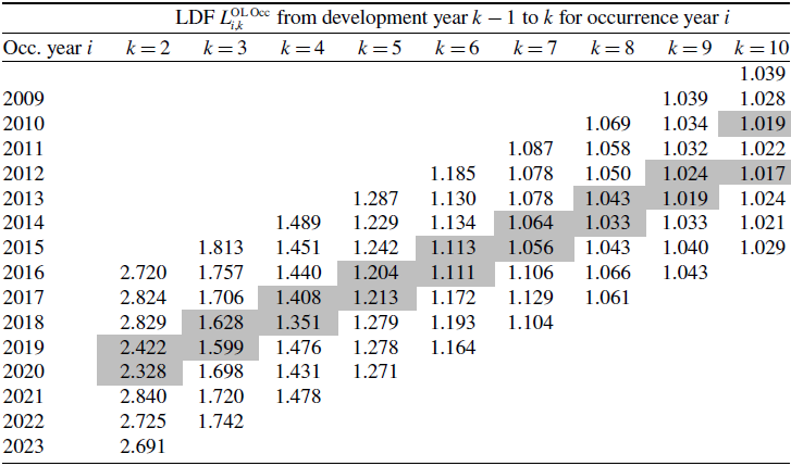
 Li,kOLOcc