INTRODUCTION
Canada emits about 0·02 of the global greenhouse gases (GHGs) (Neitzert et al. Reference Neitzert, Chiang Cheng, Collas, Matin, Folliet and Mckibbon2007). Of these emissions, agricultural methane (CH4) and nitrous oxide (N2O) account for approximately 0·08. Unlike in other sectors, GHGs from agriculture are primarily N2O and CH4, in roughly equal proportion when expressed in units of carbon dioxide equivalents (CO2e). Agriculture produces 0·25 and 0·66 of Canada's CH4 and N2O emissions, respectively (Neitzert et al. Reference Neitzert, Chiang Cheng, Collas, Matin, Folliet and Mckibbon2007). Approximately two thirds of Canada's agricultural emissions are from livestock (enteric fermentation, manure storage and handling and pasture, range and paddock manure), with the rest coming from fertilizers (both manure and synthetic fertilizers), plant residue decomposition and cropping practices (such as summerfallow and irrigation) (Collas & Liang Reference Collas and Liang2007). Since 1990, GHG emissions from enteric fermentation and manure management have increased by 39 and 23%, respectively, and N2O emissions from manure management and agricultural soils have increased by 32 and 10%, respectively (Collas & Liang Reference Collas and Liang2007). This observed increase in Canadian GHG emissions has been attributed to rising livestock populations and an increased use of synthetic nitrogen (N) fertilizer on farms (Collas & Liang Reference Collas and Liang2007). As agriculture is a significant contributor to the country's total GHG emissions, some of which are increasing, a reduction in the industry's GHG output would aid Canada in reaching its emission reduction targets.
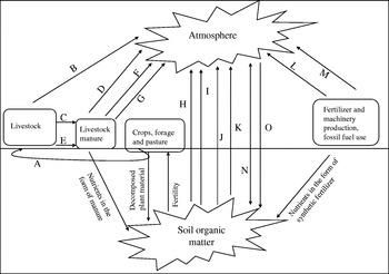
All sources of GHGs within the farming system need to be considered when assessing farm GHG emissions. Complex interactions exist between the processes, which produce each GHG (Fig. 1). Examining only one GHG ignores these interactions (Robertson & Grace Reference Robertson and Grace2004; Gregorich et al. Reference Gregorich, Rochette, VandenBygaart and Angers2005; Schils et al. Reference Schils, Verhagen, Aarts and Šebek2005), and the subsequent effect that changes in management practices may have on net farm GHG emissions. Moreover, farmers make decisions based on their entire farm – they have to look at how changes in one component may affect viability of other areas. As a result, whole-farm mitigation practices will be more readily accepted and adopted by producers than those that only focus on a small portion of the production system.
Diagram of the pools and flows contained within the model that was used in the present study. Flows are as follows: A=gross energy intake of cattle; B=enteric CH4 production by cattle; C=volatile solids excretion by cattle; D=CH4 production from manure; E=nitrogen excretion by cattle; F=direct N2O emissions from manure; G=indirect N2O emissions from manure; H=direct N2O emissions from land application of manure; I=indirect N2O emissions from land application of manure; J=direct N2O emissions from crop production; K=indirect N2O emissions from crop production; L=fossil fuel derived CO2 emissions from fuel usage and herbicide and machinery production; M=fossil fuel derived CO2 emissions from fertilizer production; N=soil carbon uptake/release; O=CH4 oxidation in agricultural soils.

The current paper focuses specifically on beef production systems because they are significant sources of GHGs, and hence, may represent important opportunities to reduce emissions. In 2005, Canadian beef cattle produced 21 Mt CO2e in enteric CH4 and 0·85 Mt CO2e CH4 from manure management (Collas & Liang Reference Collas and Liang2007). These systems are sources of three principal GHGs (CO2, CH4 and N2O), and can also be a sink for carbon (C). The objectives of the current paper were (i) to demonstrate the importance of looking at the whole-farm GHG emissions (rather than only from individual components); (ii) to compare the effects of changes in management practices on the net whole-farm GHG emissions and productivity from a beef production system; and (iii) to compare how net responses to selected practices vary among four different sites in western Canada. The underlying goal was to demonstrate the importance of a systems-based approach to reduce GHG emissions, rather than merely to provide estimates of emissions from various practices. For this purpose, a simple spreadsheet model was employed, although the findings may apply also to other systems-based modelling approaches.
MATERIALS AND METHODS
Four hypothetical farms, representing four diverse climatic and soil conditions on the Canadian prairies, were developed to provide the basis for evaluating GHG emissions. One farm was designed to represent each of the following locations, selected to provide a range of climatic conditions: (i) the southwestern region of Manitoba (MB farm), focusing on the area surrounding Deloraine, (ii) the Swift Current area in the south-central region of Saskatchewan (SK farm), (iii) the south-central area of Alberta, centred around Lethbridge (S.AB farm), and (iv) the Peace River region of northern Alberta (N.AB farm). Site-specific climate, yield, fertilizer and soil data were used to create the farms (Table 1). For each of these hypothetical farms, a baseline system (described below) was established, against which proposed changes, described in Table 2, were compared. Each farm, regardless of location, was designed to support the same number and type of cattle to allow comparisons among the farms. The baseline system for all farms included 100 hectares (ha) of barley, 230 ha of alfalfa-grass and 110 ha of pasture (0 ha fallow). The tillage system was assumed to be no-till, having changed from intensive tillage 15 years earlier. For livestock, the production year was split into three periods, with emissions from enteric fermentation and manure management calculated separately for each period. During Period 1 (136 days), from 16 October to 28 February, cattle were confined in corrals, the cows were pregnant but not lactating, calves from the previous spring were retained on-farm and fed forage-based diets (referred to as background calves), and replacement heifers were reared with the other calves. All animals were fed alfalfa-grass hay (11·9, 16·7 and 7·1 kg dry matter (DM)/head/day for cows, bulls and background calves, respectively). There were 100 cows, five bulls, 43 steers and 42 heifers on farm in Period 1. At the beginning of Period 1, 10 animals were culled from the herd and the previous year's replacement heifers joined the cow herd. The number of calves does not equal the number of cows, because of an assumed 15% calf loss annually. The background steers and heifers had an average daily gain (ADG) of 0·71 and 0·68 kg/head/day, respectively (Basarab et al. Reference Basarab, Okine, Baron, Marx, Ramsey, Ziegler and Lyle2005). During Period 2 (92 days), from 1 March until 31 May, cattle were kept in corrals; cows calved and began lactating, replacement heifers were moved into a separate group and, part way through Period 2, background calves were moved to the feedlot. Milk production was assumed to be 7·9 kg/day, milk fat was 47 g/kg and milk protein content was 35 g/kg (Butson & Berg Reference Butson and Berg1984). All cattle were fed alfalfa-grass hay (14·5, 16·7, 8·6 and 8·4 kg DM/head/day for cows, bulls, replacement heifers and background calves, respectively) except for feedlot cattle, which received barley (8·5 kg DM/head/day) and barley straw (2·0 kg DM/head/day). Replacement heifers had an ADG of 0·68 kg/day; background calves had the same ADG as in Period 1, until they reached the feedlot when ADG was increased to 1·59 kg/day for steers and 1·49 kg/day for heifers (Basarab et al. Reference Basarab, Okine, Baron, Marx, Ramsey, Ziegler and Lyle2005). During Period 2 there were 100 cows, 10 replacement heifers, 5 bulls, 75 background calves (early in the period) and 75 feedlot cattle (later in the period). During Period 3, from 1 June to 15 October, cows, replacement heifers and bulls were rotationally grazed on a grass pasture (14·0, 9·8 and 17·2 kg DM/head/day for cows, replacement heifers and bulls, respectively), while feedlot cattle remained confined and were fed barley (10·3 kg DM/head/day) and barley straw (2·0 kg DM/head/day). The cows were lactating, and cows and replacement heifers were bred. Milk production was assumed to be 5·8 kg/day, with milk fat and protein levels as before (Butson & Berg Reference Butson and Berg1984). Calves were weaned in early October. The ADG of cattle in the feedlot and replacement heifers was the same as that in Period 2 (Basarab et al. Reference Basarab, Okine, Baron, Marx, Ramsey, Ziegler and Lyle2005). In Period 3 there were 100 cows, 10 replacement heifers, 5 bulls and 75 feedlot cattle. During all periods the manure from cattle kept in corrals was stored in a deep bedding manure handling system (described in Intergovernmental Panel on Climate Change (IPCC) (Reference Eggleston, Buendia, Miwa, Ngara and Tanabe2006) ) and land applied in the fall.
Description of the hypothetical farms evaluated

* Landscapes of Canada Landscapes of Canada Working Group (2005).
† Marshall et al. (Reference Marshall, Schut and Ballard1999).
‡ Yield estimates were obtained from Manitoba Agriculture, Food and Rural Initiatives (2005) ; Saskatchewan Agriculture and Food (2007a, b); AAFRD (2007a, b, c). All yields were assumed to be dry weights. Yields of grass were the same as yields of alfalfa (Fairey Reference Fairey1991).
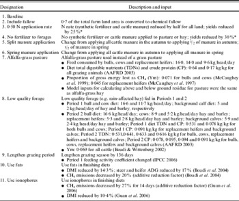
§ Rate=0·67×(max−min)+min of the range in AAFRD (2004).
Practices evaluated and some assumptions used in calculating emissions

* Estimated yield declines are somewhat arbitrary; actual yield losses with reduced fertilizer rates would vary widely.
Eleven management options were considered (Table 2): the baseline system (described in detail above) and 10 variations of the baseline. These 10 management strategies were selected as plausible alternatives to the baseline scenario. They were selected to illustrate the range and magnitude of potential responses, rather than as an exhaustive list of possible practices. Adjustments in practices such as fertilizer rates, therefore, were chosen to demonstrate how the system responds, rather than to advocate a recommended approach. The net emissions of each gas (t CO2e) as well as emissions per t of protein exported off-farm for each practice were compared with those of the baseline management scenario for each of the farms.
Cattle feed requirements and rations were based on Cowbytes software (Alberta Agriculture, Food and Rural Development (AAFRD) 2003). Crop and forage yields were then used to determine the area of each crop needed to meet the feed requirements of the cattle.
When management options affected yields, the land area needed to produce individual feedstuffs was adjusted. To maintain a consistent land base for comparison between scenarios and locations, farm size for the study was based on the location with the lowest yield and the scenario requiring the highest number of hectares to produce the feedstuffs needed to sustain the cattle.
The amount of manure produced by the livestock on-farm was also determined. Where the manure produced on-farm was insufficient to meet the target N requirements for crops (AAFRD 2004), supplementary synthetic fertilizer (both N and P) was applied.
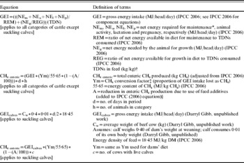
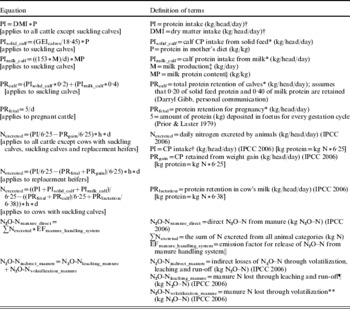
Enteric CH4 emissions were calculated for all categories of cattle on the farms. The CH4 production equation used was based on gross energy intake (GEI) of the cattle, which was calculated based on animal requirements and feed energy values (Table 3). Separate equations were used for calculating GEI and CH4 production for calves (Table 3). The proportion of GEI lost as CH4 (Ym) varied among categories of cattle; for example, a Ym value of 0·06 GEI (Boadi & Wittenberg Reference Boadi and Wittenberg2002) was used for cows and bulls kept in corrals, while a Ym value of 0·04 GEI (IPCC Reference Eggleston, Buendia, Miwa, Ngara and Tanabe2006) was used for cattle in the finishing phase. Although Ym values were changed to reflect changes in management, the value used for a given management strategy was consistent across all locations. Methane conversion values for the different animal types and scenarios were taken from IPCC (Reference Eggleston, Buendia, Miwa, Ngara and Tanabe2006) and from Canadian studies (McCaughey et al. Reference McCaughey, Wittenberg and Corrigan1997, Reference McCaughey, Wittenberg and Corrigan1999; Boadi & Wittenberg Reference Boadi and Wittenberg2002; Ominski et al. Reference Ominski, Boadi and Wittenberg2006). Coefficients for the effect of ionophores and fats on CH4 production, dry matter intake (DMI) and ADG were based on Boadi et al. (Reference Boadi, Wittenberg, Scott, Burton, Buckley, Small and Ominski2004) and Guan et al. (Reference Guan, Wittenberg, Ominski and Krause2006).
Equations used to calculate enteric CH4 emissions from beef cattle

* Average weight (kg): cows=591; bulls=1000; background steers and heifers: 276, 274 in Period 1, 344, 342 in Period 2; replacement heifers: 352 in Period 2, 430 in Period 3; feedlot steers and heifers: 393, 385 in Period 2, 518, 487 in Period 3; mature cow and bull weight=same as average weight; finished steer and heifer weight (kg)=615 and 568.
† Baseline TDN of: 0·61 kg/kg for confined cows, bulls, replacement heifers and background calves; 0·75 kg/kg for feedlot cattle; 0·641 kg/kg for grazing cows, bulls and replacement heifers (AAFRD 2003).
‡ Baseline Ym of: 0·06 for confined cows, bulls, replacement heifers and background calves (Boadi & Wittenberg Reference Boadi and Wittenberg2002); Ym of 0·04 for feedlot cattle (IPCC Reference Eggleston, Buendia, Miwa, Ngara and Tanabe2006); Ym of 0·095 for grazing cows and bulls (McCaughey et al. Reference McCaughey, Wittenberg and Corrigan1999); Ym of 0·87 for grazing replacement heifers (Ominski et al. Reference Ominski, Boadi and Wittenberg2006).
§ Baseline additive reduction factor=0.
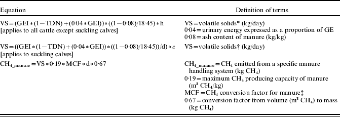
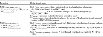
Calculations for CH4 emissions from cattle manure were based on the amount of volatile solids (VS) excreted, the length of storage (if any), the maximum CH4 producing capacity (Bo) of manure and a methane conversion factor (MCF) specific for the storage type used. The amount of VS excreted depended largely on GEI and on feed characteristics (Table 4); VS excretion from calves was calculated separately. Straw used as bedding is not included in the total VS or in the estimate of manure CH4 emissions (IPCC Reference Eggleston, Buendia, Miwa, Ngara and Tanabe2006). Since the use of straw is associated with solid manure storage systems, the contribution of the VS in straw to total CH4 emissions is minimal.
Equations used to calculate CH4 emissions from cattle manure in storage and deposited directly onto pasture by grazing animals (IPCC Reference Eggleston, Buendia, Miwa, Ngara and Tanabe2006)
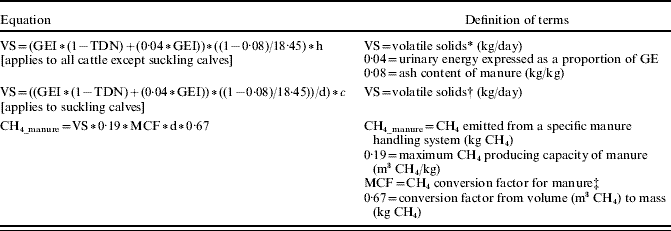
* Uses GEI from Table 3 that applies to all cattle except suckling calves.
† Uses GEI from Table 3 that applies to suckling calves.
‡ MCF=0·17 for deep bedding; 0·01 for pasture (IPCC Reference Eggleston, Buendia, Miwa, Ngara and Tanabe2006).
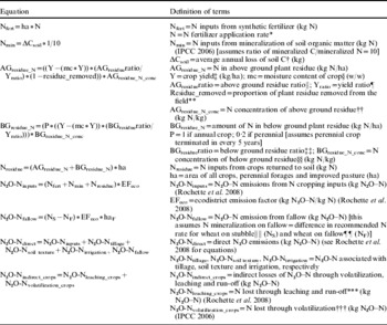
Nitrous oxide emissions from manure are affected by the amount of N excreted in the faeces and urine of cattle, which is a function of protein intake and protein retention by cattle (Table 5). Emissions are also affected by the length of the grazing season, which affects the amount of manure deposited directly onto pasture. Indirect N2O emissions, which emanate from N lost via leaching or volatilization, are related to the type of manure storage (manure kept in a drylot v. manure deposited on pasture by grazing animals). Leaching losses of zero were assumed for solid manure storage (Table 5). As there are no volatilization or leaching losses of straw N during solid manure storage (IPCC Reference Eggleston, Buendia, Miwa, Ngara and Tanabe2006), straw was not included in the estimates of manure storage N2O emissions.
Equations used to calculate direct and indirect N2O emissions from cattle manure in storage and on grazed pastures

* Equation obtained from Darryl Gibb (personal communication, Agriculture and Agri-Food Canada, Lethbridge, AB).
† Baseline crude protein content of: 0·14 kg/kg for confined cows, replacement heifers, bulls and background calves; 0·11 and 0·112 kg/kg for feedlot cattle in Periods 2 and 3, respectively; 0·125 kg/kg for grazing cows, bulls and replacement heifers (AAFRD 2003); see Materials and methods section for baseline DMI, Table 2 for any changes to DMI that occurred; PRgain for bulls is 0.
‡ Milk production (kg/head/day): Period 1=0; Period 2=7·9; Period 3=5·8 (Butson & Berg Reference Butson and Berg1984).
§ Milk protein=0·035 kg/kg (Butson & Berg Reference Butson and Berg1984).
‖ EFmanure_handling_system=0·01 for deep bedding and 0·02 for pasture (kg N2O–N/kg N) (IPCC Reference Eggleston, Buendia, Miwa, Ngara and Tanabe2006).
¶ Proportion of manure N lost during leaching: deep bedding=0; pasture=calculated (Rochette et al. Reference Rochette, Worth, Lemke, Mcconkey, Pennock, Wagner-Riddle and Desjardins2008); emission factor for N2O–N emissions from leaching=0·0125 kg N2O–N/kg N leached (IPCC Reference Penman, Kruger, Galbally, Hiraishi, Nyenzi, Emmanul, Buendia, Hoppaus, Martensen, Meijer, Miwa and Tanabe2001).
** Proportion of manure N lost during volatilization: deep bedding=0·30; pasture=0·20; emission factor for N2O–N emissions from volatilization=0·01 kg N2O–N/kg NH3–N+NOx–N volatilized (IPCC Reference Eggleston, Buendia, Miwa, Ngara and Tanabe2006).
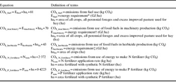
The N2O emissions (both direct and indirect) from land application of cattle manure were affected by the amount of N lost as N2O–N during manure storage, and the season of land application (Table 6). As straw used for bedding represents a source of additional N applied to land, N2O emissions from straw should be included with emissions resulting from land application of manure (IPCC Reference Eggleston, Buendia, Miwa, Ngara and Tanabe2006). For simplicity, N2O emissions from straw were estimated by making the assumption that no residue was removed from fields.
Equations used to calculate direct and indirect N2O emissions from land application of cattle manure

* EFfertilizer=0·007 in MB or N.AB; 0·001 in SK; 0·0167 in S.AB (derived from a compilation of published and unpublished measurement-based Canadian data (Philippe Rochette, Agriculture and Agri-Food Canada – Ste. Foy & Reynold Lemke, Agriculture and Agri-Food Canada – Swift Current)).
† If spring manure application, TFmanure_applied=1·0 in MB, SK or N.AB; 1·3 in S.AB; if fall manure application, TFmanure_applied=1·1 in MB, SK or N.AB; 1·8 in S.AB.
‡ Proportion of manure N lost during leaching: SK=0·05; MB, N.AB=0·10; S.AB=0·25 (IPCC Reference Eggleston, Buendia, Miwa, Ngara and Tanabe2006); emission factor for N2O–N emissions from leaching=0·0125 kg N2O–N/kg N leached (IPCC Reference Penman, Kruger, Galbally, Hiraishi, Nyenzi, Emmanul, Buendia, Hoppaus, Martensen, Meijer, Miwa and Tanabe2001).
§ Proportion of manure N lost during volatilization: 0·20 (IPCC Reference Eggleston, Buendia, Miwa, Ngara and Tanabe2006); emission factor for N2O–N emissions from volatilization=0·01 kg N2O–N/kg NH3–N+NOx–N volatilized (IPCC Reference Eggleston, Buendia, Miwa, Ngara and Tanabe2006).
Current estimates of N2O emission included N2O released from N inputs to the land (synthetic fertilizer, plant residue from the previous year and mineralization of native soil organic matter) and considered influences of tillage, fallowing, soil texture, climate and irrigation (Table 7). Indirect emissions from leaching, run-off and volatilization were also estimated. Estimated N2O emissions from N inputs were calculated for each crop type, whereas other sources of N2O emissions were calculated for the entire farm.
Equations used to calculate direct and indirect N2O emissions from crop production (grain crops, forages and pasture)

* See Table 1 for N fertilizer application rate. Synthetic fertilizer is only used on those hectares that did not receive cattle manure (calculated from animal feed characteristics).
† The sum of CO2-Ctillage+CO2-Cfrequency+CO2-Ccover+CO2-Cforage (Table 9).
‡ See Table 1 for crop yields for each crop on each farm.
§ Moisture content of: barley=0·12 kg/kg; alfalfa and alfalfa-grass=0·13 kg/kg; grass=0·13 kg/kg (Janzen et al. Reference Janzen, Beauchemin, Bruinsma, Campbell, Desjardins, Ellert and Smith2003).
‖ Above ground residue ratio: barley=0·47; alfalfa and alfalfa-grass=0·10; grass=0·12 (Janzen et al. Reference Janzen, Beauchemin, Bruinsma, Campbell, Desjardins, Ellert and Smith2003).
¶ Yield ratio: barley=0·38; alfalfa and alfalfa-grass=0·40; grass=0·18 (Janzen et al. Reference Janzen, Beauchemin, Bruinsma, Campbell, Desjardins, Ellert and Smith2003).
** 0 residue is removed from the field for both barley and alfalfa-grass hay. In fact, straw is removed from the barley field, but to include emissions from straw used for bedding, 0 residue removed was input.
†† Above ground residue N concentration: barley=0·007; alfalfa and alfalfa-grass=0·015; grass=0·016 (Janzen et al. Reference Janzen, Beauchemin, Bruinsma, Campbell, Desjardins, Ellert and Smith2003).
‡‡ Below ground residue ratio: barley=0·15; alfalfa and alfalfa-grass=0·50; grass=0·70 (Janzen et al. Reference Janzen, Beauchemin, Bruinsma, Campbell, Desjardins, Ellert and Smith2003).
§§ Below ground residue N concentration: barley=0·010; alfalfa and alfalfa-grass=0·015; grass=0·010 (Janzen et al. Reference Janzen, Beauchemin, Bruinsma, Campbell, Desjardins, Ellert and Smith2003).
‖‖ N fertilizer application rate for spring wheat (kg/ha) – stubble: MB=71; SK=54; S.AB=95; N.AB=71 (rate is 2/3 of the range for the crop and soil type given in AAFRD (2004) – calculation shown in Table 1).
¶¶ N fertilizer application rate for spring wheat (kg/ha) – fallow: MB=28; SK=17; S.AB=17; N.AB=28 (rate is 2/3 of the range for the crop and soil type given in AAFRD (2004) – calculation shown in Table 1).
*** Proportion of N lost via leaching was calculated using equations from Rochette et al. (Reference Rochette, Worth, Lemke, Mcconkey, Pennock, Wagner-Riddle and Desjardins2008) ; the emission factor for leached N was 0·0125 (IPCC Reference Penman, Kruger, Galbally, Hiraishi, Nyenzi, Emmanul, Buendia, Hoppaus, Martensen, Meijer, Miwa and Tanabe2001).
††† Proportion of N lost via volatilization was 0·1 and the emission factor was 0·01 (IPCC Reference Eggleston, Buendia, Miwa, Ngara and Tanabe2006).
CO2 emissions from fossil fuels used on-farm and for the production of machinery, herbicides and N and phosphorus (P) fertilizers (Table 8) were included. CO2 emissions from direct fuel use and production of machinery were based on the area of crops, forages, pasture and fallow and the energy use per hectare, with a unique energy use value associated with each crop type or fallow. A similar equation was used to calculate the CO2 emissions from herbicide production, with the assumption that it did not include the area of forages or pasture.
Equation used to calculate the fossil fuel-derived CO2 emissions from machinery, herbicide and fertilizer

* Efuel for crops: MB and N.AB=1·43; SK=1·42; S.AB=0·97; Efuel for fallow: MB and N.AB=0·93; SK and S.AB=0·34.
† Emachinery for crops: MB, SK and N.AB=0·48; S.AB=1·27; Emachinery for fallow: MB and N.AB=0·28; SK and S.AB=0·04.
‡ Eherbicide for crops: MB, SK and N.AB=0·46; S.AB=0·24; Eherbicide for fallow: MB and N.AB=0·60; SK and S.AB=0·78.
Efuel, Emachinery and Eherbicide are assumed values, based, in part, on E. Smith (personal communication).
CO2 emissions or removal were calculated in response to recent (within 20 years) changes in land management, including changes in tillage (applied to land in annual crop production only) (Table 9). In the scenario where fallow is included in the crop rotation, it was assumed there is zero soil C gain from no-till because the use of fallow tends to encourage C loss, perhaps offsetting some of the benefits of no-till (Janzen et al. Reference Janzen, Campbell, Izaurralde, Ellert, Juma, McGill and Zentner1998). Rates of soil C gain or loss vary widely, and approximate values are shown here primarily for illustrative purposes. In all scenarios, it was assumed no changes in frequency of perennial forage in rotations or conversion of cropped land to permanent cover in the last 20 years, so these practices had no effect on soil C. CO2 emissions resulting from straw addition to or removal from the land were not included in the current analysis. Uptake of CH4 by soils was assumed to be constant, at a rate of 0·325 kg CH4-C/ha/year for all land. Although this value has some uncertainty, its contribution to net whole-farm emissions is almost negligible (Ellert & Janzen Reference Ellert and Janzen2008).
Equations used to calculate the CO2 emissions or removal resulting from soil carbon change (estimates of soil C coefficients are approximate, and are provided mostly for illustrative purposes)

* CO2-Ctillage is zero when fallow is incorporated into the crop rotation; it was assumed that including fallow, which tends to reduce soil C content (Janzen et al. Reference Janzen, Campbell, Izaurralde, Ellert, Juma, McGill and Zentner1998), negates any benefits of using no-till.
† SCtillage=−0·19 for SK and S.AB; −0·365 for MB and N.AB; applies only to land in annual crop production.
The net whole-farm emissions were expressed both as t CO2 equivalent (CO2e) per farm and as t CO2e per t of protein exported off-farm in crop and animal products. Expressing emissions per unit of protein provides a common basis for comparing emissions across different farming systems. A protein content of 0·125, 0·140 and 0·078 kg/kg, for barley, alfalfa-grass hay and low quality forage, respectively (AAFRD 2003) was used. Grass pasture and alfalfa-grass pasture were assumed to have protein contents of 0·125 and 0·171 kg/kg, respectively. The value for grass pasture was an average of early season grass pasture and native pasture (AAFRD 2003). The estimated protein contents of finished steers, finished heifers and cull cows were 0·160, 0·159 and 0·158 kg/kg, respectively (Berg & Butterfield Reference Berg and Butterfield1976). The dressing percentage of steers, heifers and cull cows was 59·2, 57·7 and 49·5%, respectively (AAFRD 2007d). Protein in the animal tissue of cull cows and finished steers and heifers, as well as protein in any grain, forages or pasture, which were not fed to cattle were included in the protein exported off-farm. The pasture was rotationally grazed, with some portions of the grazing system left ungrazed. The area of pasture at all locations was large enough to support the animals for the entire grazing season for the practice with the largest land requirement in the least productive region; in some cases, therefore, there was more pasture than was required by the cattle. Where excess grass was produced, it was assumed that it was cut and baled for hay. Emissions were measured using protein exported off-farm rather than protein produced on-farm per se, because exported protein represents the net farm production.
Methane and N2O were converted to CO2e using a global warming potential of 23 and 296 (mass/mass), respectively (Ramaswamy et al. Reference Ramaswamy, Boucher, Haigh, Hauglustaine, Haywood, Myhre, Nakajima, Shi, Solomon, Houghton, Ding, Griggs, Noguer, van der Linden, Dai, Maskell and Johnson2001). All calculations were performed using Microsoft Excel© software.
RESULTS
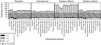
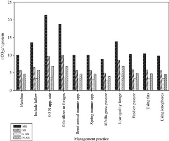
Net whole-farm emissions (t CO2e per farm) varied widely among farm locations (Fig. 2). The SK farm had the lowest emissions, with baseline net emissions of c. 706 t CO2e. The MB and N.AB farms had baseline net emissions of c. 758 and 761 t CO2e, respectively, and the S.AB farm had baseline net emissions of c. 1384 t CO2e. When expressed per unit of productivity, however, baseline emissions for MB, SK, S.AB and N.AB were 9·93, 5·65, 3·28 and 4·64 t CO2e per t of protein, respectively (Fig. 3).
GHG emissions (t CO2e) for each management practice on each of the four hypothetical farms.

GHG emissions per unit of protein exported off-farm (t CO2e/t protein) for each management practice on each of the four hypothetical farms.

The largest contributor to net emissions was CH4 on the MB, SK and N. AB farms and N2O on the S.AB farm (Fig. 2). The CH4 emissions were similar across all locations. The N2O emissions were similar for the MB and N.AB farms, with SK having slightly lower N2O emissions. The S.AB farm had N2O emissions that were several-fold greater than those of the MB, SK and N.AB farms, reflecting the higher soil moisture resulting from irrigation on the S.AB farm. The S.AB farm also had high CO2 emissions, due to more intensive energy use associated with irrigation.
Reducing fertilizer rates appreciably reduced overall emissions from farms. For example, the largest reductions in total emissions per farm (t CO2e) were achieved by eliminating fertilization of forages, at all locations (Fig. 2). Applying less N fertilizer (either by reducing the fertilizer application rate by half or eliminating fertilization of forages) significantly lowered N2O production and reduced overall emissions. This also lowered CO2 emissions from fuel use and machinery and synthetic fertilizer production, as fewer hectares of pasture were cut and baled for hay and less synthetic fertilizer was applied.
However, when productivity was taken into account (expressing GHG emissions per unit protein), reducing fertilizer rates often increased emissions. For example, reducing the fertilizer application rate by half resulted in the largest increase in emissions per t of protein on the MB farm, because of the decline in productivity. Similarly, eliminating fertilization of forages led to the largest rise in emissions per t of protein on the SK farm (Fig. 3). As a consequence of lower yields, more land is needed to meet the feed requirements of the cattle, leaving fewer hectares for other crops with saleable value. While reducing the amount of N fertilizer applied does reduce net emissions, it can increase emissions per unit protein because of suppressed yields (e.g. the MB and SK farms). The increase in emissions per unit protein resulting from decreased fertilizer rates that was observed on the MB and SK farms were less apparent on the S.AB and N.AB farms, presumably due to the higher yields at the latter locations.
Including 30 ha of fallow (and reducing the area of barley by the same amount) showed an increase in net farm emissions (t CO2e) on the MB, SK and N.AB farms (Fig. 2). Including fallow also increased emissions per unit protein (Fig. 3) because fallow reduced C sequestration (Grant et al. Reference Grant, Smith, Desjardins, Lemke and Li2004).
Pasturing cattle on an alfalfa-grass mix as opposed to grass only was the most effective practice for reducing emissions at each of the four locations when estimating emissions based on farm productivity (Fig. 3).
Feeding lower quality forage over the winter showed the greatest increase in net farm emissions (t CO2e) on the S.AB farm, and increased emission levels also at the other three farms (Fig. 2). This practice elicited the largest increase in emissions per unit protein (t CO2e/t protein) on the S.AB and N.AB farms (Fig. 3).
The timing of manure application had limited effect on emissions. For the SK farm, the model estimated no change in emissions for either splitting the land application of cattle manure between spring and autumn or land applying manure in the spring only, compared with the baseline management scenario (where all manure is land applied in the fall). For the other farms, land with half of the manure applied in the autumn and the other half in the spring and land with all of the manure applied in the spring decreased net farm emissions (Fig. 2) and emissions per unit protein (Fig. 3) when compared with the baseline scenario, but reductions were small.
Feeding cows and bulls on pasture from the middle of October until the end of February increased both net farm emissions (Fig. 2) and emissions per unit of protein (Fig. 3) at all farms, except S.AB where there was no change.
Adding fats to finishing diets slightly reduced overall net emissions (t CO2e) for all farms (Fig. 2) and increased emissions per unit protein by varying degrees at all locations (Fig. 3).
Including ionophores in the diet showed a slight decrease in emissions per unit protein when compared with the baseline at all locations. The model showed only a 0·76 t CO2e per t of protein decrease in CH4 production for all farms (Fig. 3).
DISCUSSION
The net atmospheric CO2 removal on the MB and N.AB farms was higher than that on the other farms because their soils (Black Chernozem and Gray Luvisol) tend to show higher rates of C accrual with improved practices (Boehm et al. Reference Boehm, Junkins, Desjardins, Kulshreshtha and Lindwall2004). (All estimates of soil C gain, however, are approximate, since they vary widely depending on a range of factors (Janzen et al. Reference Janzen, Campbell, Izaurralde, Ellert, Juma, McGill and Zentner1998).)
When fallow land was included as a management strategy, N2O emissions declined because of reduced fertilizer use, but the decreased N2O emissions were outweighed by increased CO2 emissions from soil C loss. As less land was in production, less protein was available for export from the farm, making emissions per unit protein higher. The resulting increase in GHG output demonstrates the importance of studying farming systems as a whole rather than only their component parts.
The reduction in t CO2e per t of protein observed when cattle were pastured on alfalfa-grass occurred primarily through reduced enteric CH4 emissions. The higher nutritive value of alfalfa, compared with grass, increases the rate of digestion. The increased dietary protein content and microbial N synthesis associated with alfalfa increases the amount of non-ammonia N that reaches the small intestine. This, along with the improved energy utilization associated with legume diets, improves overall digestive efficiency (Frame & Laidlaw Reference Frame, Laidlaw, Reynolds and Frame2005).
Feeding low quality forage increases CH4 production because it slows the rates of passage and ruminal fermentation, creating a high acetate:propionate ratio, which is conducive to CH4 production (Boadi et al. Reference Boadi, Wittenberg, Scott, Burton, Buckley, Small and Ominski2004). Slower passage rates reduce DMI, resulting in less fermentable substrate in the rumen, and therefore increase CH4 production (Johnson & Johnson Reference Johnson and Johnson1995; McAllister et al. Reference Mcallister, Okine, Mathison and Cheng1996). These processes, which increase CH4 production, were accounted for in the model by using a higher Ym value in this scenario than in the baseline scenario. Conversely, the N2O emissions were decreased due to the lower protein content of the feed and, consequently, the lower amounts of N present in the manure during storage and land application. However, the decrease in N2O emissions was not enough to counteract the large increase in enteric CH4 emissions.
Decreased emissions resulting when half or all of the cattle manure was land applied in spring, as opposed to full manure application in autumn, may be attributed to lower amounts of manure-N being present on the land during spring thaw, when most of the annual N2O emissions occur (Nyborg et al. Reference Nyborg, Laidlaw, Solberg and Malhi1997).
Enteric CH4 emissions increased when the grazing season was lengthened because cattle that are fed hay while on autumn/winter pasture have higher GEI's than confined cattle, but the lower MCF for manure deposited on pasture (v. stored) resulted in a net decrease in CH4 emissions. The MCF for stored manure is higher than for manure deposited directly on pasture because the anaerobic conditions and accumulation of organic matter that occur in manure storage are conducive to CH4 production (IPCC Reference Eggleston, Buendia, Miwa, Ngara and Tanabe2006). Manure N2O emissions increased because the N2O emission factor for manure deposited directly on pasture is greater than that for manure kept in storage, because of greater aeration in pasture-deposited manure (Jun et al. Reference Jun, Gibbs, Gaffney, Ngara, Miwa, Buendia, Tanabe and Pipatti2002). A shorter confinement period reduced the amount of cattle manure available for land application, resulting in the use of more synthetic fertilizer, and increased N2O and CO2 emissions. The overall effect of this practice, therefore, reflected the net effect of reduced CH4 emissions and enhanced N2O and CO2 emissions.
Fats in the diet reduce enteric CH4 production because they provide an alternative hydrogen sink to CO2 (Czerkawski et al. Reference Czerkawski, Blaxter and Wainman1966), inhibit certain ruminal microbial populations (National Research Council (NRC) 2001) and reduce fibre digestibility (McGinn et al. Reference McGinn, Beauchemin, Coates and Colombatto2004). Fatty acids serve as an alternative hydrogen sink to CO2, preventing the hydrogen from attaching to the CO2 to form CH4 (Czerkawski et al. Reference Czerkawski, Blaxter and Wainman1966). Some fat will remain unsaturated (NRC 2001), accumulate in the rumen and impede the ability of microflora to break down fibre (NRC 2001), reducing the fibre digestibility of forages and decreasing the amount of CH4 produced (McGinn et al. Reference McGinn, Beauchemin, Coates and Colombatto2004). Including fats in diets, however, can reduce ADG (Boadi et al. Reference Boadi, Wittenberg, Scott, Burton, Buckley, Small and Ominski2004) and, by extending the length of time animals were in the feedlot, this resulted in more feed consumed and less feed available for sale off-farm. Keeping the animals in the feedlot longer also increased the CH4 and N2O emissions from manure because more manure was produced.
Including fats in finishing diets does not always lead to a reduction in DMI and ADG (Mir et al. Reference Mir, Mir, Kuber, Gaskins, Martin, Dodson, Elias Calles, Johnson, Busboom, Wood, Pittenger and Reeves2002), but the present results are based on Boadi et al. (Reference Boadi, Wittenberg, Scott, Burton, Buckley, Small and Ominski2004), which may be the study most relevant to the current setting. Clearly, this potential mitigation practice merits more research attention, particularly because of apparent responses in both CH4 and productivity, and the apparent sensitivity of that response to rate of amendment.
Rumen micro-organisms can adapt to ionophores and, after a short period, the rumen bacteria start producing CH4 again (Chen & Wolin Reference Chen and Wolin1979). Most of the observed decrease in overall emissions that occurred when including ionophores in finishing diets reflected reduced N2O emission from a decrease in manure N (less manure was produced as the animals have a lower DMI when consuming ionophores with a high concentrate diet (Guan et al. Reference Guan, Wittenberg, Ominski and Krause2006)). Ionophores are not a long-term solution for reducing enteric CH4 emissions because of methanogens' ability to adapt to them, and the increasing public pressure to reduce the use of antimicrobials in animal production (Beauchemin et al. Reference Beauchemin, Kreuzer, O'mara and McAllister2008).
The current study shows the importance of looking at the beef production system as a whole, considering all gases, and all facets of the farm. For example, use of low quality forages on the MB farm increased CH4 emissions by approximately 56 t CO2e but reduced N2O emissions by almost 25 t CO2e. Focusing on only one of the gases might distort the benefits of the practice. In another example, feeding cows and bulls on pasture from the middle of October until the end of February increases enteric CH4 emissions, but these are more than offset by a decrease in manure CH4; in this instance, evaluating only enteric CH4 emissions might yield the wrong recommendation, as there was a net decrease in CH4 emissions. Similar examples where emissions from one source increased while others decreased are the scenarios where (i) fallow was included and (ii) where the pasture was alfalfa-grass rather than grass. All of these examples stress the importance of considering whole-farm emissions when examining the benefit of a proposed mitigation practice.
Because of the responsiveness of GHG emissions to local conditions and practices, the location of the farm plays an important role in determining the relative importance of the various GHGs. For example, the analysis demonstrates that CH4 contributes a large proportion of the net farm CO2e on the MB, SK and N.AB farms and, therefore, management practices focusing on reducing emissions of CH4 would lead to the largest reductions in GHG output. However, for the S.AB farm, N2O is the largest GHG contributor and practices aimed at reducing N2O emissions might be most urgent there.
The effectiveness of practices in reducing predicted GHG emissions varied, depending on location. For example, changing the timing of manure application had less effect on the SK farm than on the MB, S.AB and N.AB farms. Also, eliminating fertilization of forages showed small increases in emissions per unit protein on the S.AB and N.AB farms but relatively large increases in emissions on the MB and SK farms. These observations suggest that there can be no universally applicable set of best management practices – the practices that best reduce emissions depend on the location of the farm.
The variability of the effectiveness of practices among sites suggests the possibility of using resources more efficiently by focusing on those sites that are most responsive. For example, the current analysis, if acceptable, suggests that mitigation efforts on farms like MB might merit more attention than similar practices on farms like S.AB.
The current analysis suggests, further, that the net overall effect of mitigative practices, at least those evaluated, was often small. For example, the practices evaluated at the SK site reduced net emissions by 11%, at best, relative to the baseline scenario. In part, this observation may reflect the multiple processes of GHG formation in farming systems. By virtue of the numerous processes, and the complexity of their interactions, it may be possible to reduce emissions from one source appreciably, but that benefit may be partly offset or at least dwarfed by emissions from another source.
Expressing emissions in terms of t CO2e per t of protein changed the ranking of the different locations (baseline scenario). The MB farm, which had the second lowest net farm emissions (t CO2e), was the highest emitter when farm productivity was accounted for, and the S.AB farm, which had the highest net farm emissions, was the lowest GHG producer when productivity was considered because of the higher crop yields.
Reporting emissions in terms of farm productivity may be more pertinent because it describes the environmental cost of that product more accurately. Choosing mitigation practices based simply on total net emissions might be misleading, because this could favour practices that reduce productivity. For example, in the scenario where the N application rate was cut in half for all crops, the net emissions (t CO2e) decreased at all four farms, but emissions per t of protein increased as a result of lost productivity. Similar results were observed for the scenario where zero fertilizer was applied to forages and pasture. Comparing management practices based on emissions per unit of protein identifies those practices and conditions with highest efficiency – those that yield highest productivity per unit of GHG emission. Furthermore, expressing emissions per unit protein may minimize ‘leakage’ – the phenomenon whereby reduced emissions from lower productivity at one site are merely shifted to sites elsewhere that provide compensatory production.
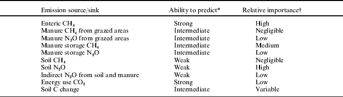
Farms are complex ecosystems and estimating net emissions requires numerous assumptions and empirical equations, many of which have significant uncertainty (Table 10 gives current estimates of the uncertainty in each area of the model used in the current study). The estimates in the current paper are still approximate and subject to further research, measurements and modification. With more research and scientific advances, many of the implicit assumptions and coefficients will no doubt change, likely modifying the predicted values. For example, rates of soil N2O emissions may be particularly tenuous and in need of further research (Table 10). These uncertainties, however, do not diminish the value of this analysis in illustrating the importance of trying to capture whole-farm influences when evaluating proposed mitigation practices. Moreover, such whole-farm analyses help to identify those facets of farms that merit the most urgent scientific scrutiny.
The status of the general ability to predict GHG emissions from beef production systems, and the relative importance of each component
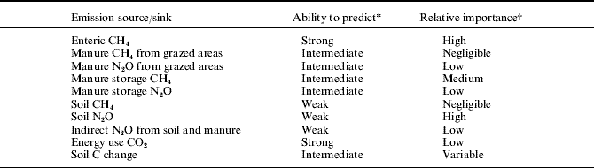
* Indicators are rough qualitative estimates of our ability to measure or predict GHG emissions. Indicator values of uncertainty are: strong, <0·10 (expressed as a proportion of the value); intermediate, 0·10–0·40; weak, >0·40.
† Estimated values of: high, >0·35; medium, 0·21–0·35; low: 0·05–0·20; negligible, <0·05 of total emissions on typical beef production farms, similar to those described in the present paper.
CONCLUSION
The model used in the present study will benefit from enhanced understanding that will come with further research. At present, it demonstrates, despite its uncertainties, that a whole-system approach is essential for evaluating the practices that best reduce emissions. Although current predicted estimates are not necessarily conclusive, they do illustrate that the ‘best’ practice depends on where the farm is located; there may be no universally applicable set of best management practices. Finally, the current exercise illustrates that expressing emissions per unit of protein might prevent the recommendation and subsequent utilization of mitigation practices that reduce emissions at the expense of restricted productivity.