





1 Introduction
Lyapunov exponents describe the exponential growth or decay of norms of products of matrices which in many settings are used to determine different ergodic and dynamical properties of the system. The question of existence of a non-zero exponent has been widely studied with such applications in mind. A further question is whether all Lyapunov exponents have multiplicity
$1$
 , referred to as simple Lyapunov spectrum, which provides more detailed information on ergodic averages, and implies in many settings the existence of one-dimensional invariant foliations for the system.
The study of criteria for non-zero exponents and simple spectrum for independent and identically distributed (i.i.d.) random products of matrices traces back to works of Furstenberg [Reference FurstenbergFur63], Guivarc’h and Raugi [Reference Guivarc’h and RaugiGR86], Gol’dsheid and Margulis [Reference Gol’dsheid and MargulisGM89], and Ledrappier [Reference LedrappierLed86], among many others. In all of these works, a common feature is an irreducibility hypothesis on the set of matrices generating the random products which ensures that cancelations of the expanding and contracting directions of the matrices do not occur almost surely. Under such irreducibility hypotheses, their theorems give existence of a non-zero Lyapunov exponent [Reference FurstenbergFur63] or simple spectrum [Reference Guivarc’h and RaugiGR86], provided that the matrices generating the products satisfy necessary contraction and expansion properties. For an overview of the Lyapunov exponents of i.i.d. matrix products, see [Reference Bougerol and LacroixBL85, Reference Benoist and QuintBQ16].
Motivated by applications for partially hyperbolic systems and holomorphic foliations, these criteria were later extended [Reference Bonatti, Gómez-Mont and VianaBGMV03, Reference Bonatti and VianaBV04] and refined [Reference Avila and VianaAV07a, Reference Avila and VianaAV07b] to apply to the setting of fiber-bunched matrix cocycles, where the product of matrices is formed as a skew product over a driving hyperbolic dynamical system, giving non-trivial and simple Lyapunov spectrum with respect to any measure satisfying a natural assumption known as local product structure. Fiber-bunching is a partial hyperbolicity-type condition which ensures the existence of holonomies for the cocycle, which in turn allows for many of the random features from the i.i.d. setting to apply in this setting.
In these works, the criteria found for non-trivial (that is, not all zero) or simple (that is, all distinct) Lyapunov exponents is a concrete setup, expressed as a transversality condition, which provides sufficient criterion for the existence of non-zero exponents [Reference Bonatti, Gómez-Mont and VianaBGMV03] and simple spectrum [Reference Bonatti and VianaBV04], respectively. These criteria in turn have been used to prove simplicity of spectrum generically for fiber-bunched cocycles over hyperbolic systems [Reference Avila and VianaAV07a], for certain cocycles over partially hyperbolic systems [Reference Poletti and VianaPV19], and for fiber-bunched Anosov flows and geodesic flows in pinched negative curvature [Reference MitsutaniMit22]. It has also been applied to specific situations such as in the solution of the Kontsevich–Zorich conjecture in Teichmüller dynamics [Reference Avila and VianaAV07b].
All criteria found so far for simple spectrum with respect to all reasonable measures in the fiber-bunched setting have only been sufficient criteria, in the form of existence of a particular setup over a periodic point. The goal of this paper is to provide a criterion for fiber-bunched cocycles over hyperbolic systems to satisfy simple Lyapunov spectrum with respect to a natural class of measures under an irreducibility hypothesis in the spirit of Guivarc’h and Raugi [Reference Guivarc’h and RaugiGR86]. The advantage of this approach is that an irreducibility hypothesis is evidently a necessary condition to guarantee that all measures have simple Lyapunov spectrum for a non-trivial reason.
Our main result shows that an irreducible fiber-bunched cocycle with one reasonable measure with simple Lyapunov spectrum in fact must have simple Lyapunov spectrum with respect to all reasonable measures.
Theorem A. Let
$\hat {\Sigma }$
 be a transitive invertible subshift of finite type and
$\hat {A}\colon \hat {\Sigma }\to \mathrm {SL}(d,\mathbb R)$
 be a fully irreducible Hölder continuous fiber-bunched cocycle. Suppose there exists an ergodic, fully supported, invariant measure
$\hat {\mu }$
 with continuous local product structure on
$\hat {\Sigma }$
 with simple Lyapunov spectrum. Then any other ergodic, fully supported, invariant measure
$\hat \eta $
 with continuous local product structure on
$\hat {\Sigma }$
 also has simple Lyapunov spectrum.
The complete definitions in the theorem above are provided in §2. The precise definition of full irreducibility is given in §3. We will actually prove a finer result than Theorem A. Namely, Theorem A is proved by individually showing that each Lyapunov exponent must have multiplicity 1 in the theorem below. We write
$\mathrm {Gr}(k,d)$
 for the Grassmannian of k-dimensional subspaces in
$\mathbb R^d$
 .
Theorem B. Let
$1 \leq k \leq d-1$
 ,
$\hat {\Sigma }$
 a transitive subshift of finite type and
$\hat {A}\colon \hat {\Sigma }\to \mathrm {SL}(d,\mathbb R)$
 a Hölder continuous fiber-bunched cocycle strongly irreducible on
$\mathrm {Gr}(k,d)$
 and on
$\mathrm {Gr}(d-k, d)$
 .
Suppose there exists an ergodic, fully supported, invariant measure
$\hat {\mu }$
 on
$\hat {\Sigma }$
 with continuous local product structure and
$\unicode{x3bb} _k(\hat {\mu })> \unicode{x3bb} _{k+1}(\hat {\mu })$
 . Then any other ergodic, fully supported, invariant measure
$\hat \eta $
 with continuous local product structure on
$\hat {\Sigma }$
 also has
$\unicode{x3bb} _k(\hat \eta )> \unicode{x3bb} _{k+1}(\hat \eta )$
 .
Full irreducibility is defined as strong irreducibility on
$\mathrm {Gr}(k,d)$
 for each
$1 \leq k \leq d-1$
 , so it is clear that Theorem A follows from Theorem B. The precise definition of strong irreducibility on
$\mathrm {Gr}(k,d)$
 is also given in §3, but we include a quick discussion on irreducibility conditions below.
Strong irreducibility was first defined in [Reference FurstenbergFur63] to study the existence of a positive Lyapunov exponent for an i.i.d. product of matrices as the condition that no union of proper subspaces of
$\mathbb R^d$
 is preserved by all matrices in the support of the distribution. As indicated before, this condition ensures that cancelations of expansion and contraction do not occur in smaller invariant subspaces. Generalizing Furstenberg’s theorem to study simplicity of the Lyapunov spectrum in the i.i.d. setting, in [Reference Guivarc’h and RaugiGR86] the authors consider the same condition but on exterior powers
$\Lambda ^k (\mathbb R^d)$
 . Later, in [Reference Avila and VianaAV07a, Reference VianaVia14], it was shown that this condition can be defined on Grassmannians using the embedding of
$\mathrm {Gr}(k,d)$
 in
$\Lambda ^k (\mathbb R^d)$
 . In the i.i.d. setting, strong irreducibility on
$\mathrm {Gr}(k,d)$
 is a less stringent requirement than strong irreducibility on
$\Lambda ^k (\mathbb R^d)$
 . Moreover, working on Grassmannians provides a clearer geometric interpretation of invariant objects as Lyapunov subspaces, and further, in [Reference VianaVia14] it is shown that strong irreducibility on
$\mathrm {Gr}(k,d)$
 is equivalent to a transversality condition known as twisting.
For these reasons, we work with strong irreducibility on Grassmannians. Our main strong irreducibility definition (Definition 3.2) is precisely this strong irreducibility on Grassmannians, but for a continuous linear cocycle we require non-existence of a continuous cocycle-invariant section of appropriate subspaces of
$\mathrm {Gr}(k,d)$
 , as opposed to the non-existence of appropriate subspaces of
$\mathrm {Gr}(k,d)$
 invariant by all matrices in the support of the distribution required in the i.i.d. case.
Remark 1.1. Although requiring a condition on
$\mathrm {Gr}(k,d)$
 and
$\mathrm {Gr}(d-k,d)$
 in Theorem B might seem unexpected, one may compare with [Reference Bonatti and VianaBV04, Theorem 1], which under a certain twisting condition establishes simultaneously that both the top and bottom Lyapunov exponent are one-dimensional.
In [Reference Bonatti, Gómez-Mont and VianaBGMV03, Theorem 1], Bonatti, Gomez-Mont, and Viana prove an alternative for fiber-bunched cocycles: either every equilibrium state has at least two distinct Lyapunov exponents or there exists a holonomy-invariant, cocycle-invariant measure on its projective extension. This, in turn, should imply either a failure of irreducibility or conformality of the cocycle (which implies that all exponents are
$0$
 for all invariant measures). For the sake of completeness, we include this statement in the following theorem.
Theorem C. Suppose that
$\hat {\Sigma }$
 is a transitive hyperbolic system and that
$\hat {A}\colon \Sigma \to \mathrm {SL}(d,\mathbb R)$
 is a fiber-bunched Hölder continuous cocycle that is strongly irreducible (on
$\mathrm {Gr}(1,d)$
 ). Then exactly one of the following assertions holds:
-
(1) for every measure $\hat {\mu }$
 with full support and continuous product structure,
$\hat {\mu }$
has two distinct Lyapunov exponents; or
-
(2) $\hat {A}$
preserves a Hölder continuous conformal structure, and thus every invariant measure has all Lyapunov exponents equal to
$0$
.


In view of this theorem, Theorem B above is a version of this result which extends to the study of every Lyapunov exponent, and thus to the study of simplicity of Lyapunov spectrum.
1.1 Prior results
To better frame the results of this paper, we now discuss in some detail some of the earlier results mentioned above. We begin with a review of the case of i.i.d. matrix products. Throughout, we let
$(A_1,\ldots ,A_m)\subseteq \mathrm {SL}(d,\mathbb R)$
 ,
$d\ge 2$
 , and let G denote the semigroup generated by the matrices
$A_1,\ldots ,A_m$
 .
The foundational result on the existence of non-zero Lyapunov exponents is the theorem of Furstenberg [Reference FurstenbergFur63]: if G is not compact and G acts strongly irreducibly on
$\mathbb R^d$
 , that is, G does not preserve a non-trivial finite union of subspaces of
$\mathbb R^d$
 , then almost surely the independent and uniformly distributed random products of the matrices in
$A_1,\ldots ,A_m$
 have two distinct Lyapunov exponents. Guivarc’h and Raugi [Reference Guivarc’h and RaugiGR86] improve on this theorem to obtain a criterion for simplicity of the top Lyapunov exponent. They prove that if G acts strongly irreducibly on
$\mathbb R^d$
 and there exists a sequence of elements
$g_n\in G$
 such that
$\|g_n\|^{-1}g_n$
 converges to a rank
$1$
 matrix, then
$\unicode{x3bb} _1>\unicode{x3bb} _2$
 . This implies a related result for
$\unicode{x3bb} _k>\unicode{x3bb} _{k+1}$
 by considering the associated action on
$\Lambda ^k(\mathbb R^d)$
 . Finally, Gol’dsheid and Margulis [Reference Gol’dsheid and MargulisGM89] improve this theorem to only have a hypothesis on the algebraic closure X of G in
$\mathrm {SL}(d,\mathbb R)$
 . All of the theorems above can be seen as presenting an alternative under an irreducibility hypothesis.
In [Reference Avila and VianaAV07b], the Lyapunov exponents of a locally constant cocycle over a shift equipped with a measure having a type of product structure are considered. The authors show that this cocycle has simple Lyapunov spectrum if it is pinching and twisting. Here, pinching and twisting reduce to an irreducibility condition on k-planes as well as a condition that says one can separate the singular value of matrices in the sense that for all
$K>0$
 , one can find an element A the cocycle acts by such that
$\sigma _k(A)>K\sigma _{k+1}(A)$
 . In [Reference Cambrainha and MatheusCM16], it is shown that almost every locally constant symplectic cocycle has simple spectrum.
Outside of the locally constant setting, it is more difficult to obtain results about Lyapunov exponents of cocycles. We describe here work studying fiber-bunched cocycles over hyperbolic bases. In [Reference Bonatti, Gómez-Mont and VianaBGMV03], those authors show that there is an open and dense subset of the space of fiber-bunched cocycles such that for every equilibrium state there are two distinct Lyapunov exponents by identifying a particular obstruction to hyperbolicity: a family of f-invariant, holonomy-invariant probability measures on every fiber of the bundle
$\Sigma \times \mathbb {RP}^{d-1}$
 that the cocycle acts on. Note that the result of [Reference Bonatti, Gómez-Mont and VianaBGMV03] does not offer any information about which two Lyapunov exponents might be distinct nor their multiplicity. See also [Reference Avila, Santamaria and VianaASV13, Theorem B], where a similar result is obtained for cocycles over partially hyperbolic systems with
$0$
 center exponents. In [Reference VianaVia08], Viana shows, without a fiber-bunching assumption, that for a fixed ergodic measure with product structure almost all Hölder continuous cocycles have two distinct Lyapunov exponents.
In the fiber-bunched setting, a pinching and twisting condition is sufficient for a fiber-bunched cocycle to have simple spectrum. In [Reference Bonatti and VianaBV04], it is shown that a generic fiber-bunched cocycle over a hyperbolic system has simple Lyapunov spectrum. This paper is one of the first where a type of pinching and twisting for fiber-bunched cocycles appears. In [Reference Avila and VianaAV07a], a simpler formulation of the pinching and twisting condition is given. Pinching and twisting has seen great application in the study of simplicity of Lyapunov spectrum. In [Reference Backes, Poletti, Varandas and LimaBPVL20], it is shown that one can adapt the pinching and twisting criterion of Avila and Viana in order to show that, in a particular sense, generic cocycles over non-uniformly hyperbolic systems have simple Lyapunov spectrum. In [Reference Bessa, Bochi, Cambrainha, Matheus, Varandas and XuBBC
+
18], a version of [Reference VianaVia08] for cocycles taking value in a semi-simple Lie group is proved, which says that a generic cocycle has two distinct Lyapunov exponents even when the cocycle lies, for example, in
$\mathrm {Sp}(n,\mathbb R)$
 . In [Reference Poletti and VianaPV19], the twisting and pinching criterion is extended to apply to cocycles over certain partially hyperbolic diffeomorphisms.
1.2 Discussion
When studying an abstract hyperbolic system, there is not always an obvious choice of measure that is the correct one to equip the system with. However, from the point of view of the thermodynamic formalism, equilibrium states provide the most natural choice of a measure. Consequently, it is conceptually satisfying to find criteria that apply to all these measures simultaneously.
On a technical level, this paper develops an approach to studying the Lyapunov exponents of fiber-bunched cocycles that uses a different sort of ‘twisting’ condition. In [Reference Avila and VianaAV07b], the twisting condition requires that the cocycle holonomy around a particular homoclinic loop satisfies a specific condition that it can move subspaces off of themselves. This condition is localized to a very specific periodic point
$\hat p$
 . In our setup, we have a measure
$\hat {\mu }$
 that has simple spectrum and another measure
$\hat \eta $
 that we are interested in showing has simple spectrum. By using the Oseledec subspaces of
$\hat {\mu }$
 we are able to obtain a sort of non-uniform twisting condition that is not localized near any particular point of
$\hat {\Sigma }$
 . The Oseledec subspaces associated to
$\hat {\mu }$
 are, in a certain sense, randomly distributed along local stable and unstable sets (See §3.1). Our main technical contribution is figuring out how to use this feature in order to show convergence to a Dirac measure in §4.
In this paper, we take as a hypothesis that ‘pinching’ occurs for a fully supported measure with continuous product structure. It remains interesting to determine if one can obtain the same conclusions from the existence of just a single ‘pinching’ orbit.
1.3 Structure of paper
Section 2 contains all necessary definitions and some standard constructions. In §3 we state our irreducibility hypothesis for fiber-bunched cocycles and show that it implies the random distribution of unstable subspaces as well as a corresponding statement about u-states. Finally, §§4 and 5 contain the proof of Theorem B and §6 contains the proof of Theorem C.
2 Background and definitions
For
$m\ge 2$
 , we let
$M = (q_{ij})$
 be an irreducible
$m\times m$
 matrix with entries in
$\{0,1\}$
 . Let
$\hat {\Sigma }$
 be the two-sided subshift of finite type associated to M, and
$\hat {\sigma } \colon \hat {\Sigma }\to \hat {\Sigma }$
 be the left-shift map. One can formulate an abstract notion of a hyperbolic system that generalizes the dynamical properties of this system (see, for example, the setting described in [Reference KalininKal11]), but we work with shifts here. The space
$\hat {\Sigma }$
 is endowed with a metric given for
$\hat {x}\neq \hat y$
 by

We will use the usual notation for cylinder sets where
$[0;i]$
 denotes the cylinder with zeroth symbol i. We write
$\Sigma $
 for the one-sided left shift associated to
$\hat {\Sigma }$
 .
We define the local stable and unstable sets of a point
$\hat {x}\in \hat {\Sigma }$
 :

We let
$\pi _s$
 and
$\pi _u$
 be the obvious projections onto the local stable and unstable sets. The global stable and unstable sets are defined similarly for
$\hat {x}\in \hat {\Sigma }$
 :

For two points
$\hat {x},\hat y$
 in the same cylinder
$[0;i]$
 we can take their Smale bracket
$[\hat {x},\hat y]$
 which is the unique point in
$W^u_{\mathrm {loc}}(\hat {x})\cap W^s_{\mathrm {loc}}(\hat y)$
 . Symbolically this point is given by the sequence

We will also work with one-sided shift spaces
$\Sigma ^s$
 and
$\Sigma ^u$
 . These are defined by


with the corresponding left and right shifts
$\sigma _u$
 and
$\sigma _s$
 . We also have notation for cylinders in
$\hat {\Sigma }$
 :

Analogously we define
$[m;a_0,\ldots ,a_k]^u$
 and
$[m;a_0,\ldots ,a_k]^s$
 as notation for cylinders in
$\Sigma ^u$
 and
$\Sigma ^s$
 . Since many arguments are symmetric for the left and right shift, whenever we need to consider only one of them at a time, say the left shift, in keeping with the literature we will also write
$\Sigma ^u$
 as
$\Sigma $
 and write P for the projection
$P\colon \hat {\Sigma }\to \Sigma $
 . Thus, symbols with hats are used for two-sided objects and symbols without hats for the corresponding one-sided objects on the left shift
$\Sigma ^u$
 .
We let
$\hat {A}\colon \hat {\Sigma }\to \mathrm {GL}(d,\mathbb R)$
 be an
$\alpha $
 -Hölder continuous function. We think of
$\hat {A}$
 as defining a cocycle
$\hat {\mathcal { A }}\colon \hat {\Sigma }\times \mathbb R^d\to \hat {\Sigma }\times \mathbb R^d$
 in the usual way and make the standard abuse of calling
$\hat {A}$
 a cocycle. We define for
$n\in {\mathbb N}$
 ,

and for
$n\in {\mathbb N}$
 also define
$\hat {A}^{-n}(\hat {x})=(\hat {A}^n(\hat {\sigma }^{-n}\hat {x}))^{-1}$
 as is standard.
In this paper we study fiber-bunched cocycles.
Definition 2.1. We say that an
$\alpha $
 -Hölder cocycle
$\hat {A}\colon \hat {\Sigma }\to \mathrm {GL}(d,\mathbb R)$
 is fiber-bunched if for every
$\hat {x}\in \hat {\Sigma }$
 ,

Fiber-bunched cocycles have a number of nice properties. The most important of which is that the cocycle has holonomies. See, for example, [Reference SadovskayaSad15, §4.2].
Proposition 2.2. Suppose that
$\hat {A}$
 is a fiber-bunched cocycle over
$\hat {\sigma }$
 . Then for any
$\hat {x}\in W^s_{\mathrm {loc}}(\hat y)$
 ,

exists and
$H^s_{\hat {x}\hat y}$
 , called the stable holonomy, defines a Hölder continuous function from
$x,y$
 to
$\mathrm {GL}(d,\mathbb R)$
 . The local stable holonomy satisfies:
-
(1) $H^s_{\hat {x}\hat {x}}=\mathrm {id}$
and
$H^s_{\hat y\hat z}\circ H^s_{\hat {x}\hat z}=H^s_{\hat {x}\hat z}$
for any
$\hat y,\hat z\in W^s_{\mathrm {loc}}(\hat {x})$
; -
(2) $\hat {A}(\hat {x})=H^s_{\hat {\sigma }(\hat y) \hat {\sigma }(\hat {x})}\circ \hat {A}(\hat y)\circ H^s_{\hat {x}\hat y}$
.




The analogous statement holds for the local unstable sets and their holonomies.
We will also make use of a global stable holonomy. For a point
$\hat {x}\in W^s(\hat y)$
 this is defined as follows. Iterate the cocycle until
$\hat {\sigma }^n(\hat {x})\in W^s_{\mathrm {loc}}(\hat {\sigma }^n(\hat y))$
 , then using this n, set

where the holonomy on the right-hand side is given by Proposition 2.2.
Using holonomies, via a construction which we recall now from [Reference Avila and VianaAV07a], we may assume that the cocycle is constant along local stable sets, so that
$\hat {A}$
 induces a cocycle over
$\Sigma ^u = \Sigma $
 . Fix some arbitrary point
$x^- \in \Sigma ^s$
 , the left-sided shift, and for each
$\hat {x} \in \hat {\Sigma }$
 let
$\phi ^u(\hat {x})$
 be
$W^u_{\mathrm {loc}}(x^-) \cap W^s_{\mathrm {loc}}(\hat {x})$
 . Then
$A(\hat {x})$
 , the reduced cocycle, is defined by

and
$\hat {x} \to A(\hat {x})$
 is easily seen to be constant along local stable manifolds due to (2) in Proposition 2.2.
2.1 Lyapunov exponents
For
$\hat {\mu }$
 any shift-invariant measure on
$\hat {\Sigma }$
 and
$\hat {A}: \hat {\Sigma } \to \mathrm {GL}(d,\mathbb R)$
 any measurable cocycle such that
$\int _{\hat {\Sigma }} \log ^+ \|\hat {A}^{\pm 1}\|\, d\hat {\mu } < \infty $
 , where
$\log ^+(x)=\max (0,x)$
 , the Oseledec theorem guarantees the existence of numbers

and an
$\hat {A}$
 -invariant measurable splitting
$\mathbb R^d = E_{d_1}(\hat {x}) \oplus \cdots \oplus E_{d_k}(\hat {x})$
 defined
$\hat {\mu }$
 -almost everywhere (
$\dim E_{d_i} = d_i - d_{i-1}$
 for
$i = 2, \ldots , k$
 and
$\dim E_1 = d_1$
 ), where the numbers
$d_i$
 correspond to the indices such that
$\unicode{x3bb} _{d_i}(\hat {\mu })> \unicode{x3bb} _{d_i+1}(\hat {\mu })$
 , and such that for
$v \in E_{d_i}(\hat {x})$
 ,

Moreover, for
$\hat {\mu }$
 -almost every (a.e.)
$\hat {x}$
 as above, we define the unstable flag

by
$E^u_{d_i}(\hat {x}) = E_{d_1}(\hat {x}) \oplus \cdots \oplus E_{d_i}(\hat {x})$
 and the stable flag
$E^s$
 analogously. From the proof of the one-sided Oseledec theorem, the unstable flag depends only on the past of
$\hat {x}$
 , that is, on
$\hat {A}^{-n}(\hat {x})$
 for
$n \geq 0$
 and similarly the stable flag only depends the future of
$\hat {x}$
 , that is, on
$\hat {A}^{n}(\hat {x})$
 for
$n \geq 0$
 . For a point
$\hat {x}$
 that has an Oseledec splitting as defined above, we will write
$E^u_k(\hat {x})$
 for the k-dimensional asymptotically most expanded subspace at
$\hat {x}$
 when this is well defined. In the case of simple spectrum, this is well defined as long as
$\hat {x}$
 is Lyapunov regular because
$E^u_k(\hat {x})$
 is then the direct sum of the top k subspaces
$E_1(\hat {x}),\ldots ,E_k(\hat {x})$
 . Similarly, we define
$E^s_{k}(\hat {x})$
 to be the k-dimensional subspace that is most contracted asymptotically at
$\hat {x}$
 .
To make this statement precise we introduce the following notation. For a matrix
${A \in \mathrm {GL}(d,\mathbb R)}$
 , order its singular values non-increasingly and write them
$\sigma _1(A) \ge \sigma _2(A) \ge \cdots \ge \sigma _d(A)$
 . If
$\sigma _k(A)> \sigma _{k+1}(A)$
 , then from the singular value decomposition there exists a unique
$(d-k)$
 -dimensional subspace least expanded by A, which we denote by
$S_{d-k}(A)$
 . Similarly, there exists a unique k-dimensional subspace most expanded by A, and we denote its image under A by
$U_k(A)$
 . For
$\hat {x} \in \hat {\Sigma }$
 , let
$U_k(\hat {x}, n) := U_k(\hat {A}^n(\hat {\sigma }^{-n}(\hat {x})))$
 and
$S_{d-k}(\hat {x}, n) := S_{d-k}(\hat {A}^n(\hat {x}))$
 when
$\sigma _k(A^n(\hat {x}))> \sigma _{k+1}(A^n(\hat {x}))$
 . Observe that if
$\unicode{x3bb} _k(\hat {\mu })> \unicode{x3bb} _{k+1}(\hat {\mu })$
 , then for
$\hat {\mu }$
 -a.e.
$\hat {x}$
 there is some
$n_0> 0$
 such that for all
$n \geq n_0$
 the subspaces
$U_k(\hat {x}, n)$
 and
$S_{d-k}(\hat {x}, n)$
 are well defined. Then by the usual proof of the Oseledec theorem, for
$\hat {\mu }$
 -a.e.
$\hat {x}$
 ,

In the fiber-bunched setting, once we have passed to the reduced cocycle the unstable flag depends only on the past of
$\hat {x}$
 .
Lemma 2.3. Let
$1 \leq k \leq d$
 . Suppose
$E^u_k(\hat {x})$
 exists for some
$\hat {x} \in \hat {\Sigma }$
 in the sense that the limits in (6) exist. Then for every
$\hat y \in W^u_{\mathrm {loc}}(\hat {x})$
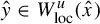 ,
$E^u_k(\hat y)$
 exists and is given by

In particular,
$E^u_k$
 is uniformly continuous along local unstable manifolds where it is defined. The analogous statement holds for
$E^s_k$
 with respect to
$H^s$
 holonomies.
Proof. We write the proof in the case of the stable bundle to avoid negative signs. The point is that for
$\hat {x}\in W^s_{\mathrm {loc}}(\hat {y})$
 , we have that

and
$H^s_{\sigma ^n(\hat {x})\sigma ^n(\hat {y})}\to \text {Id}$
 while the gaps between the singular values of
$A^n(\hat {x})$
 are growing arbitrarily large. Writing
$S_k(A)$
 for the span of the smallest k singular vectors of a matrix A, from (7) we have

By directly estimating the norm restricted to subspaces by using the angles between singular subspaces of
$A(\hat {x})$
 , one can deduce that
$S_k(H^s_{\sigma ^n(\hat {x})\sigma ^n(\hat {y})}A^n(\hat {x}))$
 converges to
$ E^s_k(\hat {x})$
 and
$S_k(A^n(\hat y)H^s_{\hat {x}\hat {y}})$
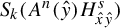 converges to
$H^s_{\hat {y}\hat {x}}(E^s_k(\hat {y}))$
 . Thus, by passing to the limit we find that

as desired.
2.2 Product structure of measures
We now describe continuous local product structure. For each
$1\le i\le m$
 , there exists the projection
$[0;i]\to \pi _s([0;i])\times \pi _u([0;i])$
 . For convenience, we will denote by
$\hat {\mu }^s_i,\hat {\mu }^u_i$
 these pushforwards of
$\hat {\mu }\vert _{[0;i]}$
 by
$\pi _s$
 and
$\pi _u$
 on the one-sided shifts. We say that
$\hat {\mu }$
 has continuous local product structure if for each symbol i there is a continuous function
$\psi \colon \hat {\Sigma }\to (0,\infty )$
 such that

Equation (8) is a description of the conditional measures on local stable and unstable leaves:

Note that local unstable holonomy between local stable sets has a bounded Jacobian for these conditional measures, where the bound is given by
$0<\max \psi /\min \psi <\infty $
 . In particular, from equation (9) we have the following description of the conditional measures along local stable sets. On the local stable set containing the point
$\hat {x} \in \hat {\Sigma }$
 , we then have a simple expression for the Radon–Nikodym derivative:

We now consider how the stable measures transform under application of the dynamics. Our goal is to show that we may arrange that the conditional measures along unstable leaves not become distorted at small scale as we iterate the dynamics forward. The precise statement is in Lemma 2.6.
The essence of the following proposition is that the conditional measures of
$\hat {\mu }$
 along stable and unstable leaves have a continuous Jacobian with respect to pushforward.
Proposition 2.4. [Reference ButlerBut18, Proposition 3.1]
There are continuous functions
$J_u\colon \Sigma ^u\to (0,\infty )$
 and
$J_s\colon \Sigma ^s\to (0,\infty )$
 such that for each
$1\le i,j\le l$
 and each Borel subset
${K_u\subseteq [0;i]^u}$
 ,

and likewise for each Borel subset
$K_s\subseteq [0;i]^s$
 .
In the following lemma, we consider the preimage of a local stable set
$W^s_{\mathrm {loc}}(\hat {x})$
 . This preimage may intersect several of the cylinders
$[0;i]$
 . For convenience, we write
$\hat {\mu }^s_{\hat {x},j}$
 for the conditional measure on
$\hat {\sigma }^{-1}(W^s_{\mathrm {loc}}(\hat {x})\cap [0;j])$
 .
Lemma 2.5. Suppose that
$\hat {\Sigma }$
 is a subshift of finite type as described above defined by a matrix M. We have the following formula for the invariance of the measure under the shift. There exists a positive continuous function
$J^u\colon \hat {\Sigma }\to \mathbb R^+$
 that is constant on local stable leaves such that we have the following product formula for the measure. For each i,

where the subscript in the sum indicates we are summing over all symbols j for which
$ji$
 is a subword permitted by M.
Proof. To begin, we have from Proposition 2.4 that for each
$\hat y\in [0;j,i]$
 there exists
$J^u_{ji}$
 such that

We now obtain a formula for the pushforward of
$\hat {\mu }\vert _{[0;j,i]}$
 . This measure may be written as

By pushing this forward by
$\hat {\sigma }$
 , we obtain an expression for the measure on
$[-1;j,i]\subseteq [0;i]$
 :

But from equation (10), this is the same as

Thus, summing over all symbols j that may precede i, we obtain the expression promised by the lemma.
The following fact is then straightforward to derive.
Lemma 2.6. Suppose that
$\hat {\Sigma }$
 is a shift and that
$\mu $
 is a
$\hat {\sigma }$
 -invariant probability measure on
$\hat {\Sigma }$
 with continuous product structure. Then the conditional measures satisfy the following property. If
$\hat {x}\in \hat {\Sigma }$
 and K is a subset of
$W^s_{\mathrm {loc}}(\hat {x})$
 then for all
$n\ge 0$
 we have that

Proof. Consider
$\hat {\sigma }^{-1}(W^s_{\mathrm {loc}}(\hat {x}))$
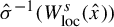 . Then there are points
$\hat y_1,\ldots ,\hat y_k$
 such that

From Lemma 2.5, because
$J^u$
 is constant along local stable leaves, it follows that there exist positive numbers
$\xi _i$
 ,
$1\le i\le k$
 , such that

By iterating on this formula we obtain the lemma.
2.3 Grassmannians, arrangements, and quasi-projective maps
Here we introduce the definitions related to Grassmannian cocycles necessary to study Lyapunov exponents with multiplicity
$1$
 . Throughout
$\Lambda ^p (\mathbb R^d)$
 denotes the space of alternating p-forms over
$\mathbb R^d$
 and
$\mathrm {Gr}(p,d)$
 the Grassmannian of p-dimensional subspaces, which includes
$\mathbb {P} \Lambda ^p(\mathbb R^d)$
 as the decomposable p-forms, that is, the p-forms
$\eta $
 which may be written as
$\eta = v_1 \wedge \cdots \wedge v_p$
 . In what follows we endow
$\mathrm {Gr}(k,d)$
 with the metric

Any
$\omega \in \Lambda ^{d-p}(\mathbb R^d)$
 defines a hyperplane
$H_{\omega } \subseteq \Lambda ^p(\mathbb R^d)$
 which is defined to be the kernel of the map
$\eta \mapsto \eta \wedge \omega $
 . When
$\omega $
 is defined by a decomposable
$(d-p)$
 -form, we think of
$\omega $
 as being ‘geometric’ because it defines a p-dimensional subspace of
$\mathbb R^d$
 . Hence, we may also define geometric hyperplanes in
$\Lambda ^p(\mathbb R^d)$
 . For a
$d-p$
 -form
$\omega $
 , the intersection of
$H_{\omega }$
 with
$\mathrm {Gr}(p,d)$
 is called a hyperplane section of
$\mathrm {Gr}(p,d)$
 . Hence, when a hyperplane section of
$\mathrm {Gr}(p,d)$
 is defined by a decomposable
$(d-p)$
 -form
$\omega $
 , we call it a geometric hyperplane section. We call a finite intersection of hyperplane sections a linear section of
$\mathrm {Gr}(p,d)$
 . In the case that a linear section of
$\mathrm {Gr}(p,d)$
 is defined by geometric hyperplane sections, we call it a geometric linear section. Finally, a finite union of linear sections is called a linear arrangement, and when we take a finite union of geometric linear sections, we call this a geometric linear arrangement. Similarly, one may define a geometric subspace of
$\Lambda ^p(\mathbb R^d)$
 as a finite intersection of geometric hyperplanes in
$\Lambda ^p(\mathbb R^d)$
 .
Observe that in
$\mathrm {Gr}(1,d)$
 linear sections are just subspaces of
$\mathbb R^d$
 . Linear arrangements play an analogous role in defining irreducibility conditions as the classic strong irreducibility condition does in Furstenberg’s theorem on positivity of the top Lyapunov exponent.
The following lemma shows that linear arrangements indeed carry some properties of finite unions of linear subspaces to higher Grassmannians.
Lemma 2.7. [Reference VianaVia14, Lemma 8.4]
If
$\{\mathcal {L}_\alpha : \alpha \in I\}$
 is an arbitrary family of linear arrangements in
$\mathrm {Gr}(p,d)$
 then
$\bigcap _\alpha \mathcal {L}_\alpha $
 coincides with the intersection of the
$\mathcal {L}_\alpha $
 over a finite family. Hence, the family of linear arrangements is closed under finite union and arbitrary intersections and, moreover, for
$B \in \mathrm {GL}(d)$
 the inclusion
$B(\mathcal {L}) \subseteq \mathcal {L}$
 implies that
$B(\mathcal {L}) = \mathcal {L}$
 .
The space of linear sections
$\mathcal {S} = \mathbb {P} S \cap \mathrm {Gr}(p,d)$
 , where S denotes a subspace of
$\Lambda ^p(\mathbb R^d)$
 , is topologized via the topology for linear subspaces of
$\Lambda ^p(\mathbb R^d)$
 . Namely, we say that
$\mathcal {S}_n \to \mathcal {S}$
 if and only if
$S_n \to S$
 .
In [Reference VianaVia14, Ch. 8], it is claimed that the space of geometric linear sections is compact in order to prove simplicity of spectrum under a version of twisting and pinching. However, as we see in Example 2.8 below, there seems to be an oversight in this claim. Because of this we state irreducibility criteria in terms of linear sections that are not necessarily geometric.
The dimension of a linear section
$\mathcal {S} = \mathbb {P} S \cap \mathrm {Gr}(p,d)$
 is defined simply as the dimension of S as a subspace of
$\Lambda ^p (\mathbb R^d)$
 . Once we remove the geometric restriction, we regain compactness of the space of linear sections of a fixed dimension.
Example 2.8. In this example, we show that if
$D_n$
 is a sequence of geometric linear sections of a Grassmannian, then
$\lim _n D_n$
 is not necessarily a geometric linear section: it is still a linear section, but it may no longer be geometric. We construct our example in
$\mathrm {Gr}(2,4)$
 .
Let
$\eta = e_1 \wedge e_2 \in \Lambda ^2 (\mathbb R^4)$
 and
$\omega _n = (e_1 + n^{-1}e_3) \wedge (e_2 + n^{-1}e_4) \in \Lambda ^2 (\mathbb R^4)$
 . We will write
$e_{ij} := e_i \wedge e_j$
 . Then
$H_\eta $
 and
$H_{\omega _n}$
 , the hyperplane sections defined by
$\eta $
 and
$\omega _n$
 respectively, are

Thus,

is by definition a sequence of geometric linear sections when intersected with
$\mathrm {Gr}(2,4)$
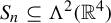
 . Write
$D_n=S_n\cap \mathrm {Gr}(2,4)$
 , which may be identified with the decomposable tensors
${S_n\subseteq \Lambda ^2(\mathbb R^4)}$
 . We claim that
$D=\lim _{n} D_n$
 is not a geometric linear section of
$\mathrm {Gr}(2,4)$
 .
To see this we will first find a description of what D is, then we will show that D cannot be geometric because any decomposable
$1$
 -form vanishing when wedged with all elements of D is a multiple of
$e_{12}$
 .
To proceed we use that
$\omega \in \Lambda ^2(\mathbb R^4)$
 is decomposable if and only if
$\omega ^2=0$
 . By doing so we may calculate which tensors in
$S_n$
 are decomposable. Namely, we see that

if and only if
$d^2+adn^{-1}-bc=0$
 .
If we let
$S=\lim _n S_n$
 then

In particular, if we calculate as before, we see that
$S\cap \mathrm {Gr}(2,4)$
 is equal to the tensors of the form

with
$d^2-bc=0$
 . Thus, by comparing pointwise limits for different values of
$a,b,c,d$
 , we find that
$D=S\cap \mathrm {Gr}(2,4)$
 . In particular, note that some of the forms in D are
$e_{12},e_{13},e_{24}$
 and
$(e_1+e_2)\wedge (e_3+e_4)$
 . Thus, any
$\omega \in \Lambda ^2(\mathbb R^4)$
 that vanishes when wedged with things in D must be of the form

which is decomposable if and only if
$bc=0$
 . In the cases that
$a\neq 0$
 and
$b=0$
 , the form we get is a multiple of
$e_2\wedge (e_1+ce:3)$
 , which does not vanish when wedged with
${(e_1+e_2)\wedge (e_3+e_4)}$
 unless
$c=0$
 . So, the form must be
$e_{12}$
 . Similarly, if
$c=0$
 , the form is a multiple of
$e_1\wedge (e_2+be_4)$
 and we must have
$b=0$
 as before. Thus, if
$a\neq 0$
 , the only forms we get are multiples of
$e_{12}$
 . If
$a=0$
 , then we get
$e_{14}$
 and
$e_{23}$
 neither of which vanish when wedged with
$(e_1+e_2)\wedge (e_3+e_4)$
 . Thus, the only decomposable forms vanishing when wedged with everything in D are multiples of
$e_{12}$
 .
But this means that D cannot be a geometric linear section of
$\mathrm {Gr}(2,4)$
 because it is not defined by
$H_{e_{12}}$
 . Therefore the space of geometric linear sections is not compact.
When passing to the limit of the actions of linear maps on Grassmannians, it is useful to work with quasi-projective maps. We recall some definitions below.
If
$P\in \mathrm {GL}(d,\mathbb R)$
 is a linear map then it induces a map
$P_{\#}\colon \mathrm {Gr}(k,d)\to \mathrm {Gr}(k,d)$
 for each
$1\le k \le d$
 . We call such maps projective and often we denote the action of P on Grassmannians simply by P when there is no ambiguity.
The space of projective maps on
$\mathrm {Gr}(k,d)$
 admits a very useful natural compactification which we now describe. Recall that we may embed
$\mathrm {Gr}(k,d)$
 in
$\mathbb {P} \Lambda ^k(\mathbb R^d)$
 , so the space of projective maps of
$\mathrm {Gr}(k,d)$
 embeds into the space of linear maps of
$\Lambda ^k(\mathbb R^d)$
 with norm 1 with respect to the natural norm of
$\Lambda ^k(\mathbb R^d)$
 . Since the latter is clearly compact, the closure of the set of projective maps regarded as above must also be, and its elements are referred to as quasi-projective maps. For more details of this construction, we refer the reader to [Reference Avila and VianaAV07a, §2.1].
A quasi-projective map Q has a well-defined kernel when regarded as a linear map on
$\Lambda ^k(\mathbb R^d)$
 . We define
$\ker Q \subseteq \mathrm {Gr}(k,d)$
 to be the intersection of its kernel as a linear map on
$\Lambda ^k(\mathbb R^d)$
 with
$\mathrm {Gr}(k,d)$
 , again using the embedding of
$\mathrm {Gr}(k,d)$
 in
$\mathbb {P} \Lambda ^k(\mathbb R^d)$
 . Since linear maps of the form
$\Lambda ^k P$
 map rank 1 tensors to rank 1 tensors in
$\Lambda ^k(\mathbb R^d)$
 and the space of rank 1 tensors is compact in
$\mathbb {P}\Lambda ^k(\mathbb R^d)$
 , for
$\xi \in \mathrm {Gr}(k,d) \setminus \ker Q$
 , we may define
${Q(\xi ) \in \mathrm {Gr}(k,d)}$
 using the corresponding action of Q on
$\mathbb {P} \Lambda ^k(\mathbb R^d)$
 . Hence, quasi-projective maps can be regarded as functions
$Q: \mathrm {Gr}(k,d) \setminus \ker Q \to \mathrm {Gr}(k,d)$
 .
Lemma 2.9. [Reference Avila and VianaAV07a, Lemma 2.3]
The kernel of any quasi-projective map Q on
$\mathrm {Gr}(k,d)$
 is contained in some hyperplane section of
$\mathrm {Gr}(k,d)$
 .
For a measure
$\nu $
 on
$\mathrm {Gr}(k,d)$
 , the pushforward measure
$Q_* \nu $
 is well defined as long as
$\nu (\ker Q) = 0$
 . The following lemma will be very useful in our proof.
Lemma 2.10. [Reference Avila and VianaAV07a, Lemma 2.4]
If
$(P_n)$
 is a sequence of projective maps converging to some quasi-projective map Q of
$\mathrm {Gr}(k,d)$
 and
$(\nu _n)$
 is a sequence of probability measures in
$\mathrm {Gr}(k,d)$
 converging weakly to some probability
$\nu $
 with
$\nu (\ker Q)=0$
 then
$(P_n)_*\nu _n$
 converges weakly to
$Q_*\nu $
 .
2.4 Invariant u-states
The cocycle
$\hat {A}$
 induces a cocycle on the Grassmannian bundle
$\hat {\Sigma }\times \mathrm {Gr}(k,d)$
 in the natural way, which by abuse of notation we also denote by
$\hat {A}$
 . Similarly, the stable and unstable holonomies induce maps on the Grassmannians which we denote by the same symbols.
Definition 2.11. For a fiber-bunched cocycle
$\hat {A}\colon \hat {\Sigma } \to \mathrm {GL}(d,\mathbb R)$
 and a shift-invariant measure
$\hat {\mu }$
 on
$\hat {\Sigma }$
 , we say that a probability measure
$\hat {m}$
 on
$\hat {\Sigma } \times \mathrm {Gr}(k,d)$
 is a u-state over
$\hat {\mu }$
 if it is invariant by the cocycle and

for any
$\hat {x}$
 and
$\hat y$
 in the same local unstable leaf, and where
$\{\hat {m}_{\hat {x}} : \hat {x} \in \hat {\Sigma }\}$
 is a family of measures on
$\mathrm {Gr}(k,d)$
 given by the disintegration of
$\hat {m}$
 along the partition
$\{\{\hat {x}\} \times \mathrm {Gr}(k,d): \hat {x} \in \hat {\Sigma }\}$
 .
When
$\hat {\mu }$
 has continuous local product structure, u-states have several other useful properties. We assume that
$\hat {A}$
 is a fiber-bunched cocycle and
$\hat {\mu }$
 is a measure with continuous local product structure. The following propositions from [Reference Avila and VianaAV07a] sum up the relevant properties about u-states used in our proof.
Proposition 2.12. [Reference Avila and VianaAV07a, Proposition 4.2]
There exists a u-state
$\hat {m}$
 on
$\mathrm {Gr}(k,d)$
 .
The projection m of an invariant measure
$\hat {m}$
 on
$\hat {\Sigma } \times \mathrm {Gr}(k,d)$
 to
$\Sigma \times \mathrm {Gr}(k,d)$
 similarly admits a disintegration over the fibers
$\{x\} \times \mathrm {Gr}(k,d)$
 , which we denote by
$\{m_x : x \in \Sigma \}$
 . A martingale convergence argument relates
$\hat {m}_{\hat {x}}$
 to
$m_x$
 for any invariant measure (not necessarily a u-state).
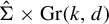
Proposition 2.13. [Reference Avila and VianaAV07a, Corollary 3.4]
Let
$\hat {m}$
 be an invariant probability measure on
$\hat {\Sigma } \times \mathrm {Gr}(k,d)$
 which projects to
$\hat {\mu }$
 . For
$\hat {\mu }$
 -a.e.
$\hat {x} \in \hat {\Sigma }$
 ,

where the limit is taken in the weak* topology, and P is the projection onto the one-sided shift
$\Sigma ^u$
 as before.
Moreover, the following result also holds for any m, not necessarily a u-state:
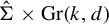
Lemma 2.14. [Reference Avila and VianaAV07a, Lemma 4.5]
Let
$\hat {m}$
 be an invariant probability measure on
${\hat {\Sigma } \times \mathrm {Gr}(k,d)}$
 which projects to
$\hat {\mu }$
 . Then the measures
$\{m_x: x \in \Sigma \}$
 given by

define a disintegration of m along
$\{\{x\} \times \mathrm {Gr}(k,d): x \in \Sigma \}.$

When m is a u-state, the lemma above and invariance by unstable holonomies additionally give continuity of the disintegration
$\{m_x: x \in \Sigma \}$
 .
Proposition 2.15. [Reference Avila and VianaAV07a, Proposition 4.4]
Any u-state m on
$\Sigma \times \mathrm {Gr}(k,d)$
 admits some disintegration
$\{m_x : x \in \Sigma \}$
 into measures on
$\mathrm {Gr}(k,d)$
 which vary weak* continuously with respect to x.
Lastly, using the continuity property above, one also obtains the following invariance statement for the disintegration
$m_x$
 .
Proposition 2.16. [Reference Avila and VianaAV07a, Corollary 4.7]
If m is a u-state and
$m_x$
 is the continuous disintegration of m from Lemma 2.14, then

for every
$x \in \Sigma $
 and
$k \geq 1$
 , and
$J\sigma ^k$
 is a bounded measurable function for each
$k \geq 1$
 .
3 Strong irreducibility and distribution of Oseledec subspaces
The first key step in the proof of Furstenberg’s theorem and in the main theorem in [Reference Avila and VianaAV07a] is using an irreducibility hypothesis to prove that the measure of u-states disintegrated over the one-sided shift cannot be concentrated on subspaces. We prove the corresponding result in our setting in Proposition 3.3. For the rest of the paper we fix a fiber-bunched cocycle
$\hat {A}:\hat {\Sigma } \to \mathrm {GL}(d, \mathbb R)$
 .
Definition 3.1. A function
$\mathcal {L}$
 from a topological space X to the set of linear arrangements in
$\mathrm {Gr}(k,d)$
 is said to be a continuous family of k-linear arrangements on X if there is an
$n \in {\mathbb N}$
 such that for each
$x \in X$
 ,

where each
$\mathcal {S}_i(x)$
 is of the form
$\mathbb {P} S_i(x) \cap \mathrm {Gr}(k,d)$
 and the
$S_i$
 are continuous functions from X to the space of linear subspaces of
$\Lambda ^k(\mathbb R^d)$
 of a fixed dimension
$d(i)$
 . The continuous family of linear arrangements is said to be non-trivial if
$\mathcal {L}(x)$
 is neither all of
$\mathrm {Gr}(k,d)$
 nor the empty set for all
$x \in X$
 .
Definition 3.2. A continuous cocycle
$\hat {A}\colon \hat {\Sigma } \to \mathrm {GL}(d, \mathbb R)$
 is strongly reducible on
$\mathrm {Gr}(k,d)$
 if there exists a non-trivial continuous family of k-linear arrangements
$\mathcal {L}$
 on
$\hat {\Sigma }$
 invariant by
$\hat {A}$
 , that is, for every
$\hat {x} \in \hat {\Sigma }$
 :

The cocycle
$\hat {A}$
 is strongly irreducible on
$\mathrm {Gr}(k,d)$
 if it is not strongly reducible on
$\mathrm {Gr}(k,d)$
 . The cocycle is said to be fully irreducible if it is strongly irreducible on
$\mathrm {Gr}(k,d)$
 for all
$1 \leq k \leq d-1$
 .
Fix a shift-invariant measure
$\hat {\mu }$
 on
$\hat {\Sigma }$
 with continuous local product structure. The following key proposition shows that u-states of fully irreducible fiber-bunched cocycles on Grassmannians must be smooth in a certain sense.
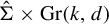
Proposition 3.3. Suppose
$\hat {A}$
 is strongly irreducible on
$\mathrm {Gr}(k,d)$
 . Let
$\hat {m}$
 be a u-state on
$\hat {\Sigma } \times \mathrm {Gr}(k,d)$
 associated to
$\hat {\mu }$
 . For
$x \in \Sigma $
 , let
$\{m_x\}_{x\in \Sigma }$
 be the disintegration of m over the fibers of
$\Sigma \times \mathrm {Gr}(k,d)$
 . Then
$m_x(\mathcal {S}) = 0$
 for every
$x \in \Sigma $
 and any linear section
$\mathcal {S}$
 of
$\mathrm {Gr}(k,d)$
 . In particular,
$m_x(H) = 0$
 for every
$x \in \Sigma $
 and any hyperplane section H of
$\mathrm {Gr}(k,d)$
 .
To begin the proof we prove that we can reduce the problem to the reduced cocycle from equation (5) and the one-sided shift. Note that because the reduced cocycle is constant on local stable leaves, it defines a cocycle over the one-sided shift
$\Sigma $
 .
Proposition 3.4. For every
$1 \leq k \leq d$
 , there does not exist a non-trivial continuous family
$\mathcal {L}$
 of k-linear arrangements on
$\Sigma $
 invariant by the cocycle on the one-sided shift induced by the reduced cocycle from equation (5).
Proof. Indeed, if there were such a
$\mathcal {L}$
 , then, using the definition of
$\phi ^u$
 appearing before equation (5), we could define
$\hat {\mathcal {L}}(\hat {x})$
 on
$\hat {\Sigma }$
 by
$ \hat {\mathcal {L}}(\hat {x}) = H^s_{\phi ^u(\hat {x}), \hat {x}} \mathcal {L}(x)$
 so that

which yields invariance of
$\hat {\mathcal {L}}$
 . Moreover, since stable holonomies are continuous in the leaf and transverse direction, continuity of
$\hat {\mathcal {L}}$
 follows from continuity of
$\mathcal {L}$
 .
As
$\hat {A}$
 is by definition conjugate to A, for the goal of proving simplicity of spectrum it suffices to work with A. Hence, from now on we work only with the reduced cocycle A.
Proof of Proposition 3.3.
We take the continuous disintegration of m from Lemma 2.14. Suppose that
$m_x(\mathcal {S})> 0$
 for some
$x \in \Sigma $
 and some linear section
$\mathcal {S}$
 of
$\mathrm {Gr}(k,d)$
 . Let
$d_0$
 be the minimal dimension such that there exists a subspace S of
$\Lambda ^k(\mathbb R^d)$
 such that
$m_x(\mathbb {P} S \cap \mathrm {Gr}(k,d))> 0 $
 for some
$x \in \Sigma $
 . Let

We claim that by compactness
$\gamma _0$
 is realized. The space of all
$\mathbb {P}S$
 is compact and
$m_x$
 varies continuously in x in the weak* topology by Proposition 2.15. Hence, if we take any sequence
$x_i, S_i$
 such that

we may pass to a subsequence so that we may assume that
$x_i\to x'$
 and
$S_i\to S$
 . Consider the set
$B_{\epsilon }(S)$
 ; then weak* convergence implies that for each
$\epsilon $
 as
$B_{\epsilon }(S)$
 is closed,

Letting
$\epsilon \to 0$
 , we obtain that
$m_{x'}(\mathbb {P}S\cap \mathrm {Gr}(k,d))=\gamma _0$
 by continuity from above of the measures.
We now claim that for each
$x \in \Sigma $
 , there exists at least one subspace
$S(x)$
 of dimension
$d_0$
 such that
$m_x(S(x) \cap \mathrm {Gr}(k,d)) = \gamma _0$
 . The proof is along the same lines as in [Reference Avila and VianaAV07a, Lemma 5.2]. First, one shows that over every cylinder
$[J]$
 the supremum of
$m_x(S\cap \mathrm {Gr}(k,d))$
 is
$\gamma _0$
 . Then one can pick a sequence converging to any point
$x'\in \Sigma $
 as above. We are able to pass to this limit because the space of linear sections is compact.
We now show that the linear sections realizing the supremum form a continuous family. First, we show that there exists
$\ell $
 such that at every point
$x\in \Sigma $
 there exist exactly
$\ell $
 distinct linear
$d_0$
 -dimensional subspaces of
$\Lambda ^k(\mathbb R^d)$
 ,
$S_1(x),\ldots , S_{\ell }(x)$
 such that
$m_x(\mathbb {P} S_i(x) \cap \mathrm {Gr}(k,d))=\gamma _0$
 . Take a point
$x\in \Sigma $
 that maximizes the number
$\ell $
 . Then by invariance of
$m_x$
 (that is, Proposition 2.16),

it follows for each
$z\in \sigma ^{-k}(x)$
 that

Note that the preimages of x become dense in
$\Sigma $
 . Thus, for any point
$q\in \Sigma $
 , we may take a sequence of
$z_n$
 such that
$z_n\to q$
 and
$m_{z_n}$
 gives measure
$\gamma _0$
 to exactly
$\ell $
 subspaces
$S_1(z_n),\ldots , S_\ell (z_n)$
 . By the argument mentioned after equation (11), we may pass to a subsequence so that, for each i,
$S_i(z_n)\to S_i'$
 , where
$S_i'$
 are
$d_0$
 -dimensional subspaces of
$\Lambda ^k(\mathbb R^d)$
 . We claim that all the
$S_i'$
 are distinct. But this is clear: if two coincided, then the preceding argument implies that the limiting measure of some
$S_i'$
 would be at least
$2\gamma _0$
 , which is impossible as
$\gamma _0$
 is the maximum.
Now we show that these sections vary continuously as x varies. First observe that if
$x_n\to x$
 then for each n we must have that
$S_i(x_n)$
 is near some
$S_j(x)$
 ; otherwise, by taking a limit as before, we would obtain an additional section
$S'$
 of measure
$\gamma _0$
 for
$m_x$
 .
Finally, to see that the family
$\{S_1(x),\ldots , S_\ell (x)\}_{x\in \Sigma }$
 is invariant under the cocycle, note that this holds on the set of pre-images of z and that this set is dense. Thus, invariance holds by continuity. But we have now reached a contradiction to our assumption of irreducibility on
$\mathrm {Gr}(k,d)$
 , so we are done.
3.1 Distribution of Oseledec subspaces
If we know a priori that for
$\hat {\mu }$
 we have
$\unicode{x3bb} _{k}(\hat {\mu })> \unicode{x3bb} _{k+1}(\hat {\mu })$
 then u-states over
$\hat {\mu }$
 are supported on
$E^u_k$
 . The following proposition makes this precise.
Proposition 3.5. Suppose
$\hat {\mu }$
 has full support and continuous local product structure and
$\unicode{x3bb} _{k}(\hat {\mu })> \unicode{x3bb} _{k+1}(\hat {\mu })$
 . Let
$\hat {m}$
 be any u-state of
$\hat {\mu }$
 on
$\hat {\Sigma } \times \mathrm {Gr}(k, d)$
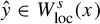
 . Then for any
$x \in \Sigma $
 and
$\hat {\mu }^s_x$
 -a.e.
$\hat y \in W^s_{\mathrm {loc}}(x)$
 ,

Proof. Recall that by Proposition 2.13, for
$\hat {\mu }$
 -a.e.
$\hat {x} \in \hat {\Sigma }$
 ,

where
$P\colon \hat {\Sigma } \to \Sigma $
 is the projection from the two-sided to the one-sided shift.
Passing to a subsequence
$n_j$
 such that
$\hat {\sigma }^{-n_j}(\hat {x}) \to \hat {x}_0$
 , since
$x \mapsto m_x$
 is weak
$*$
 continuous,

where, as usual,
$x_0 = P(\hat {x}_0)$
 . Moreover, by passing to a further subsequence if needed, since the space of quasi-projective maps is compact we may assume that
$A^{n_j}(\hat {\sigma }^{-n_j}(\hat {x}))$
 converges to some quasi-projective map
$Q_0$
 . By the Oseledec theorem, since
$\unicode{x3bb} _{k}(\hat {\mu })> \unicode{x3bb} _{k+1}(\hat {\mu })$
 , the sequence of maps
$A^n(\hat {\sigma }^{-n}(\hat {x}))$
 has

for
$\hat {\mu }$
 -a.e.
$\hat {x}$
 , so the image of
$Q_0$
 in
$\mathrm {Gr}(k,d)$
 must be the single point in
$\mathrm {Gr}(k,d)$
 given by

again by the Oseledec theorem. Finally, since by Proposition 3.3 and Lemma 2.9
$m_{x_0}(\ker Q_0) = 0$
 , we apply Lemma 2.10 to conclude that

holds for
$\hat {\mu }$
 -a.e.
$\hat {x}$
 . In particular, by the disintegration formula, for
$\mu $
 -a.e.
$x \in \Sigma $
 the statement must hold for
$\hat {\mu }^s_x$
 -a.e.
$\hat y \in W^s_{\mathrm {loc}}(x)$
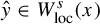 .
Now we want to upgrade this statement to every
$x \in \Sigma $
 . Fix some
$x_0\in \Sigma $
 for which the statement holds for
$\hat {\mu }^s_{x_0}$
 -a.e.
$\hat y \in W^s_{\mathrm {loc}}(x_0)$
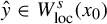 and fix an arbitrary
$x \in \Sigma $
 which lies in the same
$[0:i]$
 cylinder. Because
$\hat {m}$
 is a u-state, for
$\hat y \in W^s_{\mathrm {loc}}(x_0)$
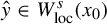 and
$\hat z = W^u_{\mathrm {loc}}(\hat y) \cap W^s_{\mathrm {loc}}(x)$
 ,

so that
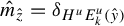
$\hat {m}_{\hat z} = \delta _{H^uE^u_k(\hat y)}$
 for
$\hat {\mu }^s_{x_0}$
 -a.e.
$\hat y \in W^s_{\mathrm {loc}}(x_0)$
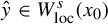 , since the measures
$\hat {\mu }^s_{x_0}$
 and
$\hat {\mu }^s_{x}$
 are equivalent due to the continuous product structure. But since
$H^u_{\hat y \hat z} E^u_k(\hat y) = E^u(\hat z)$
 by Lemma 2.3 and there are only finitely many cylinders
$[0:i]$
 , the proof is complete.
Remark 3.6. It is natural to consider if the correct definition of strong irreducibility for cocycles admitting invariant holonomies should be weakened by requiring non-existence of a continuous family
$\mathcal {L}$
 which is in addition invariant by the holonomies. However, in [Reference Gouezel and StoyanovGS19, Remark 3.11] the authors show that with this weaker definition, which they call holonomy irreducibility, the conditional measures of u-states do not have to lie on a single Dirac mass, so Proposition 3.5 does not hold. Their example suggests that in the study of cocycles admitting canonical holonomies it is more natural not to include invariance by holonomies in the definition of irreducibility.
Remark 3.7. Since the conjugacy between the unreduced and reduced cocycles preserves the unstable directions and conjugates the stable holonomies to the identity, if we consider instead the unreduced cocycle
$\hat {A}$
 , the statement of Proposition 3.3 may still be interpreted as saying that given any hyperplane section H of
$\mathrm {Gr}(k,d)$
 , any
$\hat {x} \in \hat {\Sigma }$
 then for
$\hat {\mu }^s_x$
 -a.e. point
$\hat y$
 in
$W^s_{\mathrm {loc}}(\hat {x})$
 the conditional measure
$\hat {m}_{\hat y}$
 gives
$0$
 measure to
$H^s_{\hat {x} \hat y}H$
 . In particular, if
$\hat {\mu }$
 has
$\unicode{x3bb} _k(\hat {\mu })> \unicode{x3bb} _{k+1}(\hat {\mu })$
 , we have
$\hat {m}_{\hat y} = \delta _{E^u_k(\hat y)}$
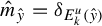 for
$\hat {\mu }$
 -a.e.
$\hat y$
 by the preceding proposition, so that for every
$\hat {x} \in \hat {\Sigma }$
 and
$\hat {\mu }^s_{\hat {x}}$
 -a.e. point
$\hat y$
 in
$W^s_{\mathrm {loc}}(\hat {x})$
 one must have
$E^u_k(\hat y) \notin H^s_{\hat {x} \hat y}H$
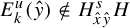 for the unreduced cocycle.
Similarly, the analogous statement holds for the stable directions along an unstable manifold, that is, for a fixed hyperplane section
$H \subseteq \mathrm {Gr}(d-k, d)$
 and a fixed
$\hat {x} \in \hat {\Sigma }$
 , for
$\hat {\mu }^u_{\hat {x}}$
 -a.e. point
$\hat y$
 in
$W^u_{\mathrm {loc}}(\hat {x})$
 the statement
$E^s_{d-k}(\hat y) \notin H^u_{\hat {x} \hat y}H$
 holds.
4 Convergence to a Dirac measure
Now we turn to the proof of Theorem B. Throughout, we fix
$1 \leq k \leq d-1$
 and
$\hat {\mu }$
 and
$\hat \eta $
 as in the statement of Theorem B. The key step to obtain
$\unicode{x3bb} _k(\hat \eta )> \unicode{x3bb} _{k+1}(\hat \eta )$
 is to prove that for u-states of
$\hat {\eta }$
 the conditional measures on
$\mathrm {Gr}(k,d)$
 are Dirac measures.
Proposition 4.1. Let
$\hat {m}^\eta $
 be an invariant u-state for
$\hat \eta $
 on
$\hat {\Sigma } \times \mathrm {Gr}(k, d)$
 . Then for
$\hat \eta $
 -a.e.
$\hat {x}$
 , the conditional measure
$\hat {m}^{\eta }_{\hat {x}}$
 is a Dirac delta on
$\mathrm {Gr}(k, d)$
 . That is, there exists some
$\xi ^u(\hat {x}) \in \mathrm {Gr}(k, d)$
 such that

We give the proof of Proposition 4.1 at the end of this section. The existing approaches showing that cocycles have non-trivial Lyapunov exponents all rely on some form of ‘twisting’ and ‘pinching’. The approach we take to show the convergence to Dirac measures is similar to preexisting ones: we assume a form of pinching and twisting. Our pinching assumption is the existence some other ergodic fully supported measure
$\hat {\mu }$
 with continuous local product structure and
$\unicode{x3bb} _{k}(\hat {\mu })> \unicode{x3bb} _{k+1}(\hat {\mu })$
 , as in Theorem B. To construct a twisting setup in our setting we employ a novel approach using strong irreducibility (§3) combined with the behavior of generic orbits for
$\hat {\mu }$
 . We then conclude the proof in §5.
To begin the construction we fix a periodic point in
$\hat {\Sigma }$
 with an exponent gap which we will use to separate the exponents of generic orbits via shadowing. Since
$\unicode{x3bb} _{k}(\hat {\mu })>\unicode{x3bb} _{k+1}(\hat {\mu })$
 by the periodic approximation theorem [Reference KalininKal11, Theorem 1.4] there exists some periodic point
$\hat {p} \in \hat {\Sigma }$
 , such that the Lyapunov spectrum of A over the orbit of
$\hat {p}$
 is arbitrarily close to the Lyapunov spectrum of A with respect to
$\hat {\mu }$
 . Hence, we may take
$\hat p$
 so that the kth eigenvalue of
$A^q(\hat p)$
 , where q is the period o
$\hat p$
 , is greater than the
$(k+1)$
 th eigenvalue. Without loss of generality we will assume that
$\hat p$
 is a fixed point, that is,
$q=1$
 and
$\hat p$
 will be fixed for the rest of this section.
For the twisting construction, we will adopt the following notation. For
$\hat {x} \in \hat {\Sigma }$
 we define the unstable and stable cylinders
$C^{u,s}_{l}(\hat {x})$
 and the rectangle
$R_l(\hat {x})$
 of depth l at
$\hat {x}$
 , which is the ball of radius
$2^{-l}$
 at
$\hat {x}$
 , by

Observe that if
$\hat {x} \in [0:i]$
 , then
$R_0(\hat {x}) =[0:i]$
 by definition. Since k is fixed we will simply take
$\mathrm {Gr}$
 ,
$E^u$
 and
$E^s$
 to mean
$\mathrm {Gr}(k, d)$
 ,
$E^u_{k}$
 and
$E^s_{d-k}$
 , respectively. We will also use the following simple linear algebra lemma in the proof, where the angle
$\angle (V,W)$
 between two subspaces
$V,W$
 not necessarily of the same dimension is defined simply as the smallest angle between a vector in V and a vector in W.
Lemma 4.2. Fix
$d \geq 1$
 . Given
$\theta , \gamma> 0$
 , there is a
$K> 1$
 with the following property. Let
$A \in \mathrm {GL}(d,\mathbb R)$
 satisfy
$\sigma _k(A)> K \sigma _{k+1}(A)$
 . Then for any U of dimension k such that
$\angle ( U,S_{d-k}(A))> \theta $
 , one has

Moreover, A acts
$\gamma $
 -Lipschitz in the set of U such that
$\angle ( U,S_{d-k}(A))> \theta $
 in the Grassmannian.
Proof. By the singular value decomposition, this reduces to the analogous claim for diagonal matrices, which is straightforward because every unit vector
$Av$
 uniformly transverse to
$S_{d-k}$
 has the length of its
$U_k(A)$
 component uniformly bounded below.
In the following sequence of lemmas, we construct a sequence of rectangles such that points in the rectangles shadow
$\hat p$
 under
$\hat {\sigma }^{-1}$
 and such that under
$\hat {\sigma }$
 the cocycle over the points moves the direction expanded by shadowing
$\hat p$
 in the past away from fixed hyperplane sections, which will serve as ‘twisting’ orbits. We start with the construction of one of these rectangles in Lemma 4.3 and conclude the construction in Proposition 4.5.
Constructing
$\hat {q}$
 and
$R_{\rho }(\hat {q})$
 .

Figure 1 Long description
The diagram consists of two main regions. On the left, a Cartesian coordinate system is centered at a point p-hat. The vertical axis is labeled W sub loc super s of p-hat and the horizontal axis is labeled W sub loc super u of p-hat. A horizontal band defined by dashed lines is centered on the horizontal axis, labeled on the right with a bracket as C sub 2 l super u of p-hat. Inside this band is a series of vertical gray stripes of varying widths, identified by a legend at the bottom as a gray circle equals G sub l. A small dark gray rectangle intersects one of these stripes is the source of a curved arrow labeled sigma-hat super k. This arrow points to a dark gray square in the top-right corner labeled R sub rho of q-hat, which contains a central point q-hat.
From now on, for every point
$\hat {x} \in \hat {\Sigma }$
 , we will use superscripts to denote preimages under
$\hat {\sigma }$
 , for example
$\hat {x}^n = \hat {\sigma }^{-n}(\hat {x})$
 . (Recall that subscripts already denote the ith symbol of a word.) Moreover, observe in the following proofs that because we have taken the cocycle to be constant along local stable manifolds,
$A^n(\hat {y})=A^n(\hat {z})$
 for
$\hat z \in W^s_{\mathrm {loc}}(\hat y)$
 . See Figure 1 for an illustration of the the sets and points in the proof of Lemma 4.3.
Lemma 4.3. Fix some sufficiently small
$\theta _0>0$
 and let
$\hat {p}\in \hat {\Sigma }$
 . Suppose that
$\hat {q}$
 is Oseledec regular and generic for
$\hat {\mu }$
 . Then for all
$\epsilon>0$
 and
$l\in {\mathbb N}$
 , there exist
$\rho $
 and k such that the following assertions hold:
-
(1) $\hat {\sigma }^{-k}(R_{\rho }(\hat {q}))\subseteq C^u_l(\hat {p})$
; -
(2) for any $\hat {y}\in \hat {\sigma }^{-k}(R_{\rho }(\hat {q}))$
which is Oseledec regular, let
$\hat {z}=[\hat {y},\hat {p}]$
; then $$ \begin{align*} d_{Gr(k,d)}(A^k(\hat{y})E^u(\hat{z}),E^u(\hat{q}))<\epsilon; \end{align*} $$
-
(3) further, for $\hat y$
and
$\hat z$
as above,
$A^k(\hat {y})\colon \mathrm {Gr}(k,d)\to \mathrm {Gr}(k,d)$
is
$\gamma $
-Lipschitz on a
$\theta _0$
-neighborhood of
$E^u(\hat {z})$
.







Proof. We begin with the following claim.
Claim 4.4. For every
$\theta _0$
 sufficiently small and any
$l> 0$
 , there exists a measurable set
$G_l\subseteq C^u_{2l}(\hat {p})$
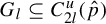 with the following properties:
-
(1′) $G_l$
has positive
$\hat {\mu }$
measure; -
(2′) for $\hat {y}\in G_l$
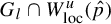
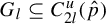
which is Oseledec regular, $$ \begin{align*} \angle (E^u(\hat z), E^s(\hat y))> 2 \theta_0, \quad\text{where }\hat z = [\hat{p},\hat{y}]; \end{align*} $$
-
(3′) $G_l$
is saturated by
$W^s_{\mathrm {loc}}$
-leaves in
$C^u_{2l}(\hat {p})$
; that is, for
$\hat {x} \in G_l$
, if
$\hat z \in W^s_{\mathrm {loc}}(\hat {x}) \cap C^u_{2l}(\hat p)$
, then
$\hat z \in G_l$
; -
(4′) for $\hat y \in G_l$
which is Oseledec regular the sequence of subspaces
$(S(\hat y, n))_n$
defined in §2.1 converges uniformly to
$E^s(\hat y)$
.


Proof. Let
$G_l$
 be the set of points in
$C^u_{2l}(\hat p)$
 which are Oseledec regular and satisfy condition (2
$^\prime $
 ). For
$y \in G_l$
 let
$\hat z = [\hat p,\hat y ]$
 . Since
$E^u(\hat z) = H^u_{\hat p, \hat z}E^u(\hat p)$
 , by Remark 3.7 applied for
$E^s$
 and H the hyperplane section defined by
$E^u(\hat p)$
 on
$\mathrm {Gr}(d-k,d)$
 , we see that, for all
$\theta _0$
 sufficiently small,
$G_l \cap W^u_{\mathrm {loc}}(\hat p)$
 has positive
$\hat {\mu }^u_{\hat p}$
 -measure. Observe that how much we need to shrink
$\theta _0$
 does not depend on l. Because
$E^s$
 is constant along
$W^s_{\mathrm {loc}}$
 -leaves,
$G_l$
 is saturated by
$W^s_{\mathrm {loc}}$
 -leaves in
$C^u_{2l}(\hat p)$
 , giving (3
$^\prime $
 ). Moreover, since
$\hat {\mu }$
 has a local product structure
$G_l$
 is a set of positive
$\hat {\mu }$
 -measure, so we have verified (1
$^\prime $
 ).
By restricting
$G_l$
 to a subset of positive
$\hat {\mu }$
 -measure we may assume by Egorov’s theorem that for
$\hat y \in G_l$
 the sequence of subspaces
$(S(\hat y, n))_n$
 converges uniformly to
$E^s(\hat y)$
 , verifying (4
$^\prime $
 ). Observe that since the cocycle is constant along local stable leaves, passing to this subset of positive measure does not affect the saturation by
$W^s_{\mathrm {loc}}$
 -leaves in
$C^u_{2l}(\hat p)$
 , that is, passing to this subset (3
$^\prime $
 ) still holds, so we are done.
Now we return to the proof of Lemma 4.3. Because
$\hat {q}$
 is generic for
$\hat {\mu }$
 and by (1
$^\prime $
 ) the set
$G_l$
 has positive measure there is a sequence of times
$k_n \to \infty $
 such that
$\hat q^{k_n} \in G_l$
 . Observe that for a given time
$k_n$
 , we can always take
$\rho $
 to be sufficiently large so that (1) holds, since
$G_l \subseteq C_{2l}^u(\hat p)$
 . We will now determine how large
$k_n$
 has to be for (2) and (3) to hold, and, thus increasing
$\rho $
 accordingly if necessary at the end, we can do so ensuring that (1) holds as well.
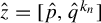
First, we will show that for
$k_n$
 sufficiently large, statements of (2) and (3) hold for
$\hat y = \hat q^{k_n}$
 and
$\hat z = [\hat p, \hat q^{k_n} ]$
 exactly. In order to do this, we use the hyperbolicity of
$\hat q$
 and Lemma 4.2. Then to conclude the proof we will later use continuity to show that (2) and (3) hold for any
$\hat y \in \hat {\sigma }^{-k_n}(R_\rho (\hat q))$
 .
Applying Lemma 4.2 with
$\theta = \min \{\theta _0, \epsilon /2\}$
 and
$\gamma /2$
 for the Lipschitz constant as in the statement of the lemma, we may obtain a constant K such that the conclusion of that lemma holds if
$\sigma _k(A)>K\sigma _{k+1}(A)$
 for a linear map
$A\in \mathrm {SL}(d,\mathbb R)$
 . Since
$\hat q$
 is generic for
$\hat {\mu }$
 and
$\unicode{x3bb} _k(\hat {\mu })> \unicode{x3bb} _{k+1} (\hat {\mu })$
 , for the K specified above if we choose
$k_n$
 large enough, then
$\sigma _k(A^{k_n}(\hat {q}^{k_n}))>K\sigma _{k+1}(A^{k_n}(\hat {q}^{k_n}))$
 . Hence, for any subspace U with
$\angle (U,S_{d-k}(\hat {q}^{k_n}, k_n))> \theta _0$
 , we have that

and
$A^{k_n}$
 is
$\gamma /2$
 -Lipschitz on the same set of U.
Since
$\hat q^{k_n} \in G_l$
 , by (2
$^\prime $
 ) in Claim 4.4 we have
$\angle (E^u( [ \hat p,\hat q^k_n]), E^s(\hat q^{k_n}))> 2 \theta _0$
 . Thus, since
$S_{d-k}(\hat {q}^{k_n},k_n)$
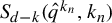 converges to
$E^s(\hat {q}^{n_k})$
 by (4
$^\prime $
 ) in Claim 4.4, for
$k_n$
 sufficiently large we see that we may take
$U = E^u( [ \hat p,\hat q^{k_n}])$
 in (12) to obtain that
$A^{k_n}(\hat q^{k_n})$
 is
$\gamma /2$
 -Lipschitz on a
$\theta _0$
 -neighborhood of
$E^u(\hat z)$
 , verifying (3) for
$\hat y = \hat q^{k_n}$
 . Moreover, since
$U_k(\hat {q}^{k_n}, k_n)$
 converges to
$E^u(\hat q)$
 , (12) with
$U = E^u(\hat z)$
 gives

for n sufficiently large. Thus, we have verified that (2) and (3) hold at exactly
$\hat y = \hat q^{-k_n}$
 as long as
$k_n$
 is sufficiently large, and we now let
$k := k_n$
 for any such large
$k_n$
 .
Finally, we verify that the statements of (2) and (3) hold for all
$\hat y \in \sigma ^{-k}(R_\rho (\hat q))$
 if
$\rho $
 is taken sufficiently large. The key observation is that
$E^u(\hat z)$
 , where
$\hat z = [ \hat p,\hat y]$
 , varies continuously on
$\hat y$
 . Since the cocycle for a fixed k also varies continuously, this implies that (2) and (3) are open conditions on
$\hat y$
 . Since (2) and (3) hold at
$\hat q^{k}$
 , increasing
$\rho $
 if necessary the same holds in the neighborhood
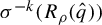
$\sigma ^{-k}(R_\rho (\hat {q}))$
 of
$\hat q^{k}$
 , with
$\epsilon $
 in equation (12) and
$\gamma $
 -Lipschitzness as required for (3).
Now we use the above lemma to construct a set of rectangles such that, given a fixed hyperplane section, there exists some rectangle in the set along which the cocycle can map the unstable direction of a point in the rectangle to avoid the given hyperplane section.
Proposition 4.5. Fix
$\gamma>0$
 and
$\theta _0$
 any sufficiently small number. Then for every
$l \in {\mathbb N}$
 there exist
$N\in {\mathbb N}$
 ,
$\hat q\in \hat {\Sigma }$
 ,
$\rho \in {\mathbb N}$
 , and a finite collection of points
$\{\hat q_i\}_{1\le i \leq N} \subseteq W^s_{\mathrm {loc}}(\hat q)$
 and associated times
$k_i \in {\mathbb N}$
 such that the following assertions hold.
-
(a) $R_\rho (\hat q_i) \cap R_\rho (\hat q_j) = \varnothing $
, for
$i \neq j$
; -
(b) $\hat {\sigma }^{-k_i}(R_\rho (\hat q_i))\subseteq C^u_l(\hat p)$
, for each
$1 \leq i \leq N$
; -
(c) for any hyperplane section H of $\mathrm {Gr}(k,d)$
, there exists some
$i \in \{1,\ldots , N\}$
such that for any Oseledec regular
$\hat y \in \hat {\sigma }^{-k_i}(R_\rho (\hat q_i))$
we have (13) $$ \begin{align} d_{\mathrm{Gr}(k,d)}(A^{k_i}(\hat y)E^u(\hat z), H)> \theta_0, \end{align} $$where $\hat z = [\hat p, \hat y]$
;
-
(d) for $\hat y$
and
$\hat z$
as above,
$A^{k_i}(\hat y)\colon \mathrm {Gr}(k,d)\to \mathrm {Gr}(k,d)$
is
$\gamma $
-Lipschitz on a
$\theta _0$
-neighborhood of
$E^u(\hat z)$





Proof. Let
$\hat {q}$
 be a point such that
$\hat {\mu }^s_{\hat q}$
 -a.e. point in
$W^s_{\mathrm {loc}}(\hat {q})$
 is Oseledec regular and generic for
$\hat {\mu }$
 . We will need the following claim, which we will prove immediately after this proposition for the sake of clarity.
Claim 4.6. For any
$\theta _0> 0$
 sufficiently small, given any hyperplane section
${H\subseteq \mathrm {Gr}(k,d)}$
 , there exists a subset
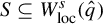
$S \subseteq W^s_{\mathrm {loc}}(\hat q)$
 of positive
$\mu ^s_{\hat q}$
 -measure such that for every
$\hat z \in S$
 ,

Now let
$\theta _0$
 be any sufficiently small number such that Claim 4.6 and Lemma 4.3 hold. Observe that
$\ell$
 is independent of this small
$\theta_0$
 .
Fix a collection of hyperplane sections

with the property that, given any other hyperplane section H, there exists some
$1 \leq i \leq N$
 such that the Hausdorff distance in
$\mathrm {Gr}(k,d)$
 between H and
$H_i$
 is less than
$\theta _0/2$
 . This is possible since the space of hyperplane sections is compact with the Hausdorff distance.
For each
$1 \leq i \leq N$
 , we apply Claim 4.6 with
$H = H_i$
 to obtain a positive
$\mu ^s_{\hat q}$
 -measure set
$S_i \subseteq W^s_{\mathrm {loc}}(\hat q)$
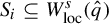 of points
$\hat z$
 with

For each
$1 \leq i \leq N$
 , we let
$\hat q_i$
 be any such point in
$S_i$
 which is, moreover, generic for and Oseledec regular for
$\hat {\mu }$
 . Let
$0<\epsilon <\theta _0$
 and apply Lemma 4.3 with this choice of
$\epsilon ,\theta _0$
 for each
$\hat q_i$
 to obtain a sequence of rectangles
$R_{\rho _i}(\hat {q}_i)$
 satisfying the conclusions of that lemma. Let
$\rho $
 be greater than the maximum of the
$\rho _i$
 and chosen large enough that
$R_\rho (\hat q_i) \cap R_\rho (\hat q_j) = \varnothing $
 , for
$i \neq j$
 , verifying (a). It is evident since the rectangles
$R_\rho (\hat q_i)$
 satisfy the conclusions of Lemma 4.3 that (b) and (d) also hold for the constructed rectangles. It remains to verify (c).
Let H be any hyperplane section of
$\mathrm {Gr}(k,d)$
 . By construction, there is some
$1 \leq i \leq N$
 such that the Hausdorff distance in
$\mathrm {Gr}(k,d)$
 between H and
$H_i$
 is less than
$\theta _0/2$
 . This, together with the fact that
$\angle (E^u(\hat {q}_i),H_i)>2\theta _0$
 , and

by (2) in Lemma 4.3 then gives (c) by the triangle inequality.
We now prove Claim 4.6.
Proof of Claim 4.6.
Let
$\hat {m}$
 be a u-state over
$\hat {\mu }$
 on
$\hat {\Sigma } \times \mathrm {Gr}(k,d)$
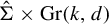 . For a hyperplane section H, let
$H_\theta $
 be its
$\theta $
 -closed neighborhood in
$\mathrm {Gr}(k,d)$
 . Since, by Proposition 3.3,
$m_x(H) = 0$
 for any hyperplane section H, by upper semi-continuity for each
$1 \leq i \leq N$
 there is some
$\theta _i> 0$
 sufficiently small to ensure that
$m_{q}(H_{\theta _i}) < 1/2$
 . By taking
$\theta _0 = \min _{1 \leq i\leq N} \theta _i/3$
 , we see that

Choose a set
$\{H^i\}_{1 \leq i \leq N}$
 of hyperplane sections of
$\mathrm {Gr}(k,d)$
 with the property that any other hyperplane section
$H \subseteq H^i_{\theta _0/2}$
 for some
$1 \leq i \leq N$
 . This is possible since, in the Hausdorff topology, the space of hyperplane sections is compact and the set of hyperplane sections contained in a neighborhood of a fixed hyperplane section contains an open set.
By the disintegration formula,

recalling that, by Proposition 3.5 for
$\hat {\mu }^s_{\hat p}$
 -a.e.
$\hat {x}$
 in
$W^s_{\mathrm {loc}}(\hat q)$
 , we have
$\hat {m}_{\hat {x}} = \delta _{E^u(\hat {x})}$
 .
Now, given an arbitrary hyperplane section H, by construction there is some
${1 \leq i \leq N}$
 such that
$H \subseteq H^i_{\theta _0/2}$
 . Then by equation (14) and the disintegration formula (15), we see that set S of
$\hat {x} \in W^s_{\mathrm {loc}}(\hat q)$
 , with
$E^u(\hat {x}) \notin H^i_{3\theta _0}$
 , must have
$\mu ^s_{\hat q}$
 -measure at least
$1/2$
 . Finally, since
$H \subseteq H^i_{\theta _0/2}$
 , we conclude that for
$\hat {x} \in S$
 , we have
$d_{\mathrm {Gr}}(E^u(\hat {x}), H)> 2\theta _0$
 , as desired.
Remark 4.7. Observe that
$\theta _0$
 does not depend on l in the construction in Proposition 4.5. All other parameters, namely,
$\hat q'$
 ,
$\hat q_i'$
 ,
$k_i$
 ,
$\rho $
 and N, depend on l, but this dependence will not be relevant and we will often omit it.
With the twisting construction done, we now move to the proof of convergence to a Dirac mass. The main idea is to construct, for
$\hat {\mu }$
 -a.e.
$\hat {x}$
 , a suitable subsequence of negative times along which the orbit of
$\hat {x}$
 has some good properties which we now define.
From now on, fix some
$\theta _0$
 sufficiently small so that Proposition 4.5 holds and some
$0 < \gamma < 1$
 . For each
$l> 0$
 , we obtain a set of rectangles
$R_\rho (\hat q_i)$
 as in Proposition 4.5 for the parameters
$\theta _0$
 , l and
$\gamma $
 , which for simplicity we will denote simply by
$R_1^l, \cdots R_N^l$
 .
For each
$\hat {x} \in \hat {\Sigma }$
 and
$n \in {\mathbb N}$
 , let
$k \leq j \leq d-1$
 be the smallest integer such that
$\sigma _j(A^n(\hat {x}^n))> \sigma _{j+1}(A^n(\hat {x}^n))$
 . Then
$S_{d-j}(\hat {x}^n,n)$
 is a well-defined
$(d-j)$
 -dimensional linear subspace which defines some linear section S on
$\mathrm {Gr}(k, d)$
 . Fix
$H_{\hat {x}^n}$
 to be any hyperplane section containing S. If j does not exist, that is,
$\sigma _j(A^n(\hat {x}^n)) = \sigma _{j+1}(A^n(\hat {x}^n))$
 for all
$k \leq j \leq (d-1)$
 , we fix
$H_{\hat {x}^n}$
 to be any hyperplane section of
$\mathrm {Gr}(k, d)$
 .
Definition 4.8. We say that a point
$\hat {x} \in \hat {\Sigma }$
 is l-good if there exists a time
$n_l> l$
 such that the following assertions hold:
-
(1) $\hat {x}^{n_l} \in R_i^l$
for some
$1 \leq i \leq N$
; -
(2) the conclusion of Proposition 4.5(c) with $H = H_{\hat {x}^{n_l}}$
holds for the
$R_i^l$
specified in (1); that is, for any Oseledec regular
$\hat y \in \hat {\sigma }^{-k_i}(R^l_i)$
, we have $$ \begin{align*} d_{\mathrm{Gr}(k,d)}(A^{k_i}(\hat y)E^u(\hat z), H_{\hat{x}^{n_l}})> \theta_0, \end{align*} $$where $\hat z = [\hat p,\hat y]$
.


Proposition 4.9. For each
$l>0$
 and any fully supported shift-invariant probability measure
$\hat \eta $
 on
$\hat {\Sigma }$
 with continuous local product structure, the set of l-good points has full measure with respect to
$\hat \eta $
 .
Before proceeding to the proof we state a lemma. This lemma is an analog of the Lebesgue density theorem for measures with local product structure. It is likely possible to deduce it from Federer’s book [Reference FedererFed69, §2.9], but we expect that this would take longer than reading the proof below.
Lemma 4.10. Let
$\hat \nu $
 be a probability measure with local product structure on
$\hat {\Sigma }$
 and
${0<\alpha <1}$
 . Let
$G\subseteq \hat {\Sigma }$
 be some Borel measurable set. Suppose that for
$\hat \nu $
 -a.e.
$\hat {x}\in \hat {\Sigma }$
 , for
$\hat \nu ^s_{\hat {x}}$
 a.e.
$\hat y\in W^s_{\mathrm {loc}}(\hat {x})$
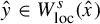 , and for any
$\epsilon>0$
 there exist a set
$S\subset W^s_{\mathrm {loc}}(\hat {x})\cap G$
 and
$0<\epsilon '\le \epsilon $
 , with:
-
(1) $S\subseteq B_{\epsilon '}(\hat {y})$
; -
(2)
$$ \begin{align*}\frac{\hat \nu^s_{\hat{x}}(S)}{\hat \nu^s_{\hat{x}}(B_{\epsilon'}(\hat{y})\cap W^s_{\mathrm{loc}}(\hat{x}))}>\alpha>0;\end{align*} $$
-
(3) $S\cap G$
clopen in
$W^s_{\mathrm {loc}}(\hat {x})$
.


Then
$\hat {\nu }(G)=1$
 .
Proof. Clearly from local product structure it suffices to verify that
$\hat {\nu }^s_{\hat {x}}(G\cap W^s_{\mathrm {loc}}(\hat {x}))=1$
 for
$\hat {\eta }$
 -a.e.
$\hat {x}$
 . We will embed
$W^s_{\mathrm {loc}}$
 into Euclidean space and then make use of the following claim.
Claim 4.11. For each
$m\in {\mathbb N}$
 , there exists
$C_m>0$
 such that if
$\mathbb {P}$
 is a probability measure in
$\mathbb R^m$
 with compact support S and
$G\subseteq S$
 is a set such that for
$\mathbb {P}$
 -a.e.
$x\in S$
 there exist arbitrarily small open balls
$O(x)$
 such that

then
$\mu (G)\ge \alpha /C_m$
 . In fact, if each
$G\cap O(x)$
 contains a closed subset K that is clopen in S such that

then G contains a closed subset of measure at least
$\alpha /C_m$
 that is clopen in S.
Proof. Let
$S'$
 be the subset of full
$\mathbb {P}$
 -measure for which the density property holds. Let
$\mathcal { O } = \{O(x)\}_{x \in S'}$
 be the open cover of
$S'$
 by the sets
$O(x)$
 guaranteed by the condition. Then the Besicovitch covering lemma implies there is some
$C_m$
 such that we may find
$C_m$
 families
$\mathcal { A }_1,\ldots ,\mathcal { A }_{C_m}\subseteq \mathcal { O }$
 such that for each
$1 \leq i\leq C_m$
 the elements of
$\mathcal { A }_i$
 are disjoint and
$S'$
 is contained in the union of all the
$\mathcal { A }_i$
 ’s elements. Letting
$A_i$
 be the union of the sets in
$\mathcal { A }_i$
 , we see that
$\mathbb {P}(A_i\cap G)\ge \alpha \mathbb {P}(A_i)$
 . Hence, as
$\{A_i\}$
 is an at most
$C_m$
 -fold cover of
$S'$
 , which has
$\mathbb {P}(S') = 1$
 , it follows that
$\mathbb {P}(G)\ge \alpha /C_n$
 .
The claim about a closed subset of G follows by taking the clopen in S subsets
$K_i$
 in each
$A_i$
 .
The set
$W^s_{\mathrm {loc}}(\hat {x})$
 is a Cantor set which we may embed Hölder continuously in
$\{0,1\}^{{\mathbb N}}$
 by coding the symbols used to define
$\Sigma $
 . The Cantor set
$\{0,1\}^{{\mathbb N}}$
 has a Hölder continuous embedding in
$\mathbb R$
 as the middle thirds Cantor set by sending each string to the appropriate real number with no
$1$
 s in its ternary expansion. In fact, the embedding into
$\mathbb R$
 carries balls in
$\{0,1\}^{{\mathbb N}}$
 into balls in
$\mathbb R$
 because the embedding is increasing in the obvious way. Let
$\phi $
 denote this particular embedding
$\phi \colon W^s_{\mathrm {loc}}(\hat {x})\to \mathbb R$
 .
Let
$\mathbb {P} = \phi _* \hat \nu ^s_{\hat {x}}$
 denote the pushforward of the measure
$\hat {\nu }^s_{\hat {x}}$
 on Euclidean space under the embedding
$\phi $
 and
$G_\phi = \phi (G) \subseteq \Omega =\phi (W^s_{\mathrm {loc}}(\hat {x}))$
 denote the pushforward of the set of good points. This set is still Borel because it is a Borel subset of a closed subspace. Moreover, as the embedding carries balls in the Cantor set into intervals in the real line, we may apply Claim 4.11, which requires a covering by balls. Thus, we see that there is a closed subset
$K_1\subset G$
 with
$\mathbb {P}(K_1)\ge \alpha /C_1$
 that is clopen in
$\Omega $
 . As
$K_1$
 is clopen in
$\Omega $
 ,
$\Omega _2=\Omega \setminus K_1$
 is a closed set and a positive distance away from
$K_1$
 . Thus,
$\Omega _2$
 also has a covering by balls as in Claim 4.11. And, importantly, because
$\Omega _2$
 is a positive distance from
$K_1$
 , and the balls in Claim 4.11 are arbitrarily small, from Claim 4.11 we obtain another clopen subset
$K_2\subseteq \Omega _2$
 disjoint from
$K_1$
 with measure

We may then consider the set
$\Omega _2\setminus K_2$
 and continue inductively. The
$\mathbb {P}$
 -measure of the complement of
$\sqcup _{i=1}^n K_i$
 goes to zero exponentially quickly and the claim follows.
We now return to the proof that l-good points have full measure.
Proof of Proposition 4.9.
Let
$X_{l}$
 denote the set of l-good points, and let
$R_1,\ldots , R_N$
 be the rectangles guaranteed by Proposition 4.5 applied for the fixed
$\theta _0>0$
 and our choice of
$l\in {\mathbb N}$
 . We proceed by checking the criterion in Lemma 4.10 for
$G=X_l$
 . The point of the proof is that if a point
$\hat {x}$
 visits
$R_i$
 at some point
$\hat {x}^n$
 in its past, then there is some j such that the points in
$W^s_{\mathrm {loc}}(\hat {x}^n)$
 in
$R_j$
 are
$\ell $
 -good. This is because
$A^n(\hat {x}^n)$
 is constant on
$W^s_{\mathrm {loc}}(\hat {x}^n)$
 and this specific linear map is always l-good for the points in some
$R_j$
 .
Let
$R=\sqcup _{1\le i\le N} R_i$
 . The following statement is immediate from the continuous product structure. There exists
$K>1$
 such that for any
$\hat {x}\in R$
 and
$1\le i\le N$
 ,

For
$\hat {\eta }$
 -a.e.
$\hat {x}\in \hat {\Sigma }$
 , there exist infinitely many
$n\ge l$
 such that
$\hat {\sigma }^{-n}(\hat {x})\in R$
 . Consider now the matrix
$A^n(\sigma ^{-n}(\hat {x}))$
 . Note that as the cocycle is constant on local stable leaves, for any
$\hat {x}'\in W^s_{\mathrm {loc}}(\hat {\sigma }^{-n}(\hat {x}))$
 we have that
$A^n(\hat {x}')=A^n(\hat {\sigma }^{-n}(\hat {x}))$
 . By Proposition 4.5, there exists some
$i\in \{1,\ldots , N\}$
 such that if we take
$H=S_{d-d^u}(A^n(\hat {\sigma }^{-n}(\hat {x})))$
 , and any
$\hat {y}$
 in
$R_i\cap W^s_{\mathrm {loc}}(\hat {x}')$
 , then (13) holds for that
$\hat {y}$
 . This means that
$\hat {\sigma }^n(\hat {y})$
 is
$\ell $
 -good at time n.
In particular, we see that all points in
$\hat {\sigma }^n(R_i\cap W^s_{\mathrm {loc}}(\hat {\sigma }^{-n}(\hat {x})))$
 are in
$X_l$
 . Call this set
$G_{n,\hat {x}}$
 . In order to conclude, it suffices to show that there exists some
$D>0$
 independent of
$\hat {x}$
 such that

But by equation (16), this is immediate from Lemma 2.6. We are now done because we verified the criterion in Lemma 4.10.
Finally, we show that the conditional measures for a u-state of
$\hat \eta $
 must also be Dirac masses, that is, Proposition 4.1. The proof will use the following lemma.
Lemma 4.12. Let
$\varepsilon> 0$
 and
$\theta _0> 0$
 . Then there exists
$\delta> 0$
 such that for any
$A \in \mathrm {GL}(d,\mathbb R)$
 the following assertion holds. Fix
$1 \leq k \leq d$
 and suppose that
$q \geq k$
 is the smallest integer such that
$\sigma _q(A)> \sigma _{q+1}(A).$
 Let H be any geometric hyperplane section of
$\mathrm {Gr}(k, d)$
 containing the linear section defined by
$S_q(A)$
 in
$\mathrm {Gr}(k,d)$
 , and if q does not exist (that is,
$\sigma _q(A) = \sigma _{q+1}(A)$
 for
$k \leq q \leq d-1$
 ), let H be any hyperplane section.
Then for any
$\xi _1, \xi _2 \in \mathrm {Gr}(k, d)$
 such that
$d_{\mathrm {Gr}(k,d)}(\xi _i, H)> \theta _0$
 ,
$i = 1,2$
 ,

Proof. Let
$A \in \mathrm {GL}(d,\mathbb R)$
 . Since the metric on the Grassmannian is invariant by isometries of
$\mathbb R^d$
 , by the singular value decomposition theorem we may assume that A is of the form
$A = \text {diag}(a_1, \ldots , a_d)$
 , with
$a_1 \geq \cdots \geq a_d> 0$
 . Without loss of generality we may also assume that H is the hyperplane section defined by
$e_{k+1} \wedge \cdots \wedge e_d$
 .
Thus, we can describe elements of
$\{\xi \in \mathrm {Gr}(k,d): d_{\mathrm {Gr}(k,d)}(\xi , H)> \theta _0\}$
 as graphs with bounded slopes over the first k coordinates, that is, we may embed the preceding set into the set
$\text {End}_M(\mathbb R^k, \mathbb R^{d-k})$
 of linear maps from the first k coordinates to the last
$d-k$
 coordinates of
$\mathbb R^d$
 with a norm bounded by
$M> 0$
 , where M only depends on
$\theta _0$
 . Moreover, it is not hard to see that in this set
$d_{\mathrm {Gr}(k,d)}$
 is equivalent to the distance induced by the operator norm on
$\text {End}_M(\mathbb R^k, \mathbb R^{d-k})$
 . Since all matrix norms are equivalent we endow
$\text {End}_M(\mathbb R^k, \mathbb R^{d-k})$
 with the max norm, that is, for
$\phi \in \text {End}_M(\mathbb R^k, \mathbb R^{d-k})$
 given in a basis by
$\phi _{ij}$
 , we let
$\|\phi \| = \max _{i,j} |\phi _{ij}|$
 .
Let
$\phi _1, \phi _2 \in \text {End}_M(\mathbb R^k, \mathbb R^{d-k})$
 correspond to
$\xi _1, \xi _2 \in \mathrm {Gr}(k,d)$
 as in the hypotheses of the theorem and
$A\phi _1, A\phi _2 \in \text {End}_M(\mathbb R^k, \mathbb R^{d-k})$
 correspond to
$A\xi _1, A\xi _2 \in \mathrm {Gr}(k,d)$
 . To conclude, it suffices to find a uniform bound for
$|(A\phi _1-A\phi _2)_{ij}|$
 in terms of
$|(\phi _1-\phi _2)_{ij}|$
 . It is clear that for any
$\phi \in \text {End}_M(\mathbb R^k, \mathbb R^{d-k})$
 , we have
$|(A\phi )_{ij}| \leq (a_{k+1}/a_k) \dot |\phi _{ij}|$
 , since the action of A expands the first k coordinates by at least
$a_k$
 and the last
$d-k$
 by at most
$a_{k+1}$
 . Since
$a_{k+1}/a_k \leq 1$
 the proof is complete.
Remark 4.13. Observe that the crucial fact is that
$\delta $
 works for any
$A \in \mathrm {GL}(d,\mathbb R).$
 In other words, the action of linear maps in a region uniformly bounded away from the least expanded subspaces is equicontinuous.
Proof of Proposition 4.1.
Since the countable intersection of full measure sets has full measure, by Proposition 4.9, we see that
$\hat \eta $
 -a.e.
$\hat {x}$
 is l-good for every l. Recall that for
$\hat \eta $
 -a.e.
$\hat {x}$
 by Proposition 2.13,

Hence, there is a full
$\hat \eta $
 -measure set
$S \subseteq \hat {\Sigma }$
 such that the above holds and every point in S is l-good for every
$l> 0$
 . Fix any such
$\hat {x}$
 in S. For all
$l> 0$
 fix
$n_l> l$
 to be a time guaranteed by the definition of l-good for
$\hat {x}$
 . We say that a probability measure m on a metric space is
$\varepsilon $
 -concentrated at a point z if
$m(B_{\epsilon }(z))\ge 1-\varepsilon $
 , where
$B_{\epsilon }(z)$
 is the open ball of radius
$\epsilon $
 about z.
Claim 4.14. Let
$\varepsilon> 0$
 . Then for all
$l> 0$
 sufficiently large there is an
$i \in \{1, \ldots ,N\}$
 such that for
$k_i = k_i(l)$
 as in Proposition 4.5, the measure

is
$\varepsilon $
 -concentrated.
We will now show how to conclude given the claim. Since
$n_l> l$
 , by passing to a subsequence of
$n_l$
 we may assume that
$n_{l+1}> n_l+k_i(l)+l$
 , where
$k_i(l)$
 is as in the claim, and that the point around which the masses
$\varepsilon $
 -concentrate converges to some
$\xi ^u(\hat {x}) \in \mathrm {Gr}(k, d)$
 , by compactness of the Grassmannian, from which we conclude that

and the proof is complete. Hence, we are done once we prove the claim about
$\varepsilon $
 -concentration of masses.
Proof of Claim 4.14.
We begin my fixing some constants. Fix some small
$\varepsilon>0$
 . From Proposition 4.5, there exists a fixed
$\theta _0>0$
 such that the conclusions of that proposition hold. For each l, we let
$R_i^{l}$
 denote the collection of rectangles obtained from Proposition 4.5 applied with that fixed choice of
$\theta _0>0$
 . By definition of
$n_l$
 ,
$\hat {x}^{n_l} \in R_i^l$
 for some
$1 \leq i \leq N$
 and a rectangle obtained from Proposition 4.5. Hence,
$\hat {x}^{n_l + k_i} \in C^u_l(\hat p)$
 , where
$k_i$
 is also given by Proposition 4.5.
By Lemma 4.12, given this choice of
$\varepsilon>0$
 and
$\theta _0>0$
 , there exists some
$\delta _1>0$
 such that if m is a measure on
$\mathrm {Gr}(k,d)$
 ,
$A\in \mathrm {GL}(d,\mathbb R)$
 , and m is
$\delta _1$
 concentrated at a point
$V\in \mathrm {Gr}(k,d)$
 that is
$\theta _0$
 away from H, a geometric hyperplane defined by a subspace containing the most contracting subspace
$S_q(A)$
 of A as defined in Lemma 4.12, then
$A_*m$
 is
$\varepsilon $
 -concentrated. Note that this
$\delta _1$
 is not literally the
$\delta $
 from that lemma but may be smaller to ensure that the conclusion of the lemma applies to the set where m is concentrated.
Let
$\alpha =\min \{\theta _0/2,\delta _1\}>0$
 .
We will show
$\varepsilon $
 -concentration by breaking down

into

and pushing the measure through each of these terms in order. We give each of these terms names:


The proof then breaks down into a sequence of three claims, which follow from our choice of constants at the beginning of the proof.
Subclaim 1. The measure
$m_1$
 is
$\alpha $
 -concentrated around
$E^u(\hat z)$
 , where
$\hat z=W^s_{\mathrm {loc}}(\hat {x}^{n_l+k_i})\cap W^u_{\mathrm {loc}}(\hat p)$
 .
Proof. By definition
$\hat {z}\in W^s_{\mathrm {loc}}(\hat {x}^{n_l+k_i})$
 . But note that as
$n_l$
 is an l-good time,
$\hat {x}^{n_l+k_i}\in C^u_l(\hat p)$
 . This implies that
$\hat {x}^{n_l+k_i+l}$
 and
$\hat {z}^l$
 lie in the same local stable leaf. Thus, as the cocycle is constant along local stable leaves,

hence it suffices to show that the right-hand side of (20) is
$\alpha $
 -concentrated around
$E^u(\hat {z})$
 . To see this, note that that

The expression in parentheses converges to
$H^u_{\hat p \hat z}$
 as
$l \to \infty $
 . Moreover,
$A^{l}(\hat p)_* m^{\eta }_{ P(\hat z^{ l})}$
 converges to
$\delta _{E^u(\hat p)}$
 since
$m^{\eta }_{ P(\hat z^{l})}$
 converges weak* to
$m^{\eta }_{\hat p}$
 and the latter gives 0 measure to hyperplane sections. Hence, by Lemma 2.10, we see that the right-hand side of (20) converges to
$\delta _{H^u_{\hat p\hat z}E^u(\hat p)}$
 .
Therefore, for l sufficiently large it follows that

is
$\alpha $
 -concentrated around
$H^u_{\hat p \hat z} E^u(\hat p) = E^u(\hat z)$
 (Lemma 2.3), as desired.
Subclaim 2. The measure
$m_2$
 is
$\delta _1$
 -concentrated at a point at least
$\theta _0$
 away from
$H=H_{\hat {x}^{n_l}}$
 , where H is defined as in the definition of
$\ell $
 -good.
Proof. From Subclaim 1,
$m_1$
 is
$\alpha $
 -concentrated at
$E^u(\hat z)$
 . The application of Proposition 4.4 gives that

and that
$A^{k_i}(\hat {x}^{n_l+k_i})$
 is
$1$
 -Lipschitz in a
$\theta _0$
 -neighborhood of
$E^u(\hat z)$
 . Thus, as
$\alpha <\theta _0$
 , by the
$1$
 -Lipschitzness
$m_2$
 is
$\alpha $
 -concentrated at a point
$\theta _0$
 away from H. As
$\alpha \le \delta _1$
 we are done.
Subclaim 3. The measure
$m_3$
 is
$\varepsilon $
 -concentrated.
Proof. From the conclusion of Subclaim 2, H is a geometric hyperplane defined by a subspace containing the appropriate most contracting subspace of
$A^{n_l}(\hat {x}^{n_l})$
 specified by Lemma 4.12. Thus, by the choice of
$\delta_1$
 in the second paragraph of the proof of Claim 4.14, as
$m_2$
 is
$\delta _1$
 -concentrated
$\theta _0$
 away from H, it follows that
$m_3$
 is
$\varepsilon $
 -concentrated.
We are now done with the proof of Claim 4.14 as Subclaim 3 is the conclusion needed.
Having finished the proof of Claim 4.14, we obtain the proof of Proposition 4.1 by the discussion after the statement of that claim.
5 Conclusion of the proof of Theorem B
In Proposition 4.1 from the previous section we obtained a measurable
$\xi ^u\colon \hat {\Sigma } \to \mathrm {Gr}(k, d)$
 defined
$\hat \eta $
 almost everywhere. This section satisfies the same properties as the map
$\xi ^u$
 considered in [Reference Avila and VianaAV07a, Proposition 6.4] where it is shown to have the following properties for
$\hat \eta $
 -a.e.
$\hat {x} \in \hat {\Sigma }$
 :
-
(i) $\xi ^u$
is invariant under the cocycle and the unstable holonomies; -
(ii) $\sigma _{k}(\hat {A}^n(\hat {\sigma }^{-n}(\hat {x})))/\sigma _{k+1}(\hat {A}^n(\hat {\sigma }^{-n}(\hat {x}))) \to \infty $
, and the image of the k-dimensional subspace most expanded by
$\hat {A}^n(\hat {\sigma }^{-n}(\hat {x}))$
converges to
$\xi ^u(\hat {x})$
.


The idea of the rest of the proof of Theorem B is to show that the section
$\xi ^u$
 is the sum of the k strictly largest Oseledec subbundles for
$\hat {A}$
 with respect to
$\hat \eta $
 . To do so, we first obtain an
$\hat \eta $
 -almost everywhere defined section
$\xi ^T\colon \hat {\Sigma } \to \mathrm {Gr}(k, d)$
 by the same argument as in the proof of Proposition 4.1, whose orthogonal complement
$\xi ^s$
 is a candidate sum of the
$(d-k)$
 strictly smallest Oseledec subbundles for
$\hat {A}$
 with respect to
$\hat \eta $
 . Finally, we show that indeed the Lyapunov exponents along
$\xi ^u$
 are strictly greater than those of
$\xi ^s$
 .
To obtain
$\xi ^T$
 , we apply Proposition 4.1 to the adjoint cocycle to
$\hat {A}$
 , which is defined by
$\hat {B}(\hat {x}) := \hat {A}(\hat {\sigma }^{-1}(\hat {x}))^T$
 , where the T superscript denotes transpose with respect to a fixed inner product on
$\mathbb R^d$
 . By definition, the adjoint cocycle
$\hat {B}$
 is a cocycle over
$\hat {\sigma }^{-1}$
 . It is easily verified [Reference Avila and VianaAV07a, §7.1] that the adjoint cocycle is also fiber-bunched and satisfies the integrability hypothesis of the Oseledec theorem. From the assumption
$\unicode{x3bb} _{k}(\hat {A}, \hat {\mu })> \unicode{x3bb} _{k+1}(\hat {A}, \hat {\mu })$
 , it is easy to see that
$\unicode{x3bb} _{k}(\hat {B}, \hat {\mu })> \unicode{x3bb} _{k+1}(\hat {B}, \hat {\mu })$
 since
$\hat {A}$
 and
$\hat {B}$
 have the same singular values. Moreover, we have the following claim.
Claim 5.1. For any
$1 \leq k \leq d-1$
 , the cocycle
$\hat {A}$
 is strongly irreducible on
$\mathrm {Gr}(k, d)$
 if and only if the adjoint cocycle
$\hat {B}$
 is strongly irreducible on
$\mathrm {Gr}(d-k, d)$
 .
Proof. By duality it suffices to show one of the directions, so we prove that
$\hat {A}$
 is strongly irreducible on
$\mathrm {Gr}(k, d)$
 if
$\hat {B}$
 is strongly irreducible on
$\mathrm {Gr}(d-k, d)$
 .
Suppose for contradiction that
$\hat {B}$
 is not strongly irreducible on
$\mathrm {Gr}(d-k, d)$
 , that is, that there exists a non-trivial continuous family of
$(d-k)$
 -linear arrangements
$\mathcal {L}$
 invariant by
$\hat {B}$
 . We define
$\mathcal {L}^T$
 to be a continuous family of k-linear arrangements given by
$\mathcal {L}^T = \star \mathcal {L}$
 , where
$\star $
 is the usual Hodge star map
$\Lambda ^{d-k} \mathbb R^d \to \Lambda ^{k} \mathbb R^d$
 restricted to the Grassmannian. Since the Hodge star map is linear, we see that
$\mathcal {L}^T$
 is by definition a continuous family of k-linear arrangements, and since
$\star $
 sends rank 1 vectors to rank 1 vectors
$\mathcal {L}^T$
 must be non-trivial.
Moreover, since restricted to the Grassmannians the Hodge star maps subspaces to their orthogonal complements, and the transpose cocycle has the property that
$\star A\xi = A^T \star \xi $
 for all subspaces
$\xi $
 , we see that
$\mathcal {L}^T$
 must be invariant by
$\hat {A}$
 . This contradicts strong irreducibility of
$\hat {A}$
 on
$\mathrm {Gr}(k, d)$
 .
Therefore we may apply Proposition 4.1 to the cocycle
$\hat {B}$
 and obtain a section
$\xi ^T\colon \hat {\Sigma } \to \mathrm {Gr}(k, d)$
 and let
$\xi ^s\colon \hat {\Sigma } \to \mathrm {Gr}(d-k, d)$
 be obtained by taking the orthogonal complement of
$\xi ^T$
 . The proof of the Lyapunov exponent gaps of
$\xi ^u$
 and
$\xi ^s$
 now follows in the exact same way as the proof of the main theorem in [Reference Avila and VianaAV07a, §7.2]. For the reader’s convenience we include an outline below.
Outline of proof of Theorem B.
The proof is broken down into several steps.
Step 1:
$\xi ^u(\hat {x})$
 and
$\xi ^s(\hat {x})$
 intersect transversely for
$\hat \eta $
 -a.e.
$\hat {x}$
 .
Proof. Recall that for the reduced cocycle the stable holonomies are trivial. Hence, for
$\hat \eta $
 -a.e.
$\hat {x}$
 ,
$\xi ^s$
 is constant on
$W^s_{\mathrm {loc}}(\hat {x})$
 . Fix one such
$\hat {x}$
 and let H be the hyperplane section defined by
$\xi ^s$
 on
$\mathrm {Gr}(k, d)$
 . By Propositions 3.3 and 3.5, the distribution of
$\xi ^u$
 on
$W^s_{\mathrm {loc}}(\hat {x})$
 avoids a fixed hyperplane section
$\hat \eta ^s_{\hat {x}}$
 -almost everywhere. In particular, it avoids H, so that
$\xi ^u$
 and
$\xi ^s$
 intersect transversely
$\hat \eta ^s_{\hat {x}}$
 -almost everywhere on
$W^s_{\mathrm {loc}}(\hat {x})$
 . Since this holds for
$\hat \eta $
 -a.e.
$\hat {x}$
 , the proof is complete.
Thus, we have
$\hat \eta $
 -almost everywhere defined
$\hat {A}$
 invariant transverse sections
$\xi ^u$
 and
$\xi ^s$
 , so each of these bundles has a splitting into subspaces at
$\hat {\eta }$
 -a.e. point. Let
$\xi _1 \subseteq \xi ^u$
 be the bundle corresponding to the weakest Lyapunov subspace in
$\xi ^u$
 and let
$\xi _2 \subseteq \xi ^s$
 be the bundle corresponding to the strongest Lyapunov subspace in
$\xi ^s$
 . Let
$d_1, d_2$
 be the dimensions and
$\unicode{x3bb} _1, \unicode{x3bb} _2$
 be the exponents of
$\xi _1$
 and
$\xi _2$
 . The proof will be completed if we show
$\unicode{x3bb} _1> \unicode{x3bb} _2$
 .
Define, for
$n \geq 0$
 ,

where
$\det (A, V)$
 denotes the determinant of A restricted to V. Then by the Oseledec theorem,

so it suffices to show that
$ \log \Delta ^n(\hat {x})$
 grows linearly.
Step 2: For
$\hat \eta $
 -a.e.
$\hat {x}$
 ,

Proof sketch.
The idea of the proof is to use the defining property of
$\xi ^u$
 which we mentioned at the beginning of the section, namely that

and that the image of the k-dimensional subspace most expanded by
$\hat {A}^n(\hat {\sigma }^{-n}(\hat {x}))$
 converges to
$\xi ^u(\hat {x})$
 . This, combined with the transversality statement of Step 1, suffices to show divergence of the ratio of the determinants in the definition of
$\Delta ^n$
 and obtain equation (21). For details, see [Reference Avila and VianaAV07a, Proposition 7.3].
Step 3: To conclude one uses the following well-known result. Let
$T\colon X \to X$
 be a measurable transformation preserving a probability measure
$\nu $
 in X, and
$\phi \colon X \to \mathbb R$
 be a
$\nu $
 -integrable function such that

at
$\nu $
 -a.e. point. Then
$\int _X \phi \, d\nu> 0$
 .
The proof is then finished by applying the statement above to
$\log \Delta (x)$
 and applying the Birkhoff ergodic theorem.
6 Furstenberg’s theorem
In this section we show an analog of Furstenberg’s theorem in the fiber-bunched setting. Compare the following theorem with [Reference Bonatti, Gómez-Mont and VianaBGMV03, Theorem 1], which offers a similar alternative between every measure being hyperbolic and there existing a holonomy-invariant measure on the projective extension of the cocycle. The measure obtained in that theorem represents the flags obtained in the proof below.
Theorem C. Suppose that
$\hat {\Sigma }$
 is a transitive hyperbolic system and that
$\hat {A}\colon \Sigma \to \mathrm {GL}(d,\mathbb R)$
 is a fiber-bunched Hölder continuous cocycle that is strongly irreducible on
$\mathrm {Gr}(1,d)$
 . Then exactly one of the following assertions holds:
-
(1) for every measure $\hat {\mu }$
with full support and continuous product structure
$\hat {\mu }$
has two distinct Lyapunov exponents; -
(2) $\hat {A}$
preserves a Hölder continuous conformal structure, and thus every invariant measure has all Lyapunov exponents equal to
$0$
.


Proof. Suppose that there exists some other such measure that has only one Lyapunov exponent. Then by [Reference Kalinin and SadovskayaKS13, Theorem 3.4], there exists a finite cover
$\widetilde { \mathcal { E } }$
 of the cocycle on which we have that the cocycle preserves a continuous flag

and continuous invariant conformal structures on each quotient
$\widetilde { \mathcal { E } }^{i+1}/\widetilde { \mathcal { E } }^i$
 . This flag projects down to a collection of invariant subspaces contained in the original bundle
$\mathcal { E }$
 . Hence, strong irreducibility implies that
$\widetilde { \mathcal { E } }^1=\widetilde { \mathcal { E } }^k$
 , so the original cocycle preserves a conformal structure. Hence, all invariant measures on
$\hat {\Sigma }$
 have a single Lyapunov exponent and the result follows.
Note that the above theorem gives no information on whether there are more than two exponents.
Acknowledgements
The authors thank their advisor, Amie Wilkinson, for suggesting that they study Lyapunov exponents together, which lead to the results in this paper. The authors also thank Jairo Bochi and Aaron Brown for helpful discussions and comments on the manuscript. J.D. is supported by the National Science Foundation under award no. DMS-2202967.
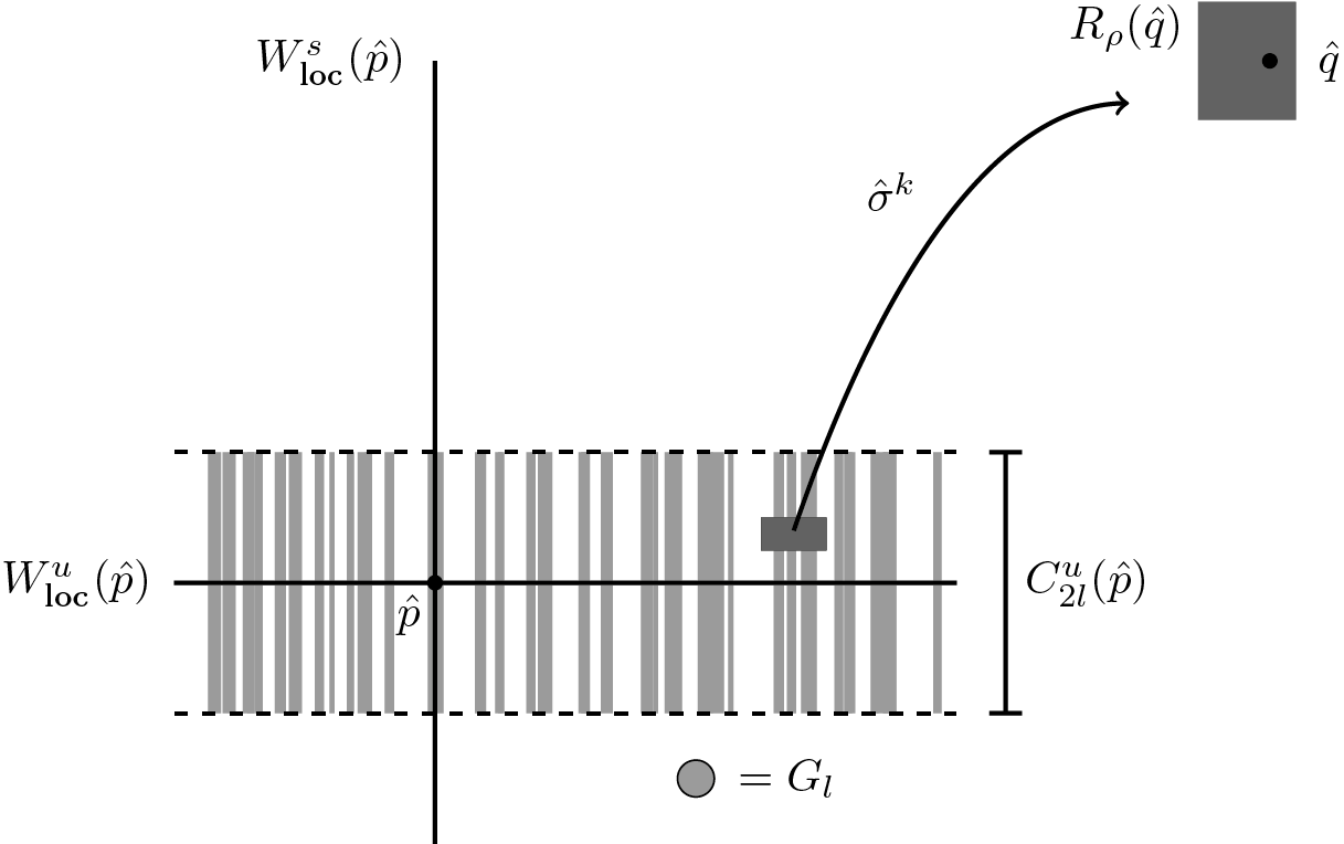


 Open access

