1. Introduction
Safety and dependability is a crucial issue in many industries, which has led to the development of a huge amount of literature devoted to the so-called reliability theory. In the oldest literature the lifetimes of industrial systems or components were usually directly modeled through random variables; see, e.g. [Reference Barlow and Proschan2] for pioneering work on this subject. Based on the development of online monitoring which allows the effective measurement of a system deterioration, numerous papers nowadays model the degradation in itself, which is often considered to be accumulating over time. This is done through the use of continuous-time stochastic processes, which are usually assumed to be monotonous or with a monotonous trend. Most common models include gamma processes [Reference Abdel-Hameed1], [Reference žinlar, Bažant and Osman7], [Reference Van Noortwijk26], Wiener processes with trend [Reference Doksum and Hóyland9], [Reference Whitmore29], and inverse Gaussian processes [Reference Wang and Xu27], [Reference Ye and Chen30] (see also [Reference Kahle, Mercier and Paroissin14] for more references). All these models are (possibly nonhomogeneous) Lévy processes and, hence, have independent increments. However, in an application context, one could think that the current deterioration level of a system can have some influence on its future deterioration development. Typically, when the deterioration rate is increasing over time, one could expect that the more severe a system history is (and, hence, the higher the current deterioration level is), the higher the future deterioration rate. Such behavior cannot be modeled through processes with independent increments and some new ‘state-dependent wear models’ (according to the vocabulary of [Reference Giorgio, Guida and Pulcini11]) need to be developed.
Some interesting attempts have been made in the previous literature for taking into account some stochastic dependence between the current state of a system and its future deterioration, such as [Reference Lemoine and Wenocur17] and [Reference Wenocur28], where the deterioration process is constructed as the solution of a stochastic differential equation (see also [Reference Singpurwalla25]). However, these models do not seem to be very tractable, and up to our knowledge, generic tools still need to be developed for their practical use in an application context (such as estimation procedures). See, however, [Reference Giorgio, Guida and Pulcini11] for a practical use of such models in a specific setting. Another attempt has been made recently by Giorgio, Guida, and Pulcini in a series of papers [Reference Giorgio, Guida and Pulcini12], [Reference Giorgio, Guida and Pulcini13], [Reference Giorgio and Pulcini10], where they suggested considering gamma processes transformed by increasing functions. This provides a tractable Markovian state-dependent wear process. Here we propose using a similar procedure for general Lévy processes, which leads to a more generic state-dependent wear process that we call a transformed Lévy process. The new process includes, for example, transformed gamma processes in the sense of [Reference Giorgio, Guida and Pulcini12], [Reference Giorgio, Guida and Pulcini13], and [Reference Giorgio and Pulcini10], but also classical geometric Brownian motion (see, e.g. [Reference Ross22]). As will be seen, a transformed Lévy process remains a tractable Markov process, for which the Markov kernel is easily obtained. This allows us to derive the joint probability density function of successive observations of a deterioration path, from where a classical maximum likelihood estimation procedure could be easily implemented (which is beyond the scope of the present paper). The model hence has a clear potential for practical use. For a better understanding of its modeling ability, here we focus on stochastic monotonicity/comparison results and on positive dependence properties.
The paper is organized as follows. In Section 2 we define the transformed Lévy process and derive the first distributional properties. Considering a system with deterioration level modeled by a transformed Lévy process, Section 3 is devoted to the study of the impact of the current state of the system on its future deterioration level, from a stochastic monotonicity point of view. We develop positive dependence properties in Section 4 and stochastic monotonicity of increments in Section 5. Concluding remarks are given in Section 6.
2 Definition and the first properties
Throughout the paper, the term Lévy process stands for a possibly nonhomogeneous Lévy process. These processes are also called additive processes in the literature [Reference Sato23, p.3]. We recall that a process
 $${({X_t})_{t \ge 0}}$$
is said to be a (nonhomogeneous) Lévy (or additive) process if
 $$X_{0}=0$$
almost surely (a.s.);
-
$$( X_{t}) _{t \ge 0}$$
has independent increments;
-
$$( X_{t}) _{t \ge 0}$$
is stochastically continuous;
-
$$( X_{t}) _{t \ge 0}$$
has right-continuous paths with left-side limits, almost surely.


We refer the reader to [23, p.3] for more details.
Definition 1. Let
 $$( X_{t}) _{t \ge 0}$$
be a Lévy process with range J, where
 $$J=\mathbb{R}$$
,
 $$J=\mathbb{R}_{+}$$
, or
 $$J=\mathbb{R}_{-}.$$
Let g be a (strictly) increasing differentiable function such that
 $$g\colon
I\subset \mathbb{R}\to J$$
with
 $$g(I)=J$$
. A process
 $$( Z_{t})
_{t \ge 0}$$
is called a transformed (TR) Lévy process with baseline process
 $$( X_{t}) _{t \ge 0}$$
and state function g if
 $$Z_{t}
=g^{-1}( X_{t}) $$
for all
 $$t \ge 0$$
.
We first start with a well-known example.
Example 1. Let
 $$( X_{t}) _{t \ge 0}$$
be a time-scaled Wiener process with drift
 $$X_{t}=A( t) +\sigma~W_{A( t) } \quad\text{for all } t \ge 0,$$
where
 $$( W_{t}) _{t \ge 0}$$
is a standard Wiener process such that
 $${{\rm{W}}_t}\~{\rm{t}}{\mkern 1mu} ({\rm{0}},{\rm{t}})$$]></tex-math>
</alternatives>
</inline-formula> and <inline-formula>
<alternatives>
<inline-graphic xlink:href="S0001867819000211_inline19" mime-subtype="gif" xlink:type="simple"/>
<tex-math>
<![CDATA[$$A\colon \mathbb{R}_{+}
\rightarrow\mathbb{R}_{+}$$
is increasing such that
 $$A( 0) =0$$
and
 $$\lim_{t\rightarrow+\infty}A( t) =+\infty$$
. Such a function is called a time-scaling function in the following. Then
 $$( X_{t}) _{t \ge 0}$$
is a (nonhomogeneous) Lévy process and each increment
 $$X_t-X_s$$
is normally distributed
 $$t\>(A(t) - A(s),{\sigma ^2}(A(t) - A(s)))$$
, where
 $$0\leq s \lt t$$
. Considering
 $$z_{0}>0$$
and
 $$g( x) =\ln( {x}/{z_{0}})
$$
for
 $$x\in\mathbb{R}_{+}^{\ast}$$
, we have
 $$g^{-1}( z)
=z_{0}\mathrm{e}^{z}$$
and
 $$Z_{t}=g^{-1}( X_{t}) =z_{0}\mathrm{e}^{X_{t}}=z_{0}\mathrm{e}^{ A(t) +\sigma~W_{A( t) }} $$
is a time-scaled geometric Brownian motion, and, hence, appears as a specific TR Lévy process.
Note that, if
 $$( X_{t}) _{t \ge 0}$$
is a Lévy process then
 $$({-}X_{t}) _{t \ge 0}$$
is also a Lévy process so that
 $$( g({-}X_{t}) ) _{t \ge 0}$$
with g increasing is a TR Lévy process. Then, any
 $$( \overline{g}( X_{t})
) _{t \ge 0}$$
with
 $$\overline{g}( x) =g({-}x) $$
decreasing is a TR Lévy process in the sense of the previous definition, and, hence, includes the case of any strictly monotonic function g.
In all the following, we assume that
 $$X_{t}$$
admits a probability density function (PDF) with respect to a Lebesgue measure denoted by
 $$f_{X_{t}}$$
. The corresponding cumulative distribution function (CDF) and survival function are denoted by
 $$F_{X_{t}}$$
and
 $$\overline{F}_{X_{t}}$$
, respectively. We use similar notation for other random variables, without further notification.
We now consider the probabilistic structure of a TR Lévy process.
Proposition 1. With the notation of Definition 1, a TR Lévy process is a Markov process with Markov transition kernel provided by
 $$\begin{equation}
P( s,t;\,z,\!\,\mathrm{d} x) =\mathbb{P}( Z_{t}\in \,\mathrm{d} x\ \,\,|\, \ \,
Z_{s}=z) =\,f_{Z_{t}\ \,\,|\, \ \, Z_{s}=z}( x) \,\mathrm{d} x,
\label{eqn1}
\end{equation}
$$
with
 $$\begin{equation}
f_{Z_{t}\ \,\,|\, \ \, Z_{s}=z}( x) =g^{\prime}( x)\, f_{X_{t}
-X_{s}}( g( x) -g( z) )
\label{eqn2}
\end{equation}
$$
and
 $$\begin{equation*}
P( s,t;\,z,( x,\infty) ) =\overline{F}_{Z_{t}\ \,\,|\, \ \,
Z_{s} =z}( x) =\overline{F}_{X_{t}-X_{s}}( g(
x) -g( z) )
\end{equation*}
$$
for all
 $$0\leq s\lt t$$
and all
 $$x,z\in I$$
.
Proof. Based on the fact that the baseline process
 $$( X_{t})
_{t \ge 0}$$
is a Markov process, it is clear that a TR Lévy process
 $$( Z_{t}=g^{-1}( X_{t}) ) _{t \ge 0}$$
is also a Markov process. Also,
 $$\begin{align*}
P( s,t;\,z,( x,\infty) ) & =\mathbb{P}(
Z_{t}>x\ \,\,|\, \ \, Z_{s}=z)
\\
& =\mathbb{P}( X_{t}>g( x) \ \,\,|\, \ \, X_{s}=g( z))
\\
& =\mathbb{P}( X_{t}-X_{s}>g( x) -g( z) \ \,\,|\, \ \,
X_{s}=g( z) )
\\
& =\mathbb{P}( X_{t}-X_{s}>g( x) -g( z))
\\
& =\overline{F}_{X_{t}-X_{s}}( g( x) -g( z)),
\end{align*}
$$
due to the independent increments of
 $$( X_{t}) _{t \ge 0}$$
in the fourth line.
The result for
 $$f_{Z_{t}\ \,\,|\, \ \, Z_{s}=z}( x) $$
is obtained through differentiation of
 $$\mathbb{P}( Z_{t}>x\ \,\,|\, \ \, Z_{s}=z) $$
with respect to x, completing the proof.
>Remark 1. Giorgio et al. [Reference Giorgio, Guida and Pulcini12] considered a transformed gamma process
 $$( Z_{t}) _{t \ge 0},$$
which they define as a Markov process such that the conditional survival function of
 $$Z_{t}-Z_{s}$$
given
 $$Z_{s}=z$$
is of the shape
 $$\overline{F}_{Z_{t}-Z_{s}\ \,\,|\, \ \, Z_{s}=z}( x)
=\overline{F}_{X_{t}-X_{s}}( g( z+x) -g( z))
$$
for all
 $$0\leq s\lt t$$
and all
 $$x,z\geq0$$
, where
 $$\ g\colon \mathbb{R}_{+}
\to \mathbb{R}_{+}$$
and the baseline process
 $$( X_{t})
_{t \ge 0}$$
is a gamma process. This means that their transformed gamma process is defined as a Markov process with Markov transition kernel provided by
 $$( 1) $$
. However, in order to get a consistent definition, it might have been necessary to show, as a preliminary step, that
 $$( 1) $$
actually gives rise to a Markov transition kernel, namely, that
 $$\begin{equation}
\int_{\{ x\in I\} }P( s,t;\,z,\!\,\mathrm{d} x) =1
\label{eqn3}
\end{equation}
$$
and
 $$\begin{equation}
\int_{\{ x\in I\} }P( s,t;\,z,\!\,\mathrm{d} x) P(
t,u;\,x,\!\,\mathrm{d} y) =P( s,u;\,z,\!\,\mathrm{d} y)
\label{eqn4}
\end{equation}
$$
for all
 $$0\leq s \lt t$$
and all
 $$z\in I$$
. In our definition, it is not necessary to verify this step because
 $$ ( 1 ) $$
is obtained by computing the kernel of a Markov process and, consequently,
 $$ ( 3 ) $$
and
 $$ ( 4 )
$$
necessarily hold. As a by-product, this shows the coherency of the definition of a transformed gamma process as proposed in [12]. Also, their definition leads to a similar notion to ours, in the specific context of gamma processes.
We now provide the conditional distribution of an increment of a TR Lévy process given its present state. The proof is a direct consequence of Proposition 1 and it is omitted.
Corollary 1. For all
 $$0\leq s\lt t$$
and
 $$x,z\in I$$
, the conditional survival function of
 $$Z_{t}-Z_{s}$$
given
 $$Z_{s}=z$$
is
 $${\bar F_{{Z_t} - {Z_s}\;{\kern 1pt} {\kern 1pt} |{\kern 1pt} \;{\kern 1pt} {Z_s} = z}}(x) = {\bar F_{{X_t} - {X_s}}}(g(z + x) - g(z)),$$
and the conditional PDF of
 $$Z_{t}-Z_{s}$$
given
 $$Z_{s}=z$$
 $$\begin{equation}
f_{Z_{t}-Z_{s}\ \,\,|\, \ \, Z_{s}=z} ( x ) =g^{\prime} ( x+z )\,
f_{X_{t}-X_{s}} ( g ( x+z ) -g ( z ) ) .
\label{eqn5}
\end{equation}
$$
In a general setting, the increment
 $$Z_{t}-Z_{s}$$
hence depends on its past through
 $$Z_{s}$$
, and the increments of
 $$(Z_{t})_{t \ge 0}$$
are not independent. However, it is easy to characterize the case where the increments are independent, as in the following corollary.
Corollary 2. A TR Lévy process has independent increments if and only if g is of the shape
 $$g ( z ) =az+b$$
, with
 $$a>0$$
and
 $$b\in\mathbb{R}$$
.
Proof. Assume that
 $$g ( z ) =az+b$$
, with
 $$a>0$$
. Then
 $$Z_{t}=g^{-1} ( X_{t} ) = {(X_{t}-b)}/{a}$$
for all
 $$t \ge 0$$
and
 $$ ( Z_{t} ) _{t \ge 0}$$
clearly has independent increments.
Conversely, assume that
 $$ ( Z_{t} ) _{t \ge 0}$$
has independent increments. Then
 $$\overline{F}_{Z_{t}-Z_{s}\ \,\,|\, \ \, Z_{s}=z} ( x ) $$
is independent on z for all
 $$x\in I$$
and all
 $$0\leq s\lt t$$
. Based on Corollary 1, this entails that
 $$g ( z+x ) -g ( z ) $$
is independent on z for all
 $$x\in I$$
, which means that
 $$g^{\prime}$$
is a constant and provides the result.
Considering the fact that a Lévy process is assumed to start from 0 (
 $$Z_{0}=0$$
), the only case for which a TR Lévy process is a Lévy process hence corresponds to a linear function
 $$g ( x ) =ax$$
with
 $$a>0$$
(which entails that
 $$Z_{t}={X_{t}}/{a}$$
for all
 $$t \ge 0$$
).
Corollary 1 allows us to easily write down the joint PDF of increments of a TR Lévy process on successive time intervals as in the following proposition, which could be used for the development of a likelihood estimation procedure in a parametric setting, based on successive observations of deterioration data. See, e.g. [Reference Giorgio, Guida and Pulcini12] and [Reference Giorgio, Guida and Pulcini13] in the specific case of transformed gamma processes.
Proposition 2. Let
 $$0\lt t_{1}\lt \cdots\lt t_{n},$$
and let
 $$Z_{t_{i-1},t_{i}}=
Z_{t_{i}}-Z_{t_{i-1}}$$
for
 $$i\in\{2,\dots,n\}$$
. The PDF of
 $$ (
Z_{t_{1}},Z_{t_{1},t_{2}},\ldots,Z_{t_{n-1},t_{n}} ) $$
is equal to
 $$\begin{align*}
&f_{ ( Z_{t_{1}},Z_{t_{1},t_{2}},\ldots,Z_{t_{n-1},t_{n}} )
} ( z_{1},\ldots,z_{n} )
\\
&\qquad =g^{\prime} ( z_{1} )\, f_{X_{t_{1}} } ( g (
z_{1} )-g(0) ) \prod_{i=1}^{n-1}g^{\prime} ( z_{1:
i+1} )\,f_{X_{t_{i} ,t_{i+1}}} ( g ( z_{1: i+1} )
-g ( z_{1: i} ) ),
\end{align*}
$$
where
 $$z_{1: i}=\smash{\sum_{j=1}^{i}z_{j}}$$
for
 $$1\leq i\leq n$$
.
Proof. Using successive conditioning, we have
 $$\begin{align*}
f_{( Z_{t_{1}},Z_{t_{1},t_{2}},\ldots,Z_{t_{n-1},t_{n}}) } (
z_{1},\ldots,z_{n} ) &=\,f_{Z_{t_{1}}} ( z_{1} )
\prod_{i=1}^{n-1}f_{Z_{t_{i},t_{i+1}}|\bigcap_{j=1}^{i} \{Z_{t_{j-1},t_j}
=z_j\}} ( z_{i+1} )
\\
&=\,f_{Z_{t_{1}}} ( z_{1} )
\prod_{i=1}^{n-1}f_{Z_{t_{i},t_{i+1}}|\bigcap_{j=1}^{i}\{Z_{t_{j}}
=z_{1\colon j}\}} ( z_{i+1} ),
\end{align*}
$$
where, in the first line,
 $$t_0=0$$
. The Markov property now provides
 $$f_{( Z_{t_{1}},Z_{t_{1},t_{2}},\ldots,Z_{t_{n-1},t_{n}}) } (
z_{1},\ldots,z_{n} ) \,=\,f_{Z_{t_{1}}} ( z_{1} )
\prod_{i=1}^{n-1}f_{Z_{t_{i},t_{i+1}}\ \,\,|\, \ \, Z_{t_{i}}=z_{1\colon i}} (
z_{i+1} )
$$
and the result follows from (2) and (5).
We end this section by noting that, given the present state, the future increment process still behaves according to a TR Lévy process. According to the vocabulary of [5], this means that a TR Lévy process possesses the ‘restarting property’.
Proposition 3. (Restarting property)
For a fixed
 $$s>0$$
, set
 $$\smash{Z_{t}^{ ( s ) }}=Z_{t+s}-Z_{s}$$
for all
 $$t \ge 0$$
. Then, given
 $$Z_{s}=x$$
, the process
 $$\smash{( Z_{t}^{ ( s ) })
_{t \ge 0}}$$
is conditionally a TR Lévy process with baseline Lévy process
 $$\smash{X^{ ( s ) }=( X_{t}^{ ( s ) }}=X_{t+s}-X_{s})
_{t\geq 0}$$
and state function
 $$g^{ ( x ) }=g (
x+\cdot ) -g ( x ) $$
.
Proof. We write ‘
 $$\,\stackrel{\text{I.D.}}{=}\, $$
’ for ‘identically distributed as’. Then
 $$\begin{align*}
[ ( Z_{t}^{( s) }) _{t \ge 0}\ \,\,|\, \ \,
Z_{s}=x] & \,\stackrel{\text{I.D.}}{=}\, [ ( Z_{t+s}-Z_{s}) _{t\geq 0}\ \,\,|\, \ \,
Z_{s}=x]
\\
& \,\stackrel{\text{I.D.}}{=}\, [ ( g^{-1} ( X_{t+s} -X_{s}+g ( x )
) -x ) _{t \ge 0}\ \,\,|\, \ \, X_{s}=g ( x ) ]
\\
& \,\stackrel{\text{I.D.}}{=}\, ( g^{-1} ( X_{t+s}-X_{s}+g ( x ) )
-x ) _{t \ge 0}
\end{align*}
$$
based on the independent increments of
 $$(X_{t})_{t \ge 0}$$
for the last line. Hence, given
 $$Z_{s}=x$$
, the process
 $$\smash{( Z_{t}^{ ( s ) })
_{t \ge 0}}$$
conditionally is a TR Lévy process with baseline Lévy process
 $$\smash{X^{ ( s ) }}=(\smash{ X_{t}^{ ( s ) }}=X_{t+s}-X_{s})
_{t \ge 0}$$
and
 $$( g^{ ( x ) }) ^{-1} ( z ) =g^{-1} ( z+g (x) ) -x,$$
or, equivalently,
 $$\smash{g^{ ( x ) } ( y )} =g ( x+y ) -g ( x ) $$
.
Some of the results of the paper require the baseline Lévy process
 $$ ( X_{t} ) _{t \ge 0}$$
to be nonnegative (or at least to keep a constant sign). We recall that this entails that
 $$ ( X_{t} )
_{t \ge 0}$$
is nondecreasing. In that case,
 $$ ( Z_{t} )
_{t \ge 0}$$
is a nondecreasing process with range
 $$[g ( 0 )
,g ( \infty ) )$$
. For ease, we will also assume that
 $$g (
0 ) =0 (\!=Z_{0} ) $$
. This assumption will be referred to as the ‘positive assumption’ in the following. Note that dual results could be written under a similar ‘negative assumption’.
3 Influence of the current state of a TR Lévy process on its future
In this section we investigate the influence of the current state on an increment of the future deterioration process and on its overall cumulated level. We refer the reader to [Reference Müller and Stoyan20] and [Reference Shaked and Shanthikumar24] for the definitions of the stochastic orders used in this section: usual stochastic order, ‘
 $$\prec_{\rm st}$$
’, hazard rate order, ‘
 $$\prec_{\rm hr}$$
’, reverse hazard rate order, ‘
 $$\prec_{\rm rh}$$
’, and likelihood ratio order, ‘
 $$\prec_{\rm lr}$$
’. We refer the reader to [18] for the ageing properties used in this section: increasing hazard rate (IHR), decreasing hazard rate (DHR), decreasing reverse hazard rate (DRHR), and increasing reverse hazard rate (IRHR).
3.1 Influence of the current state on an increment of the wear process
Lemma 1. Let
 $$0\lt s\lt t$$
.
-
$$ [ Z_{t}\ \,\,|\, \ \, Z_{s}=z ] $$
increases in the usual stochastic ordering as z increases.
Assume that g is concave (respectively convex). Then, under the positive assumption,
$$[ Z_{t}-Z_{s}\ \,\,|\, \ \, Z_{s}=z] $$
increases (respectively decreases) in the usual stochastic ordering as z increases.


Proof. The function
 $$\overline{F}_{Z_{t}\ \,\,|\, \ \, Z_{s}=z} ( x )
=\overline{F}_{X_{t}-X_{s}} ( g ( x ) -g ( z )
)
$$
increases with respect to z, which shows the first point.
For the second point, let us consider the case where g is concave. Let us observe that, for all
 $$x\geq0$$
,
 $$\overline{F}_{Z_{t}-Z_{s}\ \,\,|\, \ \, Z_{s}=z} ( x )
=\overline{F}_{X_{t}-X_{s}} ( g ( z+x ) -g ( z )
)
$$
increases with respect to z because
 $$g ( z+x ) -g (
z ) $$
decreases with respect to z, which shows the result. The convex case is similar and is therefore omitted.
Remark 2. Based on the previous lemma, the future (cumulated) deterioration level will be all the higher as the current observation is high. However, the monotony of the future increment of deterioration with respect to the current observation depends on the concavity/convexity of the state function. Assume, for instance, that g is concave, or, equivalently, that
 $$g^{-1}$$
is convex. Then the future increment of deterioration will be all the higher as the current observation is high. This seems coherent with the facts that
 $$Z_{t}=g^{-1} (X_{t} )$$
and that the rate of increasingness of the convex function
 $$g^{-1}$$
is increasing.
When the increment
 $$X_{t}-X_{s}$$
has got some aging property, the previous result can be strengthened as shown in the next proposition.
Proposition 4. Let
 $$0\lt s\lt t$$
. Assume that the positive assumption holds and that
 $$X_{t}-X_{s}$$
is an IHR. Then, if g is concave (respectively convex),
 $$[ Z_{t}-Z_{s}\ \,\,|\, \ \, Z_{s}=z] $$
increases (respectively decreases) in the hazard rate ordering as z increases.
Proof. We consider only the convex case as the concave case is similar. Let
 $$x,y\geq0$$
be fixed. We need to show that
 $$ \begin{equation}
H ( z ) :\!=\frac{\overline{F}_{Z_{t}-Z_{s}\ \,\,|\, \ \, Z_{s}=z} (
x+y ) }{\overline{F}_{Z_{t}-Z_{s}\ \,\,|\, \ \, Z_{s}=z} ( x ) }
\label{eqn6}
\end{equation}
$$
decreases with respect to z. Let
 $$z_{1}\leq z_{2}$$
. We have
 $$\begin{align*}
H ( z_{i} ) =\frac{\overline{F}_{X_{t}-X_{s}} ( g (
z_{i}+x+y ) -g ( z_{i} ) )
}{\overline{F}_{X_{t}-X_{s} } ( g ( z_{i}+x ) -g (
z_{i} ) ) } \ =\frac{\overline{F}_{X_{t}-X_{s}} (
u_{i}+v_{i} ) }{\overline{F} _{X_{t}-X_{s}} ( v_{i} ) },
\end{align*}
$$
with
 $$u_{i}=g ( z_{i}+x+y ) -g ( z_{i}+x ) \geq0$$
and
 $$v_{i}=g ( z_{i}+x ) -g ( z_{i} ) $$
for
 $$i=1,2$$
.
As
 $$X_{t}-X_{s}$$
is IHR, we know that
 $${{{{\bar F}_{{X_t} - {X_s}}}(u + v)} \over {{{\bar F}_{{X_t} - {X_s}}}(v)}}$$
decreases with respect to v for any fixed
 $$u\geq0$$
.
Also, as g is convex,
 $$z_{1}\leq z_{2},$$
and
 $$x\geq0$$
, we have
 $$v_{1}\leq v_{2}$$
and, hence,
 $$H ( z_{1} ) =\frac{\overline{F}_{X_{t}-X_{s}} (
u_{1}+v_{1} ) }{\overline{F}_{X_{t}-X_{s}} ( v_{1} )
}\geq\frac{\overline{F}_{X_{t}-X_{s} } ( u_{1}+v_{2} )
}{\overline{F}_{X_{t}-X_{s}} ( v_{2} ) }.
$$
Now, based again on the convexity of g, we have
 $$u_{1}\leq u_{2}$$
, from which we derive
 $$H ( z_{1} ) \geq\frac{\overline{F}_{X_{t}-X_{s}} ( u_{2}
+v_{2} ) }{\overline{F}_{X_{t}-X_{s}} ( v_{2} ) }=H (
z_{2} ) ,
$$
completing the proof.
In the following example we explore the hazard rate monotony of
 $$ [
Z_{t}-Z_{s}\ \,\,|\, \ \, Z_{s}=z ] $$
with respect to z, to see whether some dual results to Proposition 4 could be valid under the DHR assumption for
 $$X_{t}-X_{s}$$
instead of the IHR assumption.
Example 2. Let
 $$A\colon \mathbb{R}_{+} \rightarrow\mathbb{R}_{+}$$
be a time-scaling function as defined in Example 1, and let
 $$b>0$$
. Let
 $$(X_{t})_{t\geq 0}$$
be a nonhomogeneous gamma process with shape function
 $$A(\cdot)$$
and rate parameter b (denoted by
 $${({X_t})_{t > 0}}k(A( \cdot ),b)$$
). Then
 $$(X_{t})_{t\geq
0}$$
is a Lévy process such that each increment
 $$X_{t}-X_{s}$$
(with
 $$0\lt s\lt t$$
) is gamma distributed
 $$k(A(t) - A(s),b)$$
, where the gamma distribution
 $$k(a,b ) $$
(with
 $$a>0,b>0$$
) admits the PDF
 $$f(x)=\frac{1}{\Gamma(a)} b^{a}x^{a-1}\exp\{-bx\} \quad\text{for all }
x\geq0.
$$
-1The positive assumption holds and, if
 $$A ( t ) -A ( s )
\geq ( \leq ) 1$$
, the random variable
 $$X_{t}-X_{s}$$
is IHR (DHR). Letting
 $$A (t ) =t^{\beta}, \beta>0,$$
and
 $$b=1$$
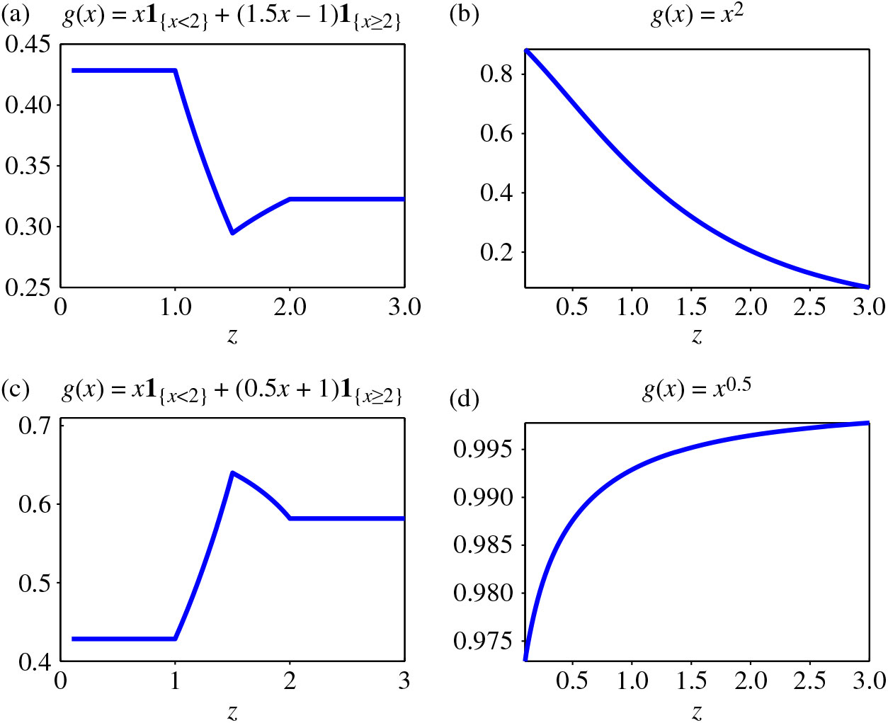
, in Figure 1(a)–(d) we plot the ratio H (z) defined in
 $$ ( 6 ) $$
with respect to z for
 $$x=0.5$$
and
 $$y=0.5$$
with
 $$s=1$$
,
 $$t=1.25$$
,
 $$\beta=0.75$$
, and
 $$g(x)=x
\mathbf{1}_{\{x\lt 2\}}+(1.5x-1)\mathbf{1}_{\{x\geq 2\}}$$
in (a) and
 $$g(x)=x
\mathbf{1}_{\{x\lt 2\}}+(0.5x+1)\mathbf{1}_{\{x\geq 2\}}$$
in (c), and with
 $$s=0.25$$
,
 $$t=1.75$$
,
 $$\beta=2$$
, and
 $$g(x)=x^2$$
in (b) and
 $$g(x)=x^{0.5}$$
in (d). This leads to
 $$A ( t ) -A ( s ) \simeq0.18$$
(DHR) for cases (a) and (c), and to
 $$A ( t ) -A ( s )
=3$$
(IHR) for cases (b) and (d). We observe from Figure 1 that H(z) decreases with z in case (b), whereas it increases in case (d). This is coherent with what could be expected from Proposition 4 whenever g is convex (case (b)) or concave (case (d)), under the IHR assumption for
 $$X_{t}-X_{s}$$
. Now, when
 $$X_{t}-X_{s}$$
is DHR, it can be seen from cases (a) and (c) in Figure 1 that the ratio H (z) is not monotonous with respect to z, neither for a convex function g (case (a)) nor for a concave function g (case (c)). Hence, it seems that nothing more can be said than the results of Proposition 4 in a general setting.
Plots of H(z) with respect to z (when
 $${X_t}\,k({t^\beta },1)$$
) for
 $$x=0.5$$
and
 $$y=0.5$$
with
 $$s=1$$
,
 $$t=1.25$$
, and
 $$\beta=0.75$$
in (a) and (c), and with
 $$s=0.25$$
,
 $$t=1.75$$
, and
 $$\beta=2$$
in (b) and (d) (with the function g defined above each plot); see Example 2.

We next look at a similar example to the previous one, now considering an inverse Gaussian process instead of a gamma process. Note that the inverse Gaussian distribution is known not to have a monotonic hazard rate in a general setting (that is, it is neither IHR nor DHR; see [6]) so that the conclusions of Proposition 4 do not apply in this case.
Example 3. Let
 $$A\colon \mathbb{R}_{+} \rightarrow\mathbb{R}_{+}$$
be a time-scaling function and let
 $$b>0$$
. Let
 $$(X_{t})_{t\geq 0}$$
be a nonhomogeneous inverse Gaussian process with mean function A(t) and rate parameter b (denoted by
 $${({X_t})_{t > 0}}\,ok(A( \cdot ),b)$$
). Then
 $$(X_{t})_{t\geq 0}$$
is a Lévy process such that each increment
 $$X_{t}-X_{s}$$
(with
 $$0\lt s\lt t$$
) is inverse Gaussian distributed
 $${ok( A ( t ) -A ( s ) ,b ) $$
, where the inverse Gaussian distribution
 $${ok} (a,b ) $$
(with
 $$a>0,b>0$$
) admits the PDF
 $$f(x)=\sqrt{\frac{b}{2\pi}}x^{-{3}/{2}}\exp\Big\{-\frac{b(x-a)^{2}}{2a^{2}x}
\Big\} \quad\text{for all } x > 0
$$
and the positive assumption holds. Letting
 $$A (t ) =t^{\beta}$$
and
 $$b=1$$
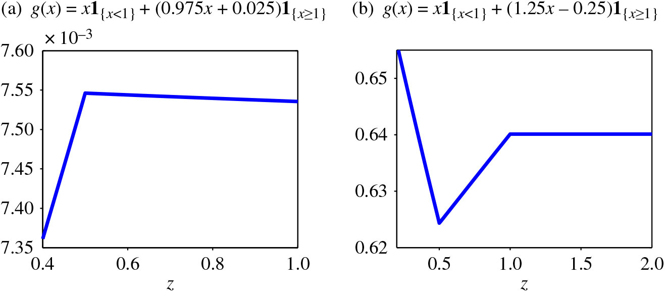
, in Figure 2(a) and (b) we plot the ratio H (z) defined in
 $$ ( 6 ) $$
with respect to z for
 $$x=0.5$$
and
 $$y=0.5$$
with
 $$s=1$$
,
 $$t=1.25$$
,
 $$\beta=0.95$$
(which leads to
 $$A(t)-A(s)\simeq 0.24$$
), and
 $$g(x)=x \mathbf{1}_{\{x\lt 1\}}+(0.975x+0.025)\mathbf{1}_{\{x\geq 1\}}$$
in (a), and with
 $$s=0.5$$
,
 $$t=1.5$$
,
 $$\beta=2$$
(which leads to
 $$A(t)-A(s)=2$$
), and
 $$g(x)=x \mathbf{1}_{\{x\lt 1\}}+(1.25x-0.25)\mathbf{1}_{\{x\geq 1\}}$$
in (b). In Figure 2 we observe that H(z) is not monotonic with respect to z neither when g is concave (case (a)) nor convex (case (b)). It is easy to check that in these two cases,
 $$X_{t}-X_{s}$$
is not IHR (nor DHR). The IHR assumption hence appears as necessary to derive the results in Proposition 4.
Plots of H(z) with respect to z (when
 $$X_{t}\sim {ok}(t^{\beta} , 1) $$
) for
 $$x=0.5$$
and
 $$y=0.5$$
with
 $$s=1$$
,
 $$t=1.25$$
, and
 $$\beta=0.95$$
in (a), and with
 $$s=0.5$$
,
 $$t=1.5$$
, and
 $$\beta=2$$
in (b) (with the function g defined above each plot); see Example 3.

Next we look at ageing properties (IHR/DHR) of an increment of a TR Lévy process.
Proposition 5. Let
 $$0\lt s\lt t$$
.
Assume that
$$X_{t}-X_{s}$$
is IHR and that g is convex. Then
$$ [
Z_{t}-Z_{s}\ \,\,|\, \ \, Z_{s}=z ] $$
is IHR.Assume that
$$X_{t}-X_{s}$$
is DHR and that g is concave. Then
$$ [
Z_{t}-Z_{s}\ \,\,|\, \ \, Z_{s}=z ] $$
is DHR.


Proof. We consider only the first point as the second point is similar. Let
 $$y\geq0$$
and z be fixed. We need to show that
 $$\begin{equation}
G ( x ) :\!= \frac{\overline{F}_{Z_{t}-Z_{s}\ \,\,|\, \ \, Z_{s}=z} (
x+y ) }{\overline{F}_{Z_{t}-Z_{s}\ \,\,|\, \ \, Z_{s}=z} ( x ) }
\label{eqn7}
\end{equation}
$$
decreases with respect to x. This can be proved in a similar way as for the proof of Proposition 4 and is therefore omitted.
Remark 3. Note that contrary to Proposition 4, the results in Proposition 5 do not require the positive assumption to hold. However, it is well known that DHR distributions have a bounded support from below (see, e.g. [Reference Barlow and Proschan2]), so that the second point is useless in case of a baseline Lévy process with
 $$\mathbb{R}$$
as support (such as a Wiener process).
The first point of Proposition 5 is now illustrated considering a Wiener process as a baseline Lévy process.
Example 4. Let
 $$ ( X_{t} ) _{t \ge 0}$$
be a time-scaled Wiener process with drift as defined in Example 1, where
 $${X_t}{\rm{ t}}({t^\beta },\sigma {t^\beta })$$
with
 $$\sigma=1$$
and
 $$\beta=0.75$$
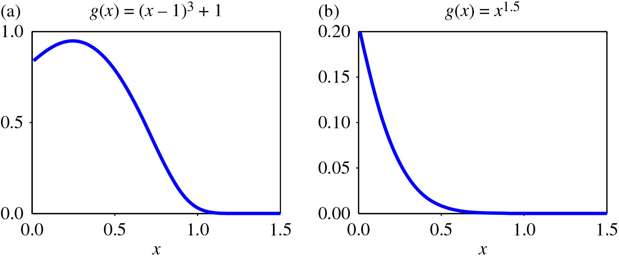
. In Figure 3(a) and (b) we plot the ratio G (x) defined in
 $$ ( 7 ) $$
with respect to x for
 $$y=0.5$$
,
 $$z=0.5$$
,
 $$s=1,$$
and
 $$t=1.25,$$
with
 $$g(x)=$$
 $$(x-1)^{3}+1$$
in (a) and with
 $$g(x)=x ^{1.5}$$
in (b). Recall from [3] that any normal random variable is IHR, so
 $$X_t-X_s$$
is IHR. In case (b) we see that G(x) is decreasing with respect to x. This is coherent with Proposition 5 based on the fact that g is convex. In case (a) the function g is neither convex nor concave and nothing can be said from Proposition 5. It can be observed that indeed G is not monotonic. This shows that the convexity/concavity assumption is required in Proposition 5 in order to derive the conditional IHR/DHR property of an increment.
Plots of G(x) with respect to x (when
 $${X_t} \sim {\rm{t}}({t^{0.75}},{t^{0.75}})$$
) for
 $$y=0.5$$
,
 $$z=0.5$$
,
 $$s=1,$$
and
 $$t=1.25,$$
with
 $$g(x)=(x-1)^{3}+1$$
in (a) and
 $$g(x)=x^{1.5}$$
in (b); see Example 3.

Remark 4. One may also be interested in the unconditional ageing property of
 $$Z_{t}-Z_{s}$$
. Actually,
 $$Z_{t}-Z_{s}$$
can be regarded as the mixture of
 $$[ Z_{t}-Z_{s}\ \,\,|\, \ \, Z_{s}=z] $$
with respect to the mixture distribution of
 $$Z_{s}$$
. It is well known that the mixture of DHR random variables is DHR. Thus, from the second point of Proposition 5, we can conclude that
 $$Z_{t}-Z_{s}$$
is DHR as soon as
 $$X_{t}-X_{s}$$
is DHR and g is concave. However, the mixture of IHR random variables is not necessarily IHR and nothing can be said about the IHR property of
 $$Z_{t}-Z_{s}$$
in general.
3.2 Influence of the current state on the future deterioration level
Proposition 6. Let
 $$0\lt s\lt t$$
. If
 $$X_{t}-X_{s}$$
is IHR (DHR) then
 $$[ Z_{t}\ \,\,|\, \ \, Z_{s}=z] $$
increases (decreases) in the hazard rate ordering as z increases, whatever g is.
Proof. We consider only the IHR case as the DHR case is similar. Let x and y be fixed (
 $$y\geq0$$
). We need to show that
 $$J(z): = {{{{\bar F}_{{Z_t}\;{\kern 1pt} {\kern 1pt} |{\kern 1pt} \;{\kern 1pt} {Z_s} = z}}(x + y)} \over {{{\bar F}_{{Z_t}\;{\kern 1pt} {\kern 1pt} |{\kern 1pt} \;{\kern 1pt} {Z_s} = z}}(x)}}$$
increases with respect to z, which can be shown similarly as in the proof of Proposition 4.
Proposition 7. Let
 $$0\lt s\lt t$$
. If
 $$X_{t}-X_{s}$$
is decreasing/increasing reverse hazard rate (DRHR/IRHR) then
 $$[ Z_{t}\ \,\,|\, \ \, Z_{s}=z] $$
decreases/increases in the reverse hazard rate ordering as z increases, whatever g is.
Proof. We consider only the DRHR case as the IRHR case is similar.
Let x and y be fixed (
 $$y\geq0$$
). We need to show that
 $$K(z): = {{{F_{{Z_t}\;{\kern 1pt} {\kern 1pt} |{\kern 1pt} \;{\kern 1pt} {Z_s} = z}}(x + y)} \over {{F_{{Z_t}\;{\kern 1pt} {\kern 1pt} |{\kern 1pt} \;{\kern 1pt} {Z_s} = z}}(x)}}$$
decreases with respect to z. Let
 $$z_{1}\leq z_{2}$$
. We have
 $$K ( z_{i} ) =\frac{F_{X_{t}-X_{s}} ( g ( x+y )
-g ( z_{i} ) ) }{F_{X_{t}-X_{s}} ( g ( x )
-g ( z_{i} ) ) }=\frac{F_{X_{t}-X_{s}} ( u+v_{i}
) }{\overline{F}_{X_{t}-X_{s}} ( v_{i} ) },
$$
with
 $$u=g ( x+y ) -g ( x ) \geq0 $$
and
 $$v_{i}=g (
x ) -g ( z_{i} ) $$
for
 $$i=1,2$$
.
As g is increasing, we have
 $$v_{1}\geq v_{2}$$
. Assume that
 $$X_{t}-X_{s}$$
is DRHR. Then
 $$K ( z_{1} ) =\frac{F_{X_{t}-X_{s}} ( u+v_{1} )
}{F_{X_{t}-X_{s}} ( v_{1} ) }\leq\frac{F_{X_{t}-X_{s}} (
u+v_{2} ) }{F_{X_{t}-X_{s}} ( v_{2} ) }=K (
z_{2} ) ,
$$
completing the proof.
Proposition 8. Let
 $$0\lt s\lt t$$
. If the PDF of
 $$X_{t}-X_{s}$$
is log-concave (log-convex) then
 $$[ Z_{t}\ \,\,|\, \ \, Z_{s}\,{=}\,z] $$
increases (decreases) in the likelihood ratio ordering as z increases, whatever g is.
Proof. We consider only the log-concave case as the log-convex case is similar. Let
 $$z_{1}\leq z_{2}$$
. We need to show that
 $${{f{X_t} - {X_s}\left( {u + h} \right)} \over {f{X_t} - {X_s}\left( {v + h} \right)}}$$
increases with respect to x. Based on the log-concavity of
 $$f_{X_{t}-X_{s}} $$
, we know that
 $${{{f_{{X_t} - {X_s}}}(u + h)} \over {{f_{{X_t} - {X_s}}}(v + h)}}$$
increases with respect to h whenever
 $$u\leq v$$
. Considering
 $$h=g (
x ) -g ( z_{2} ) $$
,
 $$u=0\leq v=g ( z_{2} )
-g ( z_{1} ) $$
, it follows that L(x) increases with respect to h and, hence, with respect to x, completing the proof.
4 Positive dependence properties
We now come to positive (negative) dependence properties and we first look at the dependence properties between the increments of a transformed Lévy process.
Proposition 9. Under the positive assumption, the following statements hold.
Assume that g is concave. Then, for all
$$t_0=0\lt t_{1}\lt \cdots\lt t_{n}$$
, the random vector
$$( Z_{t_{1}},Z_{t_{2}}-Z_{t_{1}},\ldots,Z_{t_{n}
}-Z_{t_{n-1} }) $$
is conditionally increasing in sequence (CIS), namely, (8)for all
$$\begin{align}
& [ Z_{t_{i}}-Z_{t_{i-1}}\ \,\,|\, \ \, Z_{t_{1}}=z_{1},Z_{t_{2}}-Z_{t_{1}}
=z_{2},\ldots,Z_{t_{i-1}}-Z_{t_{i-2}}=z_{i-1} ] \nonumber
\\
&\qquad \prec_{\rm st} [ Z_{t_{i}}-Z_{t_{i-1}}\ \,\,|\, \ \,
Z_{t_{1}}=z_{1}^{\prime},Z_{t_{2} }-Z_{t_{1}}=z_{2}^{\prime},
\ldots,Z_{t_{i-1}}-Z_{t_{i-2}}=z_{i-1}^{\prime } ]
\label{eqn8}\end{align}
$$
$$i\in \{ 2,\ldots,n \} $$
and all
$$z_{j}\leq
z_{j}^{\prime} $$
,
$$j\in \{ 1,\ldots,i-1 \} $$
; see, e.g. [8, Definition 5.3.22.].Assume that g is convex. Then, for all
$$t_0=0\lt t_{1}\lt \cdots\lt t_{n}$$
, the random vector
$$( Z_{t_{1}},Z_{t_{2}}-Z_{t_{1}},\ldots,Z_{t_{n}
}-Z_{t_{n-1}}) $$
is conditionally decreasing in sequence (CDS), namely, the inequality in (8) is reversed.


Proof. We consider only the concave case, as the convex case is similar. We need to show (8).
Based on the Markov property, we know that
 $$\begin{align*}
& [ Z_{t_{i}}-Z_{t_{i-1}}\ \,\,|\, \ \, Z_{t_{1}}=z_{1},Z_{t_{2}}-Z_{t_{1}}
=z_{2},\ldots,Z_{t_{i-1}}-Z_{t_{i-2}}=z_{i-1} ]
\\
&\qquad \,\stackrel{\text{I.D.}}{=}\, [ Z_{t_{i}}-Z_{t_{i-1}}\ \,\,|\, \ \, Z_{t_{i-1}} =z_{1:
i-1} ],
\end{align*}
$$
with
 $$z_{1\colon i-1}=\sum_{j=1}^{i-1}z_{j}.
$$
As
 $$z_{j}\leq z_{j}^{\prime}$$
,
 $$j\in \{ 1,\ldots,i-1 \} $$
, we also have
 $$z_{1: i-1}\leq z_{1: i-1}^{\prime}$$
(similar notation).
Owing to the second point of Lemma 1, we obtain
 $$ [ Z_{t_{i}}-Z_{t_{i-1}}\ \,\,|\, \ \, Z_{t_{i-1}}=z_{1:i-1} ] \prec_{\rm
st} [ Z_{t_{i}}-Z_{t_{i-1}}\ \,\,|\, \ \, Z_{t_{i-1}}=z_{1:i-1}^{\prime} ]
.
$$
Then
 $$( Z_{t_{1}},Z_{t_{2}}-Z_{t_{1}},\ldots,Z_{t_{n}}-Z_{t_{n-1} }) $$
is CIS.
Remark 5. As CIS is closed under marginalization (as a consequence of Theorem 3.10.19 in [20]), it follows that, when g is concave, the random vector
 $$ ( Z_{t_{1}},Z_{t_{3}}-Z_{t_{2}},\ldots
,Z_{t_{2n+1}}-Z_{t_{2n}} ) $$
is CIS. This shows that, when g is concave, the CIS property still holds for nonoverlapping but not necessarily consecutive intervals. However, to the best of the authors’ knowledge, CDS is not known to be closed under marginalization. The question hence remains open whether the CDS property holds for increments of a TR Lévy process over nonoverlapping intervals.
Remark 6. Let us recall that a random vector
 $${\boldsymbol{V}}=(V_1,V_2,\ldots,V_n)$$
is said to be (positively) associated if
 $$\begin{equation*}
\mathbb{E}[h({\boldsymbol{V}})w({\boldsymbol{V}})] \geq \mathbb{E}[h({\boldsymbol{V}})]\mathbb{E}[w({\boldsymbol{V}})]
\end{equation*}
$$
for all nondecreasing functions h and w such that
 $$\mathbb{E}[h({\boldsymbol{V}})]$$
,
 $$\mathbb{E}[w({\boldsymbol{V}})],$$
and
 $$\mathbb{E}[h({\boldsymbol{V}})w({\boldsymbol{V}})]$$
exist; see, e.g. [20]. Furthermore, a random vector
 $${\boldsymbol{V}}=(V_1,V_2,\ldots,V_n)$$
is said to be positive upper (lower) orthant dependent (PUOD/PLOD) if
 $$\begin{equation}
\mathbb{P} [ V_i> (\leq)\, v_i,\, i=1,2,\ldots,n ] \geq
\prod_{i=1}^{n} \mathbb{P} [V_i> (\leq)\, v_i ]
\label{eqn9}
\end{equation}
$$
for all
 $$v_i$$
,
 $$i=1,2,\ldots,n$$
. If the inequality ‘
 $$\geq$$
’ in ,≥- (9) is reversed, the random vector
 $${\boldsymbol{V}}=(V_1,V_2,\ldots,V_n)$$
is said to be negative upper (lower) orthant dependent (NUOD/NLOD). We recall that CIS implies association, which itself implies PUOD/PLOD properties; see, e.g. [8, Property 7.2.11]. The previous result hence shows that, when g is concave, the random vector
 $$(Z_{t_{1}},Z_{t_{2}}-Z_{t_{1} },\ldots,Z_{t_{n}}-Z_{t_{n-1}})$$
is associated, and, consequently, both PUOD and PLOD. As for negative dependence properties, it is known from [Reference Rinott and Samuel-Cahn21] that CDS implies an NLOD property. Then, if g is convex, the random vector
 $$ ( Z_{t_{1}},Z_{t_{2}}-Z_{t_{1}},\ldots,Z_{t_{n}}-Z_{t_{n-1}} )
$$
is NLOD. However, to the best of the authors’ knowledge, it seems that nothing else can be derived from the CDS property.
We now consider positive (negative) dependence properties for successive overall deterioration levels in a TR Lévy process.
Proposition 10. For all
 $$0\lt t_{1} \lt \cdots\lt t_{n}$$
, the random vector
 $$ (
Z_{t_{1}},Z_{t_{2} },\ldots,Z_{t_{n}} ) $$
is CIS, and, hence, associated and PUOD/PLOD, whatever g is.
Proof. We need to show that
 $$\begin{align*}
[ Z_{t_{i}}\ \,\,|\, \ \, Z_{t_{1}}=z_{1},Z_{t_{2}}=z_{2},\ldots,Z_{t_{i-1}}
=z_{i-1} ] \prec_{\rm st} [ Z_{t_{i}}\ \,\,|\, \ \,
Z_{t_{1}}=z_{1}^{\prime},Z_{t_{2}}
=z_{2}^{\prime},\ldots,Z_{t_{i-1}}=z_{i-1}^{\prime} ]
\end{align*}
$$
for all
 $$i\in \{ 2,\ldots,n \} $$
and all
 $$z_{j}\leq
z_{j}^{\prime} $$
,
 $$j\in \{ 1,\ldots,i-1 \} $$
, where we set
 $$t_{0}=0$$
and
 $$Z_{t_{0}}=0$$
.
Based on the Markov property, we know that
 $$ [ Z_{t_{i}}\ \,\,|\, \ \, Z_{t_{1}}=z_{1},Z_{t_{2}}=z_{2},\ldots,Z_{t_{i-1}}
=z_{i-1} ] \,\stackrel{\text{I.D.}}{=}\, [ Z_{t_{i}}\ \,\,|\, \ \, Z_{t_{i-1}} =z_{i-1} ],
$$
which stochastically increases with respect to
 $$z_{i-1}$$
, based on Lemma 1. This completes the proof.
Before going to the last positive (negative) dependence result, let us recall that a function
 $$f\colon \mathbb {R}^{n}\mapsto \mathbb {R}_{+}$$
is said to be multivariate totally positive of order 2 (MTP2) if
 $$f({\boldsymbol{x}})\,\, f({\boldsymbol{y}})\leq f({\boldsymbol{x}}\vee{\boldsymbol{y}})\,\, f({\boldsymbol{x}}\wedge{\boldsymbol{y}})
\quad\text{for all } {\boldsymbol{x}},\, {\boldsymbol{y}}\in \mathbb{R}^{n},
$$
where ‘
 $$\vee$$
’ and ‘
 $$\wedge$$
’ are the max and min componentwise operations, respectively. The function f is said to be multivariate reverse rule of order 2 (MRR2) when the previous inequality is reversed; see [Reference Karlin and Rinott15] and [Reference Karlin and Rinott16] for more details on these notions.
Proposition 11. Let
 $$t_{0}=0\lt t_{1}\lt\cdots\lt t_{n}$$
. If the PDF of
 $$X_{t_{i}}-X_{t_{i-1}}$$
is log-concave (log-convex) for each
 $$i\in \{ 1,\ldots,n \} $$
then
 $$ ( Z_{t_{1}},Z_{t_{2}} ,\ldots,Z_{t_{n}} ) $$
is MTP2 (MRR2), whatever g is.
Proof. We consider only the log-concave case, as the log-convex case is similar. We have
 $$f_{ ( Z_{t_{1}},Z_{t_{2}},\ldots,Z_{t_{n}} ) } ( z_{1}
,\ldots,z_{n} ) =\,f_{Z_{t_{1}}} ( z_{1} ) \prod_{i=2}
^{n-1}f_{Z_{t_{i}}\ \,\,|\, \ \, Z_{t_{i-1}}=z_{i-1}} ( z_{i} ) .
$$
Based on Proposition 8, we know that
 $$ [ Z_{t_{i}} \ \,\,|\, \ \,
Z_{t_{i-1}}=x_{i-1} ] \prec_{\rm lr} [ Z_{t_{i}}\ \,\,|\, \ \, Z_{t_{i-1}}
=z_{i-1} ] $$
for all
 $$x_{i-1}\leq z_{i-1}$$
so that
 $$f_{Z_{t_{i}}\ \,\,|\, \ \, Z_{t_{i-1}}=z_{i-1}} ( x_{i} )\, f_{Z_{t_{i}}
\ \,\,|\, \ \, Z_{t_{i-1}}=x_{i-1}} ( z_{i} ) \leq\, f_{Z_{t_{i}}\ \,\,|\, \ \,
Z_{t_{i-1} }=z_{i-1}} ( z_{i} )\, f_{Z_{t_{i}}\ \,\,|\, \ \,
Z_{t_{i-1}}=x_{i-1}} ( x_{i} )
$$
for all
 $$x_{i-1}\leq z_{i-1}$$
and
 $$x_{i}\leq z_{i}$$
. This shows that
 $$f_{Z_{t_{i}}\ \,\,|\, \ \, Z_{t_{i-1}}=z_{i-1}} ( z_{i} ) $$
is TP2 in
 $$ ( z_{i-1},z_{i} ) $$
and, hence, MTP2 as a function of
 $$ (
z_{1} ,\ldots,z_{n} ) $$
. Also,
 $$f_{Z_{t_{1}}} ( z_{1} ) $$
is MTP2 as it is a univariate function of
 $$ (
z_{1},\ldots,z_{n} ) $$
. As a product of MTP2 functions is MTP2,
 $$f_{ ( Z_{t_{1}},Z_{t_{2}} ,\ldots,Z_{t_{n}} ) } (
z_{1},\ldots,z_{n} ) $$
is hence MTP2.
Under the log-concavity assumption on the increments of the baseline Lévy process
 $$(X_t)_{t\geq 0}$$
, the successive deterioration levels of the TR Lévy process
 $$(Z_t)_{t\geq 0}$$
hence fulfills the MTP2 property, so that they are strongly positively dependent. (We recall that, among others, the MTP2 property implies CIS.) However, when the increments of the baseline Lévy process are log-convex, the successive deterioration levels of the TR Lévy process fulfill the MRR2 property, which is a negative dependence property. This was not necessarily expected, as from Proposition 10, this vector also exhibits CIS, which is a positive dependence property. These results are illustrated in the following example.
Example 5. Let
 $$g(x)=x^{1.5}$$
and
 $$X_{t}\sim k (t,1 )$$
. Then
 $$X_{t}-X_{s}\sim\, \,k ( t-s,1 )$$
for
 $$0\lt s\lt t$$
and if
 $$t-s \lt (\gt)1$$
, the PDF of
 $$X_{t}-X_{s}$$
is log-convex (log-concave); see, e.g. [19]. Two cases are considered:
 $$t_1=0.25 \lt t_2=1.2, x_2=1.5>y_2=1>x_1=0.25$$
and
 $$t_1=1.35 \lt t_2=2.75,x_2=3>y_2=2>x_1=1$$
. These cases respectively lead to log-convex and log-concave PDFs for both
 $$X_{t_{1}}$$
and
 $$X_{t_{2}}-X_{t_{1}}$$
. The function
 $$d_{(x_1,x_2,y_2)}(y_1)=\,f_{(Z_{t_1},Z_{t_2})}(x_1,x_2)\,f_{(Z_{t_1},
Z_{t_2})}(y_1,y_2)-\,f_{(Z_{t_1},Z_{t_2})}(x_1,y_2)\,f_{(Z_{t_1},Z_{t_2})}
(y_1,x_2)
$$
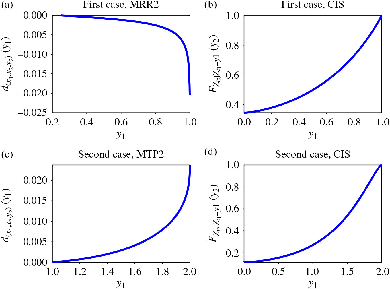
is plotted for
 $$y_1\in [x_1,y_2]$$
in Figures 4(a) and (c), whereas
 $$\bar{F}_{Z_{t_2}\ \,\,|\, \ \, Z_{t_1}=y_1}(y_2)$$
is plotted as a function of
 $$y_1$$
in Figures 4(b) and (d) for
 $$y_2=1$$
and
 $$y_2=2$$
, respectively. Figures 4(a) and (b) correspond to the first case, and
 $$(Z_{t_1},Z_{t_2})$$
is observed to be both MRR2 and CIS. Figures 4(c) and (d) correspond to the second case, and
 $$(Z_{t_1},Z_{t_2})$$
is observed to be both MTP2 and CIS. All figures are hence in coherence with what was expected from the previous results.
Plots of
 $$d_{(x_1,x_2,y_2)}(y_1)$$
and
 $$\bar{F}_{Z_{t_2}\ \,\,|\, \ \, Z_{t_1}=y_1} (y_2)$$
as a function of
 $$y_1$$
with
 $$(x_1,x_2,y_2)$$
fixed; see Example 5.

5 Stochastic monotonicity of increments
Proposition 12. Assume that the positive assumption holds, and let
 $$h>0$$
be fixed. Furthermore, assume that g is convex (concave) and that
 $$X_{t+h}-X_{t}$$
decreases (increases) in the sense of the usual stochastic order with respect to t. Then
 $$Z_{t+h}-Z_{t}$$
decreases (increases) in the sense of the usual stochastic order with respect to t (with
 $$h>0$$
fixed).
Proof. We consider only the convex case, as the concave case is similar. Let
 $$h
> 0$$
and
 $$x \geq 0$$
be fixed. For
 $$t \geq 0$$
, we have
 $$\mathbb{P} ( Z_{t+h}-Z_{t}>x ) =\mathbb{E} ( \varphi
_{t} ( Z_{t} ) )
$$
with
 $$\begin{align*}
\varphi_{t} ( z ) =\mathbb{P} ( Z_{t+h}-Z_{t}
> x\ \,\,|\, \ \, Z_{t}=z ) =\overline{F}_{X_{t+h}-X_{t}}
( g ( z+x ) -g ( z ) ).
\end{align*}
$$
Now let
 $$t_{1} \lt t_{2}$$
. Let us note that, under the positive assumption,
 $$X_{t_1}\leq X_{t_2}$$
and, hence,
 $$X_{t_1}\prec_{\rm st} X_{t_2}$$
. Also,
 $$X_{t_{1}+h}-X_{t_{1}}\succ_{st}X_{t_{2}+h}-X_{t_{2}}$$
by assumption. Then
 $$\varphi_{t_{1}}\geq\varphi_{t_{2}}$$
and
 $$\mathbb{P} ( Z_{t_{1}+h}-Z_{t_{1}}>x ) =\mathbb{E} (
\varphi_{t_{1}} ( Z_{t_{1}} ) ) \geq\mathbb{E} (
\varphi_{t_{2}} ( Z_{t_{1}} ) ) .
$$
As
 $$\varphi_{t_{2}} ( z ) $$
decreases with respect to z (because g is convex and
 $$x \geq0$$
) and as
 $$Z_{t_{1}}=g^{-1} (
X_{t_{1}} ) \prec_{\rm st}Z_{t_{2}}=g^{-1} ( X_{t_{2}} ) $$
(because
 $$X_{t_{1} }\prec_{\rm st}X_{t_{2}}$$
and
 $$g^{-1}$$
increases), it follows that
 $$\mathbb{E} ( \varphi_{t_{2}} ( Z_{t_{1}} )
) \geq\mathbb{E} ( \varphi_{t_{2}} ( Z_{t_{2}} )
) $$
and, consequently,
 $$\mathbb{E} ( \varphi_{t_{1}} ( Z_{t_{1}} ) )
\geq\mathbb{E} ( \varphi_{t_{2}} ( Z_{t_{2}} ) ),
$$
completing the proof.
Example 6. Let
 $${({X_t})_{t > 0}}{\rm{ ok}}(A( \cdot ),1)$$
. Considering the expression of the failure rate of an IG distribution given in [6, p.
463], it is easy to check that
 $${ok}(a,b)$$
increases in the hazard rate ordering when a increases with b fixed. Thus, if
 $$A ( \cdot ) $$
is convex (concave) then
 $$X_{t+h}-X_{t}$$
increases (decreases) in the hazard rate ordering and, hence, in the usual stochastic ordering [Reference Müller and Stoyan20]. We take
 $$A(t)=t^{\beta}$$
,
 $$g(x)=t^{\gamma}$$
,
 $$h=0.5$$
,
 $$x=0.5,$$
and the survival function
 $$\overline{F}_{Z_{t+h}-Z_{t}} ( x ) $$
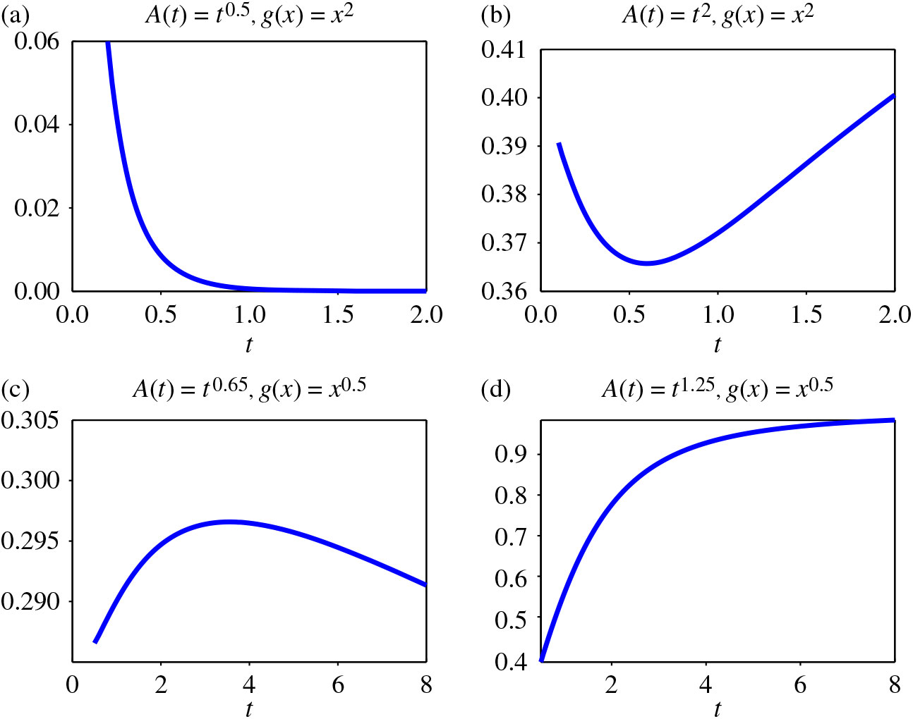
is plotted with respect to t in Figure 5(a)–(d) for
 $$\beta=0.5$$
and
 $$\gamma=2$$
in (a),
 $$\beta=\gamma=2$$
in (b),
 $$\beta=0.65$$
and
 $$\gamma=0.5$$
in (c), and
 $$\beta=1.25$$
and
 $$\gamma=0.5$$
in (d). Case (a) (case (d)) corresponds to the case where
 $$A ( \cdot )$$
is concave (convex) and
 $$g (
\cdot ) $$
is convex (concave). The results are coherent with what was expected from Proposition 12. Cases (b) and (c) correspond to the cases where
 $$A ( \cdot ) $$
and
 $$g ( \cdot ) $$
are both convex and both concave, respectively. As can be seen on the two plots,
 $$X_{t+h}-X_{t}$$
is not stochastically monotonous with respect to t and, hence, it seems that nothing more can be said than the results of Proposition 12 in a general setting.
Plots of
 $$\overline{F}_{Z_{t+0.5}-Z_{t}}(0.5)$$
with respect to t (when
 $$X_{t}\sim{ok}(t^{\beta},1) $$
) for
 $$g(x)=x^{\gamma}$$
with (a)
 $$\beta=0.5,\gamma=2$$
(b)
 $$\beta=\gamma=2$$
(c)
 $$\beta=0.65.\gamma=0.5,$$
and (d)
 $$\beta=1.25,\gamma=0.5$$
; see Example 6.

6 Stochastic comparison of two TR Lévy processes
Here we consider the stochastic comparison of two TR Lévy processes keeping the same baseline process or the same state function for both processes, which allows a better understanding of the influence of each item (baseline process/state function) on the behavior of the resulting TR Lévy process.
6.1 Common baseline process with different state functions
Proposition 13. Consider two processes
 $$ ( Z_{1t} ) _{t \ge 0}$$
and
 $$ (
Z_{2t} ) _{t \ge 0}$$
having a common baseline process
 $$(X_{t})_{t \ge 0}$$
and corresponding state functions
 $$g_{1}(x)$$
and
 $$g_{2}(x)$$
, respectively. Assume that the positive assumption holds for both processes.
If one among
$$g_{i}(x),\,i=1,2,$$
is concave and
$$g_{1}(z+x)-g_{1}(z)\leq
g_{2}(z+x)-g_{2}(z)$$
for all
$$z\geq0,~x>0$$
, then
$$Z_{1t}-Z_{1s}
\succ_{st}Z_{2t}-Z_{2s}$$
for any
$$0\leq s \lt t$$
.If one among
$$g_{i}(x)$$
,
$$i=1,2$$
, is convex and
$$g_{1}(z+x)-g_{1}(z)\ge g_{2}(z+x)-g_{2}(z)$$
, for all
$$z\geq0,~x>0$$
, then
$$Z_{1t}-Z_{1s}
\prec_{\rm st}Z_{2t}-Z_{2s}$$
, for any
$$0\leq s \lt t$$
.


Proof. We consider only the first point, as the second point is similar. As a first step, assume that
 $$g_{1}$$
is concave. Then, for any fixed
 $$x\geq0$$
,
 $$\overline{F}_{Z_{1t}-Z_{1s}\ \,\,|\, \ \, Z_{1s}
=z}(x)=\overline{F}_{X_{t}-X_{s}}(g_{1} (z+x)-g_{1}(z))
$$
is increasing in z. Furthermore, under the positive assumption,
 $$g_{1}(0)=g_{2}(0)=0$$
, which implies that
 $$\overline{F}_{Z_{1s}}(x)=\overline
{F}_{X_{s}}(g_{1}(x))\geq\overline{F}_{Z_{2s}}(x)= \overline{F}_{X_{s}}
(g_{2}(x))$$
,
 $$i=1,2$$
, and
 $$Z_{1s}\succ_{st}Z_{2s}$$
. Therefore,
 $$\begin{align*}
\overline{F}_{Z_{1t}-Z_{1s}}(x)=\mathbb{E}[\overline{F}_{X_{t}-
X_{s}}(g_{1} (Z_{1s}+x)-g_{1}(Z_{1s}))]
\geq\mathbb{E}[\overline{F}_{X_{t}-X_{s}}(g_{1}(Z_{2s}+x)
-g_{1}(Z_{2s}))].
\end{align*}
$$
Now, as
 $$g_{1}(z+x)-g_{1}(z)\leq g_{2}(z+x)-g_{2}(z)$$
by assumption, we obtain
 $$\begin{align*}
\overline{F}_{Z_{1t}-Z_{1s}}(x) \geq\mathbb{E}
[\overline{F}_{X_{t}-X_{s}}(g_{2}(Z_{2s}+x)-g_{2}(Z_{2s}))]
=\overline{F}_{Z_{2t}-Z_{2s}}(x).
\end{align*}
$$
As a second step, assume that
 $$g_{2}$$
is concave. Using similar arguments, we have
 $$\begin{align*}
\overline{F}_{Z_{1t}-Z_{1s}}(x) &
=\mathbb{E}[\overline{F}_{X_{t}-X_{s}}(g_{1} (Z_{1s}+x)-g_{1}(Z_{1s}))]
\\
& \geq\mathbb{E}[\overline{F}_{X_{t}-X_{s}}(g_{2}(Z_{1s}+x)-
g_{2}(Z_{1s}))]
\\
& \geq\mathbb{E}[\overline{F}_{X_{t}-X_{s}}(g_{2}(Z_{2s}+x)-
g_{2}(Z_{2s}))]
\\
& =\overline{F}_{Z_{2t}-Z_{2s}}(x).\tag*{\qedhere}
\end{align*}
$$
Proposition 14. Consider two processes
 $$ ( Z_{1t} ) _{t \ge 0}$$
and
 $$ (
Z_{2t} ) _{t \ge 0}$$
having a common baseline process
 $$(X_{t})_{t \ge 0}$$
and corresponding state functions
 $$g_{1}(x)$$
and
 $$g_{2}(x)$$
, respectively. Assume that the positive assumption holds for both processes, that
 $$X_{t}$$
is IHR, and that
 $$g_{2}-g_{1}$$
is nondecreasing. Then
 $$Z_{1t}\succ_{hr}Z_{2t}$$
for any
 $$t>0$$
.
Proof. Let
 $$\lambda_{X_{t}}$$
denote the hazard rate of
 $$X_{t}$$
. As
 $$g_1(0)=g_2(0)$$
under the positive assumption, we observe that
 $$\begin{align*}\\[-24pt]
r ( x ) & =\frac{{\overline{F}}_{Z_{1t}}(x)}
{{\overline{F}}_{Z_{2t}}
(x)}
\\
&=\frac{{\overline{F}}_{X_{t}}(g_{1}(x))}{{\overline{F}}_{X_{t}}
(g_{2}(x))}
\\
&=\frac{\exp \{ -\int_{0}^{g_{1}(x)}\lambda_{X_{t}}(u)\,\mathrm{d} u \} }
{\exp \{ -\int_{0}^{g_{2}(x)}\lambda_{X_{t}}(u)\,\mathrm{d} u \} }
\\&
=\exp \bigg\{ \int_{0}^{g_{2}(x)-g_{1} ( x ) }\lambda_{X_{t}
}(v+g_{1} ( x ) )\,\mathrm{d} v \bigg\} .
\end{align*}
$$
As
 $$g_{2}-g_{1}$$
is nondecreasing with
 $$g_{1}(0)={g_{2}(0)}=0$$
, then
 $$g_{2}(x)-g_{1} ( x ) \geq0$$
for all
 $$x\geq0$$
. As
 $$g_{1}$$
and
 $$\lambda_{X_{t}}$$
are also nondecreasing (because
 $$X_{t}$$
is IHR), it follows that r (x) is nondecreasing, completing the proof.
6.2 Common state function with different baseline processes
Proposition 15. Consider two processes
 $$ ( Z_{1t} ) _{t \ge 0}$$
and
 $$ (
Z_{2t} ) _{t \ge 0}$$
having a common state function g(x) and corresponding baseline processes
 $$(X_{1t})_{t \ge 0}$$
and
 $$(X_{2t}
)_{t \ge 0}$$
, respectively. Assume that the positive assumption holds for both processes and that the common state function g is concave. Let
 $$0\leq s \lt t$$
. Then, if
 $$X_{1t}-X_{1s}\prec_{\rm st}X_{2t}-X_{2s}$$
and
 $$X_{1s}\prec_{\rm st}X_{2s}$$
, we have
 $$Z_{1t}-Z_{1s}\prec_{\rm
st}Z_{2t}-Z_{2s}$$
.
Proof. Observe that, as
 $$X_{1t}-X_{1s}\prec_{\rm st}X_{2t}-X_{2s}$$
,
 $$\begin{align*}
\overline{F}_{Z_{1t}-Z_{1s}\ \,\,|\, \ \, Z_{1s}=z}(x) &
=\overline{F}_{X_{1t}-X_{1s}} (x)(g(z+x)-g(z))
\\
& \leq\overline{F}_{X_{2t}-X_{2s}}(x)(g(z+x)-g(z))
\\
& =\overline{F}_{Z_{2t}-Z_{2s}\ \,\,|\, \ \, Z_{2s}=z}(x)
\end{align*}
$$
for all
 $$x,z\geq0$$
. Furthermore, as
 $$X_{1s}\prec_{\rm st} X_{2s}$$
and
 $$g^{-1}$$
increases,
 $$Z_{1s}=g^{-1}(X_{1}(s))\prec_{\rm
st}Z_{2s}=g^{-1}(X_{2}(s))$$
. Also, as g is concave,
 $$\overline{F}_{Z_{1t}-Z_{1s}\ \,\,|\, \ \, Z_{1s}=z}(x)$$
is increasing in z for all
 $$x\geq0$$
. Thus,
 $$\begin{align*}
\overline{F}_{Z_{1t}-Z_{1s}}(x) & =\int_{0}^{\infty}
\overline{F}_{Z_{1t}-Z_{1s} \ \,\,|\, \ \, Z_{1s}=z}(x)\,f_{Z_{1s}}(z)\,\mathrm{d} z
\\
& \leq\int_{0}^{\infty}\overline{F}_{Z_{1t}-Z_{1s}\ \,\,|\, \ \,
Z_{1s}=z}(x)\,f_{Z_{2s}} (z)\,\mathrm{d} z
\\
& \leq\int_{0}^{\infty}\overline{F}_{Z_{2t}-Z_{2s}\ \,\,|\, \ \,
Z_{2s}=z}(x)\,f_{Z_{2s}} (z)\,\mathrm{d} z
\\
& =\overline{F}_{Z_{2t}-Z_{2s}}(x).\tag*{\qedhere}
\end{align*}
$$
Note that similar results would not be valid for a convex function g. This is illustrated in Example 7.
Example 7. Let
 $$X_{it}\sim k ( (t+1)^{\beta_{i}}-1,1 ), i=1,2,$$
with
 $$\beta _{1}=1$$
and
 $$\beta_{2}=2$$
. Then, it can be checked that
 $$X_{1s}\prec_{\rm st} X_{2s}$$
and
 $$X_{1t}-X_{1s}\prec_{\rm st}X_{2t}-X_{2s}$$
for all
 $$0\leq s\leq t$$
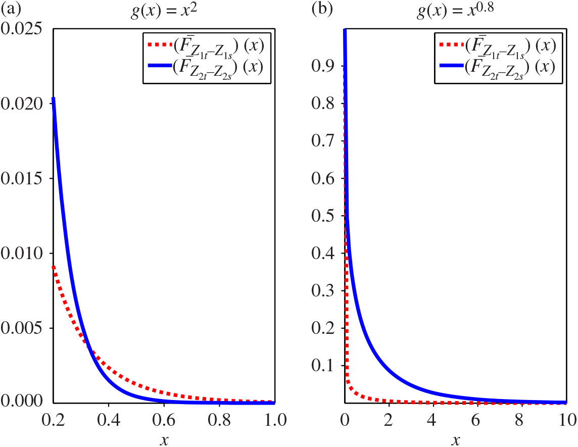
. In Figure 6(a) and (b) we plot the survival functions of
 $$Z_{it}-Z_{is}$$
,
 $$i=1,2,$$
with respect to x for
 $$s=4.5, t=4.53,$$
and
 $$g(x)=x^{2}$$
in (a), and for
 $$s=3, t=3.03,$$
and
 $$g(x)=x^{0.8}$$
in (b). It can be seen that, as expected from Proposition 15, when g is concave (case (b)), we have
 $$Z_{1t}-Z_{1s}\prec_{\rm st}Z_{2t}-Z_{2s}$$
. However, in the convex case (case (a)),
 $$Z_{1t}-Z_{1s}$$
and
 $$Z_{2t}-Z_{2s}$$
are not comparable with respect to the usual stochastic order.
Survival functions of
 $$Z_{it}-Z_{is}$$
,
 $$i=1,2,$$
with respect to x; see Example 7.

7 Conclusion and perspectives
In this paper we proposed a new class of state-dependent wear models, which includes the transformed gamma process proposed in [Reference Giorgio, Guida and Pulcini12] and the classical geometric Brownian motion. Transformed Lévy processes allowed us to overcome the independent increments property of standard Lévy processes, and, hence, enlarge their modeling ability. They however remain tractable Markov processes. Several results provided some insight into the influence of the current state of a TR Lévy process on its future, which typically differs according to the (log-)concavity/convexity property of the state function. Some positive (negative) dependence properties have also been highlighted for the increments of deterioration and for the overall deterioration levels of a TR Lévy process, which here again are highly dependent on the (log-)concavity/convexity property of the state function. In the case of a (log-)concave state function, we observed strong positive dependence properties (such as MTP2). This seems to be in coherence with wear phenomena where the rate of deterioration increases over time. When the state function exhibits a (log-)convex property, we observed that some positive and negative dependence properties can hold on the same process (see the end of Section 5). Also, there remain open questions about negative dependence properties (see, e.g. Remarks 5 and 6). This is coherent with the previous literature where it has already been observed that negative dependence properties are much more involved than positive dependence properties; see, e.g. [Reference Block, Savits and Shaked4] or [Reference Karlin and Rinott16] where the authors exhibited a three-dimensional MRR2 vector with a two-dimensional MTP2 vector as margin.
Clearly, there remains much work to do on the new TR Lévy process. For instance, even if a first study can be found in [Reference Giorgio, Guida and Pulcini12] in a specific parametric setting, generic estimation procedures still require development.
Acknowledgements
The corresponding author of this paper, Ji Hwan Cha, was supported by the National Research Foundation of Korea (NRF) grant funded by the Korea government (MSIP) (no. 2019R1A2B5B02069500). Ji Hwan Cha’s work was also supported by the Basic Science Research Program through the National Research Foundation of Korea (NRF) funded by the Ministry of Education (grant number 2019R1A6A1A11051177).