

Usury – the idea that riskless loans ought not require a return in excess of the initial funds granted – was an important part of medieval Catholic religious doctrine. The church was more accepting of partnerships and of profit from bearing risk. Clearly, it was important to distinguish between loans and partnerships. This turned out to be surprisingly difficult.
Fischer Black and Myron Scholes (Reference BLACK and SCHOLES1973) show that options and risk-free debt can be seen as capital market building blocks. With put-call parity we know that firm ownership can be equally embodied in the stock or the bonds.Footnote 1 So who owns the firm, stockholders or creditors? Similar ambiguity could be said to exist between a homeowner and the mortgage holder. In this article we use modern asset pricing analysis, including put-call parity, to show that such ambiguity played a role in medieval businessmen's efforts to circumvent the Catholic Church's usury restrictions. That ambiguity created fertile ground for a financial innovation, the triple contract, that allowed them to accomplish a kind of regulatory arbitrage. We also show that medieval clerics and merchants appear to have had at least an intuitive grasp of put-call parity, and that this insight shaped the church's approach to medieval business contracts, and usury, nearly five centuries before put-call parity was described in the scholarly literature.
Put-call parity refers to a result obtained by Stoll (Reference STOLL1969). Stoll shows that C – P = S – PVK, where S refers to a specific underlying asset, C and P are European call and put options (respectively) on that asset, with common exercise price K and expiration date, and PVK refers to the present value of the strike price K discounted at the risk-free rate. Usually, we view the stock as an ownership position, particularly since stockholders exercise many of the rights of owners. The ambiguity stems from our ability to also view the stock as a kind of call option on the firm, subject to outstanding debt as the strike price. Until the call is exercised, the stockholder does not yet own the stock, the creditor does.
Of course, options occur in many relationships, and are not always recognized as options. For example, options are similar to insurance commitments. An auto insurance policy confers the right to exchange your car (after an accident) for a specific payment. The same could be said of a put option on the car, with an exercise price equal to the payment.
Discussions of contractual form in this context – clerics and merchants concerned with usury – may illustrate more general phenomena as well, among them: regulatory capture, regulatory arbitrage and financial innovation. Koyama (Reference KOYAMA2010) argued that the increasingly complex contracts developed during the Middle Ages were clerical and merchant responses to usury restrictions.Footnote 2 These were cases of regulatory capture, as described by Stigler (Reference STIGLER1971).
Regulation may be actively sought by an industry, or it may be thrust upon it. The central thesis of this paper is that, as a rule, regulation is acquired by the industry and is designed and operated primarily for its benefit. There are regulations whose net effects upon the regulated industry are undeniably onerous; a simple example is the differentially heavy taxation of the industry's product (whiskey, playing cards). These onerous regulations, however, are exceptional and can be explained by the same theory that explains beneficial (we may call it ‘acquired’) regulation. (1971, p. 3)
In a nutshell, regulatory capture refers to when a regulatory regime comes to act more in the interests of the regulated industry than of the public at large. Regulatory arbitrage is a bit different. As Knoll (Reference KNOLL2005) put it:
There is a strong incentive for financial innovators to disaggregate and rebundle cash flows in order to avoid prohibited or disadvantaged transactions. When this occurs, the innovator can charge a premium for its product, at least until others catch on, that reflects the saving. Such innovations are commonly referred to as tax or regulatory arbitrage. (2005, p. 65)
Some historical examples of regulatory arbitrage have already been documented.Footnote 3 For example, Knoll (Reference KNOLL1994) uses put-call parity to illustrate and document how modern mortgage law was shaped in medieval England by the insight that usury restrictions could be circumvented by suitably structuring loan transactions. Further, Knoll (Reference KNOLL2008), following Ellickson and Thorland (Reference ELLICKSON and THORLAND1995), documents how usury restrictions were also circumvented in ancient Mesopotamia.
In regulatory capture then, in general, the regulations are operated for the benefit of the regulated. In regulatory arbitrage, the regulations are circumvented by the regulated. While both might apply, the triple contract appears to be more an example of regulatory arbitrage than of regulatory capture.
Development of the triple contract may also illustrate market contestability as described by Baumol, Panzer and Willig (Reference BAUMOL, PANZAR and WILLIG1982), who show that sunk costs can represent an entry barrier. By avoiding the contractual complexity described by Koyama, the triple contract lowers that entry barrier. And as noted by Bergier (Reference BERGIER1979), for centuries, banking in Europe had been dominated by the Italians, until the end of the fifteenth century. Thereafter, Germans, Britons, Belgians and Dutch had a much greater role. The triple contract may have been part of that change by allowing German bankers operating out of Augsburg, such as the Fugger, to effectively contest the market for banking services, thereby undermining the dominance of the Italians.
The development of the triple contract may have had even wider significance. The timing of the very public and very controversial defense of the triple contract (see below), occurring just a few years before the onset of the Reformation and involving some of the same parties – this seems a very curious coincidence.
This article makes two main contributions. First, we show that the development and structure of the triple contract can be understood by the application of modern asset pricing analysis. Second, we show that medieval clerical scholars and merchants appear to have had at least an intuitive grasp of put-call parity, and that this insight shaped the Catholic Church's approach to medieval business contracts, and usury. In the balance of this article, we review the historical background and scholastic discussion of usury, then some of what is known about the medieval business contracts at issue, the clerical response, and the triple contract, with illustrating diagrams. We then discuss the problem presented by the triple contract, and its resolution.
I
Clerical scholars (scholastics) and merchants have long been concerned about usury. Some of their earliest writings addressed the substance of usury. As business activity increased during the commercial revolution of the eleventh to thirteenth centuries, it was also necessary to discuss the form of usurious contracts. Even so, banking and finance were well established among Italians well before the fifteenth century. As noted by Oberman:
The discrepancy between the church's prohibition of usury and routine business practice had apparently long since found a satisfactory solution as far as the canon lawyers in the Italian financial centres were concerned. Yet merchants in the south German commercial capitals found themselves faced with a grave question of conscience at the beginning of the 16th century. Explaining why they could not have adopted the Italian solutions is as difficult as the intellectual history of the period is complex. (1981: 121)Footnote 4
By the fifteenth century, some scholastics, particularly in Germany, shifted their focus from contractual form and substance to the intent of the contracting parties. This shift may have created an opening for the triple contract as a legitimate form of investment.
Usury doctrine, the prohibition of the taking of interest, was an important part of the Judeo-Christian tradition from antiquity. Indeed, concerns about debt and usury are present in many cultures and long before Abraham, at least as far back as ancient Mesopotamia, as illustrated by the Code of Hammurabi (which specified a maximum interest rate of 34 percent), roughly 4,000 years ago. In some cultures, such as that of the ancient Babylonians, the approach was to limit permitted interest rates. At other times, the approach was one or more debt holidays, when pre-existing debts were voided, such as among the early Hebrews, Greeks and Babylonians.Footnote 5 According to Graeber (Reference GRAEBER2012), the concern in many of these contexts was with debt slavery – for communities not far above ‘subsistence’ levels, a crop failure or similar event would force consumption loans that would be difficult to ever pay off, especially with high interest rates. The borrower could be induced to sell off more and more of their assets: land, livestock, even children and wives into slavery to pay off the debt. Eventually, the borrower too could be reduced to slavery.
For still other groups, such as the early Catholic Church, and also Islam, the approach was to prohibit interest entirely. To the Catholic Church, money was ‘barren’, and its use should not produce a profit without bearing risk. The Catholic view toward usury was based on multiple passages of the Old and New Testaments, as well as Aristotle, but is particularly informed by the Gospel of Luke,Footnote 6 further elaborated in the writings of the scholastics, but also shown in popular culture such as Shakespeare's Merchant of Venice.
The earliest church pronouncements against usury, shortly after the Council of Nicaea, were directed against clerical lending. Only later, under Charlemagne, was usury forbidden generally. Note that usury and loans were not always clearly defined. Usury was considered an example of the sin of avarice. Rubin (Reference RUBIN2009) argued that lay Catholic usury restrictions began to be taken even more seriously after the church committed to providing social insurance to the poor. He noted that the provision of social insurance created moral hazard, inducing some folks to borrow more. Limiting the interest rate would discourage such borrowing by reducing willingness to lend. A common element to such lending and debt is that the loans typically were used to pay taxes or for consumption, such as after a crop failure. They were not income producing or productive loans.
Even so, certain types of business contracts were already in wide use in the Roman Empire even before the Council of Nicaea defined the New Testament in ad 325. When early medieval clerics including the scholastics sought to explain and defend the prohibition on interest they tended to accept Roman institutions as licit. As Noonan (Reference NOONAN1957), notes:
The Scholastics [were] disciples of the Roman Law, and from the earliest revival of Medieval culture, canon law and moral theology are impregnated with the concepts of Roman jurisprudence. The Scholastics [did] not accept this jurisprudence unmodified, but they [did] accept it in substance, and well before the Renaissance regal jurists appealed to it, they established its basic concepts in a realm which concerned practical life most closely. (1957, p. 2)Footnote 7
As disciples of Roman law, the scholastics were more lawyers than economists, and were in fact trained to pay close attention to the form of a contract or other relation, at least as much as to the economic substance of that relation.
II
Among the Roman contracts considered by the scholastics were the Sea Loan, and the Societas (or partnership). The Roman Sea Loan (Foenus Nauticum) was similar to the Ancient Greek ‘Maritime Loans’, which in turn may have been derived from Babylonian sea loans.Footnote 8 Sea Loans were generally recognized as especially risky due to shipwrecks and piracy among other factors. With the Sea Loan, the traveling merchant had no obligation to repay in the event of a loss at sea.
According to Jones (Reference JONES and Whaples2008), the Romans allowed an array of interest rates that were set according to the purpose of the loan. In the Lex Unicaria of 88 bc, Roman law allowed interest rates of up to 12 percent for Sea Loans, 8 percent for business loans, 6 percent for non-business loans, and 4 percent for farmers and distinguished persons. In this sense, 12 percent for a Sea Loan would be, for a Roman, ‘licit usury’. The extra interest on Sea Loans was thought to be compensation for risk (Jones Reference JONES and Whaples2008).
Noonan (Reference NOONAN1957, pp. 134–5) argues that Sea Loans were subject to some contention. Sea Loans were allowed to charge an explicit yield – for Rome, double the otherwise legal interest rate. Sea Loans were widely used in medieval Italy, particularly during the twelfth century. However, early in the thirteenth century, Pope Gregory IX in the decretal ‘Naviganti’ (1234) ruled that Sea Loans were (illicit) usury. During and after the thirteenth century, other contract forms may have become more widely used, perhaps because of Naviganti.
The Societas was also a widely used business form in the Roman world:
The Societas, or Partnership, was a normal form of commercial organization throughout the Roman world; and it enters scholastic thought largely in the form given it by Roman law. A Societas, according to the Digest [of Ulpian] is the union by two or more persons of their money or skill for a common purpose, usually profit … Although a partnership in which one partner is entirely freed from risk of his capital is indistinguishable in effect from a loan, the Roman law treats a loan as formally distinct from this contract. The great change in the early Scholastic notion of partnership is that such a riskless partnership will be treated as a usurious loan. (Noonan Reference NOONAN1957, pp. 133–4)
Under the Romans, the Societas could take a variety of forms, being a sort of general purpose partnership structure, including partnerships where some parties bore little or no risk. Under the scholastics, the latter were considered loans. According to Noonan, referring to the Societas:
In this contract, money or goods are loaned to a ship-owner, the creditor assuming the risks of his debtor while the money or goods are actually at sea. If a shipwreck occurs and the property is lost, the debtor will not be liable in any way to return the loan. Once the voyage is completed, however, the borrower trades at his own risk, and if he loses the loan through commercial misfortune, he must still repay the lender… Roman law, however, does not assimilate the case with partnership, but treats it strictly as a kind of licit usury; and the canonists and Scholastics follow the sharp discrimination between it as a loan, and the normal partnership. (Noonan Reference NOONAN1957, pp. 134–5)
Among early Scholastics, the Societas was mentioned in the eleventh century by Ivo of Chartres, who distinguished loans, where usury may occur, from lawful partnerships, or Societas. Following Ivo, the assumption of risk was thought to distinguish lawful investment in a partnership from an illicit loan. Catholic teaching on the topic became more elaborate during the later eleventh century.
Noonan ascribes this elaboration to several factors, including the revival of trade at that time. It became apparent that usury on business loans could not be so easily condemned as due to greed or avarice. Instead, clerics such as St Anselm began to suggest that usury was similar to robbery, and was thus an instance of sin against justice (Noonan Reference NOONAN1957, pp. 15–17, 134–42). Concerning this revival of trade, Glaeser and Scheinkman (Reference GLAESER and SCHEINKMAN1998) develop a model of interest restrictions and usury laws. They conclude that interest restrictions will become tighter when inequality is high and impermanent. That seems a good description of the conditions in the mercantile city states of southern Europe as the trade-driven ‘commercial revolution’ made some households fabulously wealthy while ruining others.
Despite the Carolingian Renaissance, the economy of western Europe is thought to have contracted for several more centuries after the fall of the Western Roman Empire. Around ad 1000, the level of economic activity apparently bottomed out (Lopez Reference LOPEZ1971, p. 32). In the eleventh to thirteenth centuries, the Mediterranean part of the western European economy began to grow, particularly as evidenced by the trade-driven prosperity of the northern Italian city states, such as Amalfi, Florence, Genoa, Milan, Pisa and Venice (Lopez Reference LOPEZ1971: 71–2). With growth came increasing concern with usury on the part of church leaders. It is worth noting that church leaders did not always distinguish between business and consumption loans.
Even as the Societas and Sea Loans came into increasingly common use, scholastics struggled to clearly distinguish why the Societas was acceptable, and Sea Loans were not. Perhaps the clearest statement is attributed to St Thomas Aquinas (around 1265):
He who commits his money to a merchant or craftsman by means of some kind of partnership does not transfer the ownership of his money to him, but it remains his; so that at his risk the merchant trades, or the craftsman works, with it; and therefore he can licitly seek part of the profit thence coming as from his own property. (Noonan Reference NOONAN1957, p. 143)
Even so, scholastics continued to debate the nature of usury, and sought to clarify earlier pronouncements well into the eighteenth century.
A particular type of partnership, the Commenda (called Colleganza in Venice) came into wide use across Europe during the thirteenth century, perhaps in part as a response to concerns about usury (Lopez Reference LOPEZ1971, p. 76). On the other hand, rather than being a response to concerns about usury, Gonzalez de Lara (Reference GONZALEZ DE LARA2006), argues that changing contract choice in Venice was driven by changing institutional conditions, evidently near the end of the twelfth century: ‘Institutional arrangements that enhanced the state's ability to verify information led the transition from the Sea Loan (a debt-like contract) to the Commenda (an equity-like contract).’ While Gonzalez de Lara argues that usury doctrine did not play a large role in shaping contract form in Venice, Venice may have been an exception. Before Venice became independent, for a time it was administratively part of the Eastern Roman Empire, and therefore subject to the Eastern Orthodox Church, and so may have found it easier to ignore the Roman Church. Other Italian commercial centers may have been more strongly affected by papal concerns.
The origin of the Commenda is not entirely clear. Udovitch (Reference UDOVITCH1962), argues that the Commenda was similar to an older Islamic business form, the Qirad. The Qirad, by its origins, and as a contract where both parties bore some risk, would also have satisfied church concerns about usury. According to Pryor (Reference PRYOR1977), the origins of the Commenda, that is, the commercial tradition from which it arose, are less clear.Footnote 9
Whatever its origin, the Commenda is said to have facilitated substantial capital investment in trade. One possible consequence – in the late thirteenth and fourteenth centuries, Venice may have had the highest per capita income of any city in the world. The Commenda is also interesting for our purposes because it may have been a precursor to the ‘triple contract’, which we discuss in more detail below.
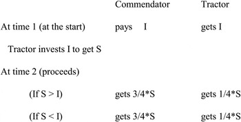
The Commenda came in two main varieties - ‘unilateral’ and ‘bilateral’. The bilateral form was sometimes also called the ‘Societas Maris’. In a unilateral Commenda, a fund provider, called a commendator, provides funds for a traveling partner, called a tractor, who would take the funds in pursuit of trading opportunity, with more or less direction and advice from the commendator. The commendator would stay home. The tractor would provide their skills and labor. On return, the tractor would give an accounting. If the proceeds exceeded the original commendator's investment, the value of the latter would be returned. In addition, the excess would be divided, 3/4 for the commendator, 1/4 for the tractor. If the proceeds fell short of the original investment, the commendator would get the balance, but would have no further claim against the tractor.
Over time, tractors might build up their own funds, and wish to join with a commendator to fund a venture. If the commendator provided 2/3 of the funds, and the tractor provided 1/3 of the funds, and the venture was profitable, the surplus would be divided evenly. This was called the bilateral Commenda. If different ratios of funds were available, merchants could draw up two Commendae, one unilateral, and one bilateral, to allocate funds and profits (de Roover Reference DE ROOVER1941). A given tractor would normally represent multiple commendators in a given voyage. According to Gonzalez de Lara (citing Lane Reference LANE1973), ‘A typical (ship) cargo probably represented the stakes of something like a hundred investors who had confided sums of various amounts to more than a dozen traveling merchants’ (Gonzalez de Lara Reference GONZALEZ DE LARA2006, p. 7).
Note that both the Sea Loan and the Commenda allow no obligation to repay the investment on the part of the traveling partner in the event of loss at sea. That is, at sea, both the Sea Loan and the Commenda look like partnerships. One difference is that with the Sea Loan, the traveling partner still bears liability for the investment from other types of risk – such as due to adverse price movements. Under the Commenda, the insurance is more comprehensive – applying to the whole of the venture, so that any financial losses are borne entirely by the commendator.Footnote 10
While the Commenda remained a mainstay of commerce for centuries, we also see the development of third-party maritime insurance during the fourteenth century, probably originating in or around Genoa (Nelli Reference NELLI1972; see also de Roover Reference DE ROOVER1945). Initially, it was not clear how clerics would view insurance. Early examples of the Genoan form of insurance were structured as a ‘fake sale’. Generally, insurers were other merchants – specialty insurers had not yet arisen. An insurer merchant would agree to buy the cargo or goods, but not pay or take delivery. A premium might be exchanged ‘under the table’. If the cargo got to its destination, the ‘sale’ documents would be set aside. If shipwreck or similar event destroyed the cargo, payment for the ‘sale’ would be completed. The Florentine form, where there is an explicit premium, became the norm later, as it remains today (Van Doosselaere Reference VAN DOOSSELAERE2009: ch. 5).
Early insurance records are sparse. However, Van Doosselaere (Reference VAN DOOSSELAERE2009) acquired and studied a large trove of notarial documents from Genoa for the period 1154 to 1440. Along with Sea Loans, Commenda and some other kinds of contracts, numerous maritime insurance contracts are recorded. He found that many of the insurance transactions were quite small, and were merchants insuring other merchants, often in a reciprocal way.
Van Doosselaere also showed that despite considerable activity, insurance underwriting was not particularly profitable. Based on his data, it was found that some merchants lost money underwriting, and others barely broke even.Footnote 11 While discounting diversification as a motive, Van Doosselaere interpreted this as a device to create class solidarity among the ruling elite clans of traders, during a period of political strife within Genoa.Footnote 12
We suspect other motives. If these insurance contracts are viewed as options, it would make sense that they might not make much money. First, a long call portfolio would be expected to have high risk and expected return. A short call portfolio would be expected to lose money. However, it would be a mistake to consider a short call portfolio in isolation. Typically, short calls are combined with a long position in the underlying assets to create a covered call portfolio – a low risk, with low but positive expected return position. Second, recall that options trading is a zero sum game. If merchants are reciprocally insuring each other, the expected return may well be close to zero. Third, the science of insurance underwriting had not yet developed. Merchants could not have been very confident that the insurance/options were priced right. Use of reciprocal insurance relations would reduce exposure to mispricing and allow diversification while also allowing merchants to adjust their exposure to specific risks, despite possible concerns about usury.
III
Note that already with the Sea Loan and the Commenda, and even more so with insurance, there is ambiguity about the relationship between commendator and tractor. Earlier scholastics, like Ivo of Chartres and Aquinas, had argued that ownership was indicated by exposure to risk of loss. Is the commendator an investor in a partnership – hence an owner entitled to an excess return – or a lender to an investor, or both? If the commendator is essentially a lender, as Naviganti concluded with the Sea loan, usury is a concern. If the commendator is only an investor, usury is not an issue. Similarly, is the tractor an investor alongside the commendator, or a borrower, potentially participating in usury? Can either party remain an investor in that sense if the risk of loss is borne by another party, an insurer? These issues will become only more acute with the development of the triple contract.
Despite the absence of a known Roman prototype, among scholastics, Laurentius de Ridolfis argued in 1403 that insurance was licit, and was not usury, because no loan was present. Other clerics joined in, on similar reasoning. Only one minor cleric writing late in the fifteenth century argued that insurance was usurious (Noonan Reference NOONAN1957, pp. 202–3). However, we will find that once insurance is accepted as ‘licit’, the distinction between legitimate partnerships and illegitimate loans begins to break down and usury doctrine with it.Footnote 13
Late in the fifteenth century, some scholastics did reconsider insurance in conjunction with other contracts. Recall that Ivo of Chartres, St Thomas Aquinas and most scholastics who followed them had used the incidence of risk to distinguish a usurious loan from a partnership. In 1485, Angelo Carletti, Vicar General of the Franciscans, argued that if you invest in a partnership, but your capital is guaranteed by your partner, and your partner will also pay you an additional sum at his discretion, then this is usury. We should note that in this context, the phrase ‘at his discretion’ may have been a bit of a subterfuge. If the contract was generally or explicitly understood to have required such a payment, that would surely mark it as usurious (Noonan Reference NOONAN1957, pp. 204–5). Our understanding of this situation is that under the conditions of repeated contracting among a small group of merchants, the discretionary ‘additional sum’ would be increasingly, effectively, required.
We can rephrase Carletti's statement in modern terms as: if (as commendator) you invest in a partnership, but acquire insurance (a put option) on your investment from the partner/tractor, while you give up some of the potential for future gain (a call option) to the partner/tractor, you have recreated a loan, which would be usurious. Clearly, Angelo Carletti understood that an equity investment, plus a put, minus a call, would approximate a loan, with interest. In terms of put-call parity: S + P – C = PVK.
Since, by combining a simple partnership or Commenda, ‘capital insurance’ and a discretionary sum that will resemble a short call option, this comes close to reconstructing a recourse loan paying an additional sum ‘x’, Carletti is right. Then he throws a curve ball. Carletti argues that if you could insure your capital with a third party rather than your partner, you could still licitly profit from the partnership. Perhaps he intended to preserve a role for third-party insurance. However, by treating third-party insurance as different from insurance by your partner/tractor, he still undermined the longstanding link between ownership and the risk of loss and the right to a return (Noonan Reference NOONAN1957, pp. 204–5). In an active insurance market, merchants could readily insure each other's ventures, as the third-party insurers. According to Van Doosselaere, that was already happening in Genoa for maritime insurance.
According to Oberman, Carletti's insights were extended by Gabriel Biel and Conrad Summenhart, theology professors at the University of Tübingen. For Biel and Summenhart, the form of the contract was no longer decisive, the intent of the participants was what mattered:
At this juncture, Summenhart entered the debate armed with his own arguments. He began by demonstrating that the assumption of risk was no requisite characteristic of a legitimate investment partnership. Normally, the person possessing capital must also accept the risks of the financial venture, but he also has ways to insure himself against risk. Risk then cannot be an essential component of a valid contract. The crucial factor is not risk but the intention of the lender or investor. From the outside it is impossible to distinguish a risk free partnership from usury even when the moneylenders intention is not usurious. Only a knowledgeable reader can determine the lender's intent since that intent determines the wording of the contract. In usury the capital is relinquished to the borrower whereas in a genuine partnership (fraternitas), the borrower receives a share in ownership so that both parties to the contract have a stake in the capital. (Oberman Reference OBERMAN1981, pp. 135–6)Footnote 14
The culmination of medieval contract development is the ‘triple contract’. We see the first possible references to the triple contract in the fifteenth century. Hunt and Murray (Reference HUNT and MURRAY1999) claim that the triple contract was developed around 1460, and consisted of three parts: a partnership, plus insurance of the principal invested against loss, plus a third insurance-like contract, insuring the tractor that the commendator will not ask for more than a given fixed amount from the tractor (Hunt and Murray Reference HUNT and MURRAY1999, p. 243).Footnote 15 According to Noonan, Angelo Carletti discusses something similar in 1485, but a close reading of Noonan suggests that Carletti is referring to insured contracts, but not necessarily the triple contract. Nor is it clear whether Carletti was discussing a real or hypothetical contract. In any case, in 1514 and 1515, the triple contract was very publicly defended by John Eck, a prominent theologian.
John Eck achieved fame for defending the licitness of the triple contract in debates with theologians in Bologna and Vienna. In this, he was actively supported by the Fugger banking house, who were reported to be heavily dependent on funds raised from a form of triple contract that resembles a bank deposit. The Fugger were also actively involved in financing the church and the sale of ‘indulgences’. One of Eck's allies in this controversy, Sebastion Ilsung of Augsburg, is reported by Wurm (Reference WURM1997, p. 67) to have said that the triple contract was used almost throughout christendom. Also, according to Wurm, Eck himself said that the contract had been in use in Augsburg for more than 40 years. Eck went on to greater fame as the point man in a public debate with Martin Luther, shortly before the latter finally broke with the Catholic Church, over issues such as the sale of indulgences. For more on this topic, see Rowan (Reference ROWAN1987).
According to Noonan, Eck saw the triple contract as:
-
(1) An ordinary partnership; plus
-
(2) a second contract of insurance of the principal, in which insurance is given in return for an assignment of the future probable gain from the partnership; plus
-
(3) a third contract by which an uncertain future gain is sold for a lesser certain gain.
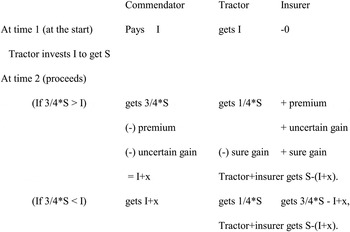
We can see, in this formulation of the first two, the same combination that Angelo Carletti saw as usurious. The third element reinforces the loan-like quality of the triple contract, as will be seen when we diagram it below. Depending on one's interpretation of these descriptions, the third element can be either a call option, or a straddle or a spread. The first two elements create something between a partnership and a loan with a kink. The third element smooths out the kink (see below) and completes the resemblance to a loan.
If we view the triple contract in terms of options rather than insurance, from the perspective of the commendator, it would appear as a partnership, plus a long put, plus a short call. There is some uncertainty about the implied strike price, since the put strike may have been the initial investment, or somewhat above that, and the call strike is possibly 5 percent above the initial investment. As long as these two strike prices were the same, the corresponding equation would be: S + P – C = ? Under put call parity, S + P – C = PVK.
That is, the triple contract would effectively be a loan, with interest. If the strike prices differ, the triple contract is not quite a loan, but it is very close. Note, that nothing about the triple contract requires the interest rate to be 5 percent. In that sense, the German ‘5 percent contract’ is a special case of the triple contract.
IV
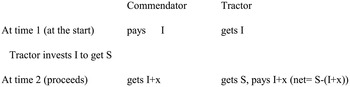
It may be useful to consider modern option pricing payoff diagrams to illustrate these relations. First consider a simple recourse loan. Under such a loan, the commendator pays I, and the tractor contributes his labor. The payoff S goes to the tractor, subject to the need to pay back the loan. Let I be the amount invested, S be the value of the resulting venture, x is any additional payment to the commendator at the conclusion of the venture.
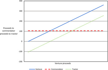
In Diagram 1, the payoff plotting receipts against S would be a flat line for the commendator, corresponding to the loan. The tractor receives a diagonal line passing into positive space at S = I + x. Of course, a recourse loan would have the problem that the tractor, or his estate, would have to pay even if the venture failed or even if he did not survive. According to Gonzalez de Lara, such loans were normally collateralized. Otherwise, given the extreme sanctions applied to bankruptcy during this period, that could be problematic.

Recourse loan

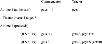
Now consider a non-recourse loan (Diagram 2). For such a loan, the lender promises – insures – that they will make no claim beyond the proceeds of the venture. Under such a loan, the inputs are the same, but the commendator will receive the loan repayment (=I + x), minus a put option with strike price (I + x). The insurance amounts to giving the put option to the tractor/borrower. The tractor will receive the put on the venture, plus the venture minus the loan (=S – (I + x) + Put). If S > (I + x), the put will not be exercised and the tractor will have S – (I + x). If S < (I + x), the tractor will exercise the put, and have nil. This is also equivalent to a long call with strike price (I + x). That is, S– (I + x) + Put = Call. The commendator's payoff could also be represented as a long position in the venture with a short call – a covered call. That is, Loan – Put = Venture – Call. These are both ways to express put-call parity.

Non-recourse loan

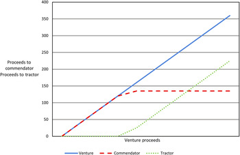
For a non-recourse loan, the payoff to the commendator would look like a loan minus a put, or a covered call on the venture – rising diagonally until S = I + x, at which point it becomes flat. Unless motivated by Christian charity, the commendator would expect a substantial x to compensate for having retained the downside risk but not upside potential, as illustrated in Table A1. The tractor's payoff would be the corresponding long call on the venture (or a long put on the loan), rising diagonally from where S = I + x. The tractor would have less risk and less return than with a recourse loan, but would still face a risky payoff.
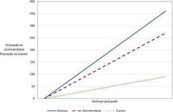
Now consider a simple partnership (Diagram 3). Under a simple partnership such as a Societas, the commendator pays I, the tractor adds his labor. If we assume for purposes of comparison that the same ratio applies here as to a Commenda, then at maturity, 3/4 of S goes to the commendator, and 1/4 of S goes to the tractor. Of course, this is not ideal – a tractor could go away and promptly return to collect 1/4 S. The Commenda solves that problem. Under the Commenda, the commendator receives repayment first, plus 3/4 of the surplus beyond repayment of the initial investment.

Simple partnership

For a simple partnership, the payoff diagram to the commendator is a diagonal line with slope 3/4*S. The tractor gets a payoff of slope 1/4*S. There is less risk here for the tractor than a loan, but the return is less as well. As noted above, there is a potential agency problem.
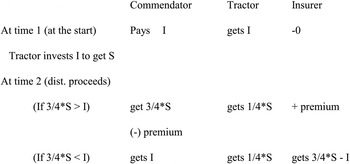
Now consider a partnership with insurance of the principal (Diagram 4). The insurer might be a third party, or the tractor. If the latter, this would address the agency problem above. With insurance, the payoff to the commendator would be I if 3/4*S < I, and would be 3/4*S if 3/4*S > I.

Partnership with principal insurance

Partnerships with principal insurance produce a kink in the payoffs. The slope of the commendator's payoff increases where I = S. The slope of the tractor's payoff, assuming they are also the insurer, decreases where I = S (see below).
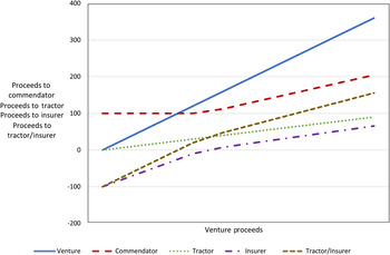
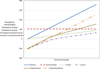
Recall, the triple contract (Diagram 5) consists of a partnership + insurance of principal – uncertain gain + smaller sure gain. It was presented as a partnership with insurance. In fact, to the commendator, the two insurance parts, like the two options they resemble, convert the whole to what is effectively a recourse loan. To the tractor, it remains a partnership, unless they take up the other side of the two insurance parts.

Triple contract (partnership with principal insurance less uncertain gain plus sure smaller gain)

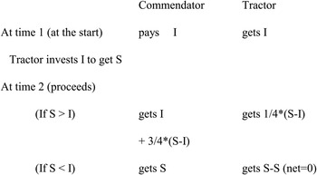
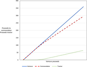
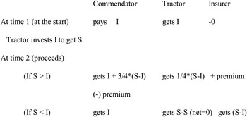
With a Commenda (Diagram 6), the initial investment is repaid first, and then the excess is divided, 3/4 to the commendator, and 1/4 to the tractor. For the commendator, the payoff diagram is a diagonal line until S = I + x, at which point the slope shifts down to 3/4. In terms of the payoff diagram, the difference between a simple partnership and a Commenda is a trapazoid like shape similar to the payoff from a bull call spread. The commendator receives 1/4*S up to (I + x) + 1/4*(I + x)*(S-(I + x)) more than under the simple partnership. Put differently, up to S = I + x, the Commenda looks like a non-recourse loan. Beyond S = I + x, the Commenda looks like a partnership. The tractor has less risk, and less return.

Commenda

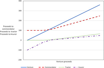
Now add investment ‘insurance’ to the Commenda (Diagram 7). The insurance underwriter sells a put on the venture to the commendator, with strike price (I), in exchange for some of the potential gain (S – I). The latter is a call option. The commendator now has a protective put on the venture, similar to a recourse loan, paying I, but also with some upside potential. That is, when the commendator sells a call and buys a put, he has reconstructed what begins to look like a recourse loan. So who would buy such a call? Recall, in Genoa, by the thirteenth century, there was an active market in third-party insurance.

Commenda with insurance of principal

Addition of insurance to the Commenda reverses the kink for the commendator. If the tractor is also the insurer, their payoff begins to resemble that of a non-recourse loan again.
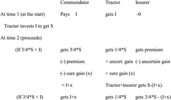
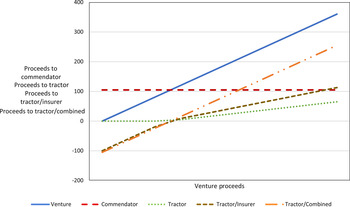
Finally, we can add an exchange of an uncertain gain for a smaller sure gain. If the tractor takes the opposite side of that too, we have again constructed a triple contract, and closely mimicked a recourse loan (Diagram 8).

Triple contract (Commenda with principal insurance less uncertain gain plus sure smaller gain)

V
As can be seen in Figures 5 and 8 or Tables A2 and A3, the triple contract essentially reconstructs the cashflows associated with a recourse loan. As such, if there is interest, one might conclude there is usury. However, because the scholastics had already accepted partnerships, including the Commenda, as well as insurance in connection with these partnerships, they could not conclude that without reversing themselves on prior decisions. As noted above, in 1514 and 1515, in a series of major defenses of the triple contract before the law faculties of the universities of Bologna and Vienna, Eck triumphed. The law faculties concluded that the triple contract was licit (Noonan Reference NOONAN1957, pp. 208–12).
One might ask whether the triumph of the triple contract was an example of regulatory capture, regulatory arbitrage, or both. There is some evidence for both. It is well known that during this period, prominent merchant families such as the Medici often placed one or more sons in the church, while the others pursued the family business. One might conjecture that clerical commentators might have been smoothing the way for their merchant siblings. That's a topic for another paper. It is also worth noting that the church was by this time reliant on the Fugger bank for loans and funds transfers around western Europe. On the other hand, Carletti's comments indicate that there was also resistance to such contracts within the church. Finally, given prior acceptance of commendae, and insurance, they really were in a box – suggesting regulatory arbitrage.
One might also ask, why Eck? Why south Germany? And why in the early sixteenth century rather than earlier or later? Neither the occasion for the debate nor Johannes Eck's participation in it were purely academic. Certainly, the shift in clerical/theological emphasis from the form and substance of the contract, as exemplified by Carletti, to the intent of the contracting parties, as exemplified by Biel and Summenhart, laid the groundwork for the triple contract. Likewise, it is worth noting that as a scholar, Eck followed in the latter's footsteps (Oberman Reference OBERMAN1981, p. 129). As observed by Oberman: ‘Eck's victory (at Bologna) represented a triumph not only for one of (the University of) Ingolstadt's professors, but for all the recent German university foundations, including Tübingen where Biel and Summenhart had done the spadework for Eck's success.’
In the later part of the fifteenth century, several south German Imperial cities, of which Nuremberg and Augsburg were the most important, took on an increasingly important role in financing silver and copper mining and commerce within the region, and diverse ventures elsewhere. Nuremberg particularly financed local kings princes and nobles, but was reported to have held back from financing Habsburg loans because they were regarded as too risky.
However, after 1474, when the Medici pulled out of Nuremberg, the Fuggers of Augsburg began to take on the business of the Roman Curia. From the fourteenth century, Nuremberg bankers had financed lending by offering investments to ‘silent partners’. These investments were called Komandite, which is a kind of ‘limited liability company’. If the Nuremberg banker's own investment ventures did poorly, the risks were shared by the silent partners. By contrast ‘fixed-rate deposits’, which were widely regarded as usurious, were not used much in Nuremberg (Wurm Reference WURM1997: 41–55).
Within a few years, besides the church, the Fuggers would also be financing Habsburg activities. Augsburg came to prominence somewhat later than Nuremberg, but rose rapidly during the later part of the fifteenth century, driven in part by new developments in silver and copper mining, very generous mineral concessions from local rulers, and also the willingness to finance Habsburg lending. Another distinguishing feature of the Augsburg houses was greater willingness to take on leverage, and to accept ‘fixed-rate deposits’.Footnote 16
The timing of the controversy may have been provoked by the death in 1509 of Melchior von Mechau, Cardinal of Brixen, and subsequent litigation over his estate (Duggan Reference DUGGAN1983). Eck's participation in the controversy was prompted by Dr Conrad Peutinger, town clerk of Augsburg, and chief publicist for the large trading firms there, including the Fugger. Peutinger urged Eck to defend the threefold (triple) contract against charges that it was usurious. According to Rowan, ‘Much of the capital of the major Augsburg firms derived from deposit contracts paying a fixed annual interest rate, usually five percent’ (1987, p. 111).Footnote 17 In fact, Eck's activity was substantially financed by Fugger banking interests.
The death of the cardinal, Melchior von Mechau, revealed a substantial investment in the Fugger bank, variously described as a ‘silent partnership’ (Wurm Reference WURM1997)Footnote 18 and a deposit (Rowan Reference ROWAN1987, p. 111). There followed protracted litigation between the church in Rome, the Fuggers and various third parties over the disposition of the estate. Had the timing been slightly different, or had the Fuggers been compelled to immediately turn over the proceeds, the claim might have bankrupted the Fugger bank. The Mechau estate amounted to 30 percent of the Fugger ‘deposit’ base. The Fugger interest was to play for time, which they did while raising funds elsewhere. Thereafter, several prominent Upper German academic and clerical commentators
launched an attack on fixed interest contracts and large scale cartels… By the start of the second decade of the [sixteenth] century, attacks on the financing methods of large firms were being launched with telling effect at several Imperial diets, and legislation was being formulated to limit the amount of capital which could be held by business concerns operating in the Empire. (Rowan Reference ROWAN1987, p. 111)Footnote 19
Johannes Eck's response to Peutinger's urgings included three essays in 1514 and 1515, ‘Treatise on Usurious Contracts’, ‘The Counsel of Johannes Eck on the Five Percent Contract’ and the ‘Treatise on the Five Percent Contract’. These analyses supported a publicity campaign, ‘fronted by Eck, backed by Peutinger's letters, and floated on Fugger monetary, logistical and political support’ (Rowan Reference ROWAN1987, p. 112). These, together with Eck's triumph in Bologna, gave the Fugger the cover they needed to continue to raise funds that looked like deposits, but were called investments.
Two generations later, in 1560, the Jesuits took up the fight again, arguing that the triple contract was indeed usury. Debate continued for decades, until finally in 1581, the general congregation of Jesuits, meeting in Rome, concluded that while taking 5 percent interest on a loan was usury, the triple contract yielding 5 percent was not (Noonan Reference NOONAN1957, pp. 212–17). By this time, the Protestant Reformation had greatly reduced the significance of the Catholic Church's position. Any merchant or prince unhappy with such conclusions would just have one more reason to switch sides.
VI
In this article, we have reviewed the history of medieval business contracting, and applied the logic of put-call parity to explain the development of the triple contract and its relation to church teachings on usury. The triple contract recreated a loan in a form that the church could not prohibit without contradicting itself. In theological discussions it is clear that from Angelo Carletti onward, writing in the late fifteenth century, the scholastics understood that the triple contract effectively recreated a loan. They evidently understood put-call parity. Had an equivalent explicit loan been considered, it surely would have been ruled illicit. In the form of the triple contract, the scholastics were in a box. So, they accepted the contract while rejecting its equivalent. As for businessmen, by this time, the House of Fugger, and other Augsburg banking houses were routinely financing loans to princes by taking ‘5 percent contracts’ from money centers such as Antwerp and Augsburg. It made perfect sense for the Fugger to finance Eck if his arguments would allow them to claim that instead of taking illicit deposits, they were making licit triple contracts. Put-call parity, the modern understanding that an equity investment plus a put option, minus a call option with the same expiration and strike price is effectively a loan, was understood by clerics and financial market participants nearly 500 hundred years before Stoll described it. Some parts of financial engineering are not so new after all.
Appendix
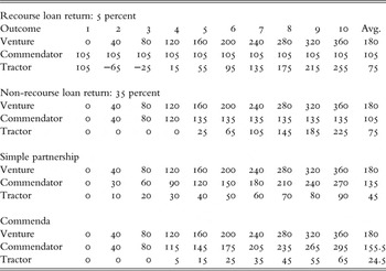
Here we illustrate some basic medieval contracts. For simplicity, following Commenda terminology, the provider of funds to be invested is called the commendator. The merchant who will use those funds in trade is called the tractor. In all cases, we assume 100 units of funds are provided, and consider a venture that can produce a range of outcomes, from abject failure (proceeds = 0), to substantial profit (proceeds = 360).
A recourse loan, assuming good collateral, allows the commendator a safe 105 units for a 5 percent return. A non-recourse loan, such as a Sea Loan, might occur when the tractor has no other assets. This exposes the commendator to substantial risk of loss. For these numbers, to achieve the same average 105, he'd have to charge 35 percent over the life of the venture. Sea Loans were ruled usurious in the thirteenth century.
A partnership is another form. Following the convention with Commenda, we assume the commendator will claim 3/4 of any proceeds, leaving 1/4 to the tractor. Note that the tractor gains even if the venture is a disappointment. The tractor has much less incentive to take risks than the commendator. A Commenda addresses this, so that the tractor gets nothing until the commendator is fully compensated for their investment.
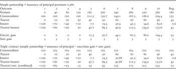
In Table A2 we illustrate some basic medieval contracts as modified by insurance ideas. As with Table A1, the provider of funds to be invested is called the commendator. The merchant who will use those funds in trade is called the tractor. In all cases, we assume 100 units of funds are provided, and consider a venture that can produce a range of outcomes, from abject failure (proceeds = 0), to substantial profit (proceeds = 360).
Illustration of some basic medieval contracts

Illustration of a partnership modified by insurance

Table A2 shows a partnership modified by insurance of the principal. Various interpretations are possible, but my understanding is that this insurance was not paid by a specific premium before the fact, but instead was paid with a predetermined fraction of the proceeds, paid after the fact. The result is that only successful outcomes pay the insurance. Given the probabilities of the various outcomes, that fraction can be quite high. We do know that early insurance was not very profitable, so I solved for the fraction that caused the insurance cash flows to break even. For these numbers, that fraction is 38.6 percent. Note that all cash flows occur at the same time, so there is no need to discount them. The next two lines capture the third part of the triple contract as described by Johannes Eck, ‘sale of an uncertain gain for a lesser certain gain’. Note that when these are combined with a simple partnership and insurance of the principal, we have reproduced the cash flows of the recourse loan. In this sense, the triple contract is a formally a partnership, but effectively a loan.
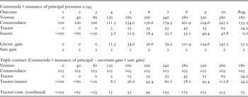
In Table A3 we illustrate how the Commenda is modified by insurance ideas. As with Tables A1 and A2, the provider of funds to be invested is called the commendator. The merchant who will use those funds in trade is called the tractor. In all cases, we assume 100 units of funds are provided, and consider a venture that can produce a range of outcomes, from abject failure (proceeds = 0), to substantial profit (proceeds = 360).
Illustration of a Commenda modified by insurance

Table A3 shows a Commenda modified by insurance of the principal. Various interpretations are possible, but my understanding is that this insurance was not paid by a specific premium before the fact, but instead was paid with a predetermined fraction of the proceeds, paid after the fact. The result is that only successful outcomes pay the insurance. Given the probabilities of the various outcomes, that fraction can be quite high. We do know that early insurance was not very profitable, so I solved for the fraction that caused the insurance cash flows to break even. Note that all cash flows occur at the same time, so there is no need to discount them. For these numbers, that fraction is 24.5 percent. The next two lines capture the third part of the triple contract as described by Johannes Eck, ‘sale of an uncertain gain for a lesser certain gain’. Note that when combined with a Commenda and insurance of the principal, we have reproduced the cash flows of the recourse loan. In this sense, the triple contract may formally be a Commenda, but effectively a loan. Initially, I was under the impression that the triple contract evolved from the Commenda, but as we saw with Table 2, that need not have been the case – the triple contract could also have evolved from the ordinary partnership.