


Impact Statement
This article demonstrates the value of integrating remote sensing, administrative data, interdisciplinary data from the physical and social sciences, and machine learning tools for the remote detection of illegal deforestation in Brazil, showing how data science approaches can assist government agencies to more safely and effectively prevent illegal deforestation and environmental degradation.
1. Introduction
Environmental crimes in Brazil include mining, the trafficking of plant and animal species, and illegal deforestation to convert land for cattle ranching, soy production, and logging for the black market in lumber (Boekhout van Solinge, Reference Boekhout van Solinge2010; Boekhout van Solinge, Reference Boekhout van Solinge2014; Skidmore et al., Reference Skidmore, Moffette, Rausch, Christie, Munger and Gibbs2021; Ministério do Meio Ambiente e Mudança do Clima, 2025). Detecting these crimes is important for several reasons, including the health of the environment, especially the Amazon biome, as well as broader social harms that result from environmental degradation (Carpio-Domínguez, Reference Carpio-Domínguez and Henry2024). Most deforestation in the region is illegal (1, 272) and is increasing: the period 2016–2020 showed almost twice as much deforestation as in comparable time spans from 2001 to 2005 or 2006 to 2010 (da Silva et al., Reference da Silva, Lopes and Santos2023a), and the first half of 2025 marked a record-breaking surge in deforestation (Berti, Reference Berti2025). Environmental crimes are often closely connected to violence and criminal networks, including persistent evasion of authorities and oversight (Carvalho et al., Reference Carvalho, Mustin, Hilário, Vasconcelos, Eilers and Fearnside2019), so improving detection of these crimes is also important to combat corruption and organized crime, and to reduce lawlessness and insecurity in the region (Alston et al., Reference Alston, Libecap and Mueller2000; Muggah, Reference Muggah2023; Muggah and Smith, Reference Muggah and Smith2024). Further, much of the violence and evasion that accompanies environmental crimes occurs in rural areas at the frontiers of government attention and regulation, so-called “brown areas” where the law is absent (O’Donnell, Reference O’Donnell2001; Carvalho et al., Reference Carvalho, Mustin, Hilário, Vasconcelos, Eilers and Fearnside2019), and thus where safety is a concern, so improvements to remote methods offer a way to monitor environmental degradation with lower personal risks.
Measuring environmental crimes is challenging, just as with other criminal behavior, in part due to the illicit, clandestine nature of the activity and the active efforts of those involved to remain hidden and hard to detect. Further, environmental crimes connected to deforestation, for example, illegal logging, are the kind of “gray” or “para-criminal” activity that is ingrained in regular, legal flows of economic activity that help camouflage the illegality (Vigh and Sausdal, Reference Vigh and Sausdal2025).
Yet, embargoes—legal liens on parcels of land for illegal environmental activity on the property—provide a way to identify locations where the government has already documented at least some of these crimes. Studies have leveraged these data to study compliance with embargoes (Silva et al., Reference Silva, Vieira, Galbraith, Potapov, M. Rivero, Lima, S. Pimentel and Adami2022) and changes in environmental enforcement over time (Nunes et al., Reference Nunes, Soares-Filho, Oliveira, Veloso, Schmitt, Van der Hoff, Assis, Costa, Börner, Ribeiro, Rajão, de Oliveira and Costa2024). However, while other administrative data have been incorporated into efforts to detect illegal deforestation (Ribeiro et al., Reference Ribeiro, De Souza Mendes, Singh and Heilmayr2024), to our knowledge, the data on embargoes have not. This study leverages information about these embargo locations to predict other, yet-unidentified locations of environmental crimes. This process complements existing efforts to improve government effectiveness in forest enforcement (Silva et al., Reference Silva, Vieira, Galbraith, Potapov, M. Rivero, Lima, S. Pimentel and Adami2022; Nunes et al., Reference Nunes, Soares-Filho, Oliveira, Veloso, Schmitt, Van der Hoff, Assis, Costa, Börner, Ribeiro, Rajão, de Oliveira and Costa2024).
The approach proceeds in three steps. First, using public, administrative data on embargoes, we identify documented locations of environmental crimes, focusing only on illegal logging and deforestation in the Legal Amazon, permitting us to isolate this one type of environmental crime within a key defined region. Second, we merge this information with data on a wide, interdisciplinary range of potential explanatory factors, including features of the physical environment from satellite imagery, as well as demographic, social, economic, political, and public safety attributes at each location. This varied combination of explanatory factors speaks to the call for interdisciplinary, multicausal, “multifactorial” approaches to illegal deforestation (Carpio-Domínguez, Reference Carpio-Domínguez and Henry2024). Third, we divide the data into training and testing subsets of the data, and train a series of models. The random forest (RF) model performs best, and we interpret this model in a series of steps, moving from a black box to a more understandable, explainable result consistent with interpretable machine learning (Doshi-Velez and Kim, Reference Doshi-Velez and Kim2017; Miller, Reference Miller2019; Molnar, Reference Molnar2025). The combination of remote sensing, administrative and interdisciplinary data, and machine learning responds to calls for greater use of remote sensing in monitoring illegal deforestation (Thompson and Magrath, Reference Thompson and Magrath2021; Ribeiro et al., Reference Ribeiro, De Souza Mendes, Singh and Heilmayr2024), and complements efforts to build data infrastructure on forests and pair these data with machine learning (Ouaknine et al., Reference Ouaknine, Kattenborn, Laliberté and Rolnick2025). The approach can be extended to detecting other environmental crimes and illicit behavior, in Brazil and elsewhere.
Looking ahead, the findings show that a combination of changes in vegetation, levels of violence, changes in violence, the prevalence of young men, human development (an index of income, life expectancy, and education), employment, the prevalence of a poverty reduction program (Bolsa Familia), and political factors that capture local electoral competition and participation, are important predictors of illegal deforestation. These findings—some unsurprising and some surprising—endorse a multicausal, cross-disciplinary approach that draws on ecology, criminology, demography, sociology, and political science. Practically, integrating remote sensing, administrative data, a wide range of interdisciplinary data, and machine learning enhances the effectiveness of environmental crime detection, helping the government to conduct forest enforcement more safely and efficiently.
Future research is promising, especially for collaboration across disciplines and with government agencies, and as more and better data become increasingly available. The conclusion returns to these issues, addressing limitations and future prospects.
2. Related work
This study sits at the intersection of literatures on environmental monitoring and environmental crime, and complements approaches in both that combine remote sensing, administrative data, and machine learning. The goal of environmental monitoring is to minimize harms to the ecosystem by documenting the natural environment, evaluating changes, and studying possible causes and consequences of those changes (Artiola et al., Reference Artiola, Pepper and Brusseau2004; Olawade et al., Reference Olawade, Wada, Ige, Egbewole, Olojo and Oladapo2024). Existing work includes spatiotemporal tracking of forest and other natural vegetation (Vancine et al., Reference Vancine, Muylaert, Niebuhr, de Faria Oshima, Tonetti, Bernardo, De Angelo, Rosa, Grohmann and Ribeiro2024), temperature changes (Jiménez-Muñoz et al., Reference Jiménez-Muñoz, Mattar, Sobrino and Malhi2016; Rani et al., Reference Rani, Singh and Purohit2025), fire classification (Roy and Kumar, Reference Roy and Kumar2017), rainfall, floods, and droughts (Lima and AghaKouchak, Reference Lima and AghaKouchak2017; Lima et al., Reference Lima, Kwon and Kim2021; Santos et al., Reference Santos, Mediero, Lima and Moura2018), the flow of waterways (Lappicy and Lima, Reference Lappicy and Lima2023), groundwater contamination (de Oliveira et al., Reference de Oliveira, Tuma, Santos, Mishra and da Silva2026), and tree species classification (Ramesh et al., Reference Ramesh, Ouaknine and Rolnick2025; Hou et al., Reference Hou, Lin, Chen, Gouda, Zhao, Chen, Liu and Feng2025).
In the literature on environmental crime, studies examine illegal mining, the trafficking of plant and animal species, and illegal deforestation to convert forest land for cattle ranching, soy production, and timber (Boekhout van Solinge, Reference Boekhout van Solinge2010; Boekhout van Solinge, Reference Boekhout van Solinge2014; Skidmore et al., Reference Skidmore, Moffette, Rausch, Christie, Munger and Gibbs2021; Ministério do Meio Ambiente e Mudança do Clima, 2025). Studies in Brazil also evaluate the effectiveness of environmental enforcement, including compliance with legal liens where environmental crimes have already been documented (Silva et al., Reference Silva, Vieira, Galbraith, Potapov, M. Rivero, Lima, S. Pimentel and Adami2022), and changes in environmental enforcement over time (Nunes et al., Reference Nunes, Soares-Filho, Oliveira, Veloso, Schmitt, Van der Hoff, Assis, Costa, Börner, Ribeiro, Rajão, de Oliveira and Costa2024). Existing research indicates that environmental crime “cannot be reduced to a single cause,” and that a broad range of social, economic, and individual factors are relevant (Suprayogi et al., Reference Suprayogi, Winardi and Maulana2025; Ministério do Meio Ambiente e Mudança do Clima, 2025). Focusing on illegal deforestation, studies show this kind of environmental crime has multiple, varied explanatory factors, and therefore solutions require a cross-disciplinary, “multifactorial response” (Carpio-Domínguez, Reference Carpio-Domínguez and Henry2024), addressing environmental, social, economic, legal, and political drivers.
In the Amazon, several existing projects focus on detecting illegal deforestation, including on-site and off-site approaches with various tradeoffs. On-site approaches include labor-intensive activities by researchers, private actors, and government investigators. Scholarly studies have deployed intensive fieldwork, including manual sampling and laboratory analysis (Olawade et al., Reference Olawade, Wada, Ige, Egbewole, Olojo and Oladapo2024), as well as qualitative approaches and deep ethnographic studies (Boekhout van Solinge, Reference Boekhout van Solinge2010; Boekhout van Solinge, Reference Boekhout van Solinge2014). Private actors drive important participation in community-based environmental monitoring (Damonte et al., Reference Damonte, Godfrid, López Minchán and Alata Quispe2024). And the government has taken a variety of approaches. Among official authorities, the Brazilian Institute for the Environment and Natural, Renewable Resources (IBAMA) has Special Investigative Groups (Grupos Especializados de Fiscalização, GEF), which engage in multidisciplinary and even tactical operations on the ground to identify and control environmental crimes (Anderson, Reference Anderson2024; Socrates, Reference Socrates2025). The Priority Municipalities (Municipios Prioritários) program also allocates additional enforcement resources to municipalities with higher rates of deforestation, and this program has been found to be effective (Oliveira and Miranda, Reference Oliveira and Miranda2024). Ordinary citizens can also report suspected environmental crimes to IBAMA. These on-site techniques can provide close, in-person attention to environmental crimes. Similarly, in-person ethnographic research can provide a deeper understanding based on local voices (Boekhout van Solinge, Reference Boekhout van Solinge2014).
However, on-site techniques can be laborious, costly, and dangerous. Traditional sampling and laboratory approaches can be expensive (including training and labor), and have also been criticized for small study areas, delays, subjectivity, and environmental impact (e.g., of travel and on-site activity) (Ye et al., Reference Ye, Yang, Zhong, Tu, Jia and Wang2020; Olawade et al., Reference Olawade, Wada, Ige, Egbewole, Olojo and Oladapo2024). Given the resource-intensive nature of these activities, it can be especially challenging when new governments enter office, political commitments and policies change, and leaders are less supportive of institutions like IBAMA. This happened during the military dictatorship from 1964 to 1985, and more recently during the administration of Jair Bolsonaro (2019–2022) (Saad-Diniz and Gianecchini, Reference Saad-Diniz and Gianecchini2021), when IBAMA was seriously undermined and its personnel reduced from around 6,000 to around 2,000 (Mendes, Reference Mendes2025). Further, on-site approaches are restricted to smaller, predetermined geographic areas; that is, you must already know where to look. And in rural or remote areas, like deep parts of the Amazon and especially in some indigenous territories, there is a long history of violence between (a) environmental activists and/or local inhabitants and (b) extractivists (Boekhout van Solinge, Reference Boekhout van Solinge2014; Garnelo et al., Reference Garnelo, Fearnside and Ferrante2023; Dal’Asta et al., Reference Dal’Asta, Farias, Monteiro, Amaral, Gontijo, Fernandes and Escada2025; Comissão Pastoral da Terra, 2025). Violence and security concerns pose safety risks to in-person monitoring efforts. These risks also hold for projects aimed at detecting other kinds of illicit behavior, for example, clandestine graves (Jessee and Skinner, Reference Jessee and Skinner2005). For instance, 2023 was one of the most violent years for the Guajajara people in the Arariboia territory in the northern state of Maranhão (Mendes, Reference Mendes2024).
Off-site approaches include aerial or satellite collection of data, including a variety of machine learning approaches to assess deforestation in these data (Bragagnolo et al., Reference Bragagnolo, da Silva and Grzybowski2021). Aerial approaches (also called “sub-orbital” or low-altitude) employ aircraft or drones to collect photographic images or sensor data, and satellite-based approaches (also called “orbital”) leverage optical or radar sensors on a wide range of satellites. Aerial, sub-orbital approaches can cover a larger area than on-site approaches, like the helicopters and drones of IBAMA’s GEF (Anderson, Reference Anderson2024; Socrates, Reference Socrates2025), but these approaches are inappropriate for large regions, and one still needs to know generally where to look. One only knows where to look after a crime has occurred; thus, it is infeasible to collect systematic data retrospectively.
In contrast, orbital images can be obtained from several continuous, ongoing satellite programs. Thus, once an event of interest occurs, it is feasible to obtain images of the area (at various levels of spatial and temporal resolution) retrospectively, that is, looking back after the fact, leading up to an event of interest and extending beyond it. Orbital approaches of this kind include the System for Detecting Deforestation in Real Time (Sistema de Detecção de Desmatamento em Tempo Real, or DETER), and the Program to Calculate Deforestation in the Amazon (Programa de Cálculo do Desflorestamento da Amazônia, or PRODES) (Ribeiro et al., Reference Ribeiro, De Souza Mendes, Singh and Heilmayr2024). DETER uses satellite imagery to provide daily alerts on changes in forestry and vegetation, and is meant to be an early-warning system for deforestation. From 2004 to 2017, DETER used the MODIS sensor from the TERRA/NASA satellites, with a spatial resolution of 250 m (250 m × 250 m cells); since 2018, DETER has used the WFI sensor on the CBERS/INPE satellite, with a spatial resolution of 60 m (Instituto Nacional de Pesquisas Espaciais, 2025a). PRODES also uses satellite imagery to measure deforestation, but this program offers data on an annual basis. PRODES initially made substantial use of Landsat satellites with a spatial resolution of 20–30 m, but has increasingly used other satellites, including the Sino-Brazilian CBERS satellites, India’s IRS satellites, and the United Kingdom’s UK-DMC2 satellite. Regardless of the imagery used, PRODES identifies deforestation locations with a minimum area of 6.5 hectares, which corresponds with a 250 m cell (Instituto Nacional de Pesquisas Espaciais, 2025b). Both DETER and PRODES are operated by Brazil’s National Institute for Space Research (Instituto Nacional de Pesquisas Espaciais, INPE), and report their data to IBAMA. PRODES was designed to detect primary forest loss, so complementary efforts have also focused on detecting nonforest (NF) loss (Messias et al., Reference Messias, de Almeida, Silva, Soler, Maurano, Camilotti, Alves, da Silva, Reis, de Lima, Renó, Lima, Belluzzo, Quadros, Barradas, de, Bastos, Cunha, de, de Barros, Gusmão, de, de Moraes, Silva, Chrispim, Pinto, Neto, Matos, Moreira, Teixeira, Alves, de, Perez, Bento, de, dos Santos, de, Matias, da, Pinheiro, Carvalho, Xaud, Xaud, Matos, Baumann, da Silva and Adami2024).
Notably, detecting environmental change generally, or deforestation specifically, can include a wide range of phenomena, including natural disasters (e.g., wildfires prompted by lightning), and human behavior, including accidents, legal conduct, and illicit activities. Thus, differentiating illegal deforestation from other patterns is challenging. DETER tries to identify human, or “anthropic,” deforestation by differentiating geometric from disorganized forest loss—where more structured or geometric forest loss indicates possible human behavior (Instituto Nacional de Pesquisas Espaciais, 2025a). However, a limiting factor is that when IBAMA receives data from either DETER or PRODES, the agency still needs to distinguish licit from illicit behavior, which requires the on-site approaches discussed earlier. Still, one study estimated that DETER had a meaningful impact on reducing violence by deterring deforestation (Araujo et al., Reference Araujo, Possebom and Setti2025).
Existing work highlights the importance of remote sensing and machine learning as transformative tools for environmental monitoring and assessment. Remote sensing enhances transparency by making data more accessible, including publicly available satellite images and other data like the data employed here (Ribeiro et al., Reference Ribeiro, De Souza Mendes, Singh and Heilmayr2024), though some are also cautious about political misuses of this transparency (Oliveira and Siqueira, Reference Oliveira and Siqueira2022). Remote sensing data can be paired with information in administrative data like Brazil’s Registry of Rural Areas (Cadastro de Areas Rurais, CAR) to improve both remote monitoring and administrative data collection (Ribeiro et al., Reference Ribeiro, De Souza Mendes, Singh and Heilmayr2024). The CAR has been criticized for creating new opportunities for deforestation through built-in exceptions to limits and for the ease with which it can be subverted (Carvalho et al., Reference Carvalho, Mustin, Hilário, Vasconcelos, Eilers and Fearnside2019), yet there are still promising opportunities for collaboration among scholars and public agencies to improve forest monitoring and oversight.
Machine learning offers complementary advantages. In place of intensive, on-site fieldwork and analysis, machine learning offers a less costly, faster, more nimble, and less subjective alternative. A wide range of applications using linear regression, maximum likelihood, support vector machines, decision-trees, random forests, and neural networks constitute meaningful advances in environmental monitoring (Zhou et al., Reference Zhou, Qiu and Zhang2023; Chowdhury, Reference Chowdhury2024; Olawade et al., Reference Olawade, Wada, Ige, Egbewole, Olojo and Oladapo2024).
This project builds on and extends these existing studies to offer an alternative solution to detecting environmental crime. This study takes an off-site approach, leveraging satellite imagery and the ability to collect data retrospectively on locations of interest, and combines this with machine learning. The off-site nature of the approach also means it does not carry any of the resource intensity or security risks associated with placing people in potentially unsafe locations in the field. The project also combines the remote sensing data with administrative data on embargoes from IBAMA, much like the combination of satellite imagery and CAR noted above (Ribeiro et al., Reference Ribeiro, De Souza Mendes, Singh and Heilmayr2024). Specifically, IBAMA provides local, expert details about location boundaries for specific, known sites of illegal deforestation, and we integrate this information with a larger dataset and our machine learning approach to predict yet-unknown locations of other illegal deforestation. The integration of IBAMA data promises to improve the ability to separate illegal deforestation from deforestation more broadly. Lastly, the project also integrates these data with a broad range of other explanatory predictors, responding to calls for “multifactorial” approaches to illegal deforestation (Carpio-Domínguez, Reference Carpio-Domínguez and Henry2024).
3. Method
This study builds on the environmental monitoring literature that employs remote methods using orbital satellite imagery and machine learning, and draws on the environmental crime literature by taking a broad, multicausal approach to the drivers of this kind of crime. The research design anticipates that the outcome of interest is influenced by a wide range of local features, including the physical environment, demography, economics, and politics. The predictive, machine learning approach is appropriate in that it allows for interactions and nonlinearities among the included features.
3.1. Data
The outcome of interest is the predicted location of an embargo for illegal logging or deforestation. According to the Brazilian Institute for the Environment and Natural, Renewable Resources (IBAMA, 2026), there are more than 80,000 of these embargoes from 1988 to 2024. We use data on a subset of embargoes from the year 2011, focusing only on illegal logging and deforestation, to capture the outcome of interest. The year 2011 was selected because a wide range of predictors are organized in an existing data set covering 2000–2010 (see below), thus facilitating a multicausal analysis of illegal deforestation. The approach serves as a kind of proof of concept. If it is effective with these earlier data, the project can be extended to broader and more recent data, and is more promising with the increased temporal and spatial resolution of more recent data.
Key predictors include 5-year and 10-year changes in vegetation constructed from annual vegetation indices (Broxton et al., Reference Broxton, Zeng, Sulla-Menashe and Troch2014a, Reference Broxton, Zeng, Scheftic and Troch2014b). The variable veg_change_10yr captures the 10-year change in vegetation from 2001 to 2010 by subtracting the vegetation index in 2001 from the index in 2010, and the variable veg_change_5yr captures the 5-year change in vegetation from 2006 to 2010 by subtracting the index in 2006 from 2010. All other predictors are from official government statistics offices in Brazil and organized at the municipal level (Ingram and Marchesini da Costa, Reference Ingram and Marchesini da Costa2019a, Reference Ingram and Marchesini da Costa2019b; Mendez and Sachdeva, Reference Mendez and Sachdeva2025). Demographic factors include the proportion of the population composed of young men (
$ pop\_ young\_ men $
 ), population density (
$ pop\_ density $
 ), and the proportion of single-parent households (
$ single\_ parent $
 ). Socio-economic factors include the Gini measure of income inequality (
$ inequality $
 ), employment rate (
$ employment\_ rate $
 ), the human development index, which is a composite measure of income, education, and life expectancy (
$ human\_ development $
 ), and the proportion of households participating in a prominent conditional cash transfer program, Bolsa Familia (
$ Bolsa\_ Familia $
 ). Public safety factors include the annual homicide rate in each of several years (2006, 2007, 2008, 2009, and 2010; e.g.,
$ homicide\_ rate\_2010 $
 ), and the 5-year change in homicide rate from 2005 to 2010, captured by subtracting the rate in 2006 from the rate in 2010 (
$ change\_ in\_ homicide\_ rate\_5 yr $
 ).
Notably, vegetation data are in raster format (500-m cells), and the embargo and all other data from municipal units are in vector format, though the embargo locations are much smaller areas than municipal areas. All data were processed to the size of the 500 m cells of the vegetation rasters, yielding a grid across the Amazon of nearly 6 million cells (5,949,013). In all, 2,474 of these cells contain embargoes for illegal deforestation.
Figure 1 shows the geographic boundary of the study region, the Legal Amazon. Figure 2 shows the distribution of embargoes across the study region. Notably, the embargo locations are not points, but rather polygons that identify the boundary of the embargoed property. The red boundary identifies the state of Pará, and the inset focuses on the southeast corner of this state. The close-up in the inset shows the different geometric shapes of the polygons for various embargoes.
Map of study area, the Legal Amazon, shown in red within Brazil. The outline of Brazil and its first-level subnational units (states) are shown in gray against the backdrop of South America.

Figure 1. Long description
A satellite-style map of South America with a coordinate grid. The Y-axis on the left is labeled lat and ranges from 10 degrees N to 30 degrees S. The X-axis at the bottom is labeled lon and ranges from 80 degrees W to 30 degrees W. Brazil is outlined in black with its internal state borders shown in thin gray lines. The Legal Amazon is highlighted as a large light-gray shaded area with a thick red border. This region covers the entire Northern and Northwestern portion of Brazil, extending from the borders with Colombia, Peru, and Bolivia in the West to the Atlantic coast in the Northeast. The Southern and Eastern states of Brazil remain in natural green satellite imagery. The Google logo is in the bottom-left corner and NASA imagery credit is in the bottom-right corner.
Distribution of embargoes across the study area. Boundaries of Brazilian states shown in gray. To illustrate that the embargo locations are polygons, not points, the state of Pará is outlined in red, and the inset image zooms in to the southeast corner of this state. The inset shows that embargo locations are polygons of varying sizes and shapes.

Figure 2. Long description
The main map displays the national boundaries of Brazil with state borders in gray. Black clusters representing embargo locations are densely concentrated in the North and Central-West regions, particularly within the Amazon biome. The state of Pará is highlighted with a thick red border. An inset map is positioned in the Southeast corner of the main frame, covering the area between 9.0 degrees South to 9.8 degrees South and 51.0 degrees West to 50.2 degrees West. This inset reveals that the black clusters seen on the main map are actually individual red polygons of irregular shapes and varying sizes, scattered across the landscape. The Y-axis of the main map ranges from 5 degrees North to 30 degrees South, and the X-axis ranges from 70 degrees West to 40 degrees West.
3.2. Model selection and rationale
In the predictive approach here, the core analytic goal is not to assess the statistical significance of any one predictor or set of predictors. Rather, the key goal is to reduce overall error in order to increase the accuracy of predictions, and then interpret the best model.
The process of selecting the best model covers six modeling options: the common least-squares model (ordinary least-squares, or OLS), ridge regression (Hoerl and Kennard, Reference Hoerl and Kennard1970), lasso regression (Tibshirani, Reference Tibshirani1996), elastic net (enet) regression (Zou and Hastie, Reference Zou and Hastie2005), adaptive best-subset selection (ABESS) (Zhu et al., Reference Zhu, Wang, Hu, Huang, Jiang, Zhang, Lin and Zhu2022), random forest (RF) (Ho, Reference Ho1995), and extreme gradient boosting (XGB) (Chen and Guestrin, Reference Chen and Guestrin2016). Ridge and lasso regression are both regression-based approaches to large datasets and machine learning that minimize variance and reduce error. These models also regularize (penalize) coefficients, pushing coefficients toward zero, which can help identify the most relevant predictors. Elastic net (enet) models combine elements of both ridge and lasso techniques, pushing coefficients toward zero to highlight the most relevant predictors, but tend to generate more complex models than ridge or lasso. ABESS operates similarly to identify the most relevant explanatory factors, and has been described as a kind of “oracle” technique (Zhu et al., Reference Zhu, Wen, Zhu, Zhang and Wang2020) that identifies the best predictors of an outcome in the data as if it knew the true data-generating process. RF and XGB are both ensemble approaches based on combining classification and regression trees (CARTs). The difference is that RF builds a large number of trees (a forest) independent of each other and then engages in an averaging process to identify meaningful variables and interactions. Meanwhile, XGB builds individual trees sequentially, with each new tree learning (boosting) from the errors of the previous tree, and users can calibrate this learning. Here, the learning rate was set at 0.1. All models are evaluated based on their ability to minimize prediction error.
All analyses were done using R (R Core Team, 2024). To address large-memory demands based on the size of the data, the analysis ran on a high-performance computing cluster at the author’s home institution, the University at Albany. Some variations remained computationally prohibitive. For instance, RF modeling did not include proximity matrices due to the computational challenges of processing an N × N matrix where N is nearly six million. The conclusion returns to this point in addressing limitations and future research.
Least-squares regression is part of the base R software using the
$ lm\left(\right) $
 syntax. Ridge, lasso, and enet regressions were implemented using the package
$ glmnet $
 (Simon et al., Reference Simon, Friedman, Tibshirani and Hastie2011; Tay et al., Reference Tay, Narasimhan and Hastie2023). ABESS was implemented with the
$ abess $
 package (Zhu et al., Reference Zhu, Wen, Zhu, Zhang and Wang2020; Zhu et al., Reference Zhu, Wang, Hu, Huang, Jiang, Zhang, Lin and Zhu2022; Zhang et al., Reference Zhang, Zhu, Zhu and Wang2023). Random forests were implemented with the
$ randomForest $
 package (Liaw and Wiener, Reference Liaw and Wiener2002), with interpretation facilitated by the
$ randomForestExplainer $
 package (Paluszynska et al., Reference Paluszynska, Biecek and Jiang2020). XGB was implemented with the package
$ xgboost $
 (Chen et al., Reference Chen, He, Benesty, Khotilovich, Tang, Cho, Chen, Mitchell, Cano, Zhou, Li, Xie, Lin, Geng, Li and Yuan2024). Replication materials are available from the author’s Harvard Dataverse site (https://doi.org/10.7910/DVN/723MZQ). See also Data Availability Statement.
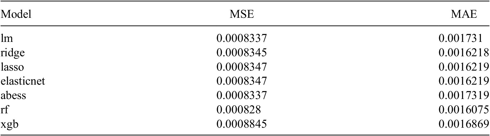
Table 1 reports mean squared error (MSE) and mean absolute error (MAE) for all models tested. The random forest (RF) model has the lowest MSE (
$ 0.000828 $
 ) and MAE (
$ 0.0016075 $
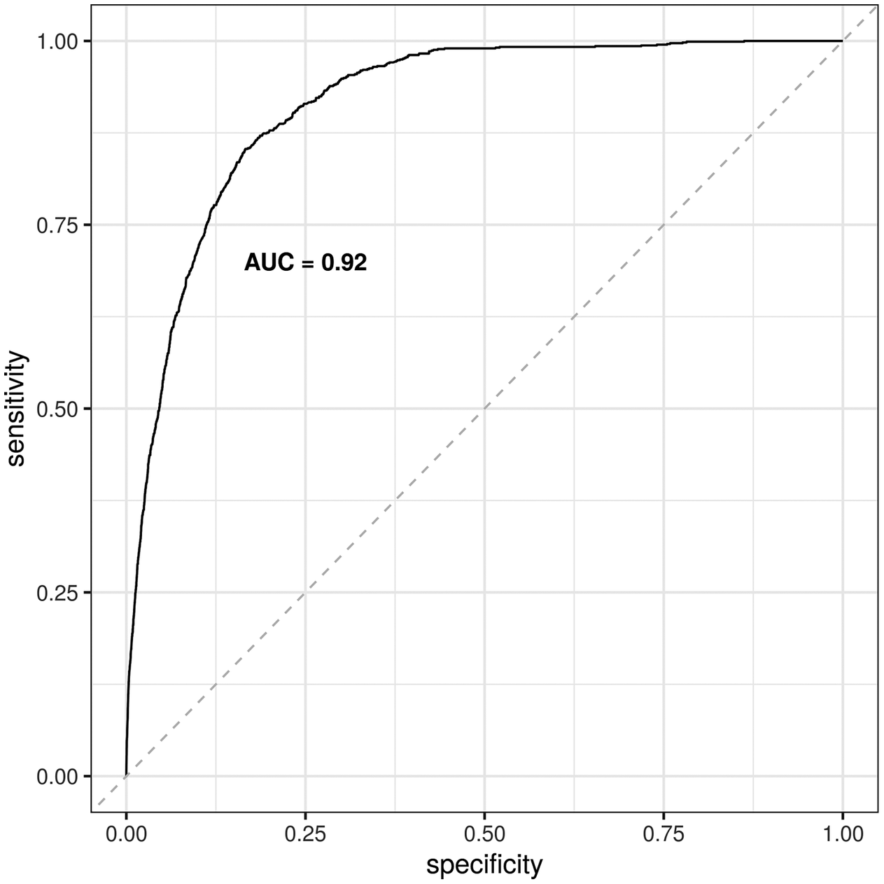
 ), so it outperforms all other options. The RF model also has an AUC of 0.92, shown in Figure 3, with a 95% CI of 0.908–0.922) (DeLong et al., Reference DeLong, DeLong and Clarke-Pearson1988; Robin et al., Reference Robin, Turck, Hainard, Tiberti, Lisacek, Sanchez and Müller2011). Based on this performance, the interpretation of results focuses on the RF model.
Summary of model performance

Table 1. Long description
The table consists of three columns: Model, M S E (Mean Squared Error), and M A E (Mean Absolute Error).
* l m: M S E 0.0008337, M A E 0.001731.
* ridge: M S E 0.0008345, M A E 0.0016218.
* lasso: M S E 0.0008347, M A E 0.0016219.
* elasticnet: M S E 0.0008347, M A E 0.0016219.
* abess: M S E 0.0008337, M A E 0.0017319.
* r f: M S E 0.000828, M A E 0.0016075.
* x g b: M S E 0.0008845, M A E 0.0016869.
The r f model shows the lowest M S E and M A E values among all listed models.
Note: Models were evaluated based on two measures of predictive accuracy: MSE (mean squared error) and MAE (mean absolute error). Included models are: lm (basic linear model, ordinary least squares), ridge regression, lasso regression, elasticnet regression, abess (adaptive best-subset selection), rf (random forest), and xgb (extreme gradient boosting).
ROC-AUC curve for random forest (RF) model, showing an AUC of 0.92.

4. Results and discussion
Figure 4 reports two variable importance plots from the random forest model. In both plots, the variables toward the top are the more important predictors. The plot on the left ranks predictors according to the proportion by which MSE increases if the predictor is left out (%IncMSE), and the plot on the right ranks predictors according to the increase in node purity (IncNodePurity). Changes in vegetation rank highly in both plots. In the first plot, the 5-year change in vegetation is the top feature and the 10-year change is the fourth feature; in the second plot, 10-year change and 5-year change in vegetation are the top two predictors. After that, there is a range of socioeconomic, demographic, public safety, and political features. In the first graph, employment rate, single-parent households, the homicide rate in 2009, prevalence of young men, abstention from voting, margin of victory, and the human development index are all in the top 10 predictors. In the second graph, Bolsa Familia (the financial assistance program for low-income families), the homicide rate in 2007, the prevalence of young men, effective number of candidates (ENC), abstention, employment rate, and the 5-year change in homicide rate are in the top 10. There is substantial overlap across the two plots, with the two measures of vegetation change, employment rate, prevalence of young men, abstention, and measures of violence appearing in the top 10 on both.
Variable importance plots based on the percent increase in MSE (%IncMSE) and increase in node purity (IncNodePurity). Variables included are: 5-year change in vegetation index (veg_change_5yr), 10-year change in vegetation index (veg_change_10yr), population density (pop_density), prevalence of young men (pop_young_male), homicide rate in various years from 2006 to 2010 (e.g., homicide_rate_2006), employment rate (employment_rate), proportion of single-parent households (single_parents), prevalence of the Bolsa Familia poverty-reduction program (Bolsa_Familia), economic inequality (inequality), human development index (human_development), margin of victory in last mayoral election (margin_of_victory), effective number of candidates from last mayoral election (ENC), partisan alignment of mayor and governor (alignment), abstention rate (abstention), and identifiers for the three major political parties of local mayors (PMDB, PSDB, and PT).

Figure 4. Long description
The figure consists of two vertical dot plots.
Left Panel: The x-axis is labeled percent Inc M S E and ranges from 1 to 7. The variables are ranked from highest to lowest importance as follows: veg underscore change underscore 5yr (highest, near 7), employment underscore rate, single underscore parents, veg underscore change underscore 10yr, homicide underscore rate underscore 2009, pop underscore young underscore men, abstention, margin underscore of underscore victory, human underscore development, alignment, inequality, homicide underscore rate underscore 2007, P M D B, pop underscore density, P S D B, homicide underscore rate underscore 2006, change underscore in underscore homicide underscore rate underscore 5yr, homicide underscore rate underscore 2010, E N C, Bolsa underscore Familia, P T, and homicide underscore rate underscore 2008 (lowest, near 1).
Right Panel: The x-axis is labeled Inc Node Purity and ranges from 0 to 4. The variables are ranked from highest to lowest importance as follows: veg underscore change underscore 10yr (highest, near 4.5), veg underscore change underscore 5yr, Bolsa underscore Familia, homicide underscore rate underscore 2007, pop underscore young underscore men, E N C, abstention, employment underscore rate, change underscore in underscore homicide underscore rate underscore 5yr, homicide underscore rate underscore 2010, human underscore development, homicide underscore rate underscore 2006, margin underscore of underscore victory, pop underscore density, homicide underscore rate underscore 2009, homicide underscore rate underscore 2008, inequality, single underscore parents, P S D B, alignment, P T, and P M D B (lowest, near 0).
Figure 5 complements the previous plots, reporting the distribution of minimal depth among the trees. Again, variables toward the top are most important. Minimal depth is the “depth of the node which splits on that variable and is the closest to the root of the tree. If it is low, then a lot of observations are divided into groups on the basis of this variable” (Paluszynska et al., Reference Paluszynska, Biecek and Jiang2020). The label identifies the mean minimal depth for each variable across all trees, and the x-axis identifies the number of trees any one variable was used for splitting. The following features appear in the top half of the graph: prevalence of young men, abstention, employment rate, Bolsa Familia, and human development, along with several measures of violence—homicide rates for 2006, 2007, 2008, and 2010, as well as the 5-year change in homicide rate—and the 10-year change in vegetation.
Variable importance plot based on minimal depth and mean. Variables included are: 5-year change in vegetation index (veg_change_5yr), 10-year change in vegetation index (veg_change_10yr), population density (pop_density), prevalence of young men (pop_young_male), homicide rate in various years from 2006 to 2010 (e.g., homicide_rate_2006), employment rate (employment_rate), proportion of single-parent households (single_parents), prevalence of the Bolsa Familia poverty-reduction program (Bolsa_Familia), economic inequality (inequality), human development index (human_development), margin of victory in last mayoral election (margin_of_victory), effective number of candidates from last mayoral election (ENC), partisan alignment of mayor and governor (alignment), abstention rate (abstention), and identifiers for the three major political parties of local mayors (PMDB, PSDB, and PT).

Figure 5. Long description
A horizontal stacked bar chart titled Minimal Depth and Mean (rf, full, y=embargo). The Y-axis is labeled Variable and the X-axis is labeled Number of trees, ranging from 0 to 50.
Each bar represents a variable, with segments colored according to a legend for Minimal depth ranging from 0 (red) to 15 (pink), and N A (gray). Lower minimal depth values indicate higher variable importance. Numerical labels on each bar indicate the mean minimal depth.
From top to bottom, the variables and their mean minimal depths are:
* pop_young_male: 2.86
* abstention: 2.9
* change_in_homicide_rate_5yr: 2.9
* homicide_rate_2007: 2.96
* employment_rate: 2.98
* homicide_rate_2008: 3
* Bolsa_Familia: 3.04
* homicide_rate_2010: 3.06
* veg_change_10yr: 3.08
* homicide_rate_2006: 3.2
* human_development: 3.22
* E N C: 3.3
* single_parents: 3.34
* veg_change_5yr: 3.42
* inequality: 3.46
* pop_density: 3.62
* homicide_rate_2009: 3.7
* margin_of_victory: 3.76
* P M D B: 5.58
* alignment: 5.7
* P T: 5.96
* P S D B: 6.72
The top variables are dominated by warm colors (orange and yellow, representing depths 1 to 3) across the majority of the 50 trees. The bottom four variables (political parties and alignment) show a shift toward cool colors (green and blue, representing depths 5 to 10), indicating significantly lower importance.
The next three graphs examine feature importance based on a combination of different measures of importance, that is, multi-way importance. Figure 6 captures multi-way importance based on the three least-correlated measures of importance: number of nodes, MSE increase, and times a root. Figure 7 captures multi-way importance based on measures of tree structure: number of nodes, times a root, and mean minimal depth. And Figure 8 captures multi-way importance based on the three measures of accuracy: MSE increase, node purity increase, and p-value. In Figures 6–8, variables that rank highly across all three measures are labeled to help identify the most important ones, and also indicate which combinations of variables are most important.
Multi-way importance based on three measures of importance: number of nodes (no_of_nodes), MSE increase, and times a root. The top 10 most important features are labeled, including: 10-year change in vegetation index (veg_change_10yr), population density (pop_density), prevalence of young men (pop_young_men), homicide rate in 2008 and 2010 (homicide_rate_2008 and homicide_rate_2010), 5-year change in homicide rates (change_in_homicide_rate_5yr), employment rate (employment_rate), prevalence of the Bolsa Familia poverty-reduction program (Bolsa_Familia), human development index (human_development), effective number of candidates from last mayoral election (ENC), and the abstention rate (abstention). More than 10 features are identified if there is a tie.

Figure 6. long description
The horizontal X-axis represents no_of_nodes ranging from 0 to 6000. The vertical Y-axis represents mse_increase ranging from 0e+00 to 1e-04. A legend on the right indicates that blue circles are top variables and black circles are non-top. The size of the circles corresponds to times_a_root from 0 to 5.
Data points are distributed as follows:
* At the top of the Y-axis near 3000 on the X-axis is a large blue bubble labeled homicide_rate_2008.
* Clustered between 3000 and 4000 on the X-axis and 0e+00 to 5e-05 on the Y-axis are several blue bubbles labeled from top to bottom: Bolsa_Familia, change_in_homicide_rate_5yr, homicide_rate_2010, E N C, abstention, pop_density, human_development, and employment_rate.
* To the far right near 6000 on the X-axis and 0e+00 on the Y-axis is a blue bubble labeled veg_change_10yr.
* At the bottom center near 4000 on the X-axis is a blue bubble labeled pop_young_men.
* Several smaller black non-top bubbles are scattered near the origin and along the bottom of the chart.
Multi-way importance based on measures related to the structure of trees: number of nodes (no_of_nodes), times a root, and mean minimal depth (mean_min_depth). The top 10 most important features are labeled, including: 5-year change in vegetation index (veg_change_5yr), 10-year change in vegetation index (veg_change_10yr), prevalence of young men (pop_young_male), homicide rate in 2008 and 2010 (homicide_rate_2008 and homicide_rate_2010), 5-year change in homicide rates (change_in_homicide_rate_5yr), employment rate (employment_rate), prevalence of the Bolsa Familia poverty-reduction program (Bolsa_Familia), human development index (human_development), effective number of candidates from last mayoral election (ENC), and abstention rate (abstention). More than 10 features are identified if there is a tie.

Figure 7. Long description
A scatter plot titled Multi-way importance r f, full, y equals embargo. The horizontal X-axis is labeled no_of_nodes ranging from 0 to 6000. The vertical Y-axis is labeled times_a_root ranging from 0 to 5. Data points are represented by circles where the size indicates mean_min_depth, with larger circles representing smaller values (3) and smaller circles representing larger values (6). Blue circles represent top variables, while black circles represent non-top variables.
* At the top of the Y-axis (value 5), three blue dots are clustered around X equals 3000, labeled homicide_rate_2008, E N C, and change_in_homicide_rate_5yr.
* At Y equals 4, two blue dots are clustered around X equals 3000, labeled abstention, homicide_rate_2010, and human_development.
* At Y equals 3, one blue dot and one black dot are near X equals 3000. The blue dot is labeled pop_young_men.
* At Y equals 2, a cluster of blue dots appears at X equals 3000, labeled employment_rate and Bolsa_Familia. Further right at X equals 6500, two blue dots are labeled veg_change_10yr and veg_change_5yr. A single black dot sits at X equals 1000.
* At Y equals 1, two black dots are located near X equals 3000 and one at X equals 1000.
* At Y equals 0, the largest black dot is at X equals 3500, with smaller black dots at X equals 1000 and near 0.
Multi-way importance based on measures related to predictive accuracy: MSE increase, node purity increase, and p-value. The top 10 most important features are labeled, including: 5-year change in vegetation index (veg_change_5yr), 10-year change in vegetation index (veg_change_10yr), prevalence of young men (pop_young_male), homicide rate in 2007 to 2010 (homicide_rate_2007 and homicide_rate_2010), 5-year change in homicide rate (change_in_homicide_rate_5yr), employment rate (employment_rate), prevalence of the Bolsa Familia poverty-reduction program (Bolsa_Familia), effective number of candidates from last mayoral election (ENC), and abstention rate (abstention). More than 10 features are identified if there is a tie.

Figure 8. Long description
The X-axis represents mse_increase ranging from 0e+00 to 1e-04. The Y-axis represents node_purity_increase ranging from 0 to 5. A legend on the right indicates p_value by color: red for less than 0.01, green for 0.01 to 0.05, and blue for greater than or equal to 0.1. Points with a thick black border are labeled as top variables.
* In the top-left corner, two red points with black borders show the highest node purity increase: veg_change_10yr and veg_change_5yr, both near 4.8 on the Y-axis and close to 0 on the X-axis.
* In the center-left region, a cluster of labeled points includes pop_young_men, Bolsa_Familia, homicide_rate_2007, abstention, E N C, change_in_homicide_rate_5yr, employment_rate, and homicide_rate_2010. These range between 1.8 and 3.0 on the Y-axis.
* Bolsa_Familia is the furthest right among the top-labeled variables, positioned near 5e-05 on the X-axis.
* Several unlabeled blue and red points are concentrated in the bottom-left quadrant, indicating lower importance across both measures.
* A single blue outlier is located at the far right of the plot, near 1.3e-04 on the X-axis and 1.5 on the Y-axis.
The features identified as most important across all three multi-way plots include: homicide rate in 2010, 5-year change in homicide rate, 10-year change in vegetation, Bolsa Familia, prevalence of young men, employment rate, ENC, and abstention. The 5-year change in vegetation, human development, and the homicide rate in 2008 also appear in two of the graphs. Measures that appear only in one graph are population density (Figure 6) and the homicide rate in 2007 (Figure 8).
One of the strengths of RF models like the one here is that they capture nonlinearities and interactions. There are 242 interactions in the model, and Figure 9 reports the 30 most frequent interactions. Table 2 complements the figure by showing these interactions in greater detail. In Figure 9, the x-axis identifies pairs of variables. The interactions are sorted in descending order of frequency, so the most frequent interactive pair is on the far left (and at the top of Table 2). The y-axis identifies the depth of each interaction. The top interactions involve the same variables highlighted earlier: homicide rates in several years, change in homicide rates, change in vegetation (5-year and 10-year), population density, the prevalence of young men, employment rate, Bolsa Familia, effective number of candidates (ENC), and abstention.
Depth of the 30 most frequent interactions, relevant trees only. Interactions appear left to right in descending order according to the number of occurrences. Variables included are: 5-year change in vegetation index (veg_change_5yr), 10-year change in vegetation index (veg_change_10yr), population density (pop_density), prevalence of young men (pop_young_male), homicide rate in each year from 2006 to 2010 (e.g., homicide_rate_2006), 5-year change in homicide rate (change_in_homicide_rate_5yr), employment rate (employment_rate), prevalence of the Bolsa Familia poverty-reduction program (Bolsa_Familia), effective number of candidates from last mayoral election (ENC), and the abstention rate (abstention).

Figure 9. Long description
A bar chart with the y-axis labeled mean underscore min underscore depth ranging from 0 to 3 and the x-axis labeled interaction. The chart displays 30 vertical bars representing variable pairs.
* Legend and Scales: A red horizontal line across the chart at approximately 1.75 represents the minimum. Black dots above the bars represent unconditional values. A color gradient scale for occurrences ranges from dark blue (41) to light blue (46).
* Data Trends: Bars are ordered from left to right by descending number of occurrences. The first bar on the left, pop underscore young underscore men colon veg underscore change underscore 10yr, is light blue (highest occurrences) with a mean depth of approximately 2.1. As the bars move right, the color shifts to dark blue, indicating fewer occurrences.
* Key Interactions: The interaction with the highest mean depth is homicide underscore rate underscore 2010 colon homicide underscore rate underscore 2007, reaching nearly 3.7. The interaction with the lowest mean depth shown is abstention colon abstention at approximately 1.8.
* Variable Pairs: Interactions include combinations of veg underscore change underscore 5yr, veg underscore change underscore 10yr, pop underscore density, pop underscore young underscore male, homicide underscore rate from various years, employment underscore rate, Bolsa underscore Familia, E N C, and abstention.
Variables involved in the 30 most frequent interactions, with mean minimal depth and frequency
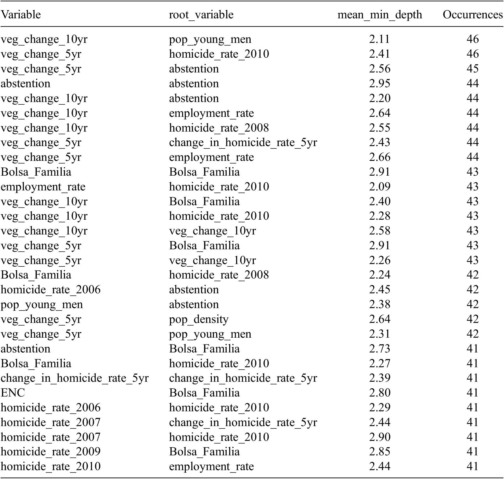
Table 2. Long description
The table contains four columns: Variable, root_variable, mean_min_depth, and Occurrences.
Top interactions by frequency include:
* veg_change_10yr and pop_young_men: mean_min_depth 2.11, 46 occurrences.
* veg_change_5yr and homicide_rate_2010: mean_min_depth 2.41, 46 occurrences.
* veg_change_5yr and abstention: mean_min_depth 2.56, 45 occurrences.
* abstention and abstention: mean_min_depth 2.95, 44 occurrences.
* veg_change_10yr and abstention: mean_min_depth 2.20, 44 occurrences.
* veg_change_10yr and employment_rate: mean_min_depth 2.64, 44 occurrences.
* veg_change_10yr and homicide_rate_2008: mean_min_depth 2.55, 44 occurrences.
* veg_change_5yr and change_in_homicide_rate_5yr: mean_min_depth 2.43, 44 occurrences.
* veg_change_5yr and employment_rate: mean_min_depth 2.66, 44 occurrences.
* Bolsa_Familia and Bolsa_Familia: mean_min_depth 2.91, 43 occurrences.
* employment_rate and homicide_rate_2010: mean_min_depth 2.09, 43 occurrences.
* veg_change_10yr and Bolsa_Familia: mean_min_depth 2.40, 43 occurrences.
* veg_change_10yr and homicide_rate_2010: mean_min_depth 2.28, 43 occurrences.
* veg_change_10yr and veg_change_10yr: mean_min_depth 2.58, 43 occurrences.
* veg_change_5yr and Bolsa_Familia: mean_min_depth 2.91, 43 occurrences.
* veg_change_5yr and veg_change_10yr: mean_min_depth 2.26, 43 occurrences.
Other notable interactions with 41 to 42 occurrences involve variables such as homicide_rate_2006, pop_density, E N C, and homicide_rate_2009, often interacting with Bolsa_Familia or homicide_rate_2010.
Note: Interactions appear top-to-bottom in descending order of frequency. Variables included are: 5-year change in vegetation index (veg_change_5yr), 10-year change in vegetation index (veg_change_10yr), population density (pop_density), prevalence of young men (pop_young_male), homicide rate in each year from 2006 to 2010 (e.g., homicide_rate_2006), 5-year change in homicide rate (change_in_homicide_rate_5yr), employment rate (employment_rate), prevalence of the Bolsa Familia poverty-reduction program (Bolsa_Familia), effective number of candidates from last mayoral election (ENC), and the abstention rate (abstention).
Summing up thus far, the variables that consistently emerge as most important include those that capture changes in the natural environment (vegetation change), violence and changes in violence (homicide rate and change in the homicide rate), demographic factors (population density and prevalence of young men), socioeconomic factors (Bolsa Familia, employment rate, and human development), and political factors that capture participation and the competitiveness of local politics (abstention and ENC). Some of the features found to be important—on their own and in combination with others in the interactions above—might seem unsurprising to some audiences, while others may be more surprising and deserve more attention.
Among unsurprising features, violence and vegetation changes are typically linked to illegal deforestation. Recalling the opening sections, deforestation is often associated with areas of prior vegetation loss, and illegal deforestation often occurs at the boundaries of legal areas of land conversion, for example, at the edges of cattle ranches or soy farms (Skidmore et al., Reference Skidmore, Moffette, Rausch, Christie, Munger and Gibbs2021). Other studies have used the registry of rural areas (Cadastro de Areas Rurais, CAR) (Carvalho et al., Reference Carvalho, Mustin, Hilário, Vasconcelos, Eilers and Fearnside2019) and similar administrative data on land use to try to approximate where these peripheral, rural areas at the edges of large landholdings might be. Violence is also a common feature of these rural areas where there is conflict over land grabbing and dispossession, and where the state has a weak presence (O’Donnell, Reference O’Donnell2001; Carvalho et al., Reference Carvalho, Mustin, Hilário, Vasconcelos, Eilers and Fearnside2019). For these reasons, it is also unsurprising that population density is linked to illegal deforestation. In Brazil, studies of local areas, including indigenous areas, find that roads are related to deforestation by facilitating land-grabbing and environmental crimes (Ferrante et al., Reference Ferrante, Andrade and Fearnside2021; da Silva et al., Reference da Silva, de Andrade, dos Santos and de Melo2023b). This might be especially true of new or informal, unregulated roads, as well as other types of transportation networks (e.g., airstrips and waterways).
For these reasons, related work focuses on human–environment interactions, including how development goals can collide with environmental protection. For instance, building infrastructure (e.g., roads) can be beneficial for development, but infrastructure projects can also drive environmental degradation (Kaczan, Reference Kaczan2020).
Other features may be more surprising and are not typically included in environmental monitoring or off-site approaches to detecting environmental crimes, so they merit greater attention. Indeed, these demographic, socioeconomic, and political factors highlight the interdisciplinary resonance and implications of the findings. These more surprising features include: (1) demographic factors like the prevalence of young men; (2) socioeconomic factors like the level of human development, the employment rate, and the poverty-reduction program Bolsa Familia; and (3) political factors like local margin of victory, effective number of candidates (ENC), and abstention.
Many of these more surprising features are familiar to scholars in criminology, as well as sociologists and demographers who study crime and violence. Social disorganization theory (Shaw and McKay, Reference Shaw and McKay1942; Sampson and Groves, Reference Sampson and Groves1989) provides a lens from those disciplines through which to understand these features. According to early versions of this theory, residential instability, resource deprivation, and ethnic heterogeneity were markers of unstable or disorganized communities, and this community disorganization was associated with higher rates of crime and violence (Shaw and McKay, Reference Shaw and McKay1942). Later work fleshed out the role of related factors like unsupervised youth, low participation or engagement in civic organizations, weak or sparse friendships, and family disruption, linking these factors to low collective efficacy or social cohesion, or the absence of community resilience to violence (Sampson and Groves, Reference Sampson and Groves1989; Sampson et al., Reference Sampson, Raudenbush and Earls1997). Generally, there is substantial support for social disorganization theory over time and across comparative contexts (Sampson and Groves, Reference Sampson and Groves1989; Sampson and Wilson, Reference Sampson and Wilson2012; Bellair, Reference Bellair2017).
Social disorganization theory helps to understand the importance of the prevalence of young men, employment rates, human development, and Bolsa Familia. The prevalence of young men is one of the structural aspects of population pressures associated with interpersonal violence, including homicides (Land et al, Reference Land, McCall and Cohen1990; Ingram and Marchesini da Costa, Reference Ingram and Marchesini da Costa2019a; Cullen et al., Reference Cullen, Peden, Francis, Cini, Azzopardi, Möller, Peden, Sawyer, Nathan, Joshi, Patton and Ivers2024). If violence is associated with illegal deforestation, and the prevalence of young men is associated with violence, it makes sense that the prevalence of young men would also be associated with illegal deforestation.
Considering that much illegal deforestation takes place at the peripheral boundaries of large cattle or soy farms, the kinds of labor required in these areas may attract young men. Alternatively, it may be supplied by criminal networks where young men are prevalent. In these remote, rural areas, the transient nature of this kind of labor mimics the residential instability, resource deprivation, and low supervision that are hallmarks of social disorganization accounts of crime and violence. Low or unstable employment rates also influence social disorganization and are correlated with crime (Land et al, Reference Land, McCall and Cohen1990; Baller et al., Reference Baller, Anselin, Messner, Deane and Hawkins2001). Another persistent finding in sociological and criminological studies is that adverse childhood experiences and exclusion—including maltreatment, family conflict, poverty, and low education—predict future gang involvement and entry into criminal networks (Carvalho and Soares, Reference Carvalho and Soares2016; Bauer et al., Reference Bauer, Martins, Hammerton, Gomes, Gonçalves, Menezes, Wehrmeister and Murray2024; Barker et al., Reference Barker, Bonell and Melendez-Torres2026). This also helps explain the association of human development (a composite measure of income, life expectancy, and education) with illegal deforestation, since low values of human development would tend to associate with poverty, mortality, illiteracy, and other adverse conditions, which resonate with social disorganization and are linked to crime (Baller et al., Reference Baller, Anselin, Messner, Deane and Hawkins2001). The poverty-reduction program Bolsa Familia would generally be expected to ameliorate these adverse conditions. However, it is also targeted at these conditions, so it may be identifying these markers of social disorganization, including resource deprivation, clarifying its importance. Though the prevalence of single-parent households is not among the top predictors in this study, the criminology literature also helps understand the relevance of this feature, since family disruption undermines social cohesion and can be an adverse childhood experience that contributes to social disorganization and reduced efficacy (Land et al, Reference Land, McCall and Cohen1990; Sampson et al., Reference Sampson, Raudenbush and Earls1997), and is a predictor of crime and violence (Ingram and Marchesini da Costa, Reference Ingram and Marchesini da Costa2019a).
Lastly, among the political features, margin of victory and the effective number of candidates measure the level of electoral competition and capture local political incentives. Where competition is low, a single party dominates local politics, which is often associated with traditional, patron-client exchanges where one or two families dominate politics, and which make it easier to establish networks of patronage or corruption, and generate few incentives to change (Beer, Reference Beer2006; Ríos-Figueroa, Reference Ríos-Figueroa2007; Ingram, Reference Ingram2013). Indeed, there is a literature in Brazil on local bosses or “colonels” (coroneis) (Leal, Reference Leal1977; Pinto Gil, Reference Gil2022) who wield substantial economic power and blur the lines between this private power and the public power of local government. Where a single political party is dominant, this private power and local government can become deeply enmeshed, and it would be easier to sidestep environmental controls. Conversely, where competition is higher, there is more turnover, traditional patronage networks tend to be disrupted, and politicians are generally more dynamic and responsive, including to environmental concerns. Regarding abstention, it is important to note that voting is mandatory in Brazil, so any abstention from voting is a strong signal of voter disengagement and lack of trust and confidence in the political process. In this regard, abstention is a signal of withdrawal from organizations and participation, a lack of efficacy, and a kind of anomie (Merton, Reference Merton1938) that fits within the social disorganization theory discussed above. Indeed, research on social capital in political science and the risks of declining participation in civic organizations (Putnam, Reference Putnam1993, Reference Putnam1995) resonates with the literature on social cohesion, collective efficacy, and community resilience and the connection of these community characteristics and crime (Ingram, Reference Ingram, Shirk, Wood and Olson2014) Thus, the competitiveness of local politics and abstention provide a bridge between political science and sociological approaches to crime and violence. Prior research establishes a relationship between these political factors and violence in Brazil (Ingram and Marchesini da Costa, Reference Ingram and Marchesini da Costa2019a), and this helps understand why these features are important predictors of illegal deforestation.
5. Conclusion
5.1. General summary
Detecting environmental crimes is important, especially in the Amazon biome. Existing approaches adopt either on-site or off-site approaches with various tradeoffs. Off-site approaches in Brazil tend to focus on the features of the physical environment derived from remote sensing, though a smaller set of approaches integrate administrative data from government registries of rural properties.
This study follows the off-site, machine-learning approach, includes features of the physical environment, and contributes to the advancement of environmental crime detection primarily in two ways: (1) leveraging a different kind of administrative data, namely embargoes—legal liens placed on properties for known environmental crimes—and (2) integrating a broad array of demographic, social, economic, political, and public safety measures as predictors. The embargo data identify known sites of environmental crimes, specifically illegal deforestation, and the analysis trains models to detect yet-unknown sites of illegal deforestation. The inclusion of the sociodemographic, economic, political, and public safety data expands environmental crime detection in a more interdisciplinary direction consistent with multicausal understandings of environmental crime.
5.2. Methods
The approach proceeded in three steps. First, using public administrative data on embargoes, we identified documented locations of illegal deforestation in the Legal Amazon. Second, we merged this information with data on a wide range of potential explanatory factors, including features of the physical environment from remote sensing, as well as demographic, socioeconomic, political, and public safety attributes at each location. Third, we divided the data into training and testing data, and trained a series of models. The random forest (RF) model performed best, and interpretation focused on this model.
5.3. Findings
Key findings show that the combination of violence, change in violence, vegetation change, population density, the proportion of the population that is young and male, human development, employment rate, effective number of parties (ENC), and abstention are predictive of illegal deforestation. Some of the findings are unsurprising, including the relevance of vegetation change and violence. However, other findings are more surprising, including those that show the predictive importance of socioeconomic and political features.
5.4. Practical implications
The practical implications of these findings relate primarily to (1) the value of interdisciplinary approaches to environmental crime detection, (2) collaborations with government, and (3) enhanced safety of environmental crime detection. The surprising importance of social, economic, and political variables highlights the value of interdisciplinary approaches in this field and supports multicausal or multifactorial approaches to illegal deforestation. The socioeconomic and political features in particular indicate that integrating a political-economy framework to environmental crime detection can yield valuable insights, and motivate future interdisciplinary work. The administrative data on embargoes were vital. It would be promising to coordinate with government agencies to see what other data are available, or to engage in a mutual feedback process to see how future analyses could be improved, or how administrative data collection and sharing could be improved. And the remote, off-site detection of environmental crimes has several benefits, including reducing costs and avoiding security risks, so the approach here—and improving it over time—helps build better and safer means of environmental crime detection.
5.5. Limitations
The analysis has some limitations, including the use of somewhat older demographic, socioeconomic, and political data from 2000 to 2011. These data were used because a wide range of predictors were well-organized across 10 years during this time frame. The vegetation data from older satellite imagery also have reduced spatial resolution. Further, computational complexity limited some aspects of the analysis, including interpretation of a proximity matrix.
5.6. Future prospects
Future research can address the limitations noted above. A natural next step is to update and expand the data. The quality and availability of data are increasing in Brazil, especially with satellite imagery with better spatial resolution since 2018. Other projects that systematize geo-spatial data of higher quality can also be leveraged in the future. Further, Brazil’s federal government is more supportive of environmental protection since 2022, which should make administrative data like that used here more accessible and transparent. Future work can employ the approach here with these more recent data, and access to a high-performance computing cluster can solve some of the computational challenges. Interdisciplinary collaboration is also promising, including combining efforts with both (a) researchers from other fields and (b) government. Doing so promises improved results and additional insights, and would strengthen forest enforcement. The approach can also be extended to other illicit behavior, in Brazil and elsewhere.
Data availability statement
Replication materials are available at Harvard Dataverse: https://doi.org/10.7910/DVN/723MZQ.
Acknowledgments
Earlier versions of the methods in this article were presented in 2024 at the University of California, Irvine, and in 2025 at the annual meeting of the New England Political Science Association (NEPSA), and at Conference on Applied Research Methods and Data Collection with Hard-to-Reach (H2R) and Hidden Populations, Nuffield College, Oxford University. I am grateful to all participants for their comments. I am also especially grateful to Bruce Desmarais for his instruction and continued correspondence on methods. All errors are my own.
Author contribution
The author made the following contributions. Conceptualization: M.I. Funding acquisition: M.I. Data curation: M.I. Formal analysis: M.I. Supervision: M.I. Validation: M.I. Methodology: M.I. Project administration: M.I. Resources: M.I. Software: M.I. Investigation: M.I. Writing—original draft preparation: M.I. Writing—review and editing: M.I. Visualization: M.I. Final approval: M.I.
Funding statement
The methods for this project were developed in part with funding from the Faculty Resource Allocation Program (FRAP-A) at the University at Albany, award no. 97969.
Competing interests
The authors declare none.
Ethics statement
The research meets all ethical guidelines, including adherence to the legal requirements of the study country.





 Open access

