


1. Introduction
Stomata are pores found on the surface of plant leaves that perform critical roles in gas exchange and transpiration (Cowan & Troughton, Reference Cowan and Troughton1971; Willmer & Fricker, Reference Willmer and Fricker1996). Generally, these structures are found on the leaf epidermis but can also be present on stems. Certain phenotypes related to stomata, such as stomatal density (number of stomata per unit area) and stomatal distribution, can adapt according to environmental variations (Hetherington & Woodward, Reference Hetherington and Woodward2003), including fluctuations in
$\text {CO}_2$
 concentration, humidity and light exposure (Cai & Cao, Reference Cai and Cao2004), driving adaptations in photosynthetic capacity across different climates. This results in significant plasticity in the leaf epidermis, including changes in stomatal density.
Stomatal size and density vary between species and environmental conditions, ranging from 10 to 80
$\mu $
 m in length, while stomatal density can range from 5 to 1,000 per mm
$\!\!^{2}$
 of epidermis (Eckerson, Reference Eckerson1908). Gas exchange simulations show an inverse correlation between stomatal size and density, indicating a compensatory relationship between
$\text {CO}_2$
 uptake and water transpiration (Beerling & Woodward, Reference Beerling and Woodward1997). Additionally, light intensity and quality are critical for stomata plasticity, influencing the plant’s ability to adapt the photosynthetic capacity to different lighting conditions (Murchie & Horton, Reference Murchie and Horton1997).
Since stomatal distribution phenotypes exhibit high plasticity, novel approaches are required to identify intrinsic characteristics based on environmental fluctuations. Despite the use of geometric morphometry in taxonomic classification and phenotypic plasticity analysis (Viscosi & Cardini, Reference Viscosi and Cardini2011), there is a lack of methods to characterize stomatal distribution as a parameter for quantifying plant adaptation. While other computational approaches have modelled stomata through cellular nonlinear networks to simulate analogue computation (Peak et al., Reference Peak, Hogan and Mott2023) or via non-steady-state dynamical equations to predict conductance under fluctuating conditions (Liu et al., Reference Liu, Wang, Magney and Frankenberg2024), these typically focus on physiological flux rather than spatial pattern recognition. Some works propose to evaluate stomatal distribution over the surface of purple abaxial epidermis in extant plants using interstomatic distances as a parameter; however, they do not measure the extent of adaptation under induced environmental changes (de Almeida Filho, Reference de Almeida Filho2018).
The geometry of stomatal distribution on leaf surfaces can provide quantitative parameters that quantify how environmental changes affect plants. Plants exhibit phenotypic plasticity by adjusting stomatal spatial distribution as a survival strategy against environmental stressors, which we approach from a network perspective. In this context, stomata represent vertices and their spatial relationships represent edges. Unlike studies aimed at species identification (da Silva et al., Reference da Silva, Oliveira, Filho, Pinheiro, Rossatto, Kolb and Bruno2016), the goal here is to explore a pattern recognition method capable of separating environmental conditions where plasticity is fundamental.
Proposed workflow to use LLNA as a pattern recognition method.

Figure 1. Long description
The flowchart is organized into four numbered sections.
1. Network Construction: This section begins with 1.1 Stomatal image, showing a microscopic view of plant tissue. An arrow points to 1.2 Centroids, which displays a scatter plot of points. A zoomed-in red dashed box labeled Euclidean distance shows points with overlapping circular radii of 100 micrometers. This leads to an Adjacency matrix with binary values (0 and 1). Finally, 1.3 Network shows a graph of nodes connected by lines.
Stomatal Dataset: The network expands into a collection of geometric shapes (circles, squares, and pentagons) in gray and blue. A subset is circled and labeled (*) Rule Selection.
2. L L N A: Below the dataset, three network graphs show nodes changing from white to black based on a threshold T sub l. Below these graphs is a matrix of binary code.
3. Feature extraction: An arrow from L L N A points to a column vector containing mu sub 1, mu sub 2, through mu sub N. This leads to a final box containing various mu vector notations including mu sub S, mu sub L, and mu sub w.
4. Classification: An upward arrow leads to the final stage where the geometric shapes from the dataset are grouped into three distinct clusters separated by curved lines. An arrow from the right labeled Baseline comparison points into this classification area.
Information of the dataset of networks studied

Table 1 Long description
The table is organized into six columns under two main headers: Stomata dataset and Data split.
Header Row 1:
- Stomata dataset covers columns 2 through 4.
- Data split covers columns 5 and 6.
Header Row 2:
- Column 1: Species name.
- Column 2: Number of classes or environmental conditions.
- Column 3: Specific classes or environmental conditions.
- Column 4: Number of images.
- Column 5: Number of networks for training or validation.
- Column 6: Number of networks for rule selection.
Data Rows:
1. Ctenanthe: 2 classes (L 4 h, L 24 h); 36 images; 36 training/validation networks; no rule selection networks.
2. Trandescantia: 3 classes (Environment, L 4 h, L 24 h); 18 images; 12 training/validation networks; 6 rule selection networks.
3. Callisia: 3 classes (Environment, C O sub 2 down arrow, C O sub 2 up arrow); 15 images; 15 training/validation networks; no rule selection networks.
Pattern recognition using complex networks has achieved success in various tasks (Costa et al., Reference Costa, Rodrigues, Travieso and Boas2007, Reference Costa, Oliveira, Travieso, Rodrigues, Villas Boas, Antiqueira, Viana and da Rocha2011; Miranda et al., Reference Miranda, Machicao and Bruno2018), where network properties serve as topological fingerprints for environmental conditions. Structural measurements, such as clustering coefficient, degree and average path length, are commonly employed to characterize topological properties and have demonstrated reasonable performance (Costa et al., Reference Costa, Rodrigues, Travieso and Boas2007). More recently, graph-based methods have emerged, such as deep topological embedding (DTE) (Scabini et al., Reference Scabini, Ribas, Ribeiro and Bruno2022), deterministic tourist walk-based (DTWB) (Merenda & Bruno, Reference Merenda and Bruno2023) and deep graph convolutional neural networks (DGCNNs) (Zhang et al., Reference Zhang, Cui, Neumann and Chen2018). However, alternative approaches, such as network automata, have shown interesting properties for complex tasks (Machicao et al., Reference Machicao, Corrêa, Miranda, Amancio and Bruno2018; Miranda et al., Reference Miranda, Machicao and Bruno2016;Ribas et al., Reference Ribas, Machicao and Bruno2020; Zielinski et al., Reference Zielinski, Ribas, Machicao and Bruno2024). By simulating emergent behaviours, these methods provide a dynamical perspective on network evolution that can offer complementary insights when identifying subtle environmental adaptations.
In this study, we utilize pre-identified stomatal centroids to construct graphs and apply the Life-Like Network Automata (LLNA) method (Miranda et al., Reference Miranda, Machicao and Bruno2016) to accurately classify environmental conditions to which three plant species were subjected: Ctenanthe oppenheimiana, Tradescantia zebrina and Callisia repens. We adopted this method due to the high performance achieved in other classification tasks, such as authorship attribution (Machicao et al., Reference Machicao, Corrêa, Miranda, Amancio and Bruno2018), and in various extended versions of the LLNA framework (Ribas et al., Reference Ribas, Machicao and Bruno2020; Zielinski et al., Reference Zielinski, Ribas, Machicao and Bruno2024).
2. Material and methods
2.1. Method workflow
An overview of the pattern recognition method is shown in Figure 1. First, we introduce the network model for constructing networks from stomatal imagery, including a data split that allocates a small portion for LLNA rule selection. Next, we apply the LLNA and its corresponding feature extraction. The metrics derived from the LLNA dynamics are then utilized to classify the environmental conditions of the stomata across various plant species. Finally, we compared these results with baseline methods.
2.2. Images dataset
We used the stomatal image dataset acquired from the Scientific Computing Group of the São Carlos Institute of Physics (IFSC) (Supplementary Material). A summary of the dataset is presented in Table 1.
This dataset contains leaf images obtained by optical microscopy from three plant species: Ctenanthe oppenheimiana, Tradescantia zebrina and Callisia repens. Each image includes corresponding segmented binary images, with the centroids of each stoma manually identified by a specialist. The plants were subjected to one of two different stress conditions: light exposure and injection of
$\text {CO}_2$
 , as detailed in Section 2.3.
2.3. Crop, acclimation and microscopy
-
• Ctenanthe oppenheimiana: Plants, measuring 5–8 cm, were planted in standard Carolina substrate (Carolina soil, Brazil). Samples were acclimated in a controlled growth chamber (Eletrolab EL212/4G-RS) with continuous $55\%$
 relative humidity, a photon flux of 100
$\mu $
mol
$/\mathrm { m}^{2}\times $
s and a temperature of 25
$^{\circ }$
C. Two light/dark photoperiods were tested: 24 h (L24) and 4 h (L4) per day for 60 days, resulting in 18 images per condition. Samples are shown in Figure 2a.Figure 2.
Stomatal network modelling. The first column shows microscopic images of leaf abaxial epidermis from species: (a) Ctenanthe oppenheimiana (4 h and 24 h photoperiods); (b) Tradescantia zebrina (natural environment and 4 h and 24 h photoperiods) and (c) Callisia repens (natural environment, bottled $\text {CO}_2$
flow and bottled control). Scale bars are provided to account for different magnifications (100
$\times $
for Ctenanthe; 15
$\times $
for others). Subsequent columns display the resulting networks across different threshold radii
$T_l$
(red circle). These thresholds are calibrated to each image scale to capture the topological transition from sparse to dense connectivity (vertices in green, edges in grey).Figure 2. Long description
The grid is organized into three main sections.
Section a, Ctenanthe oppenheimiana, contains two rows. The first row shows a 4 h photoperiod with a microscopic photo followed by four network graphs at thresholds of 100, 120, 140, and 160 micrometers. A red circle indicates the threshold radius R sub l. As the radius increases, the grey edges connecting green vertices become more dense. The second row shows a 24 h photoperiod with significantly higher vertex density and more complex connectivity across the same thresholds.
Section b, Tradescantia zebrina, contains three rows: natural, 4 h photoperiod, and 24 h photoperiod. The network graphs use thresholds of 300, 320, 340, and 360 micrometers. The vertex distribution is highly regular and dense compared to section a, with connectivity increasing horizontally as the threshold radius grows.
Section c, Calissia repens, contains three rows: natural, C O sub 2 gas injection with an upward arrow, and C O sub 2 control with a downward arrow. It uses the same 300 to 360 micrometer thresholds as section b. The C O sub 2 injection row shows the highest density of green vertices, appearing as a nearly solid mass of points, while the control row shows slightly more sparse distribution.
All graphs include X and Y axes ranging from 0 to 2500 for section a and 0 to 1000 for sections b and c. Scale bars are present in the top right of the final column for each species.
-
• Tradescantia zebrina: Plants were acclimated in the same controlled growth chamber under identical conditions for 68 days. A third group was maintained under uncontrolled conditions in an external environment. A total of six images were obtained for each condition. This collection was previously described by Florindo et al. (Reference Florindo, Landini, Almeida Filho and Bruno2015). Samples are shown in Figure 2b.
-
• Callisia repens: Three experimental groups were used. The first was sealed in a bottle with Carolina soil and subjected to a $\text {CO}_2$
gas stream (1,500 ppm for 6 h/day over 30 days). The second group was treated similarly but without the
$\text {CO}_2$
flow. In both bottled groups, relative humidity was maintained between 85% and 90% during the daily 6-h cycle. A third group was collected from a natural, uncontrolled environment in July 2015 (georeferenced at
$-$
22.007 S;
$-$
47.894 W). Five images were captured for each condition. Samples are shown in Figure 2c.


Regarding imaging specifications, images were captured at different magnifications depending on the species. For Ctenanthe oppenheimiana, a 100
$\times $
 objective lens was used, resulting in a pixel scale of 0.347
$\mu $
 m/px and a resolution of
$2,560\times 1,920$
 pixels. For Tradescantia zebrina and Callisia repens, images were captured at 15
$\times $
 magnification, corresponding to 4.65935
$\mu $
 m/px and
$1,388\times 1,038$
 pixels. These specific optical scales were used for all subsequent spatial measurements and pixel-to-micron conversions.
2.4. Stomatic network modelling
Figure 2 exemplifies the steps for the construction of the stomatal network model, as proposed by Backes et al. (Reference Backes, Casanova and Bruno2009) and Florindo et al. (Reference Florindo, Landini, Almeida Filho and Bruno2015). In this model, each stoma corresponds to a vertex in the lattice, and the rule for establishing the edges is based on the Euclidean distance between pairs of stomata governed by a threshold
$T_l$
 .
Each image contains a different number of stomata (vertices) positioned at the centres of circles; thus, the threshold
$T_l$
 defines the radius of connectivity of a stoma with its nearest neighbours. A distance matrix containing all distances between stomata pairs in each image is obtained through the Euclidean distances between each pair of vertices (
$W$
 ). This matrix is then transformed into several networks represented by the adjacency matrix
$A_{T_{l}}$
 depending on the threshold
$T_l$
 , as given by Equation (1). Specifically, if the distance between a pair of stomata is less than or equal to the threshold, then an edge is established between them:

Since the characterization of these networks is carried out through a series of transformations in which
$T_l$
 is incremented between
$T_{ini}$
 and
$T_{Q}$
 (the initial and final values of the threshold), it allows for a multi-scale analysis of the topology (Backes et al., Reference Backes, Casanova and Bruno2009). Since the centroid coordinates are provided in the real scale of the plant, the pixel-based image coordinates are converted using a specific scale factor for each species (as detailed in Section 2.3). For instance, in Ctenanthe oppenheimiana, a factor of 0.347
$\mu $
 m/px was applied. From top to bottom, Figure 2 presents samples of abaxial epidermis images of each species of plant and the corresponding environmental condition.
Figure 2a illustrates the network construction process following Equation (1). On the left side of the figure, the microscopic image of a leaf of Ctenanthe oppenheimiana is shown. The red circles represent the centroids of the stomata identified in the segmented binary image. On the right side, four resulting networks are presented, each corresponding to a specific radius threshold
$T_{l}$
 . For illustration, various thresholds
$T_{l}$
 are shown to demonstrate the topological evolution. Note that as
$T_{l}$
 increases, more connections are established between stomata centroids (nodes), leading to higher network connectivity.
Considering that different networks can be obtained, the threshold
$T_l$
 must be limited according to the size of the image. Note that in the networks of the species Tradescantia zebrina and Callisia repens, the thresholds are numerically higher because the image samples have lower magnification (15
$\times $
 vs. 100
$\times $
 ), which results in a different spatial distribution of centroids within the field of view.
In Figures 2a and b, it can be observed that the epidermis of plants exposed to a 24-h daily photoperiod has a higher stomata density than plants exposed to 4 h. Due to this fact, networks constructed based on threshold distances (
$T_l$
 ) become highly connected in images where the stomatal density is larger. Due to the high plasticity of the plant, the number of stomata (vertices) of plants exposed to 24-h daily illumination is proportionally higher than in plants exposed to 4 h for the same threshold range. Likewise, in Figure 2c, which corresponds to the species Callisia repens, it is observed that higher
$\text {CO}_2$
 injection correlates with an increase in stomatal density and therefore leads to higher network connectivity for the same threshold values.
2.5. Life-like network automata
The LLNA
$\mathcal {R}$
 can be defined by the tuple
$\mathcal {R} = \langle \mathcal {T},\mathbf {S}, s_{0},\phi \rangle $
 (Miranda et al., Reference Miranda, Machicao and Bruno2016). The tessellation
$\mathcal {T}$
 represents the network topology, where each vertex is represented by a cell
$v_i$
 connected to its
$k_i$
 neighbours.
$\mathbf {S}$
 is the set of binary states, where
$s_i = 1$
 (live) and
$s_i = 0$
 (dead). The
$s(c_i,t)$
 function indicates the state of the cell
$c_i$
 at time
$t$
 ; thus,
$s_0$
 represents the initial configuration of all cells and
$\phi $
 is the transition function, that is, the rule governing the dynamics of the network automata, which defines how the cell states are updated.
The LLNA transition function (
$\phi $
 ) is defined as

where the neighbourhood density
$\rho _i$
 of node
$i$
 is defined as the proportion of active neighbours, that is:

where
$A_{ij}$
 is the adjacency matrix of the network and
$k_i$
 is the number of neighbours (degree) of node
$i$
 .
In Equation (2), the variables
$x$
 and
$y$
 represent the conditions of the Life-Like rule expressed in the form B
$x_0x_1\ldots x_8$
 -S
$y_0y_1\ldots y_8$
 , where B and S represent the ‘born’ and ‘survive’ conditions, respectively, and
$x_i, y_i \in \{0, \dots , 8\}$
 . The LLNA establishes a correspondence between the transition function and the rules of the two-dimensional Life-Like CA family (Bx-Sy). While the Moore neighbourhood traditionally uses eight fixed neighbours (
$r=9$
 ), the LLNA generalizes this to graphs using the neighbourhood density (Equation (3)), defined as the proportion of active neighbours. This ensures that the transition rules remain consistent regardless of the varying number of neighbours in the network. Therefore, there are a total of
$2^{18} = 262,144$
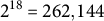 transition rules available to find optimal solutions for a particular problem (Miranda et al., Reference Miranda, Machicao and Bruno2016).
2.6. Feature extraction
Using a given rule, the dynamics of a network automaton produce a time-evolution pattern (TEP) that represents the state sequence over time for each node. Each node can be analysed as a sequence of zeros and ones. From a TEP, various measurements can quantify individual node properties, allowing for network characterization. For feature extraction, we selected the suggested metrics: Shannon entropy (
$\mu _S$
 ), word length (
$\mu _W$
 ) and Lempel–Ziv complexity (
$\mu _L$
 ). Since these LLNA metrics use the number of bins
$b$
 as a parameter, we used the same ones as suggested by Miranda et al. (Reference Miranda, Machicao and Bruno2016).
The first feature vector,
$\mu _S$
 , represents the distribution of Shannon entropy values ranging from 0 to 1. We calculated the Shannon entropy for each node and generated a histogram by dividing the interval
$[0,1]$
 into
$b=20$
 bins, resulting in 20 descriptors reflecting their frequencies. The second feature vector (
$\mu _W$
 ) captures the distribution of word lengths, defined as a sequence of ones surrounded by zeros. For instance, in
$q=(00\textbf {1111}0\textbf {111}000)$
 , there is one word of length four and another of length three. The maximum word length is limited by the number of evolution steps; since words longer than 40 occur infrequently, we considered only shorter words. The histogram bins have a length of 2, yielding 20 descriptors for
$\mu _W$
 . The final feature vector (
$\mu _L$
 ) consists of the Lempel–Ziv complexity distribution, also divided into
$b=20$
 bins and normalized by the maximum value across the samples. Additionally, we created a composite vector by concatenating the three metrics
$[\vec {\mu }_S, \vec {\mu }_W, \vec {\mu }_L]$
 , as well as the average values for these measures:
$[\langle \mu _S\rangle , \langle \mu _W\rangle , \langle \mu _L\rangle ]$
 .
2.7. Baseline methods
To characterize the topological properties of the stomatal networks and establish a robust comparative framework, we employed two sets of evaluation approaches. First, we calculated a set of traditional network measurements (Costa et al., Reference Costa, Oliveira, Travieso, Rodrigues, Villas Boas, Antiqueira, Viana and da Rocha2011), including: average degree (
$\langle k\rangle $
 ), which reflects overall connectivity; average hierarchical degrees at levels 1 (
$\langle H_{k_1}\rangle $
 ) and 2 (
$\langle H_{k_2}\rangle $
 ), indicating immediate and neighbourhood connectivity; average clustering coefficient (
$\langle cc\rangle $
 ), quantifying node grouping; average path length (
$\langle l \rangle $
 ), providing insight into information flow efficiency; and the degree Pearson correlation (
$\rho _P$
 ), to identify assortative mixing patterns.
In addition to these structural metrics, we compared our LLNA approach against three selected graph-based classification methods to capture a broader spectrum of computational paradigms. The DTE method (Scabini et al., Reference Scabini, Ribas, Ribeiro and Bruno2022) transforms network topology into high-dimensional tensor representations via tensor decomposition for classification. The DTWB approach (Merenda & Bruno, Reference Merenda and Bruno2023) generates discriminative features by simulating deterministic walker movements to create histograms of trajectory lengths. Finally, the DGCNN (Zhang et al., Reference Zhang, Cui, Neumann and Chen2018) utilizes hierarchical graph convolutions and TopK pooling to learn multi-scale graph representations for classification through fully connected layers. These specific methods were chosen because they operate effectively on unweighted whole-graph structures without requiring rich node or edge attribute matrices, which are absent in our network dataset. This constraint makes heavily parameterized or feature-dependent alternatives, such as standard graph transformers or dense graph neural networks (GNNs), less suitable for this specific task. By incorporating tensor decomposition, deterministic walks and deep learning, this selection provides a diverse, though non-exhaustive, framework to evaluate our approach.
2.8. Rule selection
To identify candidate rules capable of distinguishing environmental stressors, we adopted a generalization protocol using a subset of Tradescantia zebrina. As shown in Table 1, only two images per class were used for rule selection, while the remaining images and the other two species (Ctenanthe and Callisia) were reserved to evaluate the classifiers’ performance. This protocol was designed to verify if the LLNA captures universal topological signatures of stomatal distribution that remain consistent across different species and stress types, without requiring re-optimization for each species.
We exhaustively evaluated each of the 262,144 rules of the Life-Like family in the set of stomata networks for rule selection. The networks were obtained using a threshold of
$T_l= 512\, \mu $
 m (equivalent to 110 pixels). To characterize the LLNA dynamics, a feature vector was created by concatenating the Shannon entropy and the Lempel–Ziv
$[\vec {\mu }_S, \vec {\mu }_L]$
 distributions into 40 descriptors (Miranda et al., Reference Miranda, Machicao and Bruno2016). Both distributions were windowed into
$b=20$
 bins and submitted to the k-nearest neighbours (kNN) classifier.
2.9. Classification task
We used the LLNA approach to extract intrinsic patterns from stomata networks aiming to distinguish between environmental conditions, aiding our understanding of plasticity. In the training phase, this technique extracts feature patterns for each stomata network (condition), which are then used to classify unseen instances during the classification phase.
After obtaining the feature vectors, we applied the kNN (for rule selection only) and support vector machine (SVM) algorithms, comparing our results with baseline methods. The SVM classification was performed using the sequential minimal optimization (SMO) algorithm with a polynomial kernel (exponent
$E=1.0$
 ) and a complexity parameter
$C=1.0$
 in Weka software (version 3.8), employing default settings to ensure a standardized comparison.
We conducted one experiment for each plant species, employing a
$k$
 -fold cross-validation strategy (Bishop, Reference Bishop2006) to assess classification performance. To maximize the use of our dataset while ensuring statistical robustness, we set
$k=10$
 for Ctenanthe and Tradescantia, and
$k=5$
 for Callisia due to its sample size. The entire process was repeated across
$100$
 independent experiments. This method splits the data into two sets: a training dataset for model training and a test set for validation. As these sets are mutually exclusive, the cross-validation method provides a reliable evaluation strategy. This procedure ensures that every sample is used for both training and testing in independent folds.
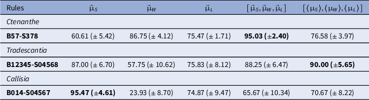
Classification accuracy rates (%) and standard deviations for LLNA-based feature extraction
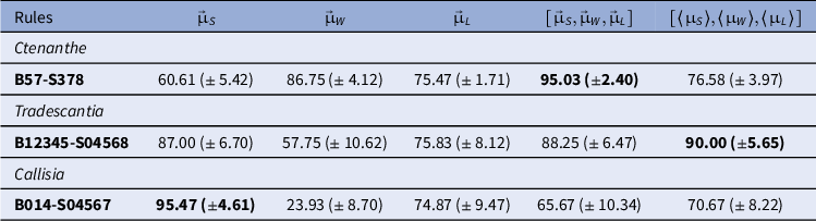
Table 2 Long description
The table consists of six columns and six data rows.
Column headers from left to right are:
1. Rules
2. mu vector sub S
3. mu vector sub W
4. mu vector sub L
5. open bracket mu vector sub S, mu vector sub W, mu vector sub L close bracket
6. open bracket average mu sub S, average mu sub W, average mu sub L close bracket
Data rows by species:
- Ctenanthe (B 5 7 minus S 3 7 8): 60.61 plus or minus 5.42; 86.75 plus or minus 4.12; 75.47 plus or minus 1.71; 95.03 plus or minus 2.40 (bold); 76.58 plus or minus 3.97.
- Tradescantia (B 1 2 3 4 5 minus S 0 4 5 6 8): 87.00 plus or minus 6.70; 57.75 plus or minus 10.62; 75.83 plus or minus 8.12; 88.25 plus or minus 6.47; 90.00 plus or minus 5.65 (bold).
- Callisia (B 0 1 4 minus S 0 4 5 6 7): 95.47 plus or minus 4.61 (bold); 23.93 plus or minus 8.70; 74.87 plus or minus 9.47; 65.67 plus or minus 10.34; 70.67 plus or minus 8.22.
Note: Feature vector dimensions are scaled according to the number of thresholds: 140, 420 and 21 descriptors for Ctenanthe oppenheimiana, and 320, 960 and 48 for Tradescantia and Callisia, respectively.
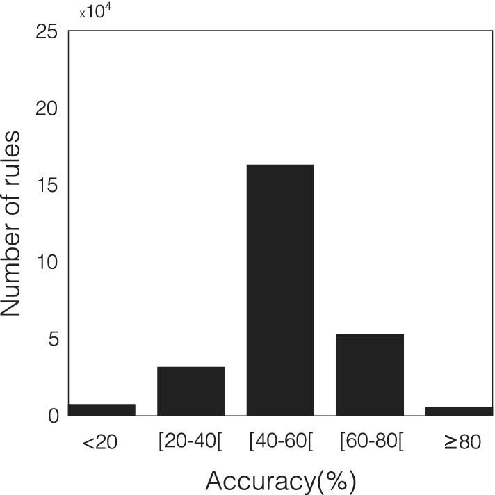
Histogram of the distribution of the 262,144 rules of the Life-Like family based on accuracy rates. The rule selection utilized stomata from the species Tradescantia zebrina. Shannon entropy and Lempel–Ziv complexity were considered only as feature vectors for the kNN classifier.

We further analysed the results using confusion matrices, which detail the relationship between predicted and real classes for each distinct environmental condition. A confusion matrix identifies performance patterns:
$\alpha _{m_i,m_i}$
 indicates instances correctly assigned to class
$m_i$
 , while
$\alpha _{m_i,m_j}$
 shows instances of class
$m_i$
 incorrectly assigned to class
$m_j$
 . This information is particularly useful for identifying samples that the proposed technique struggles to discriminate.
3. Results
The LLNA method was employed to characterize the phenotypic plasticity of the species Tradescantia zebrina, Callisia repens and Ctenanthe oppenheimiana when subjected to stress conditions. The dataset of networks used for validation is detailed in Table 1.
3.1. Configurations
3.1.1. Network threshold calibration.The distance threshold (
$T_l$
 ) range for network construction was tailored for each species to compensate for variations in optical magnification and stomatal density. For Ctenanthe oppenheimiana, we used seven thresholds ranging from
$T_{ini}=140$
 to
$T_{Q}=260\, \mu $
 m. For Tradescantia zebrina and Callisia repens, the feature vector was expanded to
$16$
 thresholds from
$T_{ini}=400$
 to
$T_{Q}=640\, \mu $
 m. All pixel-to-micron conversions followed the optical scales defined in Section 2.3.
3.1.2. Life-like rules selection.Figure 3 shows the histogram distribution of the accuracy rates obtained for the rulespace of the Life-Like family. More than 5,000 rules achieved accuracy rates above 80%, confirming that several automata rules can effectively discriminate stomatal stress patterns. From this universe, we selected the 400 best-performing rules for the final classification stage. These candidate rules, originally identified using a subset of Tradescantia zebrina, were then used to train and test the models for all three species. This approach evaluates the generalization power of the rules across different plant species and environmental stressors.
3.2. Performance analysis
We adopted the strategy of concatenating descriptors obtained from the networks transformed by each value of
$\delta _{T_l}$
 , as proposed by Backes et al. (Reference Backes, Casanova and Bruno2009).
The feature vectors
$\vec {\mu }_S$
 ,
$\vec {\mu }_W$
 and
$\vec {\mu }_L$
 were constructed by concatenating the
$20$
 descriptors calculated at each threshold level. For Ctenanthe oppenheimiana, seven thresholds were used, resulting in
$140$
 descriptors. For Tradescantia zebrina and Callisia repens, we used 16 thresholds, resulting in
$320$
 descriptors per vector. Additionally, we evaluated the combined vector
$[\vec {\mu }_{S},\vec {\mu }_{W},\vec {\mu }_{L}]$
 and the vector of means
$[\langle \mu _S\rangle ,\langle \mu _W\rangle ,\langle \mu _L\rangle ]$
 . The dimensionality of these vectors depends on the number of thresholds used: for Ctenanthe (seven thresholds), the vectors range from 21 to 420 descriptors, while for the other species (16 thresholds), they range from 48 to 960 descriptors (see Table S1 in the Supplementary Material).
Table 2 presents the results of the best rule for classifying the stomata networks of the three analysed species using the SVM classifier for each feature vector. The highest accuracy achieved for Ctenanthe oppenheimiana was
$95.03\, \pm \, 2.40$
 % using rule B57-S378 and the combined
$[\vec {\mu }_{S},\vec {\mu }_{W},\vec {\mu }_{L}]$
 . Tradescantia zebrina was
$90\, \pm \, 5.65$
 % using LLNA rule B12345-S04568 and
$[\langle \mu _S\rangle ,\langle \mu _W\rangle ,\langle \mu _L\rangle ]$
 as the feature vector. For Callisia repens, the highest accuracy was
$95.47\, \pm \, 4.61$
 % with rule B12345-S04568 and
$\vec {\mu }_S$
 as the feature vector. In all cases, the standard deviation inherent to the limited number of instances per class.
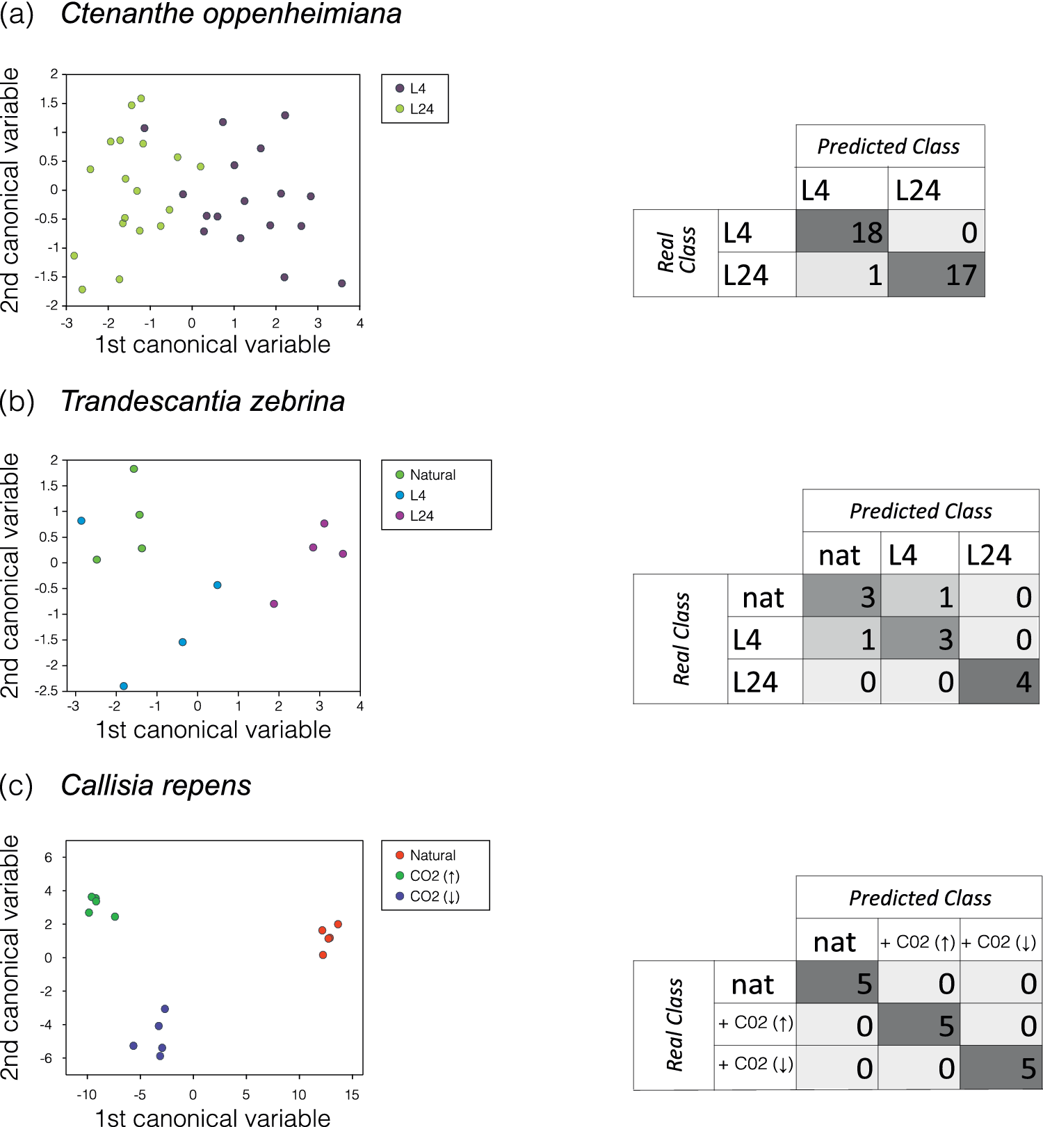
On the left side of Figure 4, the dimensional projection obtained from the canonical variable analysis (CVA) for the feature vectors with the highest accuracy for each species is presented, along with the confusion matrix on the right. From top to bottom, the vectors and rules used were:
$[\vec {\mu }_{S},\vec {\mu }_{W},\vec {\mu }_{L}]$
 with rule B57-S378 (Ctenanthe oppenheimiana),
$[\langle \mu _S\rangle ,\langle \mu _W\rangle ,\langle \mu _L\rangle ]$
 with rule B12345-S0456 (Tradescantia zebrina) and
$\vec {\mu }_S$
 with rule B014-S04567 (Callisia repens). These figures clearly demonstrate a distinct separation among the three network models, supporting the high success rates. Additionally, the L24 class is linearly separable from the others, while the natural and L4 classes are often confused, as indicated by the confusion matrix, which aligns with the high similarity of these stomata images in Figure 2b.
Two-dimensional projection obtained from the analysis of canonical variables and the corresponding confusion matrix for the highest accuracy rate. (a) CVA of the vector
$[\vec {\mu }_{S},\vec {\mu }_{W},\vec {\mu }_{L}]$
 with rule B57-S378 for the species Ctenanthe oppenheimiana. (b) CVA of the vector
$[\langle \mu _S\rangle ,\langle \mu _W\rangle ,\langle \mu _L\rangle ]$
 with rule B12345-S0456 for classifying the species Tradescantia zebrina. (c) CVA of the vector
$\vec {\mu }_S$
 using rule B014-S04567 for the species Callisia repens. In the confusion matrix, each cell indicates the number of correctly predicted instances.

Figure 4. Long description
The figure consists of three rows labeled a, b, and c.
Row a, Ctenanthe oppenheimiana:
The scatter plot on the left shows the 1st canonical variable on the x-axis (range -3 to 4) and the 2nd canonical variable on the y-axis (range -2 to 2). Data points for L 4 (dark purple) and L 24 (light green) show significant overlap in the center, though L 24 is more concentrated on the left. The confusion matrix on the right shows Real Class versus Predicted Class. For L 4, 18 were correctly predicted and 0 were misclassified. For L 24, 17 were correctly predicted and 1 was misclassified as L 4.
Row b, Tradescantia zebrina:
The scatter plot shows the 1st canonical variable (range -3 to 4) and the 2nd canonical variable (range -2.5 to 2). Three groups are plotted: Natural (green), L 4 (blue), and L 24 (magenta). The groups show distinct clustering with some proximity between Natural and L 4. The confusion matrix shows: for Natural (nat), 3 correct and 1 misclassified as L 4; for L 4, 3 correct and 1 misclassified as nat; for L 24, 4 correct and 0 misclassified.
Row c, Callisia repens:
The scatter plot shows the 1st canonical variable (range -10 to 15) and the 2nd canonical variable (range -6 to 6). Three highly distinct, non-overlapping clusters are visible: Natural (red) on the far right, C O sub 2 up-arrow (green) on the top left, and C O sub 2 down-arrow (blue) on the bottom left. The confusion matrix reflects 100 percent accuracy: 5 correct for nat, 5 correct for + C O sub 2 up-arrow, and 5 correct for + C O sub 2 down-arrow, with zeros in all off-diagonal cells.
3.3. Robustness analysis
To provide further intuition into the discriminative power of the LLNA, we analysed the features in the high-dimensional space. Figure 5 presents a pairplot of five representative descriptors for Callisia repens. Given the high dimensionality of the full feature vector (320 descriptors), only the first five were selected for this visualization. The diagonal plots show the estimated probability density for each individual descriptor, while the scatter plots illustrate how they combine to form well-separated clusters. Although the raw TEPs may appear stochastic and are not shown here – visual examples can be found in Miranda et al. (Reference Miranda, Machicao and Bruno2016), Neiva and Bruno (Reference Neiva and Bruno2023), Ribas et al. (Reference Ribas, Machicao and Bruno2020) and Zielinski et al. (Reference Zielinski, Ribas, Machicao and Bruno2024) – these statistical measures confirm the separability of the classes, demonstrating that the LLNA signatures are highly sensitive to the topological patterns induced by environmental stress.
Pairplot analysis of the first five descriptors for Callisia repens using the best-performing rule (B014-S04567 with
$\vec {\mu _S}$
 ). The diagonal plots show the density distribution for each descriptor, while the scatter plots illustrate pairwise relationships.

Figure 5. Long description
A multi-panel grid containing 25 individual plots. The diagonal from top-left to bottom-right features density distribution curves for five descriptors labeled mu s sub 1, mu s sub 2, mu s sub 3, mu s sub 4, and mu s sub 5. Each plot contains three color-coded distributions: red for Natural, green for C O sub 2 up arrow, and blue for C O sub 2 down arrow.
* The diagonal density plots show that mu s sub 1 has a sharp peak for Natural conditions around 0.55, while mu s sub 4 and mu s sub 5 show highly skewed distributions with Natural conditions peaking near zero.
* The off-diagonal scatter plots illustrate pairwise correlations.
* In the first column, mu s sub 1 is plotted against the other four descriptors. Green points (C O sub 2 up arrow) cluster at lower mu s sub 1 values (0.4 to 0.5) and higher mu s sub 3 and mu s sub 4 values.
* Blue points (C O sub 2 down arrow) and red points (Natural) tend to cluster at higher mu s sub 1 values (0.5 to 0.6).
* A legend in the bottom-right panel identifies the three groups: a red dot for Natural, a green dot for C O sub 2 up arrow, and a blue dot for C O sub 2 down arrow.
* The x-axes and y-axes are scaled specifically for each descriptor: mu s sub 1 ranges from 0.4 to 0.6, mu s sub 2 from 0.0 to 0.3, mu s sub 3 from 0.00 to 0.10, mu s sub 4 from 0.00 to 0.04, and mu s sub 5 from 0.000 to 0.030.
3.4. Baseline comparison
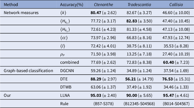
Table 3 compares the accuracy rates obtained by the LLNA with those from traditional structural network measurements and graph-based methods (Section 2.7).
Classification performance comparison
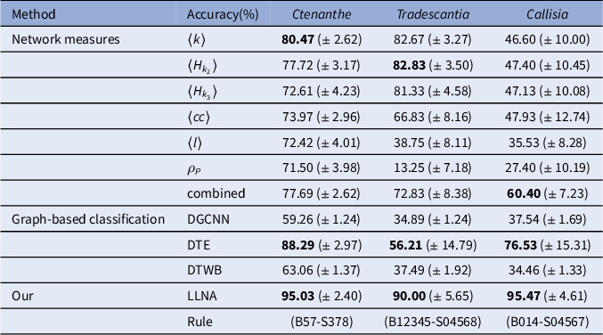
Table 3 Long description
The table is organized into five columns: Method, Accuracy percentage, Ctenanthe, Tradescantia, and Callisia.
Under the Network measures category:
- Average k: Ctenanthe 80.47 plus or minus 2.62, Tradescantia 82.67 plus or minus 3.27, Callisia 46.60 plus or minus 10.00.
- Average H sub k 2: Ctenanthe 77.72 plus or minus 3.17, Tradescantia 82.83 plus or minus 3.50, Callisia 47.40 plus or minus 10.45.
- Average H sub k 3: Ctenanthe 72.61 plus or minus 4.23, Tradescantia 81.33 plus or minus 4.58, Callisia 47.13 plus or minus 10.08.
- Average c c: Ctenanthe 73.97 plus or minus 2.96, Tradescantia 66.83 plus or minus 8.16, Callisia 47.93 plus or minus 12.74.
- Average l: Ctenanthe 72.42 plus or minus 4.01, Tradescantia 38.75 plus or minus 8.11, Callisia 35.53 plus or minus 8.28.
- rho sub P: Ctenanthe 71.50 plus or minus 3.98, Tradescantia 13.25 plus or minus 7.18, Callisia 27.40 plus or minus 10.19.
- combined: Ctenanthe 77.69 plus or minus 2.62, Tradescantia 72.83 plus or minus 8.38, Callisia 60.40 plus or minus 7.23.
Under the Graph-based classification category:
- D G C N N: Ctenanthe 59.26 plus or minus 1.24, Tradescantia 34.89 plus or minus 1.24, Callisia 37.54 plus or minus 1.69.
- D T E: Ctenanthe 88.29 plus or minus 2.97, Tradescantia 56.21 plus or minus 14.79, Callisia 76.53 plus or minus 15.31.
- D T W B: Ctenanthe 63.06 plus or minus 1.37, Tradescantia 37.49 plus or minus 1.92, Callisia 34.46 plus or minus 1.33.
Under the Our category:
- L L N A: Ctenanthe 95.03 plus or minus 2.40, Tradescantia 90.00 plus or minus 5.65, Callisia 95.47 plus or minus 4.61.
- Rule: Ctenanthe B 5 7 minus S 3 7 8, Tradescantia B 1 2 3 4 5 minus S 0 4 5 6 8, Callisia B 0 1 4 minus S 0 4 5 6 7.
combined
$[\langle k\rangle , \langle H_{k_2}\rangle , \langle H_{k_3}\rangle , \langle cc\rangle , \langle l\rangle , \rho _P]$

Note: Accuracy rates (%) and standard deviations for identifying phenotypic plasticity using traditional network structural measures, graph-based methods (DGCNN, DTE and DTWB) and the proposed LLNA approach (best-performing rules).
Regarding traditional network measurements, for Ctenanthe oppenheimiana, LLNA showed a classification increment of
$14.56$
 (
$\pm \, 3.55$
 ) percentage points compared to the average degree (
$\langle k\rangle $
 ), which obtained
$80.47$
 (
$\pm \, 2.62$
 )%. For Callisia repens, LLNA yielded a higher accuracy by
$35.07$
 (
$\pm \, 8.57$
 ) percentage points compared to the combination of measures that achieved
$60.40$
 (
$\pm \, 7.23$
 )%. Finally, for Tradescantia zebrina, LLNA presented an absolute gain of
$7.17$
 (
$\pm \, 6.64$
 ) percentage points compared to the hierarchical degree (
$\langle H_{k_2}\rangle $
 ), which yielded
$82.83$
 (
$\pm \, 3.50$
 )%. In these three scenarios, the results suggest that the dynamical signatures of the LLNA can capture topological nuances of phenotypic plasticity that may be less evident in static network metrics.
Regarding the three graph-based classification methods: DGCNN (Zhang et al., Reference Zhang, Cui, Neumann and Chen2018), DTWB (Merenda & Bruno, Reference Merenda and Bruno2023) and DTE (Scabini et al., Reference Scabini, Ribas, Ribeiro and Bruno2022), the results in Table 3 indicate that LLNA shows competitive accuracy rates when evaluated against these graph-based methods across the three studied species. When compared to the DTE method, which was the most competitive among them in our tests , LLNA yielded higher accuracy margins. Specifically, LLNA presented a gain over DTE by
$6.74$
 (
$\pm \, 3.82$
 ) percentage points for Ctenanthe oppenheimiana, and by margins of
$33.79$
 (
$\pm \, 15.83$
 ) and
$18.94$
 (
$\pm \, 15.99$
 ) percentage points for Tradescantia zebrina and Callisia repens, respectively.
The DGCNN and DTWB methods showed limited effectiveness in identifying the stress conditions, with accuracy rates often close to random guessing. The architectural complexity of deep frameworks like DGCNN easily leads to overfitting due to the severe imbalance between their large weight space and the small sample size available in this study. For DTWB, this performance might be explained by its original tuning on Watts--Strogatz networks, a specific topology that may not reflect the empirical distribution of our biological data. In contrast, while the DTE method performed better by using topological descriptors, it still exhibited high instability, as seen in the large standard deviations. The LLNA framework, by capturing the rules of network evolution as a deterministic feature extractor, appears to obtain stable patterns that are well-suited for these restricted data conditions.
4. Discussion
We analysed stomata distribution patterns by constructing stomata networks based on the distance matrix between pairs of stomata derived from microscopic images (Figure 2).
Regarding the network modelling, the connectivity of the network vertices (stomata) depends on the distance information and a threshold
$\delta _{T_{l}}$
 , with connectivity increasing as the threshold rises until the network becomes fully connected. The distance matrix for all pairs of stomata provides valuable insights into the geometry of the plant leaf, revealing correlations between the environment and its stomatic distribution structure (geometry). Notably, the specific threshold values used here do not limit the application of the method to other species or imaging setups. The fundamental requirement for the LLNA is the coverage of a broad spectrum of connectivity – from a nearly disconnected state to a highly connected one. This multi-scale approach allows the automata dynamics to characterize the spatial complexity of the distribution; therefore, researchers can adapt these ranges to their specific resolution, provided that this topological progression is maintained.
While the exhaustive search for rules in the LLNA framework adds an initial computational layer, this selection is a one-time training phase. Once the optimal rules are identified, feature extraction and classification become computationally efficient. In our study, LLNA presented higher accuracy margins than the selected graph models (DGCNN, DTE and DTWB) under small-sample constraints, supporting the observation that while deep learning models often need very large datasets to work well, the LLNA can be a suitable alternative for biological data with few samples. Notably, the 400 optimal rules, derived from only two images of Tradescantia zebrina, generalized to the other two species without re-optimization. This indicates that these rules capture shared structural patterns related to stomatal distribution within the evaluated cases, instead of just learning the specific details of one dataset. Consequently, the proposed approach shows promise for small-sample biological datasets, where network dynamics can effectively capture relevant patterns despite data limitations.
From the perspective of pattern recognition, the method effectively captures the unique characteristics of the three species. The maximum accuracy achieved by LLNA consistently surpasses both structural network measures and graph-based classification methods. Specifically, for Tradescantia zebrina, we attained an accuracy of
$90$
 (
$\pm \, 5.65$
 )%, despite the inherent difficulty in distinguishing natural and 4-h classes, as indicated by canonical analysis and the confusion matrix (Figure 4b). For Ctenanthe oppenheimiana, a similar high accuracy was observed, with only one sample misclassified. In the case of Callisia repens, we achieved excellent class separability.
From a biological standpoint, we observed that the stomata density (Figures 2a and b) is highly dependent on photoperiods, where longer exposure to light correlates with increased density. Similarly, for Callisia repens, the stress induced by
$\text {CO}_2$
 injection also influences stomata density, making the
$\text {CO}_2$
 (
$\uparrow $
 ) and
$\text {CO}_2$
 (
$\downarrow $
 ) classes challenging to differentiate using purely structural metrics.
Regarding plant plasticity, the LLNA approach helps to identify subtle changes in how stomata are organized. While traditional metrics often miss the complex spatial relationships between pores, the network automata can detect specific patterns caused by environmental stress. By measuring how these distributions change – from sparse to clustered or highly connected – the method provides a reliable way to evaluate these structural variations. This helps to show how plants adjust their leaf surface for gas exchange under different environmental conditions.
Such topological distribution analysis can be a valuable tool for monitoring environmental changes in natural ecosystems, as stomatal density alone is already used to model how plants sense and drive global changes (Cai & Cao, Reference Cai and Cao2004; Hetherington & Woodward, Reference Hetherington and Woodward2003). Therefore, precise spatial frameworks like LLNA offer a non-destructive strategy to track human-induced climate impacts on biomes over time. This approach is particularly advantageous for live leaves of species with a purple abaxial epidermis -- such as those studied here (de Almeida Filho, Reference de Almeida Filho2018) – since distance metrics can be preserved and analysed without prior histological processing. Additionally, this methodology can be extended to agricultural sciences to evaluate crop adaptation to different fertilization, irrigation and local climatic regimes.
Despite these achievements, the dataset’s limitations must be acknowledged. Compiling a comprehensive biological dataset was inherently challenging due to the meticulous time constraints required for controlled plant cultivation and monitoring. It is worth noting that while the LLNA framework was originally designed with large datasets in mind (Miranda et al., Reference Miranda, Machicao and Bruno2016), evaluating its performance under these restricted sample sizes was a deliberate test of its versatility. The positive results observed here suggest a promising adaptability to data-scarce scenarios, although further extensive testing remains necessary. Future research should focus on automated methods for processing leaf images and expanding the datasets to include more species to further enhance the robustness and validate the generalizability of our approach.
Finally, the development of these computational tools remains essential for expanding our understanding of ecological and agricultural resilience. In this context, our findings suggest the feasibility of the LLNA as an effective pattern recognition tool to quantify the phenotypic plasticity of stomatal distribution in response to environmental stressors.
Open peer review
To view the open peer review materials for this article, please visit http://doi.org/10.1017/qpb.2026.10051.
Acknowledgements
We would like to thank the Scientific Computing Group of the São Carlos Institute of Physics for providing the stomatal image dataset.
Author contributions
All authors contributed synergistically to the different stages of the research project. More specifically:
Conceptualization: J.M., H.A.d.A.F. and O.M.B.; Data curation: J.M. and H.A.d.A.F.; Formal analysis: J.M.; Investigation: J.M. and H.A.d.A.F.; Methodology: J.M. and H.A.d.A.F.; Software: J.M. and K.Z.; Supervision: O.M.B.; Validation: J.M. and H.A.d.A.F.; Visualization: J.M.; Writing – original draft: J.M. and H.A.d.A.F.; Writing – review and editing: J.M. All authors have read and agreed to the published version of the manuscript.
Competing interests
There are no competing interests to declare.
Data availability statement
A zip file containing the images dataset and centroid files for each of the three species can be found in de Almeida Filho & Machicao (Reference de Almeida Filho and Machicao2026) https://doi.org/10.5281/zenodo.18567387. The source code for the LLNA feature extraction and the classification pipeline is now available at https://github.com/machicao/stomata-LLNA.
Funding statement
This research received no specific grant from any funding agency, commercial or not-for-profit sectors.
Disclosure statement
This manuscript has not been published nor is it under consideration by any other journal. There are no financial obligations with governmental or private organizations that can affect the content, results or conclusions of the present manuscript.
Declaration of generative AI in the writing process
During the preparation of this work, the authors used Gemini to enhance text clarity and flow. The authors thoroughly reviewed and edited the final content and take full responsibility for the published article.
Supplementary material
The supplementary material for this article can be found at https://doi.org/10.1017/qpb.2026.10051.








 Open access


Comments
The current context of climate change and the adaptations that living beings acquire to exist in a stressful environment make this work worthy of review by the scientific community. We developed a new computational strategy to measure the plasticity of stomatal distribution in leaves under directed environmental changes. This strategy, we assume, is a powerful computational tool to ascertain patterns of stomatal distribution on the surface of leaves. The literature shows that stomatal adaptation is fundamental for the establishment and survival of a plant in a variable environment. At the same time, stomata are largely responsible for the geochemical cycles of water and carbon flux on planet Earth. Therefore, evaluating a new strategy to measure adaptations of stomatal distribution is fundamental for plant science and for a humanity suffering from the climatic consequences of its actions on the planet.