
1. Introduction
Dip coating is a common industrial coating method that consists in withdrawing a substrate from a liquid bath at a constant speed (Ruschak Reference Ruschak1985; Scriven Reference Scriven1988; Quéré Reference Quéré1999; Grosso Reference Grosso2011). This method has been studied since 1942 by Levich & Landau (Reference Levich and Landau1942) and Derjaguin (Reference Derjaguin1943) in the configuration of a plate withdrawn at a constant velocity  $U$ from a Newtonian liquid of viscosity
 $\eta$, density
 $\rho$ and surface tension
 $\gamma$. Far from the liquid bath, the thickness
 $h$ of the liquid film coating the plate is uniform and set by the balance of viscous stresses, which enable the plate to pull the liquid out of the bath, and capillary stresses at the meniscus, which pull the fluid back to the bath (Rio & Boulogne Reference Rio and Boulogne2017). The relative magnitude of viscous stresses to capillary stresses at the meniscus is measured by the capillary number,
 ${Ca}=\eta U/\gamma$. In the limit of small capillary number
 ${Ca} \ll 1$ and small Reynolds number
 ${Re} =\rho U h/\eta \ll 1$, the thickness of the coating film is given by the Landau–Levich–Derjaguin (LLD) law
 \begin{equation} h=0.94 \ell_c {Ca}^{2/3}, \end{equation}
where  $\ell _c=\sqrt {\gamma /(\rho g)}$ is the capillary length, and where g is a gravitational constant,
 $g = 9.81\ \textrm{m s}^{-2}$. At larger capillary numbers, typically of the order of
 $Ca \gtrsim 10^{-2}$, gravity dominates capillary forces (Maleki et al. Reference Maleki, Reyssat, Restagno, Quéré and Clanet2011). The balance between viscosity and gravity leads to a new scaling law for the thickness of the liquid film coating a plate,
 $h \propto \ell _c {Ca}^{1/2}$.
Owing to the complexity of the fluids used in industrial processes, various studies have considered the dip-coating of homogeneous fluids with complex rheology, such as shear-thinning fluids (Gutfinger & Tallmadge Reference Gutfinger and Tallmadge1965; Hewson, Kapur & Gaskell Reference Hewson, Kapur and Gaskell2009), yield-stress fluids (Maillard, Boujlel & Coussot Reference Maillard, Boujlel and Coussot2014, Reference Maillard, Boujlel and Coussot2015; Smit et al. Reference Smit, Kusina, Joanny and Colin2019), viscoelastic fluids (Ro & Homsy Reference Ro and Homsy1995; De Ryck & Quéré Reference De Ryck and Quéré1998; Ruckenstein Reference Ruckenstein2002) as well as the influence of surfactants (Shen et al. Reference Shen, Gleason, McKinley and Stone2002; Krechetnikov & Homsy Reference Krechetnikov and Homsy2006; Delacotte et al. Reference Delacotte, Montel, Restagno, Scheid, Dollet, Stone, Langevin and Rio2012), roughness (Krechetnikov & Homsy Reference Krechetnikov and Homsy2005; Seiwert, Clanet & Quéré Reference Seiwert, Clanet and Quéré2011) and the geometry of the substrate (White & Tallmadge Reference White and Tallmadge1965; Zhang et al. Reference Zhang, Salamatin, Peng and Kornev2022). Suspensions, in which solid particles are dispersed in a liquid phase, are of particular interest to manufacturing applications. Indeed, the particles can give specific properties to a surface after coating. Thus, dip coating, in particular combined with evaporation, has been considered for optical applications, self-assembling of particles and wettability treatments (Ghosh, Fan & Stebe Reference Ghosh, Fan and Stebe2007; Mechiakh et al. Reference Mechiakh, Ben Sedrine, Chtourou and Bensaha2010; Berteloot et al. Reference Berteloot, Daerr, Lequeux and Limat2013; Mahadik et al. Reference Mahadik, Vhatkara, Mahadik, Kavale, Wagh, Gupta and Gurav2013). More recently, several studies have considered the dip coating of monodisperse suspensions (single particle size), of non-Brownian particles (diameter  $d$ larger than a few tens of microns), in non-volatile liquids (Kao & Hosoi Reference Kao and Hosoi2012; Gans et al. Reference Gans, Dressaire, Colnet, Saingier, Bazant and Sauret2019; Palma & Lhuissier Reference Palma and Lhuissier2019). These studies revealed that, depending on the withdrawal velocity
 $U$, the fluid properties and the size of the particles, three different coating regimes are observed: (i) at small withdrawal velocity, a thin film is deposited without any particles in it; (ii) at large withdrawal velocity (i.e. large capillary numbers), the entrained film contains particles, and its thickness follows the Landau–Levich law using at first order the effective viscosity of the suspension; finally (iii) at intermediate withdrawal velocities, the coating is heterogeneous, with an average film thickness that corresponds to a monolayer of particles and remains roughly constant over a range of capillary numbers. For a monodisperse suspension, the transition between the different regimes is governed by the thickness of the coating film relative to the particle diameter
 $h/d$ (Gans et al. Reference Gans, Dressaire, Colnet, Saingier, Bazant and Sauret2019; Palma & Lhuissier Reference Palma and Lhuissier2019).
The transition between the no-particle and heterogeneous coating regime also depends on the accumulation of particles at the meniscus. This transition is therefore complex to predict quantitatively for non-dilute suspensions, typically as soon as the volume fraction, defined as  $\phi =V_{p}/(V_{p}+V_{l})$, where
 $V_{p}$ and
 $V_{l}$ are the volume of particles and liquid, respectively, is larger than a few per cent. The configuration of isolated particles is simpler to describe because the particles do not interact with each other. This configuration was considered for flat plates (Colosqui, Morris & Stone Reference Colosqui, Morris and Stone2013; Sauret et al. Reference Sauret, Gans, Colnet, Saingier, Bazant and Dressaire2019) and fibres (Dincau et al. Reference Dincau, Mai, Magdelaine, Lee, Bazant and Sauret2020). The two-dimensional numerical study of Colosqui et al. (Reference Colosqui, Morris and Stone2013) has shown that an isolated particle can be entrained in the coating film if the particle diameter
 $d$ is smaller than the thickness at the stagnation point
 $h^*$. Indeed, the stagnation point defines the boundary between a shear flow, where the fluid continues into the coating film, and a recirculation flow, where the fluid returns into the liquid bath. Thus, the thickness
 $h^*$ controls the entrainment of particles in the coating film. The value of
 $h^*$ is related to the thickness of the coating film through
 ${h^{*}}/{\ell _{c}}=3 {h}/{\ell _{c}}-({h}/{\ell _{c}})^{3}$ (Levich & Landau Reference Levich and Landau1942), which in the limit of small capillary numbers becomes
 $h^{*}=3h$. Experiments with monodisperse spherical particles, have demonstrated that the entrainment of isolated particles occurs when the particle radius is roughly smaller than the thickness of the stagnation point (Sauret et al. Reference Sauret, Gans, Colnet, Saingier, Bazant and Dressaire2019)
 \begin{equation} h^{*}=3 h\gtrsim d/2. \end{equation}
The ability to control the film thickness, and thus the thickness at the stagnation point, by simply tuning the withdrawal velocity  $U$ has led to a method for sorting particles by size through dip coating (Dincau et al. Reference Dincau, Bazant, Dressaire and Sauret2019). This study has considered dilute suspensions and has shown that, since smaller particles can be entrained for smaller coating thickness, isolated particles can be separated by size via selecting an appropriate withdrawal velocity.
This entrainment process is not specific to dip coating. The translation of an air bubble in a tube, as well as the withdrawal of the fluid leading to the deposition of a thin film on the wall of a capillary tube, share many common features with the dip-coating configuration, in particular, the presence of a stagnation point (Bretherton Reference Bretherton1961; Krechetnikov Reference Krechetnikov2010). Therefore, similar observations on the entrainment of particles (Jeong et al. Reference Jeong, Kvasnickova, Boutin, Cébron and Sauret2020; Wu et al. Reference Wu, Yang, Hu, Chen, Zhong, Yang and Jin2021) and the filtering of particles (Yu, Khodaparast & Stone Reference Yu, Khodaparast and Stone2018) have been reported. We should also emphasize that the influence of particles on different interfacial phenomena, such as the formation of droplets (Furbank & Morris Reference Furbank and Morris2004; Bonnoit et al. Reference Bonnoit, Bertrand, Clément and Lindner2012; Château, Guazzelli & Lhuissier Reference Château, Guazzelli and Lhuissier2018; Thiévenaz & Sauret Reference Thiévenaz and Sauret2021), jets (Château & Lhuissier Reference Château and Lhuissier2019) and liquid sheets (Raux et al. Reference Raux, Troger, Jop and Sauret2020), has also reported that the critical length scale at which the particles start to modify significantly the dynamics is comparable to the diameter of the particles.
Whereas most of these studies have considered the ideal situation of a suspension made of monodisperse particles, many industrial and environmental processes involve polydisperse particles with a wide range of sizes. It is known that for a given solid volume fraction, a polydisperse suspension will be less viscous than its monodisperse counterpart (Shapiro & Probstein Reference Shapiro and Probstein1992). For dip coating, the size distribution of the particles also needs to be compared with the thickness of the coating film. It remains unclear how the three regimes reported previously for monodisperse suspensions will need to be modified to account for the polydispersity of the suspension.
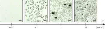
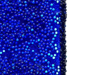
Figure 1 shows four examples of coating films on a plate withdrawn from a bidisperse suspension when increasing the withdrawal velocity  $U$. The suspension contains particles of diameter
 $d_L=250\ \mathrm {\mu }{\rm m}$ and
 $d_{S}=80\ \mathrm {\mu }{\rm m}$, at a volume fraction of
 $\phi =0.2$. The volume ratio of large particles is
 $\zeta =V_{L}/(V_{L}+V_{S})=0.6$, where
 $V_{L}$ and
 $V_{S}$ are the volumes of large and small particles in the suspension, respectively. The main features observed for monodisperse suspensions are also observed with bidisperse suspensions. In particular, at very low withdrawal velocity (
 $U=0.01\ {\rm mm}\ {\rm s}^{-1}$), the particles remain in the liquid bath as they are much larger than the coating film. As a result, the meniscus filters them out, and the thin film is only made of liquid. At large withdrawal velocities (
 $U=10\ {\rm mm}\ {\rm s}^{-1}$) we observe an effective viscosity regime. Both populations of particles are present, in proportions similar to the suspension in the bath. At intermediate withdrawal velocities, a behaviour specific of bidisperse suspensions is observed. Initially, at low withdrawal velocity (
 $U=0.1\ {\rm mm}\ {\rm s}^{-1}$), only small particles are present in the coating film. When increasing the withdrawal velocity (
 $U=1\ {\rm mm}\ {\rm s}^{-1}$), the thickness of the coating film also increases, resulting in more and more large particles being entrained in the film. As a result, the composition of the coating film differs from that of the bath in this regime, with varying proportions of small and large particles depending on the withdrawal velocity.
Typical coating films observed on a flat plate for increasing withdrawal velocities for a bidisperse suspension of particles of diameter  $d_{L}= 250\ \mathrm {\mu }{\rm m}$ and
 $d_{S}= 80\ \mathrm {\mu }{\rm m}$ (size ratio
 $\delta =3.125$), at a volume fraction of
 $\phi =0.2$ and a volume ratio of large particles
 $\zeta =0.6$. The withdrawal velocity
 $U$ increases from left to right:
 $U=0.01, 0.1, 1$ and
 $10\ {\rm mm}\ {\rm s}^{-1}$. The size of the scale bars is
 $500\ \mathrm {\mu }\rm {m}$.

In this study, we aim to describe the evolution of the thickness and the composition of the coating film when varying the capillary number and the composition of the suspension. As a first step towards polydisperse systems, we consider bidisperse suspensions made of small and large particles of diameter  $d_{S}$ and
 $d_{L}$, respectively. The volume ratio of large to small particles is varied to probe the influence of the size distribution of particles on the formation and composition of the coating film. This paper is organized as follows: the experimental methods and the suspensions used are first presented in § 2. Dip coating with monodisperse suspensions is recalled in § 3, notably to refine the measurements of the thickness of the coating film. Indeed, in the effective viscosity regime, we show that the volume fraction in the film is slightly smaller than in the suspension bath. Section 4 is devoted to the experimental characterization with bidisperse suspensions. We describe and rationalize the different regimes observed and show that, in the thick-film regime, rheological models developed for bidisperse suspensions enable us to model the thickness of the coating film, while the heterogeneous regime is more complex for bidisperse suspensions. We show that the composition of the coating film evolves with the withdrawal velocity, and we propose a model that captures the evolution of the composition of the coating film, in particular, the filtration of large particles at intermediate velocities.
2. Experimental methods
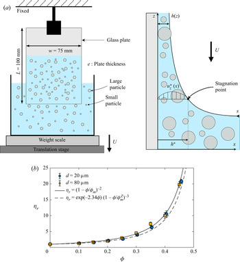
Our experiments consist in withdrawing a glass plate ( $w=75\ \textrm {mm}$ wide and
 $e=3.25\ \textrm {mm}$ thick) from a rectangular container (width 108 mm and thickness 35 mm) filled with a particulate suspension. Figure 2(a) shows a schematic of the experimental set-up. The suspensions are prepared by dispersing the non-Brownian particles in a silicone oil having a density close to the density of the particles. The particles used are spherical polystyrene particles (Dynoseeds TS from Microbeads) with diameters
 $d = 22, 81, 145$ and
 $249\ \mathrm {\mu }\rm {m}$ (later referred as
 $d = 20, 80, 140$ and
 $250\ \mathrm {\mu }\rm {m}$) and densities between
 $1046$ and
 $1062\ {\rm kg}\ {\rm m}^{-3}$ depending on the batch (see the physical characterization in the Appendix). The silicone oil (AP100, Sigma-Aldrich) has a viscosity of
 $\eta _0 = 112\ {\rm mPa}\ {\rm s}$, density
 $\rho = 1058\ {\rm kg}\ {\rm m}^{-3}$ and a surface tension of
 $\gamma =25 \pm 2\ {\rm mN}\ {\rm m}^{-1}$ at
 $20\,^{\circ }$C. Silicone oil perfectly wets the plate and the particles and is used for dip-coating experiments to avoid any potential effects from surfactants, which are known to increase the thickness of the coating film even at low concentrations (Krechetnikov & Homsy Reference Krechetnikov and Homsy2005, Reference Krechetnikov and Homsy2006; Rio & Boulogne Reference Rio and Boulogne2017). The surface tension of the suspension is equal to that of the suspending liquid, i.e. it is not affected by the volume fraction or by the size of the suspended particles (Couturier et al. Reference Couturier, Boyer, Pouliquen and Guazzelli2011; Château et al. Reference Château, Guazzelli and Lhuissier2018; Zhao et al. Reference Zhao, Oléron, Pelosse, Limat, Guazzelli and Roché2020). The particles are first dispersed using a paint mixer. Then, the suspension is left in a vacuum chamber for a few minutes to remove any entrapped bubble in the suspension. Between each experiment, the suspension is re-homogenized to ensure that the settling of the particles is negligible at the time scale of one experiment (typically a few minutes).
(a) Schematic of the experimental set-up. Front (left) and side views (right). (b) Relative effective shear viscosity  $\eta _{r}=\eta /\eta _0$ of monodisperse suspensions for particles of diameter
 $d=20\ \mathrm {\mu }{\rm m}$ (blue circles) and
 $d=80\ \mathrm {\mu }{\rm m}$ (yellow squares). The solid line indicates the Maron–Pierce correlation ((2.2) with
 $\phi _m=0.58$), and the dashed line is the Zarraga correlation ((2.3) with
 $\phi _m^Z=0.62$).

The liquid bath is placed on a stage that is translated vertically using a stepper motor (Thorlabs NRT150) at a given velocity  $0.01\ {\rm mm}\ {\rm s}^{-1} < U<15\ {\rm mm}\ {\rm s}^{-1}$. Such an approach avoids mechanical perturbations that could influence the thickness of the coating film (Maleki et al. Reference Maleki, Reyssat, Restagno, Quéré and Clanet2011). After the plate has been withdrawn from the liquid bath, pictures of the coating film are taken using a DSLR camera (Nikon D5600) equipped with a macro lens (Nikkor 200 mm). A microscopic lens (Mitutoyo M Plan Apo 5X) is also used for suspensions of
 $d = 20\ \mathrm {\mu }{\rm m}$ particles. Between each experiment, the glass plate is thoroughly cleaned with isopropyl alcohol, rinsed multiple times with deionized water and then dried with compressed air.
In addition to directly observing the coating film, its thickness is estimated by a gravimetric method, chosen for its excellent accuracy (Krechetnikov & Homsy Reference Krechetnikov and Homsy2005). The liquid bath is placed on an analytical weighing scale (Ohaus SPX622 Scout, with an accuracy of  $0.01\ {\rm g}$) during the experiments. The translating stage is moved up until the plate is dipped in the suspension bath to the desired dipping length
 $L_1$, and then withdrawn, holding a mass of entrained fluid
 $m_1$. The plate is then dipped again to a larger length
 $L_2$, and then withdrawn while holding an increased fluid mass
 $m_2$ on the plate. The resulting average thickness of the deposited liquid film is then given by
 \begin{equation} h= \frac{m_2-m_1}{(L_2-L_1) \rho P}, \end{equation}
where  $P=2 (w+e)$ is the perimeter of the plate,
 $w$ is the width and
 $e$ the thickness of the plate and
 $\rho$ is the density of the suspension. Subscripts
 $1$ and
 $2$ denote the two dipping lengths such that
 $L_2>L_1$. This approach prevents a lower edge effect that interferes with the estimation of the film thickness (Krechetnikov & Homsy Reference Krechetnikov and Homsy2005). For the width of the plate, the dipping lengths and the scale used here, the uncertainty on the film thickness is of order
 $\pm 3\ \mathrm {\mu }{\rm m}$. More details on this method have been provided by Krechetnikov & Homsy (Reference Krechetnikov and Homsy2005).
The shear viscosity of the suspensions is measured using a dynamic shear rheometer (Anton Paar MCR92) with a 25 mm diameter plate–plate rough geometry and a gap of 1 mm between the plates. In the range of volume fraction considered here, the suspension has a Newtonian behaviour and is characterized by its shear viscosity  $\eta$. Figure 2(b) reports the evolution of the relative shear viscosity,
 $\eta _{r}(\phi )=\eta (\phi )/\eta _0$ for a volume fraction in the range
 $10\,\%<\phi <40\,\%$ and two particles sizes (
 $20\ \mathrm {\mu }{\rm m}$ and
 $80\ \mathrm {\mu }{\rm m}$, monodisperse suspensions). Many empirical correlations between
 $\eta _{r}$ and
 $\phi$ can be found in the literature (Quemada Reference Quemada1977; Stickel & Powell Reference Stickel and Powell2005; Dörr, Sadiki & Mehdizadeh Reference Dörr, Sadiki and Mehdizadeh2013; Guazzelli & Pouliquen Reference Guazzelli and Pouliquen2018). In the following, we use the Maron–Pierce correlation
 \begin{equation} \eta_{r}=\frac{\eta(\phi)}{\eta_0}=(1-\phi/\phi_{m})^{{-}2}, \end{equation}
where  $\phi _{m}$ corresponds to the volume fraction of particles at which the viscosity diverges. Fitting (2.2) to our measurements leads to
 $\phi _{m} \approx 0.58$, in agreement with other measurements performed in the literature with the same particles (Château et al. Reference Château, Guazzelli and Lhuissier2018; Guazzelli & Pouliquen Reference Guazzelli and Pouliquen2018). Note that other correlations can be used. For instance, the Zarraga correlation (Zarraga, Hill & Leighton Reference Zarraga, Hill and Leighton2000) has been used to describe the dip coating of monodisperse suspensions (Gans et al. Reference Gans, Dressaire, Colnet, Saingier, Bazant and Sauret2019), the pinch-off of suspension droplets (Bonnoit et al. Reference Bonnoit, Bertrand, Clément and Lindner2012) and the flow of suspensions on an inclined plane (Bonnoit et al. Reference Bonnoit, Darnige, Clement and Lindner2010). The Zarraga correlation is given by
 \begin{equation} \eta_r=\frac{\eta(\phi)}{\eta_0}=\frac{\exp ({-}2.34 \phi)}{(1-\phi / \phi_{m}^{\rm Z})^{3}}, \end{equation}
which leads with our measurements to  $\phi _{m}^{Z}=0.62$, also in agreement with the values reported in other studies (Bonnoit et al. Reference Bonnoit, Bertrand, Clément and Lindner2012). The Zarraga correlation slightly underestimates the effective shear viscosity for
 $\phi \gtrsim 0.25$ but better captures it at moderate volume fraction (
 $\phi \sim 0.1-0.2$). The Eilers correlation is also an option (Stickel & Powell Reference Stickel and Powell2005), and has been used recently for the spreading of suspension droplets (Zhao et al. Reference Zhao, Oléron, Pelosse, Limat, Guazzelli and Roché2020). Our decision to choose the Maron–Pierce correlation here is motivated by previous studies showing that the viscosity diverges as
 $(1-\phi /\phi_m)^{-2}$, stressing the exponent
 $-2$ (Guazzelli & Pouliquen Reference Guazzelli and Pouliquen2018).
For a given  $\phi$, the effective shear viscosity of a bidisperse suspension is lower than that of a monodisperse suspension (Shapiro & Probstein Reference Shapiro and Probstein1992; Probstein, Sengun & Tseng Reference Probstein, Sengun and Tseng1994; Gamonpilas, Morris & Denn Reference Gamonpilas, Morris and Denn2016; Guy et al. Reference Guy, Ness, Hermes, Sawiak, Sun and Poon2020). This effect is linked to the higher compacity of polydisperse sphere packings (Ouchiyama & Tanaka Reference Ouchiyama and Tanaka1984). Indeed, in a packing of polydisperse spheres, small particles can fill the interstices between the larger ones, which leads to a higher maximum packing fraction
 $\phi _{m}$. Compared with the monodisperse case, where
 $\eta$ is only a function of
 $\phi$, the viscosity of bidisperse suspensions depends on two additional parameters: the ratio of large to small particle diameters
 $\delta = d_{L}/d_{S}$, and the fraction of the solid volume occupied by the larger particles
 $\zeta = V_{L}/(V_{L} + V_{S})$ (Shapiro & Probstein Reference Shapiro and Probstein1992). Experimental measurements have shown that the viscosity of bidisperse suspensions follows the Maron–Pierce correlation, provided that
 $\phi _{m}$ takes the polydispersity into account (Thiévenaz, Rajesh & Sauret Reference Thiévenaz, Rajesh and Sauret2021).
3. Dip coating of monodisperse suspension
Monodisperse suspensions, i.e. composed of particles of a single size, are first considered for volume fractions ranging from  $\phi =10\,\%$ to
 $\phi =40\,\%$ and different particle diameters. The goal here is to verify whether the Maron–Pierce correlation (2.2) can predict the thickness of the coating films. Gans et al. (Reference Gans, Dressaire, Colnet, Saingier, Bazant and Sauret2019) and Palma & Lhuissier (Reference Palma and Lhuissier2019) have previously shown that, if the film is approximately thicker than the particle diameter (
 $h \gtrsim d$), its thickness follows the same law as a viscous liquid (1.1), where the viscosity corresponds to the effective viscosity of the suspension. However, despite a good agreement, this approach slightly overestimates the thickness of the coating film (see figures 5 and 8 in Gans et al. Reference Gans, Dressaire, Colnet, Saingier, Bazant and Sauret2019 for large volume fraction).
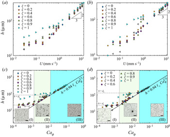
Figures 3(a) and 3(b) show the thickness of the coating film  $h$ when varying the withdrawal velocity of the plate
 $U$ for particles of diameter
 $20\ \mathrm {\mu }{\rm m}$ and
 $80\ \mathrm {\mu }{\rm m}$, respectively. As expected, the faster the withdrawal, the thicker the coating film. Besides, increasing the volume fraction of particles, and thus the viscosity of the suspension in the bath, also leads to thicker films. When
 $h \gtrsim d$, we observe the transition to the effective viscosity regime, in which
 $h \propto U^{2/3}$ according to the LLD law (1.1), in agreement with previous works (Gans et al. Reference Gans, Dressaire, Colnet, Saingier, Bazant and Sauret2019; Palma & Lhuissier Reference Palma and Lhuissier2019).
Thickness of the coating film as a function of (a,b) the withdrawal velocity  $U$, and of (c,d) the effective capillary number
 ${Ca}_{\phi }$, for varying volume fractions
 $\phi$ of particles of diameter (a–c)
 $d = 20\ \mathrm {\mu }{\rm m}$, and (b–d)
 $d = 80\ \mathrm {\mu }{\rm m}$. The thick continuous line is the LLD law (1.1) where the viscosity is considered as a fitting parameter. The horizontal dashed line in figures (c) and (d) corresponds to a coating film of thickness equals to the particle diameter (
 $h=d$). The coloured area in (c) and (d) corresponds to the effective viscosity regime.

To begin with, no assumption regarding the effective viscosity of the suspension is made. Instead, it is treated as a fitting parameter that we can estimate through the LLD law
 \begin{equation} h=0.94 \ell_c {{Ca}_\phi}^{2/3}=0.94 \ell_c \left(\frac{\eta(\phi) U}{\gamma}\right)^{2/3}. \end{equation}
The capillary number is based on the effective viscosity of the suspension:  ${Ca}_\phi =\eta (\phi ) U/\gamma$. In this expression, the capillary length
 $\ell _c$ and the surface tension
 $\gamma$ are physical properties of the liquid which are not modified by the particles,
 $U$ is the withdrawal velocity and
 $\eta (\phi )$ is the effective viscosity of the suspension. For each experiment,
 $\eta (\phi )$ is considered as a fitting parameter so that the thickness of the film in the LLD regime is captured quantitatively by (3.1).
We observe that, for both particle diameters ( $20\ \mathrm {\mu }{\rm m}$ and
 $80\ \mathrm {\mu }{\rm m}$), the experimental data collapse onto the LLD law when
 $h\gtrsim d$ (figure 3c,d). A similar observation can also be made for other sizes of particles used in this study. Figure 4(a) reports the relative effective viscosity of the suspension,
 $\eta _{r}=\eta (\phi )/\eta _0$ obtained through this approach. The evolution is similar for both particle sizes: at small enough volume fractions (
 $\phi \lesssim 0.2$), the viscosity follows the Mason–Pierce correlation (2.2) although it is slightly smaller than the viscosity of the suspension in the bath.
(a) Relative shear viscosity  $\eta _{r}$ of suspensions of particle diameter
 $d = 20\ \mathrm {\mu }{\rm m}$ and
 $d = 80\ \mathrm {\mu }{\rm m}$ as a function of the particle volume fraction in the bath
 $\phi$ (circles). Here,
 $\eta _{r}$ is estimated from the thickness of the coating film using (3.1). The shear viscosity measured with the rheometer is also reported (squares). The dashed line is the Maron–Pierce correlation (2.2). (b) Comparison between the particle volume fraction of the suspensions in the bath,
 $\phi$, and the value obtained from the viscosity
 $\phi _{meas}$, measured either by dip coating or rheometer. The dashed line corresponds to
 $\phi_{\textit{max}}=\phi$.

At larger volume fractions, the viscosity  $\eta (\phi )$ obtained by fitting the experimental data with the LLD law is systematically lower than the viscosity of the suspension in the bath. The larger difference in viscosity observed for larger volume fractions is due to the nonlinearity of the evolution of
 $\eta _{r}$ with
 $\phi$. The estimated value of
 $\eta (\phi )$ then allows us to calculate the corresponding volume fraction
 $\phi$ by using (2.2). The difference between the actual volume fraction of the suspension in the bath and the estimated volume fraction of the coating film is reported in figure 4(b). The difference is approximatively equal to
 ${\rm \Delta} \phi = 0.008, 0.012, 0.056, 0.049$ for
 $\phi =0.1, 0.2, 0.3, 0.4$, and thus shows a relative variation of
 ${\rm \Delta} \phi /\phi =8\,\%, 6\,\%, 18\,\%$ and
 $12\,\%$. The decrease in particle volume fraction in the coating film has been previously reported, yet it was of smaller magnitude (Palma & Lhuissier Reference Palma and Lhuissier2019). This small variation in volume fraction could be an effect of self-filtration due to the abrupt change in the flow at the stagnation point. This effect has been investigated by Kulkarni, Metzger & Morris (Reference Kulkarni, Metzger and Morris2010) for the gravity-driven flow of dense suspensions (
 $\phi >0.5$) through a wide aperture. Here, the stagnation point and the dynamic meniscus also play the role of an aperture, with one solid boundary and one deformable boundary imposed by the air–liquid interface, so that a similar self-filtration effect can be expected. Note that the resulting difference between the coating thickness and the predicted value by the LLD law and the Maron–Pierce correlation is small (approximately
 $10\,\%$) and was already visible in previous measurements (Gans et al. Reference Gans, Dressaire, Colnet, Saingier, Bazant and Sauret2019). We insist on this point to stress the difference between the viscosity decrease due to self-filtration and the viscosity decrease to polydispersity, which can be of similar magnitude. We should also emphasize that confinement effects are also known to influence the viscosity of suspension due to a change in the packing structure (Peyla & Verdier Reference Peyla and Verdier2011; Fornari et al. Reference Fornari, Brandt, Chaudhuri, Lopez, Mitra and Picano2016). Nevertheless, since a constant viscosity was measured for a range of coating thicknesses, as shown in figure 3, the influence of confinement effects on the decrease in viscosity is negligible here. In the following section, we consider the role of a bimodal distribution of particle size on the coating film.
4. Coating of bidisperse suspensions
4.1. General observations
In this section, we consider suspensions of particles having a bimodal size distribution: small particles of diameter  $d_{S}$ and large particles of diameter
 $d_{L}$. The composition of the solid phase is defined by the volume ratio of large particles:
 $\zeta =V_{L}/(V_{L}+V_{S})$, where
 $V_{L}$ and
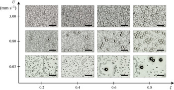
 $V_{S}$ are the volume of large and small particles in the suspension, respectively. Figure 5 shows examples of typical coating patterns observed for different withdrawal velocities
 $U$ and for different compositions of the solid phase, with
 $d_{S}=20\ \mathrm {\mu }{\rm m}$ and
 $d_{L}=80\ \mathrm {\mu }{\rm m}$. The solid volume fraction is kept constant and equal to
 $\phi =0.2$. We observe that the composition of the coating film changes drastically in terms of particle size distribution and depends both on
 $U$ and
 $\zeta$. For instance, for a balanced composition (
 $\zeta =0.4$) and a low withdrawal velocity, only the small particles are entrained in the coating film. For a given value of
 $\zeta$, the number of large particles increases with the withdrawal velocity, and thus the thickness
 $h$ of the film. We observe the same behaviour for all compositions of
 $\zeta$ considered here.
Examples of coating films observed for bidisperse suspensions of particles of diameter  $d_{S}=20\ \mathrm {\mu }{\rm m}$ and
 $d_{L}=80\ \mathrm {\mu }{\rm m}$ (size ratio
 $\delta =4$), at a volume fraction
 $\phi =0.2$ and different volume ratios of large particles (
 $\zeta =0.2, 0.4, 0.6$ and
 $0.8$) for increasing withdrawal velocity
 $U$. The size of the scale bars is 250
 $\mathrm {\mu }{\rm m}$.

A deficit of large particles in the coating film is observed for low or moderate withdrawal velocity. Indeed, when the thickness at the stagnation point  $h^*$ is smaller than the particle radius, the particles are filtered out of the film (Sauret et al. Reference Sauret, Gans, Colnet, Saingier, Bazant and Dressaire2019). It remains unclear how three regimes that are reported for monodisperse suspensions (‘liquid only’, ‘heterogeneous films’ and ‘effective viscosity’), are modified for polydisperse suspensions.
The experiments reported in figures 1 and 5 suggest that, at low velocity and small enough volume fraction, a first coating regime is observed. Within this regime, the coating film does not include any particles and corresponds to the ‘liquid-only’ regime observed for monodisperse suspensions (Gans et al. Reference Gans, Dressaire, Colnet, Saingier, Bazant and Sauret2019). At large withdrawal velocities, multiple layers of particles are visible, and the composition of the coating film is comparable to the composition of the suspension bath. This regime, which corresponds to an effective viscosity regime, is studied in detail in § 4.2. The regime in between those two regimes, the heterogeneous regime, is more complex for bidisperse suspensions. At low withdrawal velocity, the volume ratio of large particles  $\zeta$ in the coating film is smaller than that in the bath, i.e. the film mostly contains small particles, and only a few large particles can be seen. Here, the small particles reach their effective viscosity regime while the large particles only start to be entrained in the film. Increasing the withdrawal velocity leads to an increase in the number of large particles in the coating film. We discuss this heterogeneous regime in § 4.3.
4.2. Effective viscosity regime
4.2.1. Experimental observations
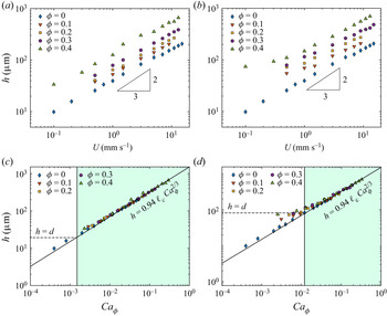
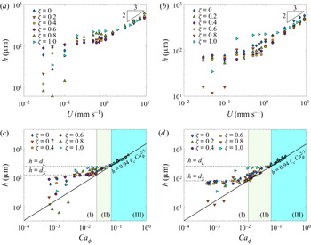
We measure the thickness of the coating film for the bidisperse suspension shown in figure 5 varying the withdrawal velocity and the volume ratio of large particles  $\zeta$. Figure 6(a) shows the thickness of the coating film as a function of the withdrawal velocity. In the regime of fast withdrawal (here
 $U \gtrsim 2\ {\rm mm}\ {\rm s}^{-1}$), monodisperse and bidisperse suspensions follow a common power law
 $h \propto U^{2/3}$. This observation suggests that an effective viscosity can also be extracted for a thick enough film of bidisperse suspension. We perform an analysis similar to the one used for the monodisperse suspensions in § 3 and fit the thickness
 $h$ to the LLD law (3.1), where the effective viscosity
 $\eta (\phi )$ is considered as a fitting parameter. The rescaling is shown in figure 6(c). It demonstrates that the coating film is in the effective viscosity regime, provided that the film is thicker than the diameter of the large particles,
 $h \geq d_{L}$.
Thickness of the coating film as a function of (a,b) the withdrawal velocity  $U$ and (c,d) the effective capillary number
 ${Ca}_\phi$ for bidisperse suspensions with particles of diameter (a–c)
 $d_{S} = 20\ \mathrm {\mu }{\rm m}$ and
 $d_{L} = 80\ \mathrm {\mu }{\rm m}$ (
 $\delta =4$); (b–d)
 $d_{S} = 20\ \mathrm {\mu }{\rm m}$ and
 $d_{L} = 140\ \mathrm {\mu }{\rm m}$ (
 $\delta =7$). The volume fraction is
 $\phi = 20\,\%$. In each figure, we vary the volume ratio of large particles
 $\zeta$ from
 $0$ to
 $1$. In (c) and (d) the two horizontal dashed lines respectively correspond to a coating film thickness equal to the particle diameters,
 $h=d_{S}$ and
 $h=d_{L}$. The continuous thick line is the LLD law, where the viscosity is considered as a fitting parameter. We observe three regimes: (I) is the regime where the film thickness is more or less constant and similar to
 $d_{S}$; (II) is the regime where the film is primarily composed of small particles, and the number of large particles depends on the withdrawal velocity; (III) is the thick-film regime where the coating film is thicker than the diameter of the large particles, and the composition of the coating film is similar to that of the bath. Inset pictures show the coating film in these three regimes. The size of the scale bars is
 $250\ \mathrm {\mu }\rm {m}$.

The situation is nevertheless more complex than for monodisperse suspensions. Indeed, the threshold to the effective viscosity regime seems to depend on the volume ratio of large particles  $\zeta$. For small
 $\zeta$ (for instance
 $\zeta =0.2$ in figure 6c) the thickness of the film follows fairly well the LLD law as soon as
 $h \geq d_{S}$. Indeed, small values of
 $\zeta$ mean that the volume of large particles is small compared with the volume of small particles. Therefore, the large particles do not contribute significantly to the viscosity of the suspension. Note that, although the prediction of the LLD law is reasonably good when
 $d_{S} < h < d_{L}$, the composition of the coating film is different from the composition of the suspension bath with a deficit in large particles, as we shall see in § 4.3. For large values of
 $\zeta$ (for instance,
 $\zeta =0.8$ or
 $0.9$ in figure 6c), the LLD law is recovered only for
 $h \geq d_{L}$. In this case, the large particles are the main contributor to the viscosity of the suspension. Thus, recovering the LLD law requires the coating film to be thick enough (
 $h \geq d_{L}$) so that it can allow most of the particles to be entrained in the film.
The same observation can be made with another combination of particle sizes: figure 6(b) shows the case of a suspension with  $d_{L}=140\ \mathrm {\mu }{\rm m}$ and
 $d_{S}=20\ \mathrm {\mu }{\rm m}$ particles. In this case, the effective viscosity regime following the LLD law is also recovered for
 $h\geq d_{L} = 140\ \mathrm {\mu }{\rm m}$ (figure 6d). Here, a similar evolution than the one reported in figures 6(a) and 6(c) is observed.
We also considered a larger volume fraction:  $\phi =40\,\%$ of
 $d_{L}=250\ \mathrm {\mu }{\rm m}/d_{S}=140\ \mathrm {\mu }{\rm m}$ (figure 7a) and
 $d_{L}=250\ \mathrm {\mu }{\rm m}/d_{S}=80\ \mathrm {\mu }{\rm m}$ (figure 7b). Again, the coating thickness
 $h$ follows the LLD law with an effective capillary number
 ${Ca}_\phi$, where the viscosity of the bidisperse suspension is still considered as a fitting parameter. A similar behaviour to the one reported for suspensions at
 $\phi =20\,\%$ is observed: the effective viscosity regime starts at
 $h \geq d_{L}$, and the transition from the heterogeneous film to the effective viscosity regime is smoother for small fraction of large particles
 $\zeta$ (figure 7(c,d). Besides, since the particles used here are larger than the ones used in the
 $\phi =20\,\%$ case, we are also able to see the liquid-only regime, where barely any particles are entrained. This regime is observed at small values of
 ${Ca}_\phi$, and thus small
 $h$ (data on the bottom left corner indicated as (I) in figure 7c,d).
Thickness of the coating film as a function of (a,b) the withdrawal velocity  $U$, and (c,d) the effective capillary number
 ${Ca}_\phi$ for bidisperse suspensions with particles of diameter (a–c)
 $d_{S} = 140\ \mathrm {\mu }{\rm m}$ and
 $d_{L} = 250\ \mathrm {\mu }{\rm m}$ (
 $\delta =1.786$); (b–d)
 $d_{S} = 80\ \mathrm {\mu }{\rm m}$ and
 $d_{L} = 250\ \mathrm {\mu }{\rm m}$ (
 $\delta =3.125$). The volume fraction is
 $\phi = 40\,\%$. In (c) and (d) the two horizontal dashed lines correspond to a coating film thickness equal to the particle diameters, respectively
 $h=d_{S}$ and
 $h=d_{L}$. The continuous thick line is the LLD law, where the viscosity is considered as a fitting parameter.

4.2.2. Effective viscosity of bidisperse suspensions
Although the LLD law is recovered for bidisperse suspensions when  $h\geq d_{L}$, figures 6(a,b) and 7(a,b) show that, for a given value of
 $U$ and
 $\phi$, a change in the volume ratio of large particles
 $\zeta$ leads to a change in the film thickness. This observation is consistent with the influence of the composition of the solid phase on the viscosity: a change in
 $\delta$ or
 $\zeta$ causes a change in viscosity, hence a change in film thickness (Shapiro & Probstein Reference Shapiro and Probstein1992; Gamonpilas et al. Reference Gamonpilas, Morris and Denn2016; Thiévenaz et al. Reference Thiévenaz, Rajesh and Sauret2021).
The effective viscosity  $\eta (\phi, \delta, \zeta )$ is obtained by fitting the experimental data to the LLD law in the effective viscosity regime. Figure 8(a) (respectively 8b) reports the relative viscosity
 $\eta _{r}=\eta /\eta _0$ as a function of the volume ratio of large particles
 $\zeta$ for the experiments presented in figures 6(c) and 6(d) (respectively figures 7c and 7d). In figure 8(a), the volume fraction in the bath is
 $\phi =20\,\%$ and the sizes of the particles are
 $20\ \mathrm {\mu }{\rm m}/80\ \mathrm {\mu }{\rm m}$ and
 $20\ \mathrm {\mu }{\rm m}/ 140\ \mathrm {\mu }{\rm m}$. In figure 8(b), the volume fraction in the bath is
 $\phi =40\,\%$ and the sizes of the particles are
 $140\ \mathrm {\mu }{\rm m}/250\ \mathrm {\mu }{\rm m}$ and
 $80\ \mathrm {\mu }{\rm m}/250\ \mathrm {\mu }{\rm m}$. Between the two monodisperse cases, the relative viscosity
 $\eta _{r}$ as a function of
 $\zeta$ shows a parabolic curve, reaching its minimum around
 $\zeta \simeq 0.4-0.6$. This canonical behaviour of bidisperse suspensions is due to the higher compacity of bidisperse packings (see e.g. Pednekar, Chun & Morris Reference Pednekar, Chun and Morris2018). The difference in viscosity observed between the two monodisperse cases, at
 $\zeta =0$ and
 $\zeta =1$, arises from the size variance of the particles. Although the suspensions used are monodisperse down to a certain level (see the size measurement in the Appendix), a small amount of polydispersity is unavoidable and, therefore, the maximum packing fraction for these two distributions of particles is slightly different of approximately
 $5\,\%-10\,\%$ here.
Relative shear viscosity  $\eta _{r}$ as a function of the volume fraction of large particles
 $\zeta$ for a suspension containing (a)
 $\phi =20\,\%$ for particle size ratio
 $\delta =4$ (blue) and
 $7$ (red) and using
 $\phi _{film}=17\,\%$ in the coating film; (b)
 $\phi =40\,\%$ for particle size ratio
 $\delta =1.786$ (blue)
 $3.125$ (red) and using
 $\phi _{film}=35.5\,\%$ in the coating film. The symbols show data obtained by the best fit to the LLD law. The lines show the viscosity predicted by the Maron–Pierce correlation (2.2) using the maximum packing fraction given by (4.3).

For a bidisperse suspension in the effective viscosity regime ( $h > d_{L}$), the proportions of small and large particles are expected to be similar in the film and in the bath. The evolution of the viscosity can be modelled by calculating the maximal packing fraction
 $\phi _{m}(\delta, \zeta )$ of a bidisperse sphere packing of the same composition and then substituting it into the Maron–Pierce correlation (2.2). To compute the maximal packing fraction, we adapt the model of Ouchiyama & Tanaka (Reference Ouchiyama and Tanaka1984). It consists in computing the local compacity around each size of particle and averaging it over the size distribution. The model is simplified to consider here a bimodal size distribution. The number fractions of small
 $N_{S}$ and large
 $N_{L}$ particles are defined as
 \begin{equation} N_{S} = \frac{(1-\zeta) \delta^3}{(1-\zeta) \delta^3 + \zeta} \quad {\rm and} \quad N_{L} = \frac{\zeta}{(1-\zeta) \delta^3} N_{S},\end{equation}
respectively, and  $\widetilde {d_{S}} = d_{S}/\delta$ and
 $\widetilde {d_{L}} = d_{L}/\delta$ are the reduced sizes given by
 \begin{equation} \widetilde{d_{S}} = \frac{(1-\zeta) \delta^3 + \zeta }{(1-\zeta) \delta^3 + \zeta\delta} \quad {\rm and} \quad \widetilde{d_{L}} = \delta \widetilde{d_{S}}.\end{equation}
The maximum packing fraction of the bidisperse packing is then given by
 \begin{equation} \phi_{m}(\delta,\zeta) = \frac{N_{S} \widetilde{d_{S}}^3 + N_{L} \widetilde{d_{L}}^3} {(N_{S}/\varGamma)(\widetilde{d_{S}}+1)^3 + N_{L} ( (\widetilde{d_{L}}-1)^3 + [(\widetilde{d_{L}}+1)^3 - (\widetilde{d_{L}}-1)^3 ]/\varGamma)}, \end{equation}
where  $\varGamma$ denotes the average number of particles in the vicinity of a given particle and is equal to
 \begin{align} \varGamma = 1 + \frac{4}{13} (8\phi_{m,0}-1) \frac{\displaystyle N_{S} (\widetilde{d_{S}} +1)^2 \left( 1 - \frac{3}{8} \frac{1}{\widetilde{d_{S}}+1} \right) + N_{L} (\widetilde{d_{L}}+1)^2 \left( 1 - \frac{3}{8} \frac{1}{\widetilde{d_{L}}+1} \right)}{N_{S} \widetilde{d_{S}}^3 + N_{L} [ \widetilde{d_{L}}^3 - (\widetilde{d_{L}}-1)^3]}.\end{align}
Here,  $\phi _{m,0}$ is the maximum solid fraction in a monodisperse packing, which we estimated through our rheometer measurements at
 $\phi _{m,0} \simeq 58\,\%$. We then compute
 $\phi _{m}$ using (4.3) and obtain the viscosity through the Maron–Pierce correlation given by (2.2). This approach has been previously used to describe the viscosity of a bidisperse suspension in an oscillating plane Couette flow (Gondret & Petit Reference Gondret and Petit1997), or the detachment of drops of bidisperse suspensions (Thiévenaz et al. Reference Thiévenaz, Rajesh and Sauret2021).
Figures 8(a) and 8(b) report the viscosity measured by fitting the dip-coating results to the LLD law, and comparing it with the predictions of (2.2) and (4.3). These predictions match our experiments well, proving that the bidisperse suspensions behave like an effective viscous fluid. Here, the volume fraction  $\phi$ is also determined by the best fit of the evolution of the viscosity with the composition of the bidisperse suspension. Achieving this good match requires that we use a volume fraction
 $\phi _{film}$ slightly smaller than the volume fraction in the suspension bath
 $\phi$ as
 $\phi _{film} \simeq 17\,\%$ for
 $\phi =20\,\%$ and
 $\phi _{film} \simeq 35.5\,\%$ for
 $\phi =40\,\%$. This discrepancy is consistent with the self-filtration effect (Kulkarni et al. Reference Kulkarni, Metzger and Morris2010) and the observations made in the previous section for monodisperse suspensions as there are fewer particles in the film than in the bath, regardless of their sizes.
The comparisons between the viscosity obtained from the LLD law and the model show that, at small size ratios ( $\delta = d_{L}/d_{S}$), the viscosity is well predicted over the whole range of
 $\zeta$. However, at larger values of
 $\delta$, the model usually fails for
 $\zeta >60\,\%$, i.e. when large particles dominate. This is explicit in figure 8(a). The same failure of the model has been observed in other configurations (Gondret & Petit Reference Gondret and Petit1997; Thiévenaz & Sauret Reference Thiévenaz and Sauret2021). Therefore, the mismatch between experimental results and the prediction originates from the limitation of the model for the viscosity given by (2.2) and (4.3) and not a problem specific to dip coating.
In summary, for a bidisperse suspension, the effective viscosity regime is observed for a coating thickness larger than the diameter of the largest particles  $h > d_{L}$. This condition can be expressed in terms of capillary number associated with the interstitial fluid
 \begin{equation} {{Ca}_0}^* \geq 1.09 \frac{\eta_0}{\eta(\phi,\delta,\zeta)} \left(\frac{d_{L}}{\ell_c}\right)^{3/2}, \quad {\rm with} \ {Ca}_0=\eta_0 U/\gamma, \end{equation}
or associated with the capillary number based on the effective viscosity of the bidisperse suspension
 \begin{equation} {{Ca}_\phi}^* \geq 1.09 \left(\frac{d_{L}}{\ell_c}\right)^{3/2}, \quad {\rm with} \ {Ca}_\phi=\frac{\eta(\phi,\delta,\zeta) U}{\gamma}. \end{equation}
This threshold is similar to the case of monodisperse suspensions (Gans et al. Reference Gans, Dressaire, Colnet, Saingier, Bazant and Sauret2019; Palma & Lhuissier Reference Palma and Lhuissier2019) but only depends on the diameter of the large particles. In the effective viscosity regime, the thickness of the coating film can be estimated using the LLD law with a capillary number based on the effective viscosity of the bidisperse suspension
 \begin{equation} h=0.94 \ell_c {{Ca}_\phi}^{2/3}. \end{equation}
For a given solid volume fraction, bidisperse suspensions are less viscous than monodisperse suspensions. This decrease in viscosity is more pronounced for a large difference in the particle size ratio, that is, when  $\delta$ is high (see figure 8a,b). Therefore, in the effective film regime, bidisperse suspensions yield thinner films than monodisperse suspensions for a given volume fraction
 $\phi$.
4.3. Heterogeneous regime
4.3.1. Experimental observations
For withdrawal velocities  $U$ leading to coating films thinner than the diameter of the large particles (
 $h \lesssim d_{L}$), the coating thickness does not follow the LLD law anymore. This situation is observed in regions (I) and (II) in figures 6(c,d) and 7(c,d). This heterogeneous regime, which was already observed for monodisperse suspensions, is different depending on the range of sizes of the particles. The heterogeneous regime can be split into two regimes for bidisperse suspensions.
The first regime corresponds to the lowest capillary numbers, where the film is then mainly composed of small particles. Its thickness remains more or less constant and equal to  $h \sim d_{S}$ over a range of capillary numbers (region (I) in figures 6c,d and 7c,d). A similar regime is observed for monodisperse suspensions and corresponds to a monolayer of small particles (Gans et al. Reference Gans, Dressaire, Colnet, Saingier, Bazant and Sauret2019; Palma & Lhuissier Reference Palma and Lhuissier2019). If the suspension is dilute enough and the particles are large enough, we can observe an extreme case where only the liquid is present in the coating film, without any entrained particles. This situation occurs at very small withdrawal velocities (left panel in figure 1). It can also be seen when the suspension is primarily composed of large particles (
 $\zeta =0.8$ in figure 7c,d).
The second heterogeneous regime occurs at moderate capillary number, between the first heterogeneous regime and the effective viscosity regime. In this regime, corresponding to region (II) in figures 6(c,d) and 7(c,d), the coating film is primarily composed of small particles but also contains some large particles. The number of entrained large particles increases continuously with the capillary number, up to the effective viscosity regime when  $h \geq d_{L}$. For a small volume ratio of large particles, typically
 $\zeta =0.2$ or
 $0.4$, the LLD regime is reached earlier than for large
 $\zeta$. This observation can be rationalized by considering that the number of large particles remains small. Therefore, the large particles do not contribute significantly to the effective viscosity of the suspension. The main challenge in predicting the threshold between the regimes lies in estimating the number of entrained particles. In the following subsection, we propose a filtration model that accounts, at first order, for the variation of the composition in the coating film.
4.3.2. Discussion: entrained particle distribution
When  $h< d_{L}$, the interplay between the different length scales (different sizes of particles and film thickness) selects the particles entrained in the coating film. We present here a model that accounts for the variation in the composition of the coating film compared with the composition of the bath. We rely on the thickness of the coating film and the flow rate based on the LLD theory of dip coating (Levich & Landau Reference Levich and Landau1942) to which we add the criterion given by (1.2), to set the minimum film thickness required for the entrainment of particles of diameter
 $d$ in the coating film. For a given particle size distribution in the bath, varying the withdrawal velocity and hence the thickness of the coating film will lead to a different particle size distribution in the coating film, as long as
 $h< d_{L}$.
Let us consider the passage of particles from the bath to the film. We introduce  $z$ as the coordinate parallel to the solid surface,
 $x$ as the coordinate perpendicular to the surface and
 $s$ is the curvilinear coordinate that follows the meniscus (see figure 2a). The lubrication flow in the film reduces to the axial flow profile
 $u_{z}^{*}(x, s)$. Then, the probability for a particle of diameter
 $d$ and position
 $(x, s)$ to be captured in the film is defined as
 $p_{c}^{*}(x, s, d)$. In addition, the particle–surface pair correlation function for a particle of diameter
 $d$ following a streamline passing through the point
 $(x, s)$ in the meniscus is defined as
 $g_{s}^{*}(x, s, d)$. This function describes the interaction between the surface and the particles. The equilibrium pair correlation may be needed to account for non-equilibrium effects of particles passing through the meniscus, for instance, the clustering of particles or interactions between them. From there, the flow rate of particles of diameter
 $d$ that enters the film,
 $Q_{c}(d)$, is computed. The local flux is first integrated over a cross-section of the meniscus, perpendicular to the plate and passing through the stagnation curve defined as
 $x = h^*(s)$
 $Q_{c}(d)$ can be expressed as
 \begin{equation} Q_{c}(d)=\phi(d) \oint \int_{0}^{h^{*}(s)} u_{z}^{*}(x, s) p_{c}^{*}(x, s, d) g_{s}^{*}(x, s, d) \,{\rm d} x \, {\rm d} s. \end{equation}
The general expression for the particle flow rate given by (4.8) allows us to account for complex solid surface geometries, such as fibres or textured plates (Dincau et al. Reference Dincau, Mai, Magdelaine, Lee, Bazant and Sauret2020; Seiwert et al. Reference Seiwert, Clanet and Quéré2011), and general particle–surface correlations. Here, we can make some assumptions for the sake of simplification by considering the cross-section of a thin plate so that the  $s$ dependence can be neglected during integration over the perimeter
 $P=2 (w+e)$, where
 $w$ and
 $e$ are the width and the thickness of the glass plate, respectively. A thin-film assumption is also made in Cartesian coordinates (
 $x$,
 $z$)
 \begin{equation} Q_{c}(d) = \phi(d) P \int_{0}^{h^{*}} u_{z}^{*}(x) p_{c}^{*}(x, d) g_{s}^{*}(x, d)\, {\rm d} x. \end{equation}
We further assume that a particle entering the meniscus is entrained if and only if its radius is smaller than the meniscus at the stagnation point (Sauret et al. Reference Sauret, Gans, Colnet, Saingier, Bazant and Dressaire2019), so that a capture probability function can be approximated as
 \begin{equation} p_{c}^{*}(x, d)=H\left(h^{*}-\frac{d}{2}-x\right), \end{equation}
where  $H(x)$ is the Heaviside step function. Note that other ansatze for
 $p_{c}^{*}(x, d)$ could be used to describe the entrainment of more complex particles (emulsion droplets, deformable capsules or anisotropic particles). We also assume the following expression for the particle–surface pair correlation function:
 \begin{equation} g_{s}^{*}(x, d) \approx \bar{g}_{s}^{*}(d) H(x-d/2), \end{equation}
where the Heaviside function takes into account excluded volume near the surface ( $x< d/2$), and the constant meniscus surface correlation
 $\bar {g}_{s}^{*}(d)$ reflects long-range particle–surface forces or dynamical effects, such as boundary layer depletion, that rescales the particle density arriving within the meniscus region relative to the well-mixed bulk fluid. In this approximation, the volume fraction of particles of diameter
 $d$ entering the meniscus region (outside the excluded volume near the wall) is
 $\phi ^{*}(d)=\bar {g}_{s}^{*}(d) \phi (d)$, which could be considered similar to the bulk volume fraction for a well-mixed suspension with
 $\bar {g}_{s}^{*}(d) \simeq 1$. Besides neglecting variations in particle mass transfer to the meniscus region, the following analysis also neglects interactions between particles that may lead to cooperative entrainment phenomena. For instance, a large particle can briefly deform the interface at the meniscus so that nearby smaller particles are more easily entrained. In particular, clusters of particles have been shown to be able to be collectively entrained at small film thickness (Colosqui et al. Reference Colosqui, Morris and Stone2013; Sauret et al. Reference Sauret, Gans, Colnet, Saingier, Bazant and Dressaire2019) and could, in principle, be accounted for through this function. In the following, we consider its simplest expression.
With these assumptions, (4.9) reduces to the integral over part of the velocity profile in the meniscus,
 \begin{equation} Q_{c}(d) = \phi^{*}(d) P \int_{d/2}^{h^{*}-d/2} u_{z}^{*}(x) \, {\rm d} x. \end{equation}
We further assume an approximately parabolic velocity profile vanishing at the stagnation point,
 \begin{equation} u_{z}^{*}(x) = U\left(1-\frac{x}{h^{*}}\right)^2. \end{equation}
This expression for the velocity field ensures the mass conservation for the case of a pure liquid going into the film,  $\int _{0}^{h^{*}} u_{z}^{*}(x)\,{\rm d} x=U h$. We substitute the flow profile given by (4.13) into (4.12) and perform the integral to obtain the probability distribution of particles in the coating film
 $\phi _{c}(d)$, defined as the volume fraction of particles of diameter
 $d$
 \begin{equation} \phi_{c}(d)=\frac{Q_{c}(d)}{Q_{f}}=\phi(d) f(\tilde{d}) H(1- \tilde{d}), \end{equation}
where  $\phi (d)$ is the probability distribution of particles in the suspension bath,
 $Q_{f}$ is the flow rate of liquid in the coating film and the Heaviside function
 $H(1- \tilde {d})$ indicates a sharp size cutoff given by entrainment criterion
 $\tilde {d}={d}/{2 h^{*}}<1$. In (4.14), the filtration function defining the ratio of final to initial probability distribution of particles is given by
 \begin{equation} f(\tilde{d})=(1-\tilde{d})^{3}-\tilde{d}^{3}, \end{equation}
where we have introduced a dimensionless particle radius as
 \begin{equation} \tilde{d}=\frac{d}{2 h^{*}}=\frac{d}{5.64 \ell_c {{Ca}_\phi}^{2 / 3}}. \end{equation}
Note that we have used here a thickness at the stagnation point calculated with the effective viscosity of the suspension. However, because of the similar size between the particles and the stagnation point, the local thickness may be modified by the volume fraction, and the size of the particles as described recently in the wetting dynamics by Zhao et al. (Reference Zhao, Oléron, Pelosse, Limat, Guazzelli and Roché2020). Further experiments focusing on the exact structure and local composition of the suspension at the meniscus would be needed to refine this assumption. The thickness in this region will be set by the deformation of the meniscus, the viscosity in the bath and the ratio of particle size to the typical length scale. This assumption could lead to small discrepancies in quantitatively estimating the number density of entrained particles. As expected,  $f(0)=1$, so that all particles that are small compared with the film thickness will be entrained if they arrive at the meniscus. The number of entrained particles of diameter
 $d$ per unit area in the coating film is thus given by
 \begin{equation} n_{p}(d)=\frac{Q_{c}(d)}{U P V_{p}(d)}=\frac{\phi_{c}(d) h}{V_{p}(d)}=\frac{\phi(d) f(\tilde{d}) H(1- \tilde{d}) h}{V_{p}(d)}, \end{equation}
where  $V_{p}(d)={\rm \pi} d^{3}/6$ is the volume of the spherical particle, and
 $h$ is the film thickness. The total entrained solid volume fraction and total solid flow rate (entrained volume per time) in the coating are expressed as
 \begin{equation} \phi_{p}=\int_{0}^{\infty} \phi_{c}(d)\,{{\rm d}} \,{d} \quad {\rm and} \quad Q_{s}=\int_{0}^{\infty} Q_{c}(d)\, {\rm d} \,{d}=\phi_{p} Q_{f}. \end{equation}
We apply these equations to the particular case of the bidisperse suspensions used in this study. We can express the probability distribution of small and large particles as  $\phi _{S}=(1-\zeta ) \phi$ and
 $\phi _{L}=\zeta \phi$, respectively. As a result, the number of small particles of radius
 $d_{S}$ entrained per unit area is
 \begin{equation} n_{p}(d_{S})=\frac{(1-\zeta) \phi f(\tilde{d}_{S}) H(1- \tilde{d}_{S}) h}{V_{p}(d_{S})}, \end{equation}
and for the large particles of diameter  $d_{L}$
 \begin{equation} n_{p}(d_{L})=\frac{\zeta \phi f(\tilde{d}_{L}) H(1- \tilde{d}_{L}) h}{V_{p}(d_{S})}. \end{equation}
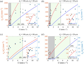
These expressions are plotted in figure 8(a–d) and show a fair agreement with the experimental data. The model yields quantitative results as it gives a reasonable estimate of the number of entrained particles when varying the volume ratio of large particles  $\zeta$ from
 $0.6$ (figure 8a) to
 $0.8$ (figure 8b). In both cases, the main limit occurs near the threshold velocity, where the model underpredicts the number of particles entrained. Indeed, the threshold for entrainment is based on the criterion for individual particles (Colosqui et al. Reference Colosqui, Morris and Stone2013; Sauret et al. Reference Sauret, Gans, Colnet, Saingier, Bazant and Dressaire2019), and does not account for the clustering of particles that deform the meniscus and allow particles at sufficient volume fraction to be entrained earlier. It was previously reported that the onset of the monolayer regime depends significantly on the volume fraction and so far remains empirically measured (Palma & Lhuissier Reference Palma and Lhuissier2019). Adding this component to the model presented above could lead to a better quantitative prediction of the density of entrained particles in this region. Nevertheless, the number density of particles is significantly filtered in this heterogeneous regime.
We have also performed similar measurements with smaller size differences ( $\delta =1.75$ in figure 8c). The experiments show that the velocity range in which particles could be separated by size is significantly reduced. In addition, figure 8(c) shows that, for similar particle sizes, a heterogeneous regime for both particle sizes is quickly reached and the prediction does not capture well the number of particles entrained per unit area. On the other hand, for large size difference (
 $\delta =12.5$ in figure 8d), there is a clear range below
 $U=2\ {\rm mm}\ {\rm s}^{-1}$ in which the film is free of large particles while entraining the small particles.
These results illustrate that, during the coating of a plate with a polydisperse suspension, the composition of the coating film may be very different compared with the composition of the bath. In the heterogeneous regime, the resulting coating will contain more small particles and fewer large particles than the original composition of the suspension, possibly compromising the quality of the coating.
We should emphasize that we have considered in our model a Heaviside step function in the capture probability function (4.10) and for the particle–surface pair correlation function (4.11). However, the transition between entrainment and no entrainment could be smoother. Considering the possible modification in our model, since  $u_{z}^{*}(x) = U(1-{x}/{h^{*}})^2$, smoothing the particle–surface interaction
 $g_{s}^{*}(x, d)$ will sample lower velocities (since
 $d/2$ is a hard sphere limit) and thus will lower the predicted entrainment fraction. Smoothing the capture function
 $p_{c}^{*}(x, d)$ could result in either of the following trends: (i) more probability weight at larger positions
 $x+d/2>h^*$, e.g. from particles that cooperatively ‘lift’ the meniscus to allow others to get into the film (Sauret et al. Reference Sauret, Gans, Colnet, Saingier, Bazant and Dressaire2019), will increase entrained volume fraction, and (ii) less weight at smaller sizes
 $x+d/2< h^*$ will lower it, e.g. from smaller particles that fluctuate across the stagnation point and are not entrained. If we assume that smoothing generally increases the effective diameter
 $d$ that can be entrained, then the present theory from (4.14) would predict more of the larger part of the initial distribution
 $\phi (d)$ gets past the cutoff function, i.e. more entrainment than predicted by a Heaviside function, as observed experimentally.
4.4. Using dip coating as a filtration method
The separation of small particles in the micron-size range (up to 1000  $\mathrm {\mu }$m) from a liquid dispersion is a source of challenge. When decreasing the particle size and increasing the batch volume, most filtering methods are neither very efficient nor suitable for a large throughput and/or are not highly selective. For example, the use of mechanical filters of specific pore size can quickly lead to clogging of the filter pores that slows down the filtering process (Urfer et al. Reference Urfer, Huck, Booth and Coffey1997; Wyss et al. Reference Wyss, Blair, Morris, Stone and Weitz2006; Sauret et al. Reference Sauret, Barney, Perro, Villermaux, Stone and Dressaire2014; Dressaire & Sauret Reference Dressaire and Sauret2017; Sauret et al. Reference Sauret, Somszor, Villermaux and Dressaire2018). Centrifugation is also a standard filtering method but cannot separate the particles with a high selectivity (Svarovsky Reference Svarovsky2000). Besides, centrifugation relies on the difference of density between the particles, and if the densities are comparable, the process loses in efficiency (Ninfa, Ballou & Benore Reference Ninfa, Ballou and Benore2009). However, a filtration method through a dip-coating process, as demonstrated in the insets of figure 9(a–d), depends on whether or not a particle enters in the coating film, which is mainly governed by the diameters of the particles and could therefore be used to sort particles by size, regardless of the particle volume fraction, as reported previously (Dincau et al. Reference Dincau, Bazant, Dressaire and Sauret2019). The main limitation to this method is that it is desirable to have particles with a significant size difference.
Number of particles deposited on a unit area of the plate. The composition of the suspension is (a)  $\phi =0.2$,
 $\zeta =0.6$,
 $\delta =7$ (
 $d_{S}=20\ \mathrm {\mu }{\rm m}$ and
 $d_{L}=140\ \mathrm {\mu }{\rm m}$); (b)
 $\phi =0.2$,
 $\zeta =0.8$,
 $\delta =7$ (
 $d_{S}=20\ \mathrm {\mu }{\rm m}$ and
 $d_{L}=140\ \mathrm {\mu }{\rm m}$); (c)
 $\phi =0.2$,
 $\zeta =0.9$,
 $\delta =1.75$ (
 $d_{S}=80\ \mathrm {\mu }{\rm m}$ and
 $d_{L}=140\ \mathrm {\mu }{\rm m}$); (d)
 $\phi =0.2$,
 $\zeta =0.9$,
 $\delta =12.5$ (
 $d_{S}=20\ \mathrm {\mu }{\rm m}$ and
 $d_{L}=250\ \mathrm {\mu }{\rm m}$). The blue and red symbols correspond to the experimental measurements for the large and small particles, respectively. The open squares represent the cases where the number of particles is underestimated because of limitations in the camera's depth of field and multi-layer deposition. The solid blue and red lines correspond to the theoretical predictions of the number of large (4.19) and small (4.20) particles per unit area on the plate, respectively. Insets: zoomed-in view on low withdrawal velocity region, highlighting the ability to filter the particles by size in the suspension.

The results demonstrated here with solid particles and a bimodal distribution could be extended to particles with a polydisperse size distribution and different material types. In addition, whereas the size of the entrained particles is limited here by the thickness of the liquid film, which is directly correlated to the capillary length, this filtration method could also be used with fibres (Dincau et al. Reference Dincau, Mai, Magdelaine, Lee, Bazant and Sauret2020). In this case, the thickness of the film, and thus the thickness at the stagnation point, is directly proportional to the radius of the fibre and therefore allows a larger range in size of particles that could be filtered.
In summary, the present methods offer various potential applications: in medicine, where it may be used to separate blood plasma components and cells (in a range of size from  $5$ to
 $50\ \mathrm {\mu }{\rm m}$), and for grains and powders, such as ceramic abrasives, where the standard methods of sedimentation or centrifugation are relatively slow, inaccurate and costly. Here, the possibility of scaling up the capillary filtering mechanisms with arrays of wires could open the opportunity for high throughput and good efficiency.
5. Conclusions
In this paper, we have investigated the dip coating of a plate withdrawn from a bath containing a suspension of particles with a bimodal size distribution. Previous studies have reported that different regimes are observed for monodisperse suspensions (Sauret et al. Reference Sauret, Gans, Colnet, Saingier, Bazant and Dressaire2019; Palma & Lhuissier Reference Palma and Lhuissier2019): no entrainment at low velocities; a heterogeneous regime with a monolayer of particles at intermediate velocity; and an effective viscosity regime when the film is thicker than the particle diameter. For bidisperse suspensions, the difference in diameter of the particles dispersed in the suspensions introduced a new complexity as additional length scales need to be compared with the film thickness. We have described the boundaries between the different coating regimes and shown that those transitions are dependent on withdrawal velocity (i.e. capillary number), volume fraction and composition of the suspensions. In particular, the bidispersity of the particulate suspensions led to a new regime at intermediate withdrawal velocity.
The behaviour observed for bidisperse suspensions is summarized in figure 1. At low velocity and moderate volume fraction, barely any particles are entrained. Increasing the withdrawal velocity leads to a peculiar behaviour: initially, only the small particles are entrained on the plate, and the coating exhibits a heterogeneous regime with a monolayer of small particles. Increasing the withdrawal velocity further leads to a second velocity threshold where the large particles start to be entrained. The number of entrained large particles gradually increases with the withdrawal velocity. Finally, at large enough withdrawal velocities, the composition of the suspension in the coating film is mostly similar to the composition of the suspension in the bath. A model that accounts for the probability of entraining particles based on their size has been developed. The model qualitatively reproduces the experimental measurements, although the heterogeneous regime where particles are entrained collectively is not captured in this model.
Our experiments have also revealed that the size of the largest particles in the suspension controls the onset of the effective viscosity regime. When the thickness of the coating film becomes larger than the diameter of the large particles,  $h \geq d_{L}$, the thickness can be predicted at first order by the LLD law by considering the effective viscosity of the bidisperse suspension. The presence of the different particle sizes, however, lowers the viscosity of the suspension for a given volume fraction
 $\phi$, and the evolution of the viscosity is well predicted by a model that considers the polydispersity and its influence on the maximum packing fraction. We should emphasize that both in the monodisperse and bidisperse regimes, the volume fraction of particles in the coating film always exhibits a slight decrease compared with the volume fraction in the liquid bath, likely due to a self-filtering mechanism that deserves further investigations.
As illustrated in this paper, the dip-coating process is not only an efficient tool to passively control the coating by tuning the thickness of the coating film, but can also be utilized as a method to sort particles by size in polydisperse suspensions. In particular, we have developed a model that predicts the resulting composition in particles of the coating film, knowing the probability distribution function of particles in the liquid bath and the withdrawal velocity of the substrate. The experiments reported here could also be used backwards in order to infer the capture function from the data using the theory, by solving an integral equation inverse problem. Such an approach would be particularly interesting to quantify different effects such as the shape, concentration or surface chemistry of the particles. We have also identified when an effective viscosity model for a polydisperse suspension could be used to predict the resulting coating thickness. The present contribution is a new step towards a predictive model to describe the formation of thin films with solid particulate suspensions. Nevertheless, further work is needed to capture the coating films formed with other types of suspensions, such as fibres or emulsion droplets.
Acknowledgements
The authors thank collaborators at Saint-Gobain Research North America, and in particular Y. Tian, J. Alex Lee and C. Li.
Funding
This material is based upon work supported by the National Science Foundation under NSF CAREER Program Award CBET Grant No. 1944844.
Declaration of interests
The authors report no conflict of interest.
Author contributions
D.H.J.: Methodology, investigation, formal analysis, data curation, visualization, writing – original draft; M.K.H.L.: investigation, writing – review and editing; V.T.: methodology, writing – review and editing; MZB: conceptualization, methodology, writing – review and editing; A.S.: conceptualization, methodology, supervision, writing – review and editing, funding acquisition, project administration.
Appendix. Physical properties of the polystyrene particles
The particulate suspensions used in this study consist of spherical polystyrene particles (Dynoseeds TS, Microbeads) dispersed in silicone oil (AP100, Sigma Aldrich). Particles with four different sizes have been used. We have measured the size distribution of each batch of the particles. Pictures of a large number of particles are taken and processed through ImageJ to obtain the projected area  $A$ of each particle. The diameter of the particles
 $d$ was then obtained from the project area,
 $d=2\sqrt {A/{\rm \pi} }$, considering that the circularity of the particles is close to 1. The measured size and standard deviation of each batch of particles are reported in table 1. The probability density function of the size distribution is plotted and fitted with a Gaussian distribution curve in figure 10.
Mean diameter and density of the polystyrene particles used in this study.

Probability density function (PDF) of diameter of the polystyrene particles used in this study and corresponding Gaussian fits.

The density of the particles was measured by mixing a batch of particles into salt water with known densities. The density of each batch of particles is also reported in table 1.