2.1 Electron cryo-microscopy (cryo-EM)

One of the main areas for the application of direct electronic detectors in the future is likely to be in the structural analysis of biological molecules using cryo-EM. Structural information to near-atomic resolution is needed to understand detailed molecular mechanisms in biological molecules, which is a prerequisite to understand their functionality. The structural integrity of biological molecules is very quickly destroyed by exposure to an electron beam and so imaging of high-resolution structural information must be done with very limited dose. In cryo-EM, samples are held in a thin amorphous film of ice and kept at cryogenic temperatures. The use of low temperatures inhibits the movement of the by-products of radiolysis and for the resolutions of interest in biology this allows a 5- to 10-fold increase, relative to room temperature, in the useable electron dose. Despite this increase, the number of electrons that can be used is still restricted to ~20 electrons/Ų (Baker & Henderson, Reference Baker and Henderson2002) and this severely restricts the signal-to-noise ratio that can be obtained in high-resolution images. As the signal-to-noise ratio of the images cannot be improved by increasing the number of electrons, improving the detector's performance is crucial in order to realize the full potential of cryo-EM.

Cryo-EM is a powerful technique that allows not just the static but also dynamic studies of intermediate states in macromolecular interactions by recording trapped states (Subramaniam et al. Reference Subramaniam, Lindahl, Bullough, Faruqi, Tittor, Oeterhelt, Brown, Lanyi and Henderson1999; Frank, Reference Frank2002). Although the resolution obtained with cryo-EM is usually currently somewhat lower than that for X-ray crystallography, the two techniques are increasingly being used in tandem: with spatial co-ordinates provided by high-resolution structures obtained with X-ray crystallography being docked with lower-resolution cryo-EM structures. Any structural changes induced by, for example, ligand-binding, can then be studied by using cryo-EM without the need to re-crystallize the modified macromolecule. Large macromolecular complexes, which are difficult to study by single-crystal analysis, have been solved by combining the individual crystal structures of individual, smaller components of the large complex and fitted in a lower-resolution EM map (Frank, Reference Frank2002).

Three of the most commonly employed techniques for structure determination, within the general field of cryo-EM, are described very briefly below; they include single-particle reconstruction, electron crystallography and electron tomography.

2.2 Low-energy electron microscopy (LEEM)/photo-emission electron microscopy (PEEM)

LEEM is a relatively new technique, which has been extremely useful for studying the topography of surfaces (Bauer, Reference Bauer1994; http://www.leem-user.com/). The static or dynamic structure of surfaces is investigated at sub-micrometer resolution (in favourable cases a resolution of ~50 Å is possible) by using ‘reflected’ low-energy electrons (0–100 eV) from the surface as probes. Due to the large back-scattering cross-sections at such low energies, it is possible to obtain large signals and hence good contrast (Tromp, Reference Tromp2000; Bauer, Reference Bauer2009). Contrast is obtained by surface topography and variations in work function. EM at such low energies is made possible by using specialized electron optics to decelerate electrons from ~20 keV to under 100 eV for the imaging process. Subsequently, the backscattered electrons are accelerated up to ~20 keV, where the images are recorded. Additionally, samples can be illuminated with ultra-violet light causing photoemission of low-energy electrons in a complementary technique called photo-emission electron microscopy (PEEM), which provides similar information to LEEM.

Traditionally, LEEM/PEEM images have been recorded on detectors based on microchannel plates (MCP) coupled to light-sensitive CCDs; limitations of these detectors include restricted dynamic range, noise in images due to readout and poor spatial resolution. Improvements in recording images can be made by using direct detection in pixel detectors, based on CMOS (Deptuch, Reference Deptuch2005; Matheson et al. Reference Matheson, Moldovan, Clark, Prydderch, Turchetta, Derbyshire, Kirkland and Allinson2009) or Medipix2 (van Gastel et al. Reference Van Gastel, Sikharulidze, Schramm, Abrahams, Poelsema, Tromp and Van Der Molen2009) with similar advantages as already mentioned for the electrons with higher energies used for TEM, and reviewed in Faruqi (Reference Faruqi2009).

The first type of pixel detector, viz. MAPS, has been evaluated by Matheson et al. (Reference Matheson, Moldovan, Clark, Prydderch, Turchetta, Derbyshire, Kirkland and Allinson2009) for use in low-energy electron detection ranging from 10 to 20 keV. The detector, called Vanilla, was developed within the MI3 collaboration (MI3; http://mi3.shef.ac.uk/) for various applications, including the fast readout mentioned in Section 4.3.4 used for single-electron image processing (McMullan et al. Reference McMullan, Clark, Turchetta and Faruqi2009b). The Vanilla detector contains 520×520 25 μm pixels with an epilayer thickness of either 16 or 20 μm. Front-illuminated MAPS are not suitable for low-energy electron detection as normal chip design includes the deposition of a layer of material (consisting of an overall passivation layer and multiple polysilicon and metallic layers) on top of the sensitive epilayer and through which low-energy electrons cannot penetrate. The solution for low-energy electron detection is to back-illuminate the sensor (Deptuch, Reference Deptuch2005; Cabello et al. Reference Cabello, Bailey, Kitchen, Prydderch, Clark, Turchetta and Wells2007; Deptuch et al. Reference Deptuch, Besson, Rehak, Szelezniak, Wall, Winter and Zhu2007); this is achieved by back-thinning of the substrate material to such an extent that there is little or no residual material between the entry point for the electron and the epilayer (Fig. 9 in Section 4.3 shows a typical layout of a MAPS pixel) (Cabello & Wells, Reference Cabello and Wells2007; Cabello et al. Reference Cabello, Bailey, Kitchen, Prydderch, Clark, Turchetta and Wells2007). A further advantage of this configuration is that with a sufficiently thick epilayer the incident electrons cannot reach the radiation-sensitive oxide layers on the other side of the epilayer and so there is little direct radiation damage. At 20 keV, the spatial resolution and DQE of the MAPS detectors were found to be significantly better than currently used MCP detectors (Matheson et al. Reference Matheson, Moldovan, Clark, Prydderch, Turchetta, Derbyshire, Kirkland and Allinson2009). However, with decreasing energy, the performance of the MAPS detector deteriorated relative to that of the MCP. This was put down to the thickness of the residual dead layer on the epilayer after back-thinning and it is believed that the drop in performance can be removed through the use of a more state-of-the-art surface processing.

van Gastel et al. (Reference Van Gastel, Sikharulidze, Schramm, Abrahams, Poelsema, Tromp and Van Der Molen2009) have evaluated the relative performance of Medipix2 hybrid pixel detector with MCP detectors for use in LEEM/PEEM. The applied bias and negligible stopping power of the coating on the surface of the silicon sensor in Medipix2 make it unnecessary to perform any additionally back-thinning steps as are needed with the MAPS detector. Medipix2 allows high count rates, noiseless readout (provided the pixel threshold is set above the noise limit) and unlimited dynamic range provided multiple images are summed; further, as electrons are stopped well within the 300-μm-thick sensor, there is no problem of radiation damage (Mettivier et al. Reference Mettivier, Montesi and Russo2004; Faruqi et al. Reference Faruqi, Henderson and Tlustos2005b) over extended usage. The authors conducted a series of tests comparing the performance of Medipix2 with the Chevron 3040FM MCP detector installed on an Elmitec LEEM III instrument (http://www.elmitec-gmbh.com/). It was found that the spatial resolution in Medipix2 was better by about a factor of 3 at ~20 keV. The main conclusion from both studies was that direct electron detection in back-illuminated MAPS or in Medipix2 offers significant advantages over detectors based on MCP coupled to CCDs.

2.3 Ultrafast EM

Time-resolved studies of structural changes provide valuable information on dynamic phenomena both in the biological and physical sciences. Transient events, which occur on a rapid timescale, have been studied in pump–probe experiments combined with EM (King et al. Reference King, Campbell, Frank, Reed, Schmerge, Siwick, Stuart and Weber2005; Zewail, Reference Zewail2006; Park et al. Reference Park, Baskin, Barwick, Kwon and Zewail2009). The method generally relies on a photo-activated electron gun that is gated by a laser pulse for a very short time period – typically nanoseconds. A high DQE detector is clearly an important requirement for this method. The choice of detector would be dependent on the electron energies used for imaging; as described earlier, for energies up to ~120 keV, Medipix2 would offer particular advantages over CCDs due to the higher DQE. At electron energies >120 keV, a MAPS detector would offer similar advantages as discussed in Section 4.3.

3.1 Resolution and efficiency

Optimization of the imaging detector performance is important in many areas of EM. It is vital in the study of radiation sensitive samples where only a small electron dose can be used to generate an image. However, it is also valuable in the study of more radiation-resistant samples as it allows exposure times to be reduced (King et al. Reference King, Campbell, Frank, Reed, Schmerge, Siwick, Stuart and Weber2005). The characterization of an imaging detector requires evaluation of its performance as a function of spatial frequency. Since the magnification of the microscope can be varied, it is the response relative to the detectors pixel size, rather than of the sample that is important. Current detectors consist of a regular 2D array of pixels and so spatial frequency is naturally described using the components of the discrete Fourier transform. As different detectors can have different pixel counts, it is convenient to measure the spatial frequency, ω, relative to the Nyquist frequency given by the reciprocal of twice the pixel spacing.

The resolution of a detector is given by the MTF, which describes the variation in the ratio of output to input amplitude as a function of spatial frequency. In an electron microscope, it is most conveniently measured using the knife-edge method (Dainty & Shaw, Reference Dainty and Shaw1974; McMullan et al. Reference McMullan, Chen, Henderson and Faruqi2009a). The response of a pixellated detector is proportional to the integral of the signal in a pixel and this leads to decay in the MTF as sin(πω/2)/(πω/2). The MTF is further degraded by the point spread function of the response in the detector to an incident electron. The point spread function is proportional to the average response as a function of distance from the incident position on the detector of an electron. It does not depend on whether the response comes from summing many different stochastic contributions or is simply associated with a blurring that is essentially the same for each incident electron. It useful to have a high MTF over all spatial frequencies, but for radiation-tolerant samples any fall in MTF with increasing spatial frequency can be compensated for by simply using a higher magnification, albeit with a loss in field of view.

While the MTF describes what the amplitude of a signal will be as a function of spatial frequency the DQE measures how strong the signal will be relative to the noise. In the study of radiation-sensitive samples, the DQE is important as the limited electron dose that can be used leads to images in which any signal is barely above the associated shot noise. The DQE was originally introduced at zero spatial frequency and defined as the ratio of the square of the signal-to–noise ratio out to that of the square of the signal-to–noise ratio in Zweig (Reference Zweig1965), Hamilton & Marchant (Reference Hamilton and Marchant1967) and Dainty & Shaw (Reference Dainty and Shaw1974). Electrons arrive at a detector as independent random events and so in an image with an average of n electrons per pixel there will be shot noise of in the input. The output noise, N _out, contains an amplified version of the input noise as well as contributions from both variation in the gain experienced by individual electrons and any additional readout so that

(3.1)

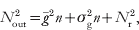
in which is the average gain, is the variance in the gain and N_r is the readout noise. Using this and the definition of DQE(0) gives

(3.2)

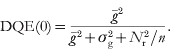
A perfect detector records all electrons equally (so that ) and has no readout noise (N _r=0), and consequently a DQE(0) of 1. Any variation in the response to individual electrons or additional readout noise will degrade the DQE.

To determine the DQE(0) of a real detector, the number of electrons per pixel, n, the average response, , and the output noise N _out, must be measured and together these give

(3.3)

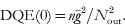
As the signal in one pixel can spill into adjacent pixels, is not simply the variance in the pixels but also includes correlation terms with neighbouring pixels. N _out can be estimated from the variation in the calculated variance as a function of pixel binning as described in McMullan et al. (Reference McMullan, Chen, Henderson and Faruqi2009a). The assumption being that for large pixel binning the boundary contributions will be negligible and the measured variance of the binned pixel arises from the sum of the individual contributions in the un-binned pixels. Alternatively, can be calculated directly as the sum of the inter pixel correlation function, i.e.,

(3.4)

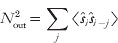
in which is the deviation from the mean output measured in the jth pixel and 〈K〉 indicates an average over all pixels.

The extension of the definition of DQE to finite spatial frequencies follows from: noting that via the Wiener–Kitichinne theorem, equation (3.4) can be recognized as the zero spatial frequency Fourier component of the noise power spectra, NPS(ω); by definition S _out/S _in is given by ; and the noise power spectrum associated with an average of n independent random electrons arriving on each pixel is constant and equal to n for each discrete Fourier component. Together these give

(3.5)

To obtain a high DQE over all spatial frequencies, it is helpful to have a high MTF(ω). However, in finitely sampled systems NPS(ω) includes aliased terms and the magnitude of these increases with the MTF(ω). As mentioned above, the MTF does not differentiate between whether the shape of the associated point spread function results from the summation of many different stochastic contributions or is associated with a blurring having essentially the same effect for each incident electron. With the NPS the difference has a big effect and leads to an important difference in the behaviour of the DQE with increasing spatial frequency between CCD and MAPS detectors. In a CCD, the MTF is degraded by the stochastic scattering of incident electrons in the phosphor and support matrix (Meyer & Kirkland, Reference Meyer and Kirkland1998). This leads to a decrease in the MTF that is not reflected in an associated decrease in the NPS. As a result a low MTF in a CCD detector is always reflected in a low DQE. For a MAPS detector, in particular one that is back-thinned beyond 50 μm, a major contribution to the decrease in MTF with spatial frequency results from charge diffusion in the sensitive epitaxial layer. The diffusion tends to affect the response in all electrons equally so that the associated reduction in MTF is reflected in a reduced NPS. Consequently, the fall in the MTF is not so strongly reflected in the DQE and it is possible to have an MAPS detector with what seems a poor MTF and yet having a high DQE. Moreover, as discussed in McMullan et al. (Reference McMullan, Chen, Henderson and Faruqi2009a), the fall-off in the MTF with increasing spatial frequency reduces the aliased contributions in the NPS and so enhances the DQE at higher spatial frequencies.

3.2 Field of view covered by the detector

Since the magnification in the electron microscope can be varied using the magnetic lenses, the area covered by the detector is less important, within space constraints, than the number of independent pixels available for recording images. The effective field of view of a detector is ultimately determined by its MTF(ω), but in practice the limit is set by the need to resolve signals above the noise, and hence the DQE(ω). Choosing a lower threshold for DQE(ω) results in an effective pixel size and hence the usable field of view. As mentioned in the introduction, at 300 keV, film can provide as many as 10k×10k independent pixels in an image, which is difficult to match in currently available electronic detectors. Two recently released indirect electron detector systems: the TemCam-F816 from TVIPS (http://www.tvips.com/Prod_TF816.php) with 8192×8192 pixels and the UltraScan 10 000XP from Gatan (http://www.gatan.com/contact/) with 10 560×10 560 pixels, seemingly offer a similar number of pixels to film but in practice at 300 keV they would have to be binned at least by a factor of 2 in order to match the performance of film.

3.3 Radiation damage

Radiation damage in the detector itself, as opposed to the specimen, is an important matter when electrons are detected directly. Residual charge generation, especially in oxide layers, and knock-on damage to crystal structure can quickly destroy the properties of electronic components. For this reason, direct electron detection using CCDs is not practical (Roberts et al. Reference Roberts, Chapman and Macleod1982) and instead electrons are detected via the light they generate in a phosphor. The phosphor and optical coupling shield the CCD from the direct electron beam. Radiation damage to the phosphor and its support matrix is much less severe and leads to small changes in the sensitivity that can be corrected for by refreshing the gain correction of the detector. With careful design, the radiation damage to CMOS devices can be minimized so that they can withstand many Mrads of radiation (Campbell et al. Reference Campbell, Anelli, Cantatore, Faccio, Heijne, Jarron, Santiard, Snoeys and Wyllie2001; Eid et al. Reference Eid, Chan, Fossurn, Tsai, Spagnuolo, Deily, Byers and Peden2001; Bogaerts et al. Reference Bogaerts, Dierckx, Meynants and Uwaerts2003; Faruqi et al. Reference Faruqi, Henderson and Holmes2006). This level of radiation tolerance is not sufficient for diffraction or high-dose experiments, but is sufficient to enable over one year of careful low-dose usage. The radiation damage in CMOS detectors chiefly manifests itself in an increase in ‘dark’ current (Faruqi et al. Reference Faruqi, Henderson, Prydderch, Turchetta, Allport and Evans2005a). The effects of this can be minimized by using faster readout and correcting using dark field images taken immediately before and after a ‘signal’ image.

3.4 Uniformity of response

Most detectors show some non-uniformity in pixel-to-pixel sensitivity. This can arise from many different contributions such as variability in the starting materials and their preparation, variation in detector layout, readout timing issues and radiation damage. Provided that the non-uniformities in the detector response are not too great, they are usually corrected for by a combination of ‘dark’ field and gain correction (derived from flood-field images illuminated with a uniform beam). The presence of a few dead or unusually noisy pixels, can also be corrected for by masking out these pixels and replacing them with the averages of their neighbours.

Ideally the response of a detector should also be linear with respect to electron dose. The range over which the response must be linear depends on the application. Low-dose cryo-EM images have very little contrast and so a detector such as a film is adequate. On the other hand, diffraction experiments require a much higher dynamic range that is more suited to CCD detectors. Electronic detectors with low noise and a fast readout can also be used to obtain a high dynamic range by summing multiple frames (McMullan & Faruqi, Reference McMullan and Faruqi2008).

3.5 Readout speed

The stroboscopic experiments described in Section 2.3 require detectors with a fast readout. Moreover, there are other experiments where fast readout speeds are either essential or extremely desirable. For example, high-resolution imaging requires considerable stability in the specimen position as any movement during imaging will degrade the resolution. With fast readout sample drift due to the stage can be removed by alignment of the individual images in an exposure consisting of a series of images. Taking exposures as a series of images has other advantages such as giving both high- and low-dose information in the same exposure and thereby allowing better determination of the defocus and optimal resolution-dependent exposures to be made. Fast readout is also very valuable in diagnostic experiments. For example, it was hoped that the image degradation due to specimen movement associated with charging and radiation damage could be minimized using stroboscopic imaging. An example of this is the loss in contrast observed in images of paraffin crystals relative to what is measured with diffraction (Henderson & Glaeser, Reference Henderson and Glaeser1985). Based on the assumption that beam-induced movements would have a ‘threshold’, i.e. would disappear at sufficiently small doses, there have been several attempts to considerably reduce the electron dose per frame during imaging. Typke et al. (Reference Typke, Gilpin, Downing and Glaeser2007) have used a stroboscopic imaging technique that reduces the electron dose per frame by about 30 times compared to normal imaging. The sub-images were summed, but only after an appropriate image shift had been applied to each frame, equivalent to the movement in that period. Despite the very low electron dose per frame, the authors did not obtain any improvement in image contrast. Glaeser et al. (Reference Glaeser, McMullan, Faruqi and Henderson2011) have used the Medipix2 detector, described in more detail in the next section, to further reduce the electron dose in sub-frames to ~500 electrons/frame, equivalent to 0·003/Ų. Using the noiseless readout of Medipix2 the authors assembled a time-sliced series of images from the same area of the specimen to obtain a ‘movie’ with up to 400 frames. Despite the very small dose of electrons per frame, image blurring was still observed; the original publication should be consulted for full experimental details, further associated experiments that were more successful and the conclusions that can be drawn.

4.1 CCDs

The earliest electronic detectors used for EM were based on low-noise readout ‘scientific grade CCDs’, originally developed for applications in optical astronomy and have been described in a number of reports and reviews (Krivanek & Mooney, Reference Krivanek and Mooney1993; Deruijter, Reference Deruijter1995; Meyer & Kirkland, Reference Meyer and Kirkland1998; Faruqi & Subramaniam, Reference Faruqi and Subramaniam2000; Janesick & Putnam, Reference Janesick and Putnam2003; Mooney, Reference Mooney2007). Due largely to radiation damage when used in direct detection mode (Roberts et al. Reference Roberts, Chapman and Macleod1982), CCD detectors for EM have been used with a phosphor–fibre-optics front end (Krivanek & Mooney, Reference Krivanek and Mooney1993; Spence & Zuo, Reference Spence and Zuo1988; Faruqi & Subramaniam, Reference Faruqi and Subramaniam2000) or in some cases with lens coupling (Fan & Ellisman, Reference Fan and Ellisman1993). Energy lost by electrons in the phosphor is converted into visible light, which is then imaged by the CCD. Spatial resolution suffers as a consequence of light scattering within the phosphor and fibre optics (Faruqi & Andrews, Reference Faruqi and Andrews1997). Despite this shortcoming, CCD detectors have been very usefully employed in a number of applications involving electron diffraction and lower-resolution imaging of single molecules in cryo-EM (Downing & Hendrickson, Reference Downing and Hendrickson1999; Faruqi et al. Reference Faruqi, Henderson and Subramaniam1999; Subramaniam et al. Reference Subramaniam, Lindahl, Bullough, Faruqi, Tittor, Oeterhelt, Brown, Lanyi and Henderson1999; Sander et al. Reference Sander, Golas and Stark2005; Booth et al. Reference Booth, Joanita and Chiu2006). The spatial resolution for CCD detectors is limited by the spread of light in the phosphor, the fibre-optics and at the fibre-optics–CCD interface (Faruqi & Andrews, Reference Faruqi and Andrews1997) and also the scattering of incident electrons in the phosphor and its support matrix (Meyer & Kirkland, Reference Meyer and Kirkland1998). The degradation of resolution and consequently DQE is particularly serious at higher energies and spatial frequencies.

4.2 Hybrid pixel detectors: Medipix2

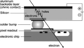
Hybrid pixel detectors were originally developed for infrared astronomy and charged particle detection (Shapiro et al. Reference Shapiro, Dunwoodie, Arens, Garrett Jernigan and Gaalema1989) and subsequently for particle physics at CERN (Campbell et al. Reference Campbell, Heijne, Jarron, Krummenacher, Enz, Declercq, Vittoz and Viertel1990). The technology was considered ideal for medical imaging and was further adapted for this and other types of X-ray imaging applications within the Medipix collaboration based at CERN (http://medipix.web.cern.ch/MEDIPIX; Da Via et al. Reference Da Via, Bates, Bertolucci, Bottigli, Campbell, Chesi, Conti, D'Auria, Delpapa, Fantacci, Grossi, Heijne, Mancini, Middelkamp, Raine, Russo, O'Shea, Scharfetter, Smith, Snoeys and Stefanini1997; Llopart et al. Reference Llopart, Campbell, Dinapoli, San Secundo and Pernigotti2002; Llopart & Campbell, Reference Llopart and Campbell2003; Mikulec et al. Reference Mikulec, Campbell, Heijne, Llopart and Tlustos2003; Mettivier et al. Reference Mettivier, Montesi and Russo2004); with minor modifications Medipix1 (Faruqi et al. Reference Faruqi, Cattermole, Henderson, Mikulec and Raeburn2003), and later Medipix2, were evaluated for use in EM over a range of electron energies (Faruqi et al. Reference Faruqi, Henderson and Tlustos2005b; McMullan et al. Reference McMullan, Cattermole, Chen, Henderson, Llopart, Summerfield, Tlustos and Faruqi2007). Medipix2 consists of a 300-μm-thick pixellated silicon sensor, which is operated in fully depleted mode via an applied bias voltage across the sensor. The sensor is bump-bonded to a readout application specific integrated circuit (ASIC) as shown in Fig. 1, which has an identical pixellation to the sensor. The bump bond provides each sensor pixel with a direct connection to a readout pixel on the ASIC. Each pixel has a complete readout electronics consisting of an amplifier, discriminator and a counter, in which count rates of up to ~1 MHz are possible. Incident electrons are detected by recording the charge due to the electrons or holes created in the silicon sensor. Electrons and holes are swept in opposite directions by a bias voltage applied across the sensor; holes are collected at the cathode, which is connected to the pixel amplifier in the electronics chip via the bump bond. The resultant signal, after amplification, results in a count if the signal is above a preset threshold. Counts in the whole array are accumulated over the preset exposure period and used to form the final image.

Fig. 1.

Schematic diagram of a single pixel of Medipix2, a hybrid pixel detector, developed within the Medipix collaboration (http://medipix.web.cern.ch/MEDIPIX). The sensor is fully depleted by an applied potential, with the polarity chosen to force holes to the readout electronics via the bump bond, as shown above. The incoming electron, which is to be detected, is shown as traversing the sensor and the readout chip. The figure is only a convenient representation of reality as electrons with energy below ~250 keV would be stopped within the 300 μm of silicon sensor material.

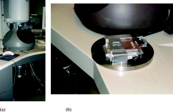
A general view of the Tecnai F30 transmission electron microscope is shown in Fig. 2a; the cylindrical vessel below the viewing chamber contains the Medipix2 detector. A photograph of a Medipix2 Quad detector in a special mounting plate is shown in Fig. 2b, prior to being attached to the microscope. An excellent basic description of the electron optics used in electron microscopes for non-specialists can be found in Slayter & Slayter (Reference Slayter and Slayter1992).

Fig. 2.

(a) A view of the F30 Tecnai Electron Microscope (FEI; http://www.fei.com/) with the Medipix2 detector, situated within a cylindrical container, mounted below the viewing chamber. (b) A Medipix2 detector prior to installation in the electron microscope. Due to the danger from secondary radiation, the base plate, on which the detector is mounted, is made from stainless steel. The detector face is covered with a square metal mask (with a cut out to allow electrons to be transmitted to the detector) to prevent electrons from damaging the electronics components on the detector periphery and readout electronics.

A detailed characterization of Medipix2, in Quad form (2×2 array), was carried out at the Laboratory of Molecular Biology (LMB) to investigate the suitability of the detector for EM at energies between 40 and 300 keV with more detailed studies at 120 keV. Experimental data obtained at 120 keV were compared with predictions from Monte Carlo simulations and excellent agreement was found (McMullan et al. Reference McMullan, Cattermole, Chen, Henderson, Llopart, Summerfield, Tlustos and Faruqi2007). The technology, which underpins Medipix2, along with numerous applications in many different fields and a comprehensive bibliography, has been published recently by Campbell (Reference Campbell2010).

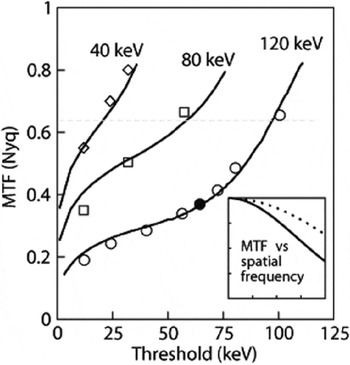
The MTF(ω) of the Medipix2 was characterized in terms of spatial resolution as a function of spatial frequency at energies of 40, 80 and 120 keV using the conventional knife-edge method (Dainty & Shaw, Reference Dainty and Shaw1974; McMullan et al. Reference McMullan, Cattermole, Chen, Henderson, Llopart, Summerfield, Tlustos and Faruqi2007). Global and individual pixel thresholds were varied to optimize the detector performance, in terms of flat-field response, spatial resolution and efficiency, for a given incident electron energy (Faruqi et al. Reference Faruqi, Henderson and Tlustos2005b; McMullan et al. Reference McMullan, Cattermole, Chen, Henderson, Llopart, Summerfield, Tlustos and Faruqi2007). A higher threshold setting results in fewer counts at a given energy; in an extreme case, with a threshold setting equivalent to 120 keV, there would be no counts in the pixel for a 120 keV incident electron even if the entire energy were to be deposited in a single pixel. A lower threshold results in more of the incident electrons being counted and also allows electrons to be recorded in multiple pixels, and if set too low results in erroneous noise counts. A compromise is needed in the threshold setting to optimize resolution without reducing the efficiency excessively. The effects of the threshold setting are discussed in more detail in McMullan et al. (Reference McMullan, Cattermole, Chen, Henderson, Llopart, Summerfield, Tlustos and Faruqi2007).

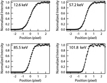
The edge functions, obtained at different values of the pixel thresholds, were used for obtaining the MTF curves at 40, 80 and 120 keV. The edge function, from which the MTF can be calculated, is defined as

where f(x) is the value of the average intensity at distance x from the edge, b is the bright value, i.e. not obscured by the opaque object and d is the dark value, i.e. obscured by the opaque object. The edge functions measured at 120 keV with the thresholds corresponding to energies of 12·2, 56·4, 80·5 and 100·6 keV are shown in Fig. 3. The slope of the edge function increases (becomes steeper) with increasing threshold – leading to a narrower point spread function and an improved MTF, as discussed in McMullan et al. (Reference McMullan, Cattermole, Chen, Henderson, Llopart, Summerfield, Tlustos and Faruqi2007). The experimental values of MTF at the Nyquist frequency as a function of threshold are shown as data points along with the continuous curves obtained from simulations, in Fig. 4. As shown in the figure, experimental data and simulations show excellent agreement. The horizontal dotted line is drawn at a value of 2/π, which represents the maximum possible value of MTF at the Nyquist frequency for a pixellated detector. This value is exceeded at higher thresholds due to the effective reduction in the pixel size as only electrons that effectively stay in the middle of a pixel can leave enough energy in a single pixel to be recorded (Tlustos, Reference Tlustos2005). The ‘high’ MTF is unfortunately accompanied by a reduction in the detector efficiency.

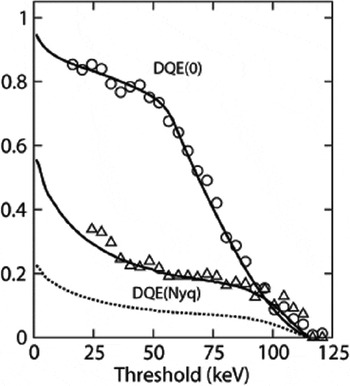
Medipix2 was found to perform very efficiently at 120 keV and at lower energies, with high DQE due to the high signal and virtually noiseless readout. The DQE(0) and DQE at Nyquist frequency as a function of pixel threshold are shown in Fig. 5. The most outstanding feature of this detector is the high value of DQE(0), which is independent of the dose rate, i.e. it is maintained even at extremely low counts. Above 120 keV, the resolution is degraded by the increased lateral spread, relative to the Medipix2 pixel size, of the incident electron trajectories.

Fig. 3.

Experimental (circles) and theoretical (smooth curve) edge spread curves at 120 keV and with four values of threshold settings, equivalent to 12·6, 57·2, 85·5 and 101·8 keV electron energy (McMullan et al. Reference McMullan, Cattermole, Chen, Henderson, Llopart, Summerfield, Tlustos and Faruqi2007). Steeper curves, resulting in a narrower point spread function, indicate improved spatial resolution as discussed further in the text.

Fig. 4.

Experimental and theoretical plots of MTF at Nyquist frequency for 40, 80 and 120 keV energy electrons as a function of threshold (given in units of keV). The experimental values are plotted as data points and simulation results as continuous lines. The horizontal dotted line is drawn at an MTF of 2/π, the maximum possible value of MTF for a pixellated detector (McMullan et al. Reference McMullan, Cattermole, Chen, Henderson, Llopart, Summerfield, Tlustos and Faruqi2007). The inset shows a more conventional plot of MTF as a function of spatial frequency, between zero and Nyquist frequency, for 120 keV electrons with the threshold set to 64·4 keV (highlighted point shown in 120 keV curve in this figure). The dotted line is what one would obtain from a perfect pixellated detector.

Fig. 5.

Experimental values of DQE(0), shown as circles and DQE(Nyquist) shown as triangles, plotted as a function of threshold for 120 keV electrons. The excellent value for DQE(0), independent of count rates, is partly as a result of the noiseless readout (McMullan et al. Reference McMullan, Cattermole, Chen, Henderson, Llopart, Summerfield, Tlustos and Faruqi2007). The maximum possible value of DQE(Nyquist) for a pixellated detector is given by (2/π)²=0·405 and the DQE(Nyquist) values are plotted as a fraction of the maximum possible value. The theoretical value of DQE at Nyquist frequency as a fraction of the maximum possible value is shown as a continuous line and there is good agreement with the experimental curve. The absolute value of DQE(Nyquist) is shown in the dotted line.

4.2.1 Monte Carlo simulation of electron trajectories in Medipix2

The performance of Medipix2, MAPS or indeed any other silicon-based detectors can be predicted with reasonable accuracy, for electrons of different energies using Monte Carlo simulations. Simulations can also help to optimize the detector performance by providing details of the energy loss mechanisms along the electron trajectory. The Monte Carlo simulation method is fairly well known and has been described extensively in several past publications (Joy, Reference Joy1995; McMullan et al. Reference McMullan, Cattermole, Chen, Henderson, Llopart, Summerfield, Tlustos and Faruqi2007, Reference McMullan, Chen, Henderson and Faruqi2009a) and requires only a brief mention.

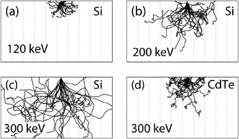
Monte Carlo simulations follow the trajectory and energy loss, of individual electrons of a given energy incident on a detector. The first series of simulations were performed specifically for Medipix2, which has a 300 μm silicon sensor layer, showing electron trajectories at 120, 200 and 300 keV in Fig. 6. The lateral spread of electron trajectories can be compared with the Medipix2 pixel size, which is 55 μm, shown in the figure as faint vertical lines. The energy deposited along the electron track generates electron–hole pairs, which drift in the electrical field applied across the sensor as mentioned above. The scattering curves show that the lateral spread in the electron trajectories increases with the incident electron energy; in fact the spread may be as much as 8–10 pixels in extent at 300 keV, the highest energy for which simulations are shown, resulting in a dramatic reduction in the resolution compared to 120 keV. The lateral spread in electron trajectories can be reduced and spatial resolution improved by using a sensor material such as CdTe, a semiconductor with higher Z number and density (Zwerger et al. Reference Zwerger, Faulera, Fiederle and Jakobs2007; Russo et al. Reference Russo, Lauria, Mettivier, Montesi, Marotta, Aloj and Lastoria2008, Reference Russo, Mettivier, Pani, Pellegrini, Cinti and Bennati2009). It follows that if this technology were to become available in the future, the resolution for 300 keV electrons in CdTe would be expected to be quite similar to that for 120 keV electrons in silicon (see Fig. 6d).

Fig. 6.

(a)–(d) Electron trajectories obtained by Monte Carlo simulations of 120, 200 and 300 keV electrons in 300-μm-thick silicon and 300 keV electrons in 300-μm-thick cadmium telluride sensor. The faint vertical lines are drawn with a 55 μm spacing to highlight the pixel size in a Medipix2 detector. Due to increased range at higher energies there is additional lateral spread of the electrons with consequent loss of resolution (McMullan et al. Reference McMullan, Cattermole, Chen, Henderson, Llopart, Summerfield, Tlustos and Faruqi2007). A high Z and density semiconductor, such as CdTe, would reduce the lateral spread due to decreased range and improved resolution and is shown in (d).

It is possible for an electron entering a pixel near the corner of a pixel to be recorded in several adjacent pixels depending on the spreading of charge. The number of pixels which count an incident electron depends critically on the energy threshold settings for the pixel: for a low threshold, there are likely to be more pixels counting (poor resolution with high efficiency) and for high threshold settings fewer pixels counting (good resolution with lower efficiency). Full discussion on this topic and the procedure for choosing the optimum threshold settings can be found in McMullan et al. (Reference McMullan, Cattermole, Chen, Henderson, Llopart, Summerfield, Tlustos and Faruqi2007).

Monte Carlo simulations are also critical in predicting and understanding the performance of MAPS detectors (McMullan et al. Reference McMullan, Chen, Henderson and Faruqi2009a, Reference McMullan, Faruqi, Henderson, Guerrini, Turchetta, Jacobs and Van Hoftenc). The sensor material is the same as for Medipix2, viz. silicon, although MAPS geometries are very different (Turchetta et al. Reference Turchetta, Berst, Casadei, Claus, Colledani, Dulinski, Hu, Husson, Le Normand, Riester, Deptuch, Goerlach, Higueret and Winter2001). Further details on simulations for MAPS, particularly in improving the expected MTF and DQE by back-thinning, are discussed in Section 4.3.

4.2.2 Applications of Medipix2

As discussed in the previous sections Medipix2 (and similar hybrid detectors) have a number of attractive properties, including a high DQE, even at very low-dose rates, a noiseless readout and high dynamic range which make them attractive for many experiments (Faruqi & Cattermole, Reference Faruqi and Cattermole2005; Typke et al. Reference Typke, Gilpin, Downing and Glaeser2007; Caswell et al. Reference Caswell, Ercius, Tate, Ercan, Gruner and Muller2009; van Gastel et al. Reference Van Gastel, Sikharulidze, Schramm, Abrahams, Poelsema, Tromp and Van Der Molen2009; Glaeser et al. Reference Glaeser, McMullan, Faruqi and Henderson2011). These properties are extremely useful, for example, if an image is to be collected by summing a number of shorter exposure images; since the readout is essentially noiseless the summation adds only the signal without adding extra noise from each image.

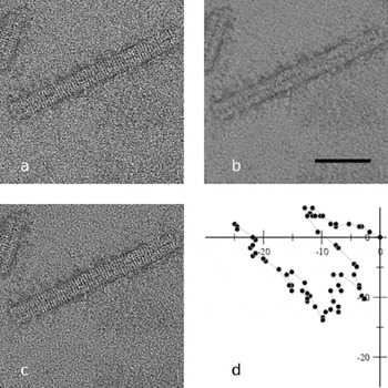
A major reason for lack of high resolution (or image blurring) in cryo-EM is due to beam-induced specimen movement or stage drift during an exposure. Assuming that this effect could be reduced for shorter exposures, a possible solution would be to divide the exposure into a number of shorter period sub-images, which are subsequently added to form the final image. The small movements in the specimen position between the sub-images can be eliminated by aligning the two images prior to summation; this procedure is illustrated in Fig. 7. The test specimen used for illustrating this method was negatively stained (thus quite radiation hard) tobacco mosaic virus (TMV)-coated protein-stacked discs (Klug, Reference Klug1999). A series of 65 one-second images were recorded with Medipix2 in a Philips CM12 microscope at 120 keV. The first image, with an exposure time of 1 s is shown in Fig. 7a and the rather blurred image from the sum of 65 separate 1 s images is shown in Fig. 7b. However, if successive images were aligned prior to summation, using cross-correlation techniques, and the summed image shows much sharper features, Fig. 7c. The amount of movement between images, to produce alignment, as measured by the cross-correlation routine is plotted in Fig. 7d. The specimen drifts for this test were quite large and would not be acceptable for normal microscopy. However, the drift magnitude was ideal for illustrating the power of the technique.

Fig. 7.

(a)–(d) Images of negatively stained tobacco mosaic virus (TMV) coat protein stacked-discs illustrating how short exposure images can be summed provided an appropriate image shift is applied prior to summation: (a) first of 65 one second exposures, (b) sum of all 65 images without alignment, (c) sum of 65 images after alignment, (d) calculated movement of sample, in units of Å (McMullan & Faruqi, Reference McMullan and Faruqi2008). The scale bar shown in (b) is 500 Å in length.

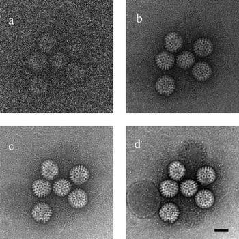
A second example from the same publication (McMullan & Faruqi, Reference McMullan and Faruqi2008) illustrates the very low-dose imaging capabilities of Medipix2. The images of negatively stained rotavirus (Zhang et al. Reference Zhang, Settembre, Xu, Dormitzer, Bellamy, Harrison and Grigorieff2008) recorded at 120 keV under different dose conditions are shown in Fig. 8. The first of a series of 100 images imaged at a dose of 1·6 electron/pixel or 0·04 electron/Ų at the sample is shown in Fig. 8a. Due to the lack of any noise contributions from the detector, it is possible to discern the virus shape even at such low doses. The sum of 100 images, with a total dose of 160 electrons/pixel or 4 electrons/Ų (after alignment) is shown in Fig. 8b; this would be close to a normal dose for a cryo-microscopy experiment. The rotavirus images shown in Fig. 8c and d at 4000 and 64 000 electrons/pixel, respectively, demonstrate the capability of Medipix2 to record images with high dynamic range.

Fig. 8.

(a) Very low-dose (0·04 electron/Ų) images of negatively stained rotavirus. (b) The sum of 100 images shown in (a). (c, d) Images recorded at high doses; for details, see text (McMullan & Faruqi, Reference McMullan and Faruqi2008).

4.3 MAPS based on CMOS technology

MAPS detectors based on CMOS technology were originally developed as a low-power, more economical and technically simpler alternative to CCDs (Fossum, Reference Fossum1993; Janesick et al. Reference Janesick and Putnam2003) for visible light detection. The use of standard CMOS technology means that a given design is not tied to a specific foundry. It also greatly simplifies the implementation of a detector as other components such as analogue to digital converters, control logic and buffer amplifiers can also be incorporated into the detector.

MAPS detectors typically have both higher fixed pattern and readout noise than the scientific grade CCDs; although with recent advances this is no longer necessarily the case. One of the great benefits of using CMOS technology, as opposed to CCD technology, is that it is possible to use special electronics layouts that have far greater radiation hardness than is possible with CCDs. It is, therefore, possible to produce a detector that, while not truly radiation hard, nevertheless has a sufficient lifetime to be used as a practical direct electron detector. Another advantage of MAPS over CCDs is that it is far simpler to implement much faster readouts; an example of the practical usefulness of a faster readout is discussed later in Section 4.3.4 (http://www.cmosis.com/; Janesick et al. Reference Janesick and Putnam2003; McMullan et al. Reference McMullan, Chen, Henderson and Faruqi2009a).

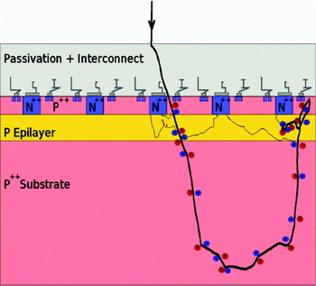
The structure of a typical MAPS detector is shown schematically in Fig. 9. The MAPS chip is manufactured by using a standard heavily p-doped silicon wafer on which there is a lightly p-doped epilayer. This highly ordered layer is typically between 4 and 25 μm thick and forms the sensitive layer of the detector. Radiation incident on the epilayer is detected by the discharge of a capacitor through the collection of mobile electrons associated with the electron–hole pairs generated in the epilayer by the energy lost by the incident radiation. The capacitor consists of a reverse-biased diode formed by an n-type well fabricated into the epilayer. The setting of the voltage on the capacitor and its subsequent readout is controlled by n-MOS transistors fabricated on p-wells deposited on the epilayer adjacent to the n-well diode. The heavy doping of both the p-wells and wafer substrate together generate a potential well in which the movement of electrons in the epilayer is confined. The confinement and long lifetime (resulting from the highly ordered nature of the epilayer) together result in high collection efficiency. However, the lack of any applied bias field means that electrons created near one diode can eventually diffuse to and be collected in a diode further away reducing the spatial resolution. In some more complex MAPS designs, there is an applied field across the epilayer, which results in both a faster signal collection and less charge spreading (Geronimo et al. Reference Geronimo, Deptuch, Dragone, Radeka, Rehak, Castoldi, Fazzi, Gatti, Guazzoni, Rijssenbeek, Dulinski, Besson, Deveaux and Winter2006; Peric, Reference Peric2007).

Fig. 9.

Schematic diagram showing the layout of a single pixel (see text for details). Also shown is the Monte Carlo simulation of a 300 keV electron track, which suffers a backscattering event after traversing the epilayer and generating a signal, which reverses its direction in the substrate and is recorded for a second time (McMullan et al. Reference McMullan, Chen, Henderson and Faruqi2009a) in the epilayer.

As illustrated in Fig. 9, there are three main layers to a MAPS detector: the front or top layer, containing the passivation layer, interconnects, transistors and embedded diodes and p-wells; the thin epilayer acting as the detector; and the bulk substrate that provides strength to the detector but does not play a significant role in signal formation.

To improve our understanding of the operation of MAPS detectors, it was found useful to perform the simulation of the behaviour of individual 300 keV electrons incident on the detector and follow their trajectory; an example of a single trajectory is indicated in Fig. 9. This trajectory is not typical of the majority of 300 keV electrons but represents a significant minority that gets backscattered in the substrate (see also Fig. 6c and Fig. 14). The 300 keV electron enters the epilayer after a small angle deviation in the passivation layer. The energy loss through inelastic collisions of the incident electron creates electron–hole pairs along its track. The excited electrons generated in the epilayer have a long lifetime, and diffuse to the diode to form the output ‘signal’, which can be readout using the pixel electronics.

The application of MAPS to TEM was a logical extension to their role as detectors for minimum ionizing particles (Turchetta et al. Reference Turchetta, Berst, Casadei, Claus, Colledani, Dulinski, Hu, Husson, Le Normand, Riester, Deptuch, Goerlach, Higueret and Winter2001; Faruqi et al. Reference Faruqi, Henderson, Prydderch, Turchetta, Allport and Evans2005a; Milazzo et al. Reference Milazzo, Leblanc, Duttweiler, Jin, Bouwer, Peltier, Ellisman, Bieser, Matis, Wieman, Denes, Kleinfelder and Xuong2005). Similar work on the application of MAPS detectors to EM was also being carried out at other laboratories (Geronimo et al. Reference Geronimo, Deptuch, Dragone, Radeka, Rehak, Castoldi, Fazzi, Gatti, Guazzoni, Rijssenbeek, Dulinski, Besson, Deveaux and Winter2006; Denes et al. Reference Denes, Bussata, Leeb and Radmillovic2007; Deptuch et al. Reference Deptuch, Besson, Rehak, Szelezniak, Wall, Winter and Zhu2007).

4.3.1 Early work on MAPS for EM

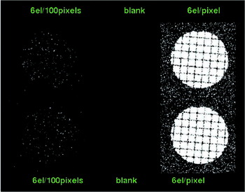
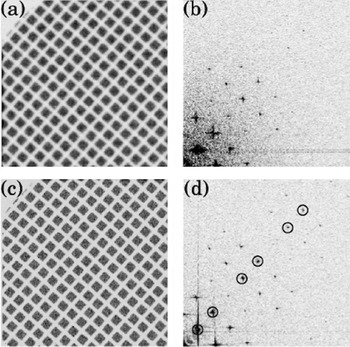
A MAPS detector, designed originally as a startracker for use in optical astronomy by the Rutherford Appleton Laboratory (Prydderch et al. Reference Prydderch, Waltham, Turchetta, French, Holt, Marshall, Burt, Bell, Pool, Eyles and Mapson-Menard2003) was made available by colleagues at that institution for the initial tests and evaluation on a Philips CM12 120 keV electron microscope at the MRC-LMB in Cambridge. The detector contained 525×525 25 μm pixels, had a ~5 μm epilayer, a three-transistor design and used a rolling shutter readout operating at 10 frames/s. As expected from preliminary simulations, the resolution obtained at both 40 and 120 keV as well as the signal-to-noise ratio were very promising. Due to the latter property, it was possible to record single electrons at 40 and 120 keV in this detector as shown in Fig. 10.

Fig. 10.

The left figure shows the image of an EM grid obtained with the Startracker detector at 120 keV, with the electron illumination turned right down to 6 electrons/100 pixels, which ensures that the probability of two adjacent pixels containing a signal is very small. The illumination in the right-hand image is 100 times greater, showing the grid used. Similar experiments done at 40 keV (not shown) displayed slightly improved single-electron images compared to 120 keV images (Faruqi et al. Reference Faruqi, Henderson, Prydderch, Turchetta, Allport and Evans2005a).

A major drawback of the original MAPS detectors, which rapidly became apparent, was that the detectors were not radiation hard and became noticeably damaged by exposure to even relatively small doses (10–20 krad) in the microscope (Faruqi et al. Reference Faruqi, Henderson, Prydderch, Turchetta, Allport and Evans2005a). However, from these early results it was possible to conclude that MAPS detectors represented a very promising future technology for direct electron detection. It was also clear that in order to fulfil this promise, detectors would need to have a greater field of view and be far less sensitive to radiation damage.

Techniques for designing more radiation hard CMOS devices have been known for many years (Campbell et al. Reference Campbell, Anelli, Cantatore, Faccio, Heijne, Jarron, Santiard, Snoeys and Wyllie2001; Eid et al. Reference Eid, Chan, Fossurn, Tsai, Spagnuolo, Deily, Byers and Peden2001; Bogaerts et al. Reference Bogaerts, Dierckx, Meynants and Uwaerts2003; Battaglia et al. Reference Battaglia, Contarato, Denes, Doering, Giubilato, Kim, Mattiazzo, Radmilovic and Zalusky2009a). To test if these were applicable to use in an electron microscope a commercially available radiation-hardened optical MAPS imaging sensor was tested (Faruqi et al. Reference Faruqi, Henderson and Holmes2006). The sensor was much too small for practical use (525×525 pixels) but showed sufficient radiation hardness to clearly demonstrate the possibility of producing larger area MAPS for use in low-dose applications.

4.3.2 Comparison of direct and indirect detectors at 120 and 300 keV

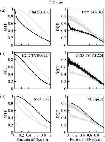
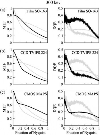
The importance and use of MTF and DQE for describing the properties of detectors were discussed in Section 3; these properties were used in a recent comparison of the most commonly used detectors in EM (McMullan et al. Reference McMullan, Chen, Henderson and Faruqi2009a). In this study, film, CCDs, Medipix2 and MAPS detectors were compared in terms of MTF and DQE as a function of spatial frequency over a range of electron energies (McMullan et al. Reference McMullan, Chen, Henderson and Faruqi2009a). The comparison was restricted to film, CCD (Tietz Video and Image Processing Systems GmbH) and Medipix2 at 120 keV and film, CCD and MAPS at 300 keV. Since different detectors have different pixel sizes, it was considered most convenient to show both MTF and DQE as a function Nyquist (1/2*pixel size) frequency. The MTF results at 120 keV for film are shown in the left-hand column of Fig. 11a, for CCD in Fig. 11b and for Medipix2 in Fig. 11c and the corresponding results for DQE are shown in the right-hand column. Similar results for film, CCD and MAPS at 300 keV are shown in Fig. 12. Full details on these measurements can be found in the original publication (McMullan et al. Reference McMullan, Chen, Henderson and Faruqi2009a). The main conclusion from these comparisons was that, at 300 keV, MAPS showed the maximum potential to be developed into an efficient detector for many applications in EM provided that radiation-hard designs were adopted (Campbell et al. Reference Campbell, Anelli, Cantatore, Faccio, Heijne, Jarron, Santiard, Snoeys and Wyllie2001; Eid et al. Reference Eid, Chan, Fossurn, Tsai, Spagnuolo, Deily, Byers and Peden2001; Bogaerts et al. Reference Bogaerts, Dierckx, Meynants and Uwaerts2003; Battaglia et al. Reference Battaglia, Contarato, Denes, Doering, Giubilato, Kim, Mattiazzo, Radmilovic and Zalusky2009a) and the detector had adequate size (with 4k×4k or more pixels).

Fig. 11.

Six plots showing the MTF in the left column and DQE in the right column as a function of Nyquist frequency for film, CCD and Medipix2 at 120 keV. Each plot is labelled with the name of detector and the plot for this detector is shown in thick black lines whereas the other two as light-grey lines (McMullan et al. Reference McMullan, Chen, Henderson and Faruqi2009a).

Fig. 12.

Six plots showing the MTF in the left column and DQE in the right column as a function of Nyquist frequency for film, CCD and MAPs at 300 keV. Each plot is labelled with the name of detector and the plot for this detector is shown in thick black lines, whereas the other two as light-grey lines (McMullan et al. Reference McMullan, Chen, Henderson and Faruqi2009a).

4.3.3 Improved performance of MAPS for electron detection

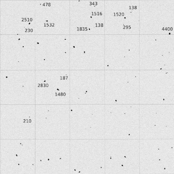
Although MAPS results at 300 keV shown in Fig. 12 are very promising the question arises as to how their performance, in terms of MTF and DQE, could be improved further (see also Denes et al. Reference Denes, Bussata, Leeb and Radmillovic2007; Deptuch et al. Reference Deptuch, Besson, Rehak, Szelezniak, Wall, Winter and Zhu2007). The Monte Carlo simulation of the electron trajectories in silicon, shown in Fig. 6, provides a clue to one possibility that is further illustrated in the simulated trajectory of the electron through a MAPS detector shown in Fig. 9. The incident electron depicted in Fig. 9 is shown to traverse the epilayer, where the signal is generated and recorded; it then proceeds into the ‘inert’ substrate where it is scattered back to the epilayer to generate a second contribution to the signal. The second contribution is in fact larger than the first as the now slower, backscattered electron loses energy at a faster rate per unit distance travelled (Bethe & Ashkin, Reference Bethe, Ashkin and Segré1953). Figure 13 illustrates this behaviour experimentally; it contains a composite figure made up from frames imaged under such low-dose conditions that the probability of a second electron being recorded in the same frame is extremely small. Although some of the events shown consist of a single peak, many are clearly double peaks with a small peak and a larger one that presumably comes from the backscattered contribution. With this detector, the average event results in an analog-to-digital converter (ADC) value of ~260, but there are events with values in excess of 1500 corresponding to the incident electron losing essentially all its remaining energy in the epilayer.

Fig. 13.

A few experimental examples of backscattering events, which show a large signal due to a backscattered electron adjacent to a ‘normal’ signal from the initial traversal. As described in the text, the backscattered electrons create larger signals as they have lower energy. Numbers adjacent to events represent the energy deposited; single traversal events have lower values (~200), but backscattered events values are about an order of magnitude greater (McMullan et al. Reference McMullan, Faruqi, Henderson, Guerrini, Turchetta, Jacobs and Van Hoften2009c).

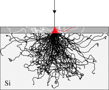
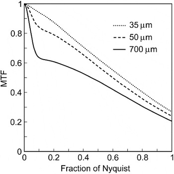
As in previous examples, Monte Carlo simulations were used to improve the understanding of the backscattering process in more detail. In particular, to answer the question: would back-thinning a CMOS detector improve the performance compared to a non-back-thinned detector? Monte Carlo simulations were carried out using 300 keV electrons incident normally on a 350-μm-thick CMOS detector, the first 35 μm shown as dark grey and the remaining part in light grey are shown in Fig. 14 (McMullan et al. Reference McMullan, Faruqi, Henderson, Guerrini, Turchetta, Jacobs and Van Hoften2009c). Electron trajectories in the first 35 μm of silicon are coloured red if they are on their first pass through this layer and white if they have returned to it after being backscattered from the substrate. If the detector were to be thinned to 35 μm only, the red part of the trajectories would contribute and result in not only a lower average signal per electron but also a reduction in the lateral spread in the signal deposited in the detector and consequently an improved MTF. The improvement in MTF with reduced thickness has been measured experimentally by comparing the results for versions of a detector with a thickness of 700, 50 and 35 μm. The experimental results, in terms of MTF as a function of spatial frequency at these thicknesses are shown in Fig. 15, which show very clearly the advantage of using a 35-μm-thick detector. The absence of a sharp drop in MTF at spatial frequencies below 0·1 of the Nyquist frequency for the 35 μm detector indicates that further back-thinning would not produce any significant improvement. The effect on the DQE of the detector is expected to be even more dramatic. Monte Carlo simulations indicate (McMullan et al. Reference McMullan, Chen, Henderson and Faruqi2009a) that on back-thinning to 35 μm the initial drop in DQE with increasing spatial frequency as shown in Fig. 12 would be removed and that the DQE would remain nearly at the zero frequency value out to one-half of the Nyquist frequency. Such a back-thinned detector would benefit from less radiation damage, but more importantly would have a DQE(ω) at 300 keV that, over all spatial frequencies, is better than that of film.

Fig. 14.

Monte Carlo simulation of 300 keV electrons, showing the effect of back-thinning on resolution. The total thickness of the detector is 350 μm and the ‘thinned’ detector, shown in dark grey is 35 μm. Tracks shown in black are in the substrate and do not contribute to the signal. Only tracks shown in red would contribute to the signal in the back-thinned detector; it is interesting to note that there is one backscattering event from the thin epilayer, which appears as a lateral track. The non-back-thinned detector would obtain signal from the red and white tracks, lowering spatial resolution and adding noise at both low and high spatial frequencies (McMullan et al. Reference McMullan, Faruqi, Henderson, Guerrini, Turchetta, Jacobs and Van Hoften2009c).

Fig. 15.

The effect of back-thinning a MAPS detector on the measured MTF as a function of Nyquist frequency. The ‘normal’ detector was 700 μm and the two thinned detectors had a thickness of 50 and 35 μm (McMullan et al. Reference McMullan, Faruqi, Henderson, Guerrini, Turchetta, Jacobs and Van Hoften2009c). Details in text.

4.3.4 Single-event processing

It is possible to improve the performance of CMOS detectors beyond what is achievable with back-thinning by a careful tuning of the epilayer thickness and pixel size in a MAPS detector for a given incident electron energy. The DQE of a traditional integrating detector is fundamentally limited however, by the intrinsic variability of the energy deposited in the thin epilayer by a high-energy-charged particle (Landau, Reference Landau1944; Bichsel, Reference Bichsel1988). Two recent papers have suggested using MAPS detectors in an electron-counting mode similar to that of the Medipix2 detector (Battaglia et al. Reference Battaglia, Contarato, Denes and Giubilato2009b; McMullan et al. Reference McMullan, Clark, Turchetta and Faruqi2009b) discussed earlier. An important difference between the proposed method and Medipix2 is that while the pixels in the Medipx2 count independently, data from a MAPS detector have to be processed frame by frame. The independence of the pixels in Medipx2 allows them to operate in parallel but the trajectory of incident electrons in the sensor coupled with charge sharing between pixels can result in an incident electron being counted in more than one pixel. The resulting variability in the response to an incident electron decreases the DQE. With a MAPS detector it is possible to process events and so avoid this variable counting as discussed in more detail below. To unambiguously identify individual events in a frame requires the number of incident electrons in each frame to be severely restricted. Consequently, many frames are required and to do this in a practical detector will require very high frame rates.

The first of these methods, proposed by Battaglia et al. (Reference Battaglia, Contarato, Denes and Giubilato2009b), deals with the improvement in the point spread function (and hence MTF) that is possible by using event counting (called ‘cluster imaging’ by the authors) over conventional integrating readouts. The method is broadly similar to methods used for recording the centre of gravity of X-ray quanta in multi-wire proportional chambers (MWPC) (Faruqi, Reference Faruqi1988) in X-ray diffraction studies. Provided there is sufficient information on the charge distribution for a given event, the centre of gravity of the distribution provides a much more precise location of the event than a single pixel. Battaglia et al. (Reference Battaglia, Contarato, Denes and Giubilato2009b) used a MAPS detector, which was back-thinned to 50 μm, had 1k×1k 9·5 μm pixels. They used the image of a gold wire to compare the measured line spread function (LSF) at 300 keV obtained using a normal integrating readout and electron counting ‘cluster readout’. The point spread function improved by a factor of 2, a significant factor, when using ‘cluster imaging’ compared to the conventional integrating readout imaging.

McMullan et al. (Reference McMullan, Clark, Turchetta and Faruqi2009b) used a sensor, obtained by courtesy of the RCUK-MI3 collaboration (Allinson et al. Reference Allinson, Anaxagoras, Aveyard, Arvanitis, Bates, Blue, Bohndiek, Cabello, Chen, Chen, Clark, Clayton, Cook, Cossins, Crooks, El-Gomati, Evans, Faruqi, French, Gow, Greenshaw, Greig, Guerrini, Harris, Henderson, Holland, Jeyasundra, Karadaglic, Konstantinidis, Liang, Maini, Mcmullen, Olivo, O'Shea, Osmond, Ott, Prydderch, Qiang, Riley, Royle, Segneri, Speller, Symonds-Tayler, Triger, Turchetta, Venanzi, Wells, Zha and Zin2009; MI3. http://mi3.shef.ac.uk/), with 520×520 25 μm pixels. The sensor includes one ADC for every four columns and full frames could be read out at speeds of up to 148 times per second. The MTF and DQE at 120 keV of this sensor were compared using both integrating and electron counting modes in order to evaluate the ‘enhancement factor’ obtained with the single-electron counting method. An analysis of the observed events, using either their peak position or centroid, leads to substantial improvements in the MTF. The improvement in the MTF at Nyquist frequency was almost a factor of 8 compared to the integration method, as shown in Fig. 16. However, despite this large increase in the MTF, there was no comparable improvement in DQE at the Nyquist frequency. The reason for this shortcoming can be attributed to the fact that electrons do not leave a symmetrical charge distribution as is the case low-energy X-rays. As a result, the observed events cannot be used to accurately determine the incident position of an electron on a detector. In particular, the improvement in the MTF was not sufficient to offset the removal in the decay of the noise power spectra that occurs when an event is localized on to a single pixel.

Fig. 16.

MTF and DQE measured as a function of spatial frequency for three operating modes: integrating mode shown as a solid line, peak position mode shown as dotted (….) line and single-electron mode with renormalization shown as dashed (- - -) lines (McMullan et al. Reference McMullan, Clark, Turchetta and Faruqi2009b).

In order to obtain a higher DQE, McMullan et al. (Reference McMullan, Clark, Turchetta and Faruqi2009b) first identified events and then renormalized their integrated weight to unity. The renormalized events were then treated as a probability distribution for the incident position of an electron. This procedure led to a similar enhancement of the MTF, but the resulting DQE was enhanced over all spatial frequencies; in particular, there was a threefold enhancement of DQE at the Nyquist frequency. To illustrate the improvement in imaging performance obtained with this procedure the authors compared shadow images of an EM grid recorded with the same average number of electrons per pixel using the detector in the conventional integrating and single-electron event modes, shown in Fig. 17. To ensure that the individual events could be distinguished, the individual frames of the single-electron event image were taken at a dose of ~1 electron per 500 pixels. Nearly 8000 frames were required and the image took 55 s to collect.

Fig. 17.

Shadow images of an EM grid obtained in integrating mode (a) and in single-electron mode (c). The FT of the images (only one quadrant shown) are shown in (b) for integrating mode and (d) for single-electron mode. Spots with circles drawn around them in (d) were used for measuring amplitude and signal-to-noise ratio used for DQE values shown in Fig. 18 (McMullan et al. Reference McMullan, Clark, Turchetta and Faruqi2009b).

A comparison of the two methods, shown in Fig. 18 (integrating and single electron events), summarizes the improvement in MTF and DQE obtained. The improvement in MTF is reflected in the greater amplitude of the spots at higher spatial frequencies and the improvement in the DQE by the enhanced ratio in the strength of the spots to that of the surrounding noise.

Fig. 18.

Relative enhancement in MTF and DQE as a function of Nyquist frequency for a single-event processing detector compared to a ‘normal’ integrating detector. The dashed lines in (a) show the enhancements in MTF obtained from Fig. 16. The data points shown as circles are values obtained from the signal-to-noise ratios of spots in the grid shadow images shown in Fig. 17 (McMullan et al. Reference McMullan, Clark, Turchetta and Faruqi2009b).