2.1 Higher block presentation of $\Sigma _A$

For $n\ge 1$ , define a new subshift $\Sigma _A^{(n)}=\Sigma _{A_n}$ , where $A_n$ is a $0\text {-}1$ matrix with rows and columns indexed by $\mathcal {L}_{n}$ given as follows. Set $A_1=A$ and $\Sigma _A^{(1)}=\Sigma _{A}$ . Further, if $n \ge 2$ , then for $X=x_1\cdots x_{n}$ and $Y=y_1\cdots y_{n}\in \mathcal {L}_{n}$ ,

$$ \begin{align*} (A_n)_{XY} :=\begin{cases} 1 & \text{if } x_2\cdots x_{n}= y_1\cdots y_{n-1} \text{ and } X*Y\in \mathcal{L}_{n+1},\\ 0 & \text{otherwise}. \end{cases} \end{align*} $$

There is a conjugacy between the original subshift $\Sigma _A$ and the new subshift $\Sigma _{A}^{(n)}$ via the sliding block code given by $x_1x_2x_3\cdots \ \leftrightarrow \ (x_1\cdots x_{n})(x_2\cdots x_{n+1})(x_3\cdots x_{n+2})\cdots $ .

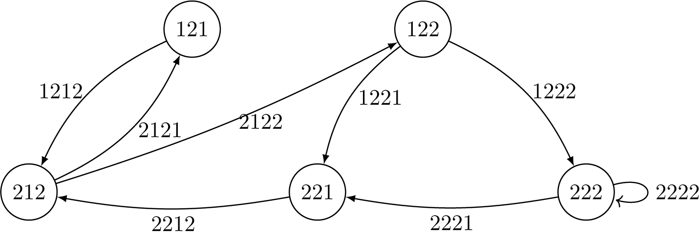
The shift $\Sigma _{A_n}$ is known as the higher block presentation of $\Sigma _A$ of order n. Let ${G_n = (V_n, E_n)}$ denote the graph with adjacency matrix $A_n$ . Here, $V_n = \mathcal {L}_n$ and an edge from the vertex X to Y, whenever it exists, is labeled as $X*Y \in \mathcal {L}_{n+1}$ . The following example illustrates the higher block presentation of an SFT.

Example 2.1. Consider a subshift $\Sigma _A$ with $\Sigma =\{1,2\}$ and $A=\big (\!\begin {smallmatrix}0 & 1\\ 1 & 1\end {smallmatrix}\!\big )$ . Figure 1 shows the graph $G_3$ . The edge from vertex X to vertex Y is labeled by the word $X*Y$ .

Figure 1

The graph $G_{3}$ corresponding to the higher block presentation of $\Sigma _A$ of order 3.

2.2 Markov measure on an SFT

Consider an irreducible SFT $\Sigma _A$ . A row-stochastic matrix is a nonnegative matrix having each row sum to be $1$ . Let $P=(P_{ij})$ be a row-stochastic matrix indexed by $\Sigma $ that is compatible with A, that is, $P_{ij}> 0$ if and only if $A_{ij}=1$ for each $i,j\in \Sigma $ . We now define a measure on $\Sigma _A$ with respect to P, denoted by $\mu _P$ , known as a Markov measure. We know that $1$ is the Perron root of P (which is the largest eigenvalue of P) and the column vector of size N, denoted by $\mathbf {1}$ having all entries $1$ , is the corresponding right Perron eigenvector of P. Let $\textbf {p}=(p_1,\ldots ,p_N)^T$ be a normalized left Perron column eigenvector of P corresponding to Perron root 1, that is, $\textbf {p}^TP=\textbf {p}^T$ and $p_1+\cdots +p_N=1$ . The vector $\textbf {p}$ is known as the stationary vector. Since A is irreducible, the matrix P is also irreducible. Hence, the stationary vector $\textbf {p}$ exists, and is unique and positive by the Perron–Frobenius theorem.

Let $C_w$ be the cylinder based at an allowed word $w=w_1\cdots w_n$ in $\Sigma _A$ . Then, $\mu _P$ is defined on cylinders as $\mu _P(C_w) := p_{w_1}P_{w_1w_2}\cdots P_{w_{n-1}w_n}$ . If $w=w_1$ , then $\mu (C_w) := p_{w_1}$ . By the Kolmogorov extension theorem, this uniquely defines a measure $\mu _P$ on the Borel sigma-algebra generated by cylinders. When the context is clear, we use the notation $\mu $ instead of $\mu _P$ . The measure $\mu $ is a probability measure on $\Sigma _A$ that is invariant under $\sigma $ . We use shorthand $\mu (w)$ to denote the measure $\mu (C_w)$ of $C_w$ . Due to the irreducibility of A, the SFT $\Sigma _A$ is ergodic with respect to $\mu $ .

The Markov measure, which is the unique measure of maximal entropy on $\Sigma _A$ , is known as the Parry measure. It is defined as follows. Let $\textbf {u}=(u_1,\ldots ,u_N)^T$ , $\textbf {v}=(v_1,\ldots ,v_N)^T$ be the positive left and right Perron eigenvectors of the matrix A corresponding to the Perron root $\lambda $ (which is the largest positive eigenvalue of A that exists by the Perron–Frobenius theorem). Define stochastic matrix P as follows. For each $i,j\in \Sigma $ , let $P_{ij}=({A_{ij}v_j}/{\lambda v_i})$ , $p_i=({u_iv_i}/{\textbf {u}^T\textbf {v}})$ . The Parry measure is $\mu =\mu _P$ with P just defined.

2.3 Higher block presentation of the Markov measure $\mu $

We aim to describe the measure on $\Sigma _A^{(n)}$ induced by the Markov measure $\mu _P$ on $\Sigma _A$ that is preserved under the conjugacy between $\Sigma _A$ and $\Sigma _A^{(n)}$ . The induced measure is also a Markov measure. For each $n\ge 1$ , define a matrix $P_n$ indexed by $\mathcal {L}_n$ . For each $X=x_1\cdots x_n$ and $Y=y_1\cdots y_n$ in $\mathcal {L}_n$ , define $(P_n)_{XY}=P_{x_ny_n}$ if $X*Y\in \mathcal {L}_{n+1}$ , and 0 otherwise.

Note that $P_1=P$ . It is easy to check that $P_n$ is a stochastic matrix compatible with $A_n$ and its stationary vector is given by $\boldsymbol {\Lambda }_n=(\mu (X))_{X\in \mathcal {L}_n}$ . That is, $\boldsymbol {\Lambda }_n^T P_n=\boldsymbol {\Lambda }_n^T$ . The measure induced by the Markov measure $\mu _P$ on the higher block presentation $\Sigma _{A}^{(n)}$ of $\Sigma _A$ is nothing but the Markov measure $\mu _{P_n}$ .

Example 2.2. Consider the SFT $\Sigma _A$ with $\Sigma =\{1,2\}$ and $A=\big (\!\begin {smallmatrix}0 & 1\\ 1 & 1\end {smallmatrix}\!\big )$ . Any stochastic matrix $P=(P_{ij})_{1\le i,j\le 2}$ compatible with A satisfies $P_{11}=0$ , and hence, $P_{12}=1$ since P is row stochastic. For $n=2$ , the matrix $P_2$ has size 3, indexed by words from $\mathcal {L}_2=\{12,21,22\}$ . We have

3.1 Adjacency matrix of the open system

Let $\Sigma _A$ be an SFT with a Markov hole $H_{\mathcal {G}}$ . Let r be the length of the longest word in $\mathcal {G}$ . We now define a matrix $B = B_{\mathcal {G}}$ with each of its entries either 0 or 1, as follows. For $r \ge 2$ , the matrix B is indexed by $\mathcal {L}_{r-1}$ , and for each $X,Y\in \mathcal {L}_{r-1}$ , $B_{XY} = 1$ if and only if $X*Y$ belongs to $\mathcal {L}_r$ and does not contain a word from $\mathcal {G}$ . For $r=1$ , we fix the convention that B is a matrix indexed by $\Sigma $ , defined in the same fashion above. The matrix $B_{\mathcal {G}}$ is called the adjacency matrix of the open system. The SFT $\Sigma _{B_{\mathcal {G}}}$ is the collection of all those sequences in $\Sigma _A$ that do not contain words from $\mathcal {G}$ . The matrix $B_{\mathcal {G}}$ is the adjacency matrix of the graph obtained from $G_{A_{r-1}}$ by removing all those edges whose labels contain a word from $\mathcal {G}$ .

Example 3.3. Let $\Sigma =\{1,2\}$ , $A=\big (\!\begin {smallmatrix}0 & 1\\ 1 & 1\end {smallmatrix}\!\big )$ , $\mathcal {G}=\{121,1221\}$ . Since the longest word in $\mathcal {G}$ has length 4, the matrix $B_{\mathcal {G}}$ is indexed by words in $\mathcal {L}_3=\{121,122,212,221,222\}$ . The adjacency matrix corresponding to the hole $H_{\mathcal {G}}$ is given by

3.2 Formula for the escape rate

The following result gives a formula to compute the escape rate into a Markov hole. For any two matrices A and B of the same size, we denote the Hadamard product, or entrywise product of A and B, by $A \circ B$ .

Proof. For simplicity of notation, we use shorthand B for $B_{\mathcal {G}}$ . By the convention discussed in Section 3.1, for $r=1$ , B is indexed by $\Sigma $ , and the rows and columns of B corresponding to the symbols in $\mathcal {G}$ are set to be $0$ . Fix the convention for $r=1$ that $P_{r-1}=P_0=P$ . For $r\ge 2$ , B and $P_{r-1}$ are already defined. Recall from Definition 3.2, $\mathcal {W}_{m}=\{x\in \Sigma _A\ : \ \sigma ^ix\notin H_{\mathcal {G}} \text { for } 0\le i\le m\}$ . For $r\ge 1$ , define the sets,

$$ \begin{align*} S_1 &:= \bigcup\limits_{\substack{X_1, \ldots, X_{m+1} \in \mathcal{L}_{r-1}, \\ X_{i} * X_{i+1} \text{ not containing a word from }\mathcal{G}}}C_{X_1\cdots X_{m+1}} \quad \text{and } \\ S_2 &:= \bigcup\limits_{\substack{X_1, \ldots, X_{m-r+2} \in \mathcal{L}_{r-1}, \\ X_{i} * X_{i+1} \text{ not containing a word from }\mathcal{G}}} C_{X_1\cdots X_{m-r+2}}. \end{align*} $$

It can be easily verified that

(3-1) $$ \begin{align} \mu(S_1) \le \mu(\mathcal{W}_m)\le \mu(S_2). \end{align} $$

Observe that

$$ \begin{align*} \mu(S_1)&=\sum_{\substack{X_1, \ldots, X_{m+1} \in \mathcal{L}_{r-1}, \\ X_{i} * X_{i+1} \text{ not containing a word from }\mathcal{G}}} \mu_{P_{r-1}}(C_{X_1\cdots X_{m+1}}),\\ &= \sum_{X_1, \ldots, X_{m+1} \in \mathcal{L}_{r-1}} \boldsymbol{\Lambda}_{X_1} (B\circ P_{r-1})_{X_1X_2}\cdots (B\circ P_{r-1})_{X_mX_{m+1}}=\sum_{X_1\in \mathcal{L}_{r-1}}\boldsymbol{\Lambda}_{X_1}R_{X_1}^{m}, \end{align*} $$

where $\boldsymbol {\Lambda }$ is the left Perron eigenvector of $P_{r-1}$ and $R^{m}_{X_1}$ denotes the $X_1$  th row sum of $(B \circ P_{r-1})^{m}$ . Similarly,

$$ \begin{align*} \mu(S_2)=\sum_{X_1\in \mathcal{L}_{r-1}}\boldsymbol{\Lambda}_{X_1}R_{X_1}^{m-r+1}. \end{align*} $$

Let $\boldsymbol {\Lambda }_{\min }$ and $\boldsymbol {\Lambda }_{\max }$ denote the smallest and the largest entry of $\boldsymbol {\Lambda }$ . Both are positive since P, and hence $P_{r-1}$ , is irreducible. Thus,

$$ \begin{align*} \boldsymbol{\Lambda}_{\min} \sum (B\circ P_{r-1})^{m} \le \mu(S_1) \le \boldsymbol{\Lambda}_{\max} \sum (B\circ P_{r-1})^{m} \end{align*} $$

and

$$ \begin{align*} \boldsymbol{\Lambda}_{\min} \sum (B\circ P_{r-1})^{m-r+1} \le \mu(S_2) \le \boldsymbol{\Lambda}_{\max} \sum (B\circ P_{r-1})^{m-r+1}, \end{align*} $$

where $\sum (B\circ P_{r-1})^{n}$ denotes the sum of all the entries of the matrix $(B\circ P_{r-1})^{n}$ . By (3-1),

(3-2) $$ \begin{align} \boldsymbol{\Lambda}_{\min} \sum (B\circ P_{r-1})^{m} \le \mu(\mathcal{W}_m)\le \boldsymbol{\Lambda}_{\max} \sum (B\circ P_{r-1})^{m-r+1}. \end{align} $$

Taking logarithm, dividing by m on all terms, and then taking the limit as $m \to \infty $ , we get that the limit $ \lim \limits _{m\rightarrow \infty } ({1}/{m}) \ln \mu (\mathcal {W}_m) $ exists and is given by

$$ \begin{align*} \rho(H_{\mathcal{G}}) = - \lim_{m\rightarrow \infty} \dfrac{1}{m} \ln \sum (B\circ P_{r-1})^m. \end{align*} $$

Since $B \circ P_{r-1}$ is nonnegative, this is further equal to $-\ln \lambda (B\circ P_{r-1})$ . Finally, if A is irreducible, so is $P_{r-1}$ . Since $P_{r-1}$ is a stochastic matrix and $0\le B\circ P_{r-1}<P_{r-1}$ , we have $0\le \lambda (B\circ P_{r-1})<1$ . Hence, $\rho (H_{\mathcal {G}})>0$ .

The above corollary follows from [Reference Haritha and Agarwal22, Theorem 3.1] directly. We give a direct proof when all the words in $\mathcal {G}$ are of length 2.

Proof. Let $\theta $ be an eigenvalue of $B_{\mathcal {G}}$ with eigenvector $w=(w_1,\ldots ,w_N)$ . Then,

$$ \begin{align*}\sum_j(B_{\mathcal{G}}\circ P)_{ij}\frac{w_j}{v_j}=\sum_j(B_{\mathcal{G}})_{ij}P_{ij}\frac{w_j}{v_j}=\sum_j(B_{\mathcal{G}})_{ij}w_j\frac{A_{ij}}{\lambda(A)v_i}=\frac{\theta}{\lambda(A)}\frac{w_i}{v_i}. \end{align*} $$

We have used a simple observation that $(B_{\mathcal {G}})_{ij}A_{ij}=(B_{\mathcal {G}})_{ij}$ . Hence, $\lambda (B_{\mathcal {G}}\circ P)={\lambda (B_{\mathcal {G}})}/{\lambda (A)}$ . The result follows.

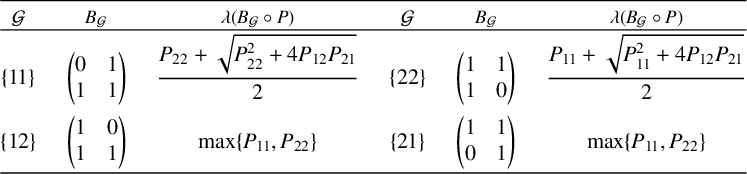
Example 3.6. Consider the full shift on $\Sigma =\{1,2\}$ . That is, $\Sigma =\Sigma _A$ , where A is a matrix of size 2 having all its entries 1. Consider the Markov measure on $\Sigma _A$ given by the stochastic matrix P. First, we consider a single cylinder based at a word of length 2 as the hole. There are four such holes. Table 1 shows the spectral radius calculations.

Table 1

Spectral radius for $B_{\mathcal {G}}\circ P$ for $\mathcal {G}$ consisting of a single word.

Table 1 Long description

The table consists of two identical sets of three columns repeated horizontally.

Column headers from left to right are:

1. G

2. B sub G

3. lambda (B sub G circle P)

4. G

5. B sub G

6. lambda (B sub G circle P)

Row 1 data:

- Column 1: {11}

- Column 2: A 2 by 2 matrix with top row 0, 1 and bottom row 1, 1.

- Column 3: Fraction with numerator P sub 22 plus square root of (P sub 22 squared plus 4 P sub 12 P sub 21) all over 2.

- Column 4: {22}

- Column 5: A 2 by 2 matrix with top row 1, 1 and bottom row 1, 0.

- Column 6: Fraction with numerator P sub 11 plus square root of (P sub 11 squared plus 4 P sub 12 P sub 21) all over 2.

Row 2 data:

- Column 1: {12}

- Column 2: A 2 by 2 matrix with top row 1, 0 and bottom row 1, 1.

- Column 3: max {P sub 11, P sub 22}

- Column 4: {21}

- Column 5: A 2 by 2 matrix with top row 1, 1 and bottom row 0, 1.

- Column 6: max {P sub 11, P sub 22}

Now, consider the hole given by the collection $\mathcal {G}=\{11,122\}$ . Since the length of the longest word of $\mathcal {G}$ is 3, we need to compute the following matrices of size $|\mathcal {L}_2|=4$ : $B_{\mathcal {G}}$ and $P_2$ are indexed by words $11,12,21,22\in \mathcal {L}_2$ . Here,

Hence, $\lambda (B_{\mathcal {G}}\circ P_2)=\max \lbrace P_{22},\sqrt {P_{12}P_{21}}\rbrace $ .

3.3 An upper bound for the escape rate

Our next result (Theorem 3.8) gives an upper bound for the escape rate, in the special case when $\mathcal {G}$ contains a single word. In other words, we look for a lower bound for $\lambda (B_{\mathcal {G}} \circ P_{r-1})$ . We may think of the matrix $B_{\mathcal {G}} \circ P_{r-1}$ as a perturbation of $P_{r-1}$ by changing one of its positive entries to $0$ . To prove this theorem, we recall in the following an important result on the separation of eigenvalues of a nonnegative matrix and its principal submatrices, due to Hall and Porsching.

We know by the Perron–Frobenius theorem that the largest positive eigenvalue of a nonnegative matrix M equals its spectral radius, denoted by $\lambda (M)$ . Let $M(i)$ denote the principal submatrix of M obtained by removing the i th row and the i th column of M.

We now proceed to the following result, which gives an upper bound for the escape rate into a hole, which is a single cylinder.

It is obvious that the escape rate need not be bounded above in general. For instance, when $\mathcal {G}$ consists of all the cylinders of length 2, then $H_{\mathcal {G}}=\Sigma _A$ , in which case, the escape rate is unbounded. We also give an example when $\mathcal {G}$ has two words and the escape rate is not bounded above by $-\ln \theta $ .

4.1 Matrix form of the system of equations (4-1), (4-2)

Let $\Sigma =\{1,\ldots ,N\}$ and $\mathcal {G}$ be a given finite collection of allowed words in $\Sigma _A$ . Denote $\mathcal {G}_1=\{k_1, \ldots , k_m\}$ , $\mathcal {G} \setminus \mathcal {G}_1=\{u_1,\ldots ,u_q\}$ for some $m,\,q \ge 0$ and $\Sigma \setminus \mathcal {G}= \Sigma \setminus \mathcal {G}_1$ as before. We fix the order on each set $\Sigma \setminus \mathcal {G}, \, \mathcal {G}_1$ and $\mathcal {G} \setminus \mathcal {G}_1$ .

Throughout the paper, we denote the identity matrix by $\mathbf {I}$ ; the size is clear from the context. We now write the system of equations (4-1) and (4-2) in matrix form. Recall that $\chi _{a,b}$ equals 1 if $a=b$ and 0 otherwise. The system of equations (4-2) can be written as

(4-3) $$ \begin{align} \mathbf{M}(z) \begin{pmatrix} F(z) \\ G(z) \end{pmatrix} &= \begin{pmatrix} z \mathbf{p}\vert_{\Sigma\setminus \mathcal{G}} \\ \mathbf{0} \end{pmatrix}, \end{align} $$

where $F(z)=(F_i(z))_{i \in \Sigma \setminus \mathcal {G}}^T$ , $G(z)=(G_{u}(z))_{u\in \mathcal {G}\setminus \Sigma }^T$ both are column vectors, $\mathbf {p}\vert _{\Sigma \setminus \mathcal {G}}$ is the vector obtained from the stationary vector $\mathbf {p}$ of P by removing the rows corresponding to symbols in $\mathcal {G}$ , $\mathbf {0}$ is zero vector (column) of appropriate size, and

$$ \begin{align*} \mathbf{M}(z) = \bigg( \begin{array}{c|c} \mathbf{P}(z) & \mathbf{T}(z) \\ \hline \mathbf{E}(z) & \mathbf{C}(z) \end{array}\bigg), \end{align*} $$

with

(4-4) $$ \begin{align} \mathbf{P}(z) = \mathbf{I}-zP^T\vert_{\Sigma\setminus \mathcal{G}}, \ & \ \mathbf{T}(z) = (\chi_{i,t(v)})_{i \in \Sigma\setminus \mathcal{G}, \, v\in\mathcal{G}\setminus \Sigma}, \nonumber\\ \mathbf{E}(z) = (z^{|u|-1}\delta_{u}\chi_{j,i(u)})_{u\in\mathcal{G}\setminus\Sigma, \, j \in \Sigma\setminus \mathcal{G}}, \ & \ \mathbf{C}(z) = -(\tilde{\tau}_{u,v})_{u,v\in \mathcal{G}\setminus\Sigma}, \end{align} $$

where $P\vert _{\Sigma \setminus \mathcal {G}}$ denotes the principal submatrix of P obtained by removing all the rows and columns corresponding to the symbols in $\mathcal {G}$ . Observe that the matrix $\mathbf {T}$ is a $0\text {-}1$ matrix independent of z and records the terminal symbols of words in $\mathcal {G} \setminus \Sigma $ . Moreover, it has a single 1 entry in each column. Further, the matrix $\mathbf {E}(z)$ has a single nonzero entry in each row. The matrix $\mathbf {C}(z)$ records the weighted correlation polynomials of words in $\mathcal {G} \setminus \Sigma $ . Using the matrix form and inverse of a block matrix, we obtain

provided $\mathbf {P}(z)$ and $\mathbf {C}(z)-\mathbf {E}(z)\mathbf {P}(z)^{-1}\mathbf {T}(z)$ are invertible. By Theorems 3.8 and 4.4, $\text {exp}(\rho (H_{\mathcal {G}})$ is a root of $\mathrm {det}(\mathrm {det}(\textbf {P}(z))\textbf {C}(z)-\textbf {E}(z)\mathrm { adj}(\textbf {P}(z))\textbf {T}(z))$ . This is illustrated in Theorem 4.10 for a single cylinder as the hole, in which case, it turns out that $\text {exp}(\rho (H_{\mathcal {G}}))$ is its smallest positive real root. Moreover, in this case, it is exactly the determinant of the matrix $\mathbf {I}-zB_{\mathcal {G}}\circ P_{r-1}$ (see Theorem 4.12).

The following example illustrates the results we have discussed so far.

Example 4.7. Consider the SFT $\Sigma _A$ with Markov measure $\mu _P$ and a Markov hole $H_{\mathcal {G}}$ where

$$ \begin{align*} \Sigma=\{1,2,3\}, \ A=\begin{pmatrix} 1&1&1\\1&1&0\\1&1&1 \end{pmatrix}, \ P=\begin{pmatrix} 1/5&2/5&2/5\\ 9/10&1/10&0\\ 1/10&1/10&4/5 \end{pmatrix}, \ \mathcal{G}=\{12,222,3\} \end{align*} $$

and $\mathbf {p} = (3/11, 2/11,6/11)^T$ is the stationary vector of P.

1. (1) Calculation of escape rate into $H_{\mathcal {G}}$ using Theorem 4.4.

   Let $u=12$ and $v=222$ be the elements of $\mathcal {G}\setminus \Sigma $ . Simple computations give $\tilde {\tau }_{u,v}(z) = \tilde {\tau }_{v,u}(z) =0$ , $\tilde {\tau }_{u,u}(z)=1$ , $\tilde {\tau }_{v,v}(z)=1+z/10$ . Hence, the system of linear equations (4-1), (4-2) can be written as

   $$ \begin{align*} \begin{pmatrix} \begin{array}{c|c} \begin{matrix} 1-\dfrac{z}{5} & -\dfrac{9z}{10}\\[7pt] -\dfrac{2z}{5} & 1-\dfrac{z}{10} \end{matrix} & \begin{matrix} 0 \ \ \ \ & 0\\ 1 \ \ \ \ & 1 \end{matrix} \\[-9pt]\\ \hline\\[-9pt] \begin{matrix} \dfrac{9z}{10} \ \ & 0 \\[7pt] 0 \ \ & \dfrac{2z^2}{100} \end{matrix} & \begin{matrix} -1 & 0 \\ 0 & -1-\dfrac{z}{10} \end{matrix} \end{array} \end{pmatrix} \begin{pmatrix} F_1(z)\\F_2(z)\\G_{u}(z)\\G_{v}(z) \end{pmatrix}=\begin{pmatrix} \dfrac{3z}{11}\\[7pt] \dfrac{2z}{11}\\[7pt] 0\\0 \end{pmatrix}. \end{align*} $$

   Solving these, we get $\mathcal {F}(z) = F_1(z)+F_2(z)=({z(7z^2+80z+250)}/{110(z-5)})$ . The smallest real pole of $\mathcal {F}(z)$ is 5; hence, $\rho (H_{\mathcal {G}}) = \ln (5)$ .

2. (2) Calculation of escape rate into $H_{\mathcal {G}}$ using Theorem 3.4.

   Since $r = 3$ , we need to compute the spectral radius of $B_{\mathcal {G}} \circ P_2$ . Since all the rows and columns having labels containing a word of $\mathcal {G}$ are 0 in $\mathcal {B}_{\mathcal {G}}$ , the spectral radius of $B_{\mathcal {G}} \circ P_2$ is the same as the spectral radius of its submatrix only with rows and columns having labels $11,21$ , and $22$ . The only nonzero entries of this submatrix are $(B_{\mathcal {G}} \circ P_2)_{(11)(11)} = (B_{\mathcal {G}} \circ P_2)_{(21)(11)} = 1/5 \text { and } (B_{\mathcal {G}} \circ P_2)_{(22)(21)} = 9/10$ . Hence, $\rho (H_{\mathcal {G}})=-\ln (\lambda (B_{\mathcal {G}}\circ P_2))=\ln (5)$ . Thus, this method turns out to be much simpler than using the system of equations.

4.2 Escape rate into a cylinder

In this section, we restrict ourselves to the case where the collection $\mathcal {G}$ contains only one word, say $u = u_1 \cdots u_r$ , $r \ge 2$ . Let $\textbf {e}_i$ denote the column vector having its i th entry $1$ and the rest of its entries $0$ . The size of $\textbf {e}_i$ is clear from the context.

Before we proceed to one of our main results for another method to compute the escape rate into a single cylinder, we recall formulas (see [Reference Higham23]) for the inverse and the determinant of the matrix obtained by performing a rank one perturbation to an invertible matrix.

We need the following lemma, which follows from the basic facts of linear algebra.

Theorem 4.10. Let $u=u_1\cdots u_r$ be an allowed word in $\Sigma _A$ of length $r \ge 2$ . Let $z_0$ be the smallest positive real root of the polynomial

(4-5) $$ \begin{align} f_u(z):=\tilde{\tau}_{u}(z)\mathrm{det}(\mathbf{I}-zP)+ z^{r-1}\delta_{u}\mathbf{e}_{u_r}^T\mathrm{adj}(\mathbf{I}-zP)\mathbf{e}_{u_1}, \end{align} $$

where $\tilde {\tau }_{u}(z)=\tau _{u}(z)- z^{r-1} c_{r-1,u,u}\delta _u$ . Then, the escape rate $\rho (C_u)$ into the cylinder based at u with respect to the Markov measure $\mu _P$ is given by $\ln z_0$ .

Proof. Let $\textbf {p}$ be the stationary vector of P. The system of equations (4-3) is given by

$$ \begin{align*} \bigg( \begin{array}{c|c} \mathbf{I}-zP^T& \mathbf{e}_{u_r} \\[-12pt]\\ \hline\\[-10pt] z^{r-1}\delta_u\mathbf{e}_{u_1}^T & -\tilde{\tau}_u(z) \end{array} \bigg)\begin{pmatrix} F(z) \\ G_u(z) \end{pmatrix} = \begin{pmatrix} z\textbf{p}\\ 0 \end{pmatrix}, \end{align*} $$

where $F(z)=(F_1(z)\cdots F_N(z))^T$ . Hence, we can compute that

(4-6) $$ \begin{align} F(z)&= z\tilde{\tau}_u(z)L(z)^{-1}\textbf{p}, \end{align} $$

where $L(z)=\tilde {\tau }_u(z)(\mathbf {I}-zP^T)+z^{r-1}\delta _u\mathbf {e}_{u_r}\mathbf {e}_{u_1}^T$ . Observe that by Lemma 4.8, $\mathrm { det}(L(z))=\tilde {\tau }_u(z)^{N-1}f_u(z)$ , which is a nonzero polynomial in z (for instance, at $z=1$ , it equals $\tilde {\tau }_u(1)^{N-1}f_u(1)=\tilde {\tau }_u(1)^{N-1}\mu (u)\ne 0$ ).

If $\mathbf {I}-zP$ is invertible, using the Sherman–Morrison formula for $L(z)$ (from Lemma 4.8), we get

$$ \begin{align*} L(z)^{-1} =\frac{1}{\tilde{\tau}_u(z)} \bigg((\mathbf{I}-zP^T)^{-1} - \frac{z^{r-1} \delta_u D(z)}{f_u(z)} (\mathbf{I}-zP^T)^{-1} \mathbf{e}_{u_r}\mathbf{e}_{u_1}^T(\mathbf{I}-zP^T)^{-1}\bigg), \end{align*} $$

where $D(z)=\mathrm {det}(\mathbf {I}-zP^T)$ .

Post-multiplying and pre-multiplying $(\mathbf {I}-zP)^{-1}$ in $\textbf {p}^T = \textbf {p}^T P$ and $P\mathbf {1}=\mathbf {1}$ , and substituting $P = ({1}/{z})(zP-\mathbf {I}+\mathbf {I})$ ,

$$ \begin{align*} \sum (\mathbf{I}-zP^T)^{-1}\textbf{p} = \dfrac{1}{1-z}, \sum (\mathbf{I}-zP^T)^{-1} \mathbf{e}_{u_r}\mathbf{e}_{u_1}^T(\mathbf{I}-zP^T)^{-1}\textbf{p}= \dfrac{p_{u_1}}{(1-z)^2}. \end{align*} $$

Substituting these in (4-6),

$$ \begin{align*} \mathcal{F}(z) =\sum_{a\in\Sigma} F_a(z) &= z\tilde{\tau}_u(z) \bigg( \dfrac{1}{1-z} - \dfrac{z^{r-1} \delta_u D(z)}{f_u(z)}\dfrac{ p_{u_1}}{(1-z)^2} \bigg)\\ &= \dfrac{z\tilde{\tau}_u(z)}{(1-z)f_u(z)} \bigg(\!f_u(z)-z^{r-1}p_{u_1}\delta_u\dfrac{D(z)}{1-z} \bigg). \end{align*} $$

Observe that by Lemma 4.9,

$$ \begin{align*} \lim_{z\rightarrow 1} f_u(z)-z^{r-1}p_{u_1}\delta_u\dfrac{D(z)}{1-z} = f_u(1)-p_{u_1}\delta_u \lim_{z\rightarrow 1}\dfrac{D(z)}{1-z} = 0. \end{align*} $$

This implies that $z=1$ is not a pole for $\mathcal {F}(z)$ , which is indeed the case, by Theorem 4.4 since $\text {exp}(\rho (C_u))$ is the smallest pole of $\mathcal {F}(z)$ , which is real and greater than 1. By the form of $\mathcal {F}(z)$ as a rational function, $\text {exp}(\rho (C_u))$ is a real root of $f_u(z)$ . Hence, $\text {exp}(\rho (C_u))\ge z_0$ , which is the smallest real root of $f_u$ . We need to prove that they are equal. Clearly, $z_0>1$ , as otherwise, $\mathcal {F}(z)$ has its smallest pole less than one, which is a contradiction. We consider two cases now.

Case 1. If 1 is the only real positive eigenvalue of P, we have $f_u(z_0)-z_0^{r-1}p_{u_1}\delta _u ({D(z_0)}/{1-z_0})\ne 0$ , and hence, $z_0$ is a pole of $\mathcal {F}(z)$ . Thus, $\text {exp}(\rho (C_u))\le z_0$ .

Case 2. If $\theta $ is the second largest positive real eigenvalue of P other than 1, recalling Theorem 3.8, we know that $\exp (\rho (C_u))\in (1,\theta ^{-1}]$ , and hence, ${z_0\in (1,\theta ^{-1}]}$ . If ${z_0=\theta ^{-1}}$ , then $\text {exp}(\rho (C_u))=\theta ^{-1}$ . However, $f_u(z_0)-z_0^{r-1}p_{u_1}\delta_u\, D(z_0)/(1-z_0)\ne 0$ , if $z_0 \in (1, \theta^{-1})$ , and hence, $z_0$ is a pole of $\mathcal {F}(z)$ . Thus, $\text {exp}(\rho (C_u))\le z_0$ .

The following result states that the escape rate into cylinders based at sufficiently long words can be made arbitrarily small.

The above result can be used to construct a large hole with an arbitrarily small escape rate, as in the following corollary.

4.3 Special cases

In [Reference Bonanno, Cristadoro and Lenci4], Bonanno et al. study the issue of computing the escape rate into a single cylinder in the following two cases: (i) when $\mu _P$ is a product measure; and (ii) when $\Sigma $ has only two symbols and $\mu _P$ is any Markov measure. These cases follow from our results. Let us consider these cases one by one.

1. (i) Let $\mu _P$ be a product measure. Then, $P=\mathbf {1}\textbf {p}^T$ for some probability vector $\textbf {p}$ . Using Lemma 4.8, we get $\mathrm {det}(\mathbf {I}-zP)=1-z$ and $\mathrm {adj}(\mathbf {I}-zP)=(1-z)I+zP$ . Let u be an allowed word of length r. The function $f_u(z)$ defined as in (4-5) takes the form $f_u(z)=\tilde {\tau }_{u}(z)(1-z)+z^{r}\mu (u)$ . In this setting, Theorem 4.4 is precisely the statement of [Reference Bonanno, Cristadoro and Lenci4, Proposition 2.4].

2. (ii) Consider the subshift $\Sigma _A$ with only two symbols with the Markov measure $\mu _P$ , where $P=(P_{ij})_{1\le i,j\le 2}$ . It is easy to see that $f_u(z)=(1-z)(1-(T-1) z)\tilde {\tau }_u(z)+\tilde {\delta }_u z^r +\chi _{u_1u_r}\delta _u(1-Tz)z^{r-1}$ , where $\tilde {\delta }_u=\delta _u P_{u_ru_1}$ and $T=\text {trace}(P)=P_{11}+P_{22}$ . In this setting, Theorem 4.4 is precisely the statement of [Reference Bonanno, Cristadoro and Lenci4, Proposition 4.2].

4.4 Comparison of the two approaches to compute the escape rate

In the preceding two sections, we have presented two different methods to compute the escape rate into a Markov hole $H_{\mathcal {G}}$ in SFT $\Sigma _A$ . The first one, as given in Theorem 3.4, is a direct formula given by $\rho (H_{\mathcal {G}}) = -\ln \lambda (B_{\mathcal {G}}\circ P_{r-1})$ , which depends on the higher block presentation $P_{r-1}$ of the stochastic matrix P (recall r is the length of the longest word in $\mathcal {G}$ ) and the adjacency matrix $B_{\mathcal {G}}$ of the open system. The second method, based on Theorem 4.4, states that the escape rate is the logarithm of the radius of convergence of certain rational functions. Both methods are useful in their own right; one is more applicable than the other depending on the situation. In this section, we highlight some of the advantages of using either of the methods over the other.

In the first formula, the adjacency matrix $B_{\mathcal {G}}$ and the higher-order presentation $P_{r-1}$ of the stochastic matrix P, both are indexed by $\mathcal {L}_{r-1}$ (which is the set of allowed words of length $r-1$ in $\Sigma _A$ ). The sizes of these matrices grow exponentially in r; hence, the method is computationally expensive for large values of r. However, for each fixed r, the formula does not depend on the number of words in the collection $\mathcal {G}$ determining the hole. However, in the second method, the size of the matrix $\mathbf {C}(z)$ (see (4-4)) grows with the number of elements in $\mathcal {G}$ , where $|\mathcal {G}|^2$ many weighted correlation polynomials need to be computed. Hence, for small r and large $|\mathcal {G}|$ , the first method may be more effective. We must point out that the words in $\mathcal {G}$ may have little overlapping and, thus, for large $|\mathcal {G}|$ , the matrix $\mathbf {C}(z)$ may still be easier to compute. Thus, the second method may be computationally less expensive than the first method in certain situations.

In the second approach, to obtain the rational function (the logarithm of its pole is the escape rate), one is required to derive the system of linear equations consisting of as many equations in total as $|\mathcal {G}\setminus \Sigma | + |\Sigma \setminus \mathcal {G}| $ . Hence, the larger the collection $\mathcal {G} \setminus \Sigma $ , the more cumbersome it is to form the required system of equations. However, if the collection $\mathcal {G}$ is small enough, then this approach can prove to be more useful.

In Example 4.7 discussed earlier, computation of escape rate using the first method is much easier than the second. The following example demonstrates a situation where the method of generating functions is better suited.

Example 4.15. Consider the full shift on two symbols with a product measure $\mu _P$ and a Markov hole $H_{\mathcal {G}}$ , with $\mathcal {G}$ consisting of three words each of length r: $u_1=1 1\cdots 12$ , $u_2=2 2\cdots 21$ , $u_3=122\cdots 221$ . We wish to compute the escape rate into the hole $H_{\mathcal {G}}$ . To apply Theorem 3.4, we need to compute the matrix $P_{r-1}$ whose size is $2^{r-1}$ , which grows exponentially with r. However, no matter how large r is, applying Theorem 4.5 is much simpler. We need to solve a system of five linear equations to be able to arrive at a rational function form of $F_1(z)+F_2(z)$ , whose smallest pole is $\text {exp}(\rho (H_{\mathcal {G}}))$ , by Theorem 4.4. Let us now work out the system of equations in the matrix form (4-3), as described in Section 4.1. We have

$$ \begin{align*} M(z)=\begin{pmatrix} 1-zP_{11} & -zP_{21} & 0 & 1 & 1\\ -zP_{12} & 1-zP_{22} & 1 & 0 & 0 \\ z^{r-1}\delta_{u_1} & 0 & -1 & 0 & 1\\ 0 & z^{r-1}\delta_{u_2} & 0 & -1 & 0\\ z^{r-1}\delta_{u_3} & 0 & -z^{r-2}\delta_{u_3}/P_{12} & 0 & -1 \end{pmatrix}. \end{align*} $$

Since $\mu _P$ is a product measure, $P=\mathbf {1}\mathbf {p}$ , where $\mathbf {p}^T=(p_1,p_2)$ is a probability vector. For simplicity of analysis, let $p_1=p_2=1/2$ (uniform measure). Then,

$$ \begin{align*} \mathcal{F}(z) = F_1(z)+F_2(z)=\dfrac{-4^rz^4+2^rz^{3+r}-4z^{1+2r}}{4^rz^3-4^rz^4+8z^{2r}+2^{1+r}z^{2+r}+2^rz^{3+r}-8z^{1+2r}}. \end{align*} $$

Table 2 shows the smallest pole of the above rational function (which is nothing but $\text {exp}(\rho (H_{\mathcal {G}}))$ ), as r varies between 2 and 8, where $\mathcal {G}$ consists of words of length r of the type $u_1 = 1^{r-1}2$ , $u_2 = 2^{r-1}1$ , and $u_3 = 12^{r-2}1$ .

Table 2

Change in escape rate with respect to the length of the words.

Table 2 Long description

The table consists of two rows and eight columns.

Row 1 (Header): The first cell contains the variable r. The subsequent cells list values for r as 2, 3, 4, 5, 6, 7, and 8.

Row 2 (Data): The first cell contains the formula J exp (rho (H sub mathcal G)). The corresponding values for each r are as follows:

* For r = 2, the value is 2.

* For r = 3, the value is 2.

* For r = 4, the value is 2.

* For r = 5, the value is 1.21.

* For r = 6, the value is 1.07.

* For r = 7, the value is 1.03.

* For r = 8, the value is 1.01.

The data shows a plateau at 2 for r values 2 through 4, followed by a non-linear decrease toward 1 as r increases to 8.