
1. Introduction
Unsteady separated and vortex-dominated flows in aerodynamics are particularly important for lifting surfaces during manoeuvring or when they are subject to the unsteady free stream, for example due to turbulence or gusts. These flows are encountered with not only conventional aircraft wings, but also small air vehicles (Mueller & DeLaurier Reference Mueller and Delaurier2003), biologically inspired flows in air and water (Shyy et al. Reference Shyy, Aono, Chimakurthi, Trizila, Kang, Cesnik and Liu2010; Smits Reference Smits2019), and helicopter rotor blades (McCroskey Reference Mccroskey1982). In most of these applications, flow separation rolls up into a leading-edge vortex (LEV), also known as a ‘dynamic stall vortex’, and greatly influences the forces and moments acting on the wing. Leading-edge vortices may increase the time-averaged lift, and therefore may be encouraged on purpose in many engineering applications, such as bio-inspired robotic flows. However, in many other applications, LEVs may cause excessive peak lift, pitching moment and bending moment, which may need to be alleviated. Unsteady aerodynamics in the presence of LEVs is naturally more complex than the thin airfoil theory for non-uniform motion (von Kármán & Sears Reference von Karman and Sears1938).
Generally, studying the unsteady aerodynamics of wings in unsteady motion is easier because of the challenges of producing an unsteady free stream or gusts in experimental studies, since the motion of the wing can be produced with accuracy, while it also serves as a well-defined problem for the computational simulations. Combined motion of pitching and plunging (heaving) wings with a phase angle is the most general case but is more important for optimal propulsive efficiency (Anderson et al. Reference Anderson, Streitlien, Barrett and Triantafyllou1998) as well as aeroelasticity of the wings and airfoils (Theodorsen Reference Theodorsen1935); for example, one may desire to minimise the flow separation at the leading-edge for optimal propulsive efficiency. In contrast, in this paper, we focus on leading-edge vortex formation and dynamics, when the occurrence of an LEV is unavoidable during the unsteady wing motion or in the presence of an unsteady free stream flow. Pure plunging motion is the simplest case, as the unsteady effects act simultaneously along the whole chord-line of the airfoil cross-section, without any motion-induced camber variations. It also represents the limiting case of a streamwise gust with a large wavelength. In addition, the quasi-steady case corresponds to the stationary airfoil set at the geometric angle of attack (unlike pitching motion), making it easier to identify the effects of unsteady motion.
There has been considerable progress in the understanding of LEVs and unsteady forces and moments (McCroskey Reference Mccroskey1982; Ekaterinaris & Platzer Reference Ekaterinaris and Platzer1998; Benton & Visbal Reference Benton and Visbal2019) on two-dimensional (2-D) airfoils. The LEVs can form and shed at small angles of attack for sufficiently high reduced frequencies. However, the significant effects of LEVs are more visible when the airfoil motion extends to the post-stall regime of the static airfoil and the leading-edge flow separation rolls up into concentrated vortical structures. It is not surprising that the largest time-averaged forces and moments occur when the unsteady motion is in, or near, the post-stall flow regime of the static airfoil. Likewise, in the case of plunging airfoils, it is well known that the largest time-averaged lift and fluctuations of the lift are found at a post-stall angle of attack when the LEV formation is easier (Chiereghin, Cleaver & Gursul Reference Chiereghin, Cleaver and Gursul2019). Consequently, we focus on plunging motion at a post-stall angle of attack in this paper.
The existence of a wing tip and tip vortex not only introduces a non-uniformity of the mean flow in the spanwise direction, but also strong three-dimensionality of the LEV as it develops and sheds. Naturally, there may be significant effects on the time-averaged and unsteady forces and moments. Understanding the nature of the three-dimensionality of the LEVs is needed to develop effective flow control methods to limit the excessive forces and moments. The effects of the LEV three-dimensionality may be expected to be more important for low-aspect-ratio wings, as the span of the wing is shorter and the effect of the tip region is felt over a larger portion of the wing. However, a much larger moment arm for the bending moment for high-aspect-ratio wings may produce more significant unsteady effects, while the three-dimensionality of the LEV will be confined to the wing-tip region. A recent review article (Eldredge & Jones Reference Eldredge and Jones2019) has revealed that little is known about the three-dimensionality and instabilities of the LEV filaments on wings.
1.1. Low-aspect-ratio wings
We begin by reviewing the features of LEV three-dimensionality for low-aspect-ratio wings. Previous experiments (Schreck & Helin Reference Schreck and Helin1994; Yilmaz & Rockwell Reference Yilmaz and Rockwell2012) and computational simulations (Spentzos et al. Reference Spentzos, Barakos, Badcock, Richards, Wernert, Schreck and Raffel2005, Reference Spentzos, Barakos, Badcock, Richards, Coton, Galbraith, Berton and Favier2007; Visbal & Garmann Reference Visbal and Garmann2019) revealed the strong three-dimensionality of the LEVs. Various experiments and simulations have been summarized for an aspect ratio of AR = 4 by Chiereghin et al. (Reference Chiereghin, Bull, Cleaver and Gursul2020). The development of a  $\varOmega$-vortex (Schreck & Helin Reference Schreck and Helin1994; Spentzos et al. Reference Spentzos, Barakos, Badcock, Richards, Wernert, Schreck and Raffel2005, Reference Spentzos, Barakos, Badcock, Richards, Coton, Galbraith, Berton and Favier2007) and an arch-type vortex (Visbal & Garmann Reference Visbal and Garmann2019) have also been reported, depending on the value of the reduced frequency. Here, the reduced frequency is k =
 ${\rm \pi}$fc/U∞, where f is the oscillation frequency, c chord length and U∞ free stream velocity. The reduced frequency k can be considered as the ratio of the time scale of the motion to the convective time scale.
Whereas the  $\varOmega$-vortex could be observed for low reduced frequencies (k ≈ 0.05), the arch-type vortex has been reported around k ≈ 0.20 and its leg remains attached and approximately normal to the wing surface. As the reduced frequency is increased to the order of unity (Calderon, Wang & Gursul Reference Calderon, Wang and Gursul2013a; Calderon et al. Reference Calderon, Wang, Gursul and Visbal2013b; Visbal, Yilmaz & Rockwell Reference Visbal, Yilmaz and Rockwell2013), the LEVs are initially approximately two-dimensional as they shed from the leading-edge (unlike for the low reduced frequencies), but exhibit rapid deformation into large arch-type vortices. Depending on the reduced frequency, wing aspect ratio and wing planform shape, one or two arch-type vortical structures may develop from the leading-edge vortices shed on low-aspect-ratio wings.
In the development of the three-dimensionality, tip vortices might play a more significant role than is generally assumed. For even lower aspect ratios, there is a high degree of three-dimensionality in the vortical structures as expected; however, the effect of reduced frequency is equally as important. With increasing reduced frequency, LEVs form quicker and stay longer over the wing as a proportion of the motion period. Although they tend to be more two-dimensional near the leading-edge, they deform much faster due to the induced velocity field of the tip vortices. Reduced frequencies less than 0.2 are generally more relevant to helicopter rotor blades (McCroskey Reference Mccroskey1982); however, reduced frequencies up to k ≈ 1 may be important for gust and turbulence response of large civil transport aircraft (Heathcote, Gursul & Cleaver Reference Heathcote, Gursul and Cleaver2018). The relevant reduced frequency range may further increase for manoeuvring aircraft and for small aircraft encountering small-scale gusts. In the case of travelling gusts or vortices, the spatial velocity gradient of the disturbance determines the equivalent rate of change of effective angle of attack (or plunge rate), which can be large for small-scale gusts and vortices in the atmosphere.
1.2. High-aspect-ratio wings
There is much less published work on the three-dimensionality of LEVs on high-aspect-ratio wings. This may be due to the demanding size of the area/surface of the measured or computed flow domain, although there are some studies focussed on a confined region near the wing tip. For example, surface pressure measurements revealed the three-dimensionality of the leading-edge vortex near the wing tip (Gardner et al. Reference Gardner, Klein, Sachs, Henne, Mai and Richter2014). In another study, surface pressure measurements at selected locations were combined with the unsteady Reynolds-averaged Navier–Stokes (N–S) computations (Kaufmann, Merz & Gardner Reference Kaufmann, Merz and Gardner2017), detailing the differences between the wing-tip region and the inboard sections. It was suggested that multiple dynamic stall cells existed over the span. The effect of the wing-tip region and tip vortex are obvious, even for stationary wings. At a low Reynolds number of Re = 400 and for high-aspect-ratio wings (AR = 8 and 12), Zhang et al. (Reference Zhang, Hayostek, Amitay, He, Theofilis and Taira2020) observed that the natural vortex shedding process at high angles of attack becomes highly three-dimensional, and the 2-D shedding mode co-exists with a new mode near the wing-tip region in the wake.
Flow field measurements for the whole wing are even more sparse in the literature. Recently, volumetric velocity measurements over a high-aspect ratio wing with AR = 10 were presented by Chiereghin et al. (Reference Chiereghin, Bull, Cleaver and Gursul2020). It was shown that the deformation of the LEV filament near the wing-tip region and the movement of the leg inboard caused significant effect on lift force and bending moment. Another important conclusion by Chiereghin et al. (Reference Chiereghin, Bull, Cleaver and Gursul2020) was that the effect on the lift and bending moment grows with increasing reduced frequency. This is likely to be due to increasing circulation of the LEV and tip vortex resulting in larger deformation of the LEV filament. The velocity field measurements by Chiereghin et al. (Reference Chiereghin, Bull, Cleaver and Gursul2020) were carried out for the largest reduced frequency of k = 1.1. In this paper, we extend the range of reduced frequency up to k = 3 and investigate the LEV dynamics.
1.3. Spanwise waves on vortices
Spanwise waves associated with plunging low-aspect-ratio wings have been previously reported (Calderon et al. Reference Calderon, Wang, Gursul and Visbal2013b), with an estimated spanwise wavelength normalized by the chord length of around λz/c ≈ 1. However, this remained unclear as the vortex filament deformation between the wing-tip leg and the wing root was large, and the undulations of the wave were smaller, although the inboard movement of the wave in the spanwise direction was clear. The first evidence of spanwise waves on the leading-edge vortex filament on a high-aspect-ratio wing (AR = 10) has been revealed by the measurements of Chiereghin et al. (Reference Chiereghin, Bull, Cleaver and Gursul2020), although this observation was limited to a swept wing ( $\varLambda$ = 40°). Interestingly, the wavelength of the spanwise wave was also approximately one chord length (λz/c ≈ 1). It is expected that overall deformation as well as the amplitude of the spanwise wave will increase with increasing reduced frequency, and hence the strength of the LEV and tip vortex.
The physical origins of these spanwise waves on LEVs remain unclear. For plunging wings at a post-stall angle of attack, the baseline flow may be considered to be similar to a mixing layer originating from the leading-edge. Therefore, a rough analogy is a forced mixing layer. It is well known that spanwise instabilities develop in unforced mixing layers (Bernal & Roshko Reference Bernal and Roshko1986). The reported wavelength in the spanwise direction, normalized by the wavelength in the streamwise direction, was λz/λx = 0.67 for the naturally developing instabilities. It is not clear if there is any relation between the observations of spanwise waves on plunging wings and streamwise vortical structures in mixing layers (Bernal & Roshko Reference Bernal and Roshko1986) or in wakes (Williamson Reference Williamson1996), or a time-periodic base flow. Recently, Sun, Deng & Shao (Reference Sun, Deng and Shao2018) carried out three-dimensional Floquet stability analysis of the flow over a plunging airfoil set at a zero-mean angle of attack at a Reynolds number of Re = 1700. In their case, the mean flow is jet-like, and hence a propulsive wake rather than a typical wake-like flow at a post-stall mean angle of attack. Both long-wavelength (of the order of λz/c ≈ 1) and short-wavelength (of the order of λz/c ≈ 0.2) spanwise waves were found to be unstable.
Recent numerical simulations investigated the effect of aspect ratio (AR = 4, 8, 16) at Re = 200 000 for a large amplitude pitching motion from 4° to 22° with a reduced frequency of k = 0.20 (Hammer, Garmann & Visbal Reference Hammer, Garmann and Visbal2021). It was found that, with increasing aspect ratio, multiple arch-like cells form and significant effects on unsteady forces and moments are observed. It was suggested that cellular structures were the result of the interaction of the leading-edge vortex with the wing and there was evidence of strong interactions with the trailing-edge vortex as well. The wavelength of these cellular structures was of the order of the chord length. Interestingly, for stationary wings, cellular structures also exist in the oil flow patterns on the upper surface of high-aspect-ratio wings in the post-stall regime (Weihs & Katz Reference Weihs and Katz1983). It is known that the number of cells increases with increasing aspect ratio, with a wavelength of the order of two chord lengths. Weihs & Katz (Reference Weihs and Katz1983) hypothesized that spanwise cells are the result of a Crow-type instability of a vortex pair in the spanwise direction. Furthermore, they assume that the leading-edge vortex sheds naturally in the post-stall regime and forms a pair with its image vortex (as the trailing-edge vortex will be much further away), resulting in one pair of equal strength counter-rotating line vortices. Their application of the Crow instability to this proposed vortex configuration provided an estimated value of a wavelength around two chord lengths. In summary, there are various flow configurations over oscillating and stationary wings that exhibit spanwise periodicity. In particular, for high-aspect-ratio wings or in the airfoil limit (when end-plates or tunnel walls are used in the experiments), the existence of spanwise waves is intriguing, yet not well understood.
1.4. Objectives
Large deformation of the LEV filament and its interaction with the tip vortex for extreme manoeuvres and gust encounters may lead to significant unsteady forces and moments. In this paper, we take a complementary approach to study LEV dynamics on plunging airfoils and high-aspect-ratio wings. The main objectives were to identify the unsteady features of the kinematics of the LEV filament, its spanwise instabilities, and their origin, over a plunging wing with aspect ratio AR = 10, as well as a nominally 2-D airfoil (with end-plates in the experiments), predominantly at a chord Reynolds number Re = 10 000. We first use data from volumetric experimental velocity measurements and direct and implicit large-eddy simulations to identify relevant physics of the dynamic stall process. Subsequently, we consider a reduced model of the LEV in the form of an L-shaped semi-infinite vortex column to highlight the significance of the self-induced motion near the wing-tip region of the dynamic stall process. Finally, we apply stability analysis to investigate vortex flows. Initial findings of our study were presented in Gao, Sherwin & Cantwell (Reference Gao, Sherwin and Cantwell2020) and Son, Wang & Gursul (Reference Son, Wang and Gursul2020, Reference Son, Wang and Gursul2021).
The paper is organized as follows. An overview of the experimental set-up, the measurement method and analysis techniques as well as the numerical approach are given in § 2. Discussion of results is presented in § 3.1 for an overview of the LEV dynamics on the three-dimensional wing, followed by a comparison with the 2-D airfoil cases in § 3.2 for varying kinematic parameters. In § 3.3, we examine the case of the three-dimensional (3-D) wing in detail, paying special attention to the dynamics of the LEV leg near the wing tip and the physical mechanism of the three-dimensionality of the vortex filament. In § 3.4, we clarify the mechanisms present for the 2-D airfoil.
2. Methodology
We investigated plunging airfoils and wings (with aspect ratio AR = 10) set at a fixed post-stall angle of attack of α = 15° in joint experimental and computational simulations. The range of the reduced frequency was k = 0.5 to 3 for the normalised peak-to-peak amplitude A/c = 0.1 and 0.5. The range of the parameters corresponds to the amplitude of the effective angle of attack varying from 2.9° to 56°.
2.1. Experimental methodology
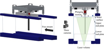
The experiments were performed in the closed-loop free-surface water tunnel facility at the University of Bath. The test section of the water tunnel was 381 × 508 × 1530 mm and the flow velocity range was 0–0.5 m s−1 with a turbulence intensity of less than 0.5 %. The wing was vertically mounted in the test section via the translation stage, which generated a linear motion perpendicular to the free stream flow (see figure 1). An end-plate was used at the root section, therefore the wing represented a half-model for the three-dimensional case. The set-up was identical to the one used in our previous investigations (Chiereghin et al. Reference Chiereghin, Cleaver and Gursul2019, Reference Chiereghin, Bull, Cleaver and Gursul2020). The semi aspect ratio of the wing was sAR = 5, resulting in an effective aspect ratio of AR = 10 for the full wing. A second end-plate was used near the wing tip to eliminate the tip vortex and approximate the 2-D airfoil cases. The chord length of the wing was c = 62.7 mm. The wing was subjected to a sinusoidal plunging motion:
 \begin{equation}H(t) = \frac{A}{2}\textrm{cos(}2{\rm \pi} ft\textrm{),}\end{equation}
where A is the peak-to-peak plunging amplitude. The Reynolds number based on the chord length was Re = 10 000 for the periodic plunging motion. In additional experiments, the transient plunging motion at Re = 20 000 was investigated.
Diagram of the closed-loop free-surface water tunnel facility at the University of Bath, used to obtain the experimental results. The wing is vertically mounted on the translation stage which imposes linear motion perpendicular to the flow. Three-dimensional velocity measurements are obtained from the suction side of the wing using the volumetric velocity measurement system.

The wing had a NACA0012 profile and was manufactured from PA-2200 polyamide using selective laser sintering with a polished smooth surface. A T800 carbon fibre bar with a cross-section of 25 × 5 mm was inserted inside the wing to provide a high spanwise stiffness to the wing. A Zaber LSQ150B-T3 translation stage powered by a stepping motor provided a sinusoidal plunging motion with an accuracy of 2 % of the peak-to-peak amplitude.
Three-dimensional velocity measurements were performed on the volume over the suction side of the wing using the TSI volumetric velocimetry system (V3VTM). One measurement volume covered approximately 40 % of the wing span. Single volume measurements were carried out on a measurement volume centred at the mid-span for the 2-D airfoil case. Multiple volume measurements were used in some of the 3-D wing cases to observe the vortical structures near the tip as well as inboard sections of the wing. The data for multiple volumes were collected separately and then the volumes were merged by using reference points on the wing. The volumes were merged after the interpolation of vectors in each volume. There was an overlap of approximately 4 mm between volumes that corresponded to 1 grid cell. The merging was performed inside this overlapped region by linear interpolation. Volume illumination was achieved with a Nd:YAG 200 mJ pulsed laser. The laser beam was converted to a cone and then the laser cone was projected to the measurement section with a 45 degrees mirror. Water was seeded with 50 μm PSP polyamid seeding particles. The images were acquired using three 4MP 12 bit CCD cameras with Nikkor 50 mm f/1.8D lenses. The cameras were calibrated by translating a rectangular plate of regularly spaced grid dots across the volume of interest with images acquired at 5 mm intervals. The flow images acquired by the cameras were processed in four steps to obtain three components of the velocity fields: particle detection, triplet processing, particle tracking and velocity interpolation to regular grid. The vectors were interpolated using Gaussian weighting. The uncertainty of the measured velocity was estimated to be less than 3 % of the free stream velocity.
Images were acquired at phase intervals of t/T = 0.125, where T is the plunging period, and the flow field was phase-averaged for 50 cycles. The final interpolated volume had a 140 × 140 × 100 mm grid with a uniform voxel size of 4 mm which gave a spatial resolution of 0.063c. The Q-criterion technique was used to identify the three-dimensional vortical structures.
2.2. Computational methodology
Numerical simulations were conducted at Reynolds numbers of 400, 1000 and 10 000. We adopted an implicit large eddy simulation technique which will converge to a direct numerical simulation (DNS) if the flow is sufficiently resolved. In the current simulations, the lower Reynolds number (Re = 400 and 1000) simulations were therefore DNS but the higher Reynolds number (Re = 10 000) simulations should be considered as implicit large eddy simulations where the highest frequencies are damped by the spectral vanishing viscosity technique.
The governing equations are the incompressible Navier–Stokes equations and the continuity equation. To avoid the need for a moving grid, the absolute velocity was solved in the body frame of reference. They are therefore expressed as
 \begin{equation}\left.
\begin{gathered} {\dfrac{{\partial
\boldsymbol{u}}}{{\partial t}} + (\boldsymbol{u} -
{\boldsymbol{u}_B})\boldsymbol{\cdot }\boldsymbol{\nabla
}\boldsymbol{u} ={-} {\rho^{ - 1}}\boldsymbol{\nabla }p +
\nu {\nabla^2}\boldsymbol{u},}\\ {\boldsymbol{\nabla
}\boldsymbol{\cdot }\boldsymbol{u} = 0.} \end{gathered} \right\}\end{equation}
Here, the coordinate system is fixed on the body frame and the body velocity is
 \begin{equation}{\boldsymbol{u}_B} = \frac{{\textrm{d}H(t)}}{{\textrm{d}t}}{\boldsymbol{e}_y}.\end{equation}
On the wing, no-slip boundary conditions are applied and the fluid velocity is imposed as  $\boldsymbol{u} = {\boldsymbol{u}_B}$. At the far field boundaries, the velocity is prescribed as the uniform incoming flow,
 $\boldsymbol{u} = {U_\infty }{\boldsymbol{e}_{x}}$. The wall shear-stress integral is used to calculate the force and the force coefficient is scaled by
 $0.5\rho U_\infty ^2S$, with S being the wing area.
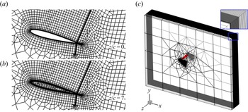
Numerical simulations were conducted using the open-source spectral/hp element framework Nektar++ (Cantwell et al. Reference Cantwell, Moxey, Comerford, Bolis, Rocco, Mengaldo and de Grazia2015). A high-order body-fitted mesh was generated using the open-source software Gmsh (Geuzaine & Remacle Reference Geuzaine and Remacle2009). Figure 2(a) shows the macro elements on the cross-section plane for the A/c = 0.5 case. The 2-D computational domain, which contains 2224 quadrilaterals and 78 triangles, is defined as  $\varOmega = \{ (x,y)|- 20 \le x/c \le 30, - 20 \le y/c \le 20\} $. The height of the first layer of macro elements on the wing surface is 0.003c, and six evenly spaced points are used to represent each curved edge on the wall. Within each element, the polynomial of maximum order of
 $P = 5$ is used for the spectral/hp element expansion.
Macro-element computational meshes for A/c = 0.5 numerical simulations. (a) Two-dimensional macro-element mesh for airfoil, coupled to a Fourier expansion in spanwise direction. (b) Cross-section of 3-D macro-element mesh for wing simulations. (c) Three-dimensional representation of wing mesh, with the wing represented in red. Inset shows high-density of elements in spanwise direction near tip region.

Both infinite wing (airfoil) and finite wing cases were simulated. For the infinite wing, the flow was assumed periodic in the spanwise direction, and a Fourier expansion was adopted along this coordinate axis (known as quasi-3-D). The spectral/hp element mesh in each Fourier plane was the same as the 2-D mesh shown in figure 2(a). For the finite wing case, a 3-D mesh was generated by extruding the 2-D mesh non-uniformly with 72 layers of elements in the region  $0 \le z/c \le 7$ and filling the hollow tip region (see figure 2b) in
 $5 \le z/c \le 7$. Figure 2(c) shows the mesh distribution for the finite-wing A/c = 0.5 cases. The 3-D mesh contains 181 972 hexahedrons and 6598 prisms, which correspond to 40M local degrees of freedom per variable at P = 5. The A/c = 0.1 cases have the same computational domain and mesh structure, but a denser mesh due to its narrower wake.
The first-order velocity correction scheme (Karniadakis, Israeli & Orszag Reference Karniadakis, Israeli and Orszag1991) is used to time-advance the N-S and continuity equations. This expresses the coupled velocity-pressure system as a pressure-Poisson problem and a sequence of velocity-correction Helmholtz problems for each velocity component. For quasi-3-D simulations, the Helmholtz equation is solved using a parallel Cholesky decomposition algorithm of the multi-level statically condensed system (Tufo & Fischer Reference Tufo and Fischer2001). For full 3-D simulations, a left-preconditioned conjugate-gradient iterative method is adopted for the Helmholtz solver to reach an absolute tolerance of 10−5. A low-energy-block preconditioner (Sherwin & Casarin Reference Sherwin and Casarin2001) is used to achieve a parallel efficiency higher than 84 % to up to 3000 cores on ARCHER2, the UK national supercomputer. A successive right-hand side method (Fischer Reference Fischer1998), which extrapolates an optimal initial guess from previous solutions, is also adopted to accelerate convergence. A substepping method, which treats the advection term as a hyperbolic equation using a discontinuous Galerkin formulation, is applied to increase the time step size without violating the CFL constraint of 0.25. The convergence tests are shown in Appendix B.
To improve numerical stability, a spectral vanishing viscosity (SVV) was applied, which also served as the sub-grid scale model of implicit large-eddy simulations. In the spectral/hp element expansion, the SVV has a mimicking DG kernel with coefficient 0.1 (Moura et al. Reference Moura, Aman, Peiro and Sherwin2020). In the Fourier direction, the SVV has an exponential kernel with a cut-off ratio of 0.8.
In postprocessing the numerical results, a Gaussian filter was applied to all instantaneous flow fields to extract large-scale structures. The smoothed velocity field is
 \begin{equation}\tilde{\boldsymbol{u}} = \boldsymbol{u}\ast \frac{1}{{{{\sqrt {2{\rm \pi}} }^3}{\sigma ^3}}}\exp \left\{ { - \frac{{{x^2} + {y^2} + {z^2}}}{{2{\sigma^2}}}} \right\}.\end{equation}
Different filter sizes were tested (see Appendix C, figure 25). The location and circulation of the LEV were not sensitive to  $\sigma $, but the vortex radius and Q isosurface depended on
 $\sigma $. By visual comparison, it was found that
 $\sigma /c = 0.07$ resulted in a similar vortex shape as the phase-averaged field from the experiments.
3. Results and Discussion
3.1. Main features of LEVs on the wing
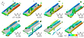
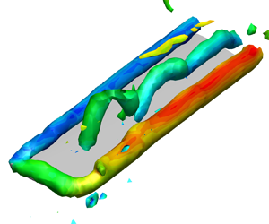
The overview of the vortical structures and the deformation of the LEV obtained from the experiments in a plunging cycle for the wing are presented for k = 2, A/c = 0.5 in figure 3 by plotting the constant Q-surface, coloured by the spanwise vorticity ωz at different phases in the plunging cycle. Here, Q* and  $\omega _z^\ast $ are their dimensionless equivalents, non-dimensionalised using the chord length and free stream velocity. At t/T = 0.250 (when the downward plunge velocity is at its maximum), we observe a newly formed and straight LEV column, a merged tip vortex (TV) and trailing-edge vortex (TEV), and an already deformed LEV from the previous cycle on the wing. The new LEV starts deforming near the wing tip as early as t/T = 0.375 while the leg remains attached to the wing surface. At t/T = 0.625 and later, the leg maintains an angle of approximately 90 degrees to the wing surface. As the leg moves inboard and downstream between t/T = 0.625 and 1.000, the whole vortex filament takes the shape of a spiral, although this helical wave appears to transition to a plane wave at t/T = 1.125. If the same vortical structure is followed at t/T = 0.250 and later, we observe the propagation of the deformation in an inboard direction, while the part near the leg forms an arch-type or upside-down horseshoe vortex, which is similar to the findings for low aspect ratio wings in the literature (see § 1.1). The arch-type vortex remains on the wing until t/T = 0.625 and then sheds downstream. This vortical structure looks similar to that seen on wings with a large radius of gyration (Wolfinger & Rockwell Reference Wolfinger and Rockwell2014; Tudball Smith et al. Reference Tudball Smith, Rockwell, Sheridan and Thompson2017).
Vortical structures (Q* = 5), coloured by spanwise vorticity, around the wing in a plunging cycle for the case of k = 2, A/c = 0.5, obtained from the experiments.

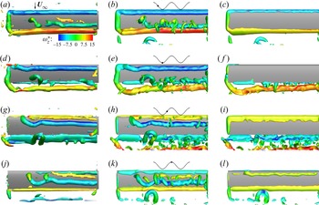
Figure 4 shows the comparison of the experimental and numerical results for the same case of k = 2, A/c = 0.5. The numerical results are filtered using a Gaussian kernel of  $\sigma /c = 0.07$. Both experimental results and numerical results show the isosurface of Q* = 5. In this figure, panels (a,d,g,j) are the experimental results, panels (b,e,h,k) are the top view and panels (c, f,i,l) are the bottom view from the numerical results at the corresponding times t/T = 0.250, 0.500, 0.750, 1.000 (from top to bottom). Excellent agreement between the experiments and simulations is found in the views of the upper surface. It is seen that the leg of the LEV moves slower downstream compared with the straight part further inboard. It is clear in the views of the lower surface from the numerical results that a counter-rotating (counter-clockwise) LEV is also formed over this surface of the wing during the upward motion (at t/T = 0.750 when the upward plunge velocity is maximum). The deformed shape of the LEV on the lower surface at t/T = 1.000 is similar to that of the LEV on the upper surface, but with a short wavelength. The LEV on the bottom surface is trapped around the leading-edge and disappears soon after the wing starts moving downward. The spanwise force distribution of the wing is shown in Appendix E. The variation of the lift distribution is correlated with the deformation of the LEV, while the variation of the drag is small.
Comparison of vortical structures (Q* = 5) from experiments and simulations of a wing for the case of k = 2, A/c = 0.5. Panels (a,d,g,j) are experimental results and panels (b,e,h,k) are numerical results, both showing the top surface at times t/T = 0.250, 0.500, 0.750, 1.000 (from top to bottom). Panels (c, f,i,l) are corresponding numerical results showing the bottom surface, mirrored so that the wing tip is on the left and the leading-edge is on the top for all figures.

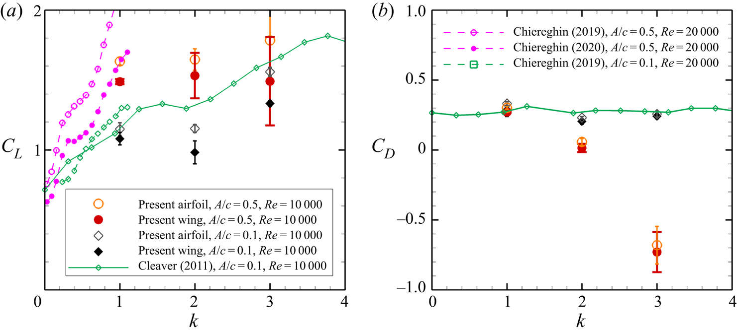
The time-averaged lift and drag coefficients of the plunging airfoil and wing from the simulations are shown in figure 5 as a function of the reduced frequency (we did not experimentally measure the aerodynamic forces in this study). Comparison with the experiments from previous studies (Chiereghin et al. Reference Chiereghin, Cleaver and Gursul2019, Reference Chiereghin, Bull, Cleaver and Gursul2020; Cleaver et al. Reference Cleaver, Wang, Gursul and Visbal2011) for similar parameters is provided. In this figure, the airfoil cases are shown with open symbols and the wing cases are shown with solid symbols. The error bar, which is defined as three times the standard deviation of the mean value in each period, is provided for the numerical results. Good agreement is found between the present numerical results and previous experimental results for the A/c = 0.1 cases. Larger discrepancy for the A/c = 0.5 cases may be an indication of the Reynolds number effect, since this also exists between the experimental results of Chiereghin et al. (Reference Chiereghin, Cleaver and Gursul2019) and Cleaver et al. (Reference Cleaver, Wang, Gursul and Visbal2011). In both experiments and simulations, the airfoil has larger lift than the wing because the latter has a smaller effective angle of attack as well as a truncated (shorter) LEV near the wing tip, which makes it less efficient in generating suction force. However, the drag/thrust forces are similar. This is consistent with the small variation of the spanwise drag distribution in figure 27. For the low-amplitude case, the drag is almost constant as a function of reduced frequency; however, for the larger amplitude, the mean drag becomes mean thrust with increasing reduced frequency.
Lift (a) and drag (b) coefficients as a function of k for the wing (solid symbols) and airfoil (open symbols) in the present study, compared with results from the literature.

In the following section, we study three cases for the wing and airfoil in detail: (k = 1, A/c = 0.5), (k = 2, A/c = 0.5) and (k = 3, A/c = 0.1). These cases have been selected because of the differences in the flow physics of the observed waves on the LEVs. The main parameter appears to be the ratio of the LEV and TEV strengths (circulations) as discussed in detail below. In figure 5, these cases indicate a net mean drag for (k = 1, A/c = 0.5), near neutral (between the net drag and thrust) for (k = 2, A/c = 0.5) and a net mean drag for (k = 3, A/c = 0.1).
3.2. Comparison of the airfoil and wing cases
The measurements revealed that the wing and the airfoil cases differ in the nature, flow physics, the development and the wavelength of the waves on the LEVs. Below we present the three distinct cases captured in the experiments.
Weak LEV and strong TEV (k = 2, A/c = 0.5):
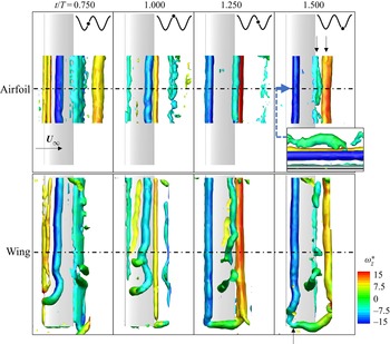
The wing case for these kinematic parameters has already been discussed in figures 3 and 4. In figure 6, we compare the airfoil and the wing cases. For the airfoil case, the data were collected at the mid-span volume (the mid-span plane is shown with a dashed-dotted line) in figure 6. The specific phases t/T are selected so that the development of the LEV for the airfoil case is captured and the LEV exhibits a wave or deformation at the last phase. It is seen that, for the airfoil case, the LEV does not reveal any noticeable deformation while on the airfoil until it reaches the trailing-edge where it rapidly exhibits large deformation and weakening. This instant (t/T = 1.500) is also illustrated in a view from upstream in the small inset, which suggests a bending wave. The two arrows indicate the LEV and TEV at this instant. In contrast, in the wing case, the deformation of the LEV is observed as soon as it forms near the leading-edge (marked by the single arrow at t/T = 1.500 near the wing tip). The deformation mostly occurs near the wing-tip region but can reach the mid-span as the wave propagates inboard (see at t/T = 1.000). No TEV or any other vortex is associated with the formation of the wave.
Comparison of vortical structures (Q* = 5) from experimental data for the airfoil and wing, coloured by spanwise vorticity, for the case k = 2, A/c = 0.5 over one time period. Airfoil data are collected from the mid-span volume only. Inset shows downstream-facing view of the leading edge (Q* = 1). Black arrows on upper-right panel indicate locations of LEV and TEV at instant of strong interaction and weakening. Black arrow on lower-right panel indicates deformation of the LEV shortly after formation.

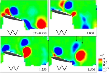
To better observe the vortex interactions for the airfoil case, vorticity contours are plotted at the mid-span plane in figure 7. For the airfoil, the deformation of the LEV is seen inboard near the mid-span. To explain the source of the three-dimensionality, we presented the vorticity slice at the mid-span. The magnitude of the spanwise vorticity is adjusted to make the weak vortices more visible. It can be seen in figure 7 that the LEV (blue) convects downstream between t/T = 0.750 and t/T = 1.000 and reaches near the trailing-edge at t/T = 1.250. The moment of intense and sudden interaction discussed above is also marked in figure 7 by the two arrows. In this case, the TEV is stronger than the LEV, and the timing of the vortices in this interaction (hence, the reduced frequency as a controlling parameter) may be important. We note that the reduced frequency can be considered as the ratio of the time for the free stream to advect one chord length to the time taken for one plunging cycle.
Vorticity from experiments at the mid-span of the airfoil for the case of k = 2, A/c = 0.5 over one time period. Colour scale has been reduced (compared to figure 6) to highlight the presence of weaker vortices. Black arrows on lower-right panel indicate locations of LEV and TEV at instant of strong interaction and weakening.

Similar strength of LEV and TEV (k = 3, A/c = 0.1):
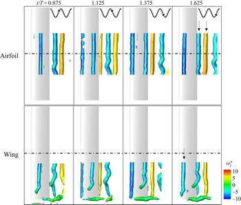
A comparison of the airfoil and the wing cases is presented in figure 8 for the case of k = 3, A/c = 0.1. As we are interested in the deformation near the wing tip for the wing case, we did not see the need to carry out measurements in the inner volume. For the wing case, the deformation of the LEV initially can be seen at t/T = 1.625 (marked by an arrow). As the previous case, the movement of the leg of the LEV and the formation of the helical wave are similar. For the airfoil case, again there is no noticeable deformation of the LEV until it reaches near the trailing-edge. At the instant t/T = 1.625, small deformation in the form of a wave appears on the LEV as it interacts with the TEV (both vortices are marked by arrows). After the LEV sheds into the wake, the amplification of the wave amplitude is seen as it travels downstream.
Comparison of vortical structures (Q* = 5) from experimental data for the airfoil and wing, coloured by spanwise vorticity, for the case of k = 3, A/c = 0.1 over one time period. Airfoil data are collected from the mid-span volume only. Black arrows on upper-right panel indicate locations of LEV and TEV at instant of interaction and deformation of the LEV. Black arrow on lower-right panel indicates deformation of the LEV shortly after formation.

The vorticity contours at the mid-span plane are plotted for the airfoil case in figure 9 to study the interaction of the LEV and TEV. Again, the phase of t/T = 1.625 when the deformation on the LEV is first observed is marked with the arrows to show the interaction of the counter-rotating LEV and TEV pair. For this case, the strength of the interacting LEV and TEV vortices are approximately the same. The deformation of the LEV is not large and sudden compared with the previous case, and the LEV does not disintegrate. Again, this is likely to be controlled by the reduced frequency of the plunging motion. Comparison and discussion of the wavelengths for the airfoil and the wing cases are presented later in the paper.
Vorticity from experiments at the mid-span plane of the airfoil for the case of k = 3, A/c = 0.1 over one time period. Colour scale has been reduced (compared to figure 8) to highlight the presence of weaker vortices. Black arrows on lower-right panel indicate locations of LEV and TEV at instants of interaction and deformation of the LEV.

Strong LEV and weak TEV (k = 1, A/c = 0.5):
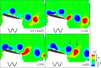
The comparison of the vortical structures on the airfoil and the wing is presented in figure 10. For the wing case, the LEV deformation starts near the wing tip and closer to the leading-edge at t/T = 1.375, which is marked by an arrow. The relative deformation between the leg and the straight part inboard grows at t/T = 1.625 and becomes maximum at t/T = 1.875 (which through periodicity is equivalent to t/T = 0.875). For the airfoil case, the slight deformation of the LEV is first noticed at t/T = 1.625 (marked by arrows), although there is only a weak counter-rotating vortex slightly upstream of the LEV. At the next phase (t/T = 0.875), the LEV is seen in the wake with a larger amplitude of wave.
Comparison of vortical structures (Q* = 4) from experimental data for the airfoil and wing, coloured by spanwise vorticity, for the case of k = 1, A/c = 0.5 over one time period. Airfoil data are collected from the mid-span volume only. Black arrows on upper-right panel indicate locations of LEV and secondary vortex at instants of interaction and slight deformation of the LEV. Black arrow on lower panel indicates deformation of the LEV shortly after formation.

As this case has the lowest reduced frequency of k = 1, we note the slower time scale for the plunging motion to the convection of the LEV over the chord, leading to a different LEV and TEV interaction. The new LEV is formed at t/T = 1.125 and convects downstream at t/T = 1.375. At both phases, multiple vortices may shed from the trailing edge. This is more clearly seen in figure 11, where the spanwise vorticity is plotted with a more suitable scale to amplify the other vortices. At the instant t/T = 1.625, when the deformation of the LEV is first detected (marked by arrows), there is no TEV. Instead, a weak counter-rotating vortex is seen in close proximity to the LEV. The origin of the weak counter-rotating vortex can also be seen earlier at t/T = 1.375, when the secondary vortex starts to develop as a result of the viscous interaction of the LEV with the wing surface. The secondary (and weaker) vortex forms an unequal-strength vortex pair, which results in the deformation as well as the formation of a wave on the LEV as it convects into the wake. For this case, the LEV is stronger than the counter-rotating vortex. Note that, at the next phase t/T = 0.875, the counter-rotating vortex next to the LEV in the wake is a different one, which has just shed from the trailing-edge. Again, the timing and the strength of the LEVs and TEVs are mostly controlled by the reduced frequency.
Vorticity from experiments at the mid-span of the airfoil for the case of k = 1, A/c = 0.5 over one time period. Colour scale has been reduced (compared to figure 10) to highlight the presence of weaker vortices. Black arrows on lower-right panel indicate locations of LEV and secondary vortex at instants of interaction and slight deformation of the LEV.

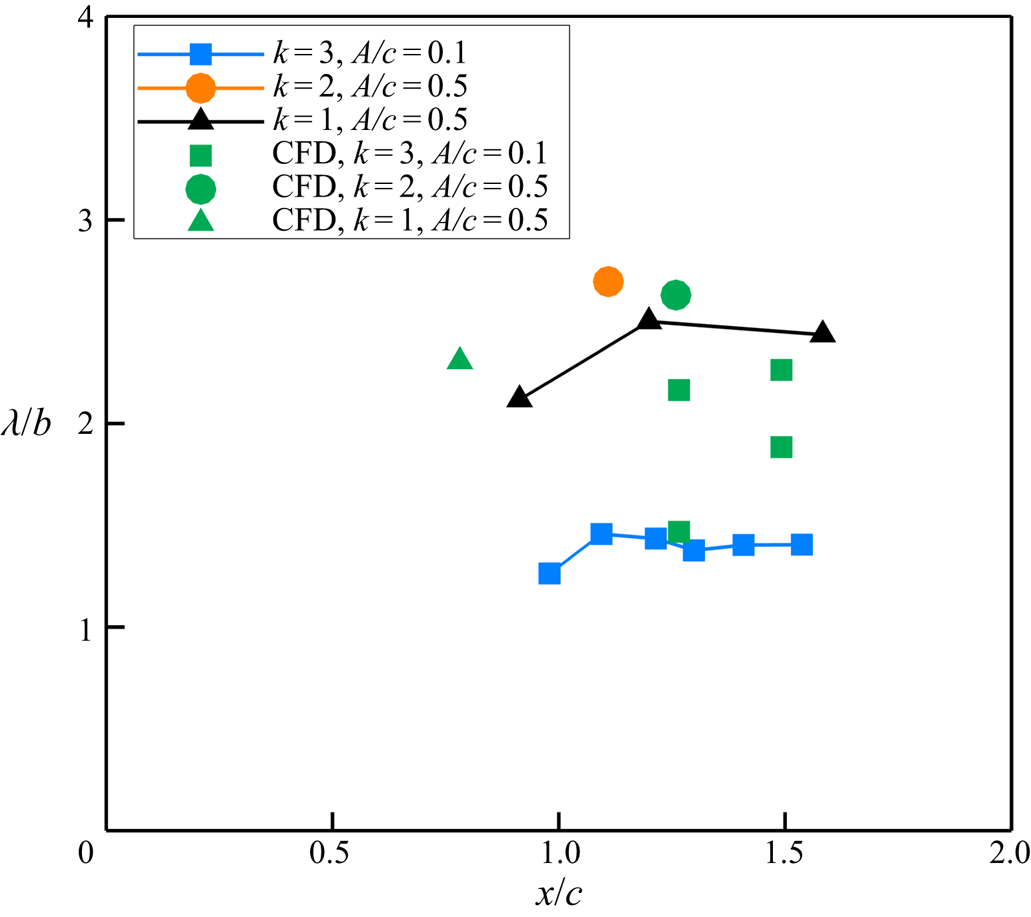
To quantify the LEV dynamics and deformation on the airfoil and the wing, the wavelengths are measured and plotted for the three cases in figure 12. The measurement method, which is based on the identification of the vorticity concentrations in the cross-flow (x = const.) and streamwise (y = const.) planes that pass through the core of the vortex filament, is explained in detail in Appendix A (see figure 23). In figure 12, we plot the measured wavelengths from the experiments and simulations as a function of the streamwise coordinate of the mid-point of the wave. The airfoil cases (open symbols) are found near the trailing-edge (x/c = 1) and further downstream as they are caused by the vortex-pair interactions. The wavelength appears to be roughly constant in the streamwise direction. For some cases, there is only one data point, which indicates that the LEV disintegrated quickly. In contrast, the wing cases (solid symbols) start closer to the leading-edge and may exhibit some increase with the streamwise distance over the wing. In general, the experiments and computational fluid dynamics (CFD) are in a good agreement. The only exception is the case of the airfoil (k = 3, A/c = 0.1) for which there are multiple wavelengths present in the CFD predictions and this is indicated by the scatter of the data points. We note that, as end-plates are used in the experiments, the boundary conditions are not exactly identical for the 2-D simulations. In addition, the phase-averaging in the experiments can mask some scales.
Comparison of wavelengths from experimental data (blue, orange, black) and numerical simulations (green), for the airfoil (open symbols) and wing cases (solid symbols), as a function of the streamwise coordinate of the mid-point of the wave.

Although the dependency of the wavelength on the motion parameters (k and A/c) is apparent, the wavelengths for all cases are of the order of the chord length. It is interesting that, in most cases, the data for the wing converge to those for the airfoil near the trailing edge. The only exception is the case (k = 1, A/c = 0.5) for which the instability wave of the airfoil LEV is caused by the secondary vortex on the wing, rather than the TEV. The different interaction for this case might be the reason for this observation. In the next two sections, the flow physics of the LEV waves on the wing and airfoil will be discussed separately in detail.
3.3. Vortex filament on the wing
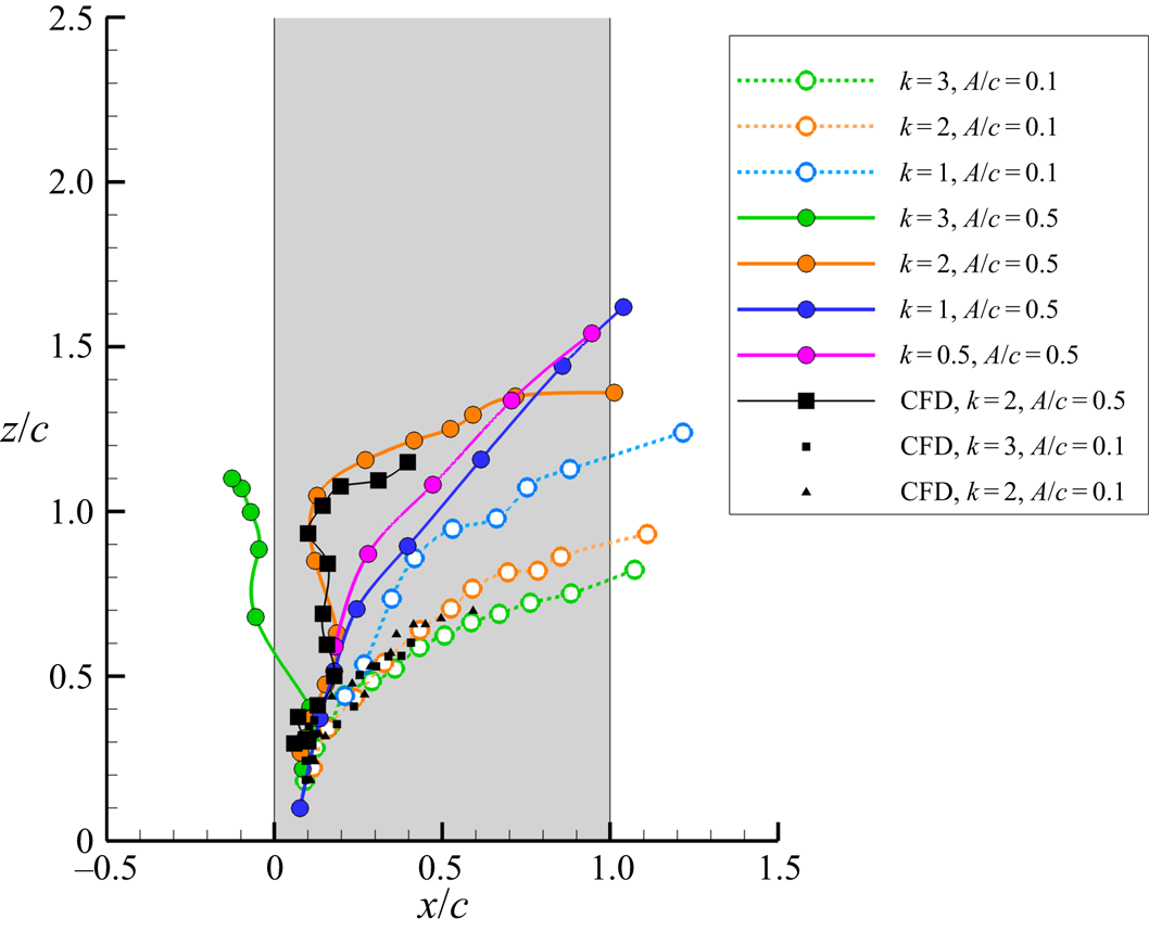
The leg of the LEV starts near the corner of the leading-edge and the wing tip and follows a curved trajectory on the wing surface. The trajectories from the experiments (seven cases) and simulations (three cases) are plotted in figure 13 for various combinations of the reduced frequency k and the normalized amplitude A/c. The simulations and experiments are in a good agreement. As the reduced frequency is increased, the leg tends to move towards the leading-edge for high amplitude (A/c = 0.5) and ultimately, for the case of k = 3, A/c = 0.5, it reconnects with the leading-edge vortex that originates from the lower surface (this case has not been presented in detail in this paper). We also investigated whether the trajectories shown in figure 13 display any correlation with the Strouhal number, defined as St = fA/U∞; however, we could not find any meaningful association. However, the inboard motion of the leg is common in all cases. Although the initial parts of the trajectories collapse, they quickly diverge, with a trend of moving more inboard for the larger A/c value.
Trajectories on the wing surface of the LEV leg for seven combinations of k and A/c through one cycle, obtained through experiments and numerical simulations.

So far, we have presented the periodic plunging wing cases only. In most cases, the vortices shed from the previous cycle may be on, or near, the wing. In addition, it is interesting that these waves are observed in the phase-averaged flow, which means that they are phase-locked to the periodic motion. It is therefore interesting to investigate an impulsively plunged wing.
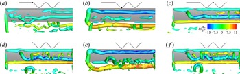
To study the deformation mechanism of the LEV around the tip, a relatively cleaner vortex system was first generated for the stationary flow at the same angle of attack by using numerical simulation. This flow has natural vortex shedding as seen at t = 0 in figure 14. The wing then starts the first period of the sinusoidal motion at k = 2, A/c = 0.5. The vortical flow is shown at t/T = 0.5 and t/T = 1.0 in figure 14. A single LEV is generated together with a connected TEV and TV system. At t = T, the leg of the LEV deforms in a similar way as the periodic motion, but the helical shape is less apparent.
Comparison of vortical structures (Q* = 5), coloured by spanwise vorticity, for transient plunging motion obtained through numerical simulation. Upper panels show transient motion at time points (a) t/T = 0, (b) t/T = 0.5, (c) t/T = 1 and lower panels show periodic motion (d) t/T = 0, (e) t/T = 0.5, ( f) t/T = 1.

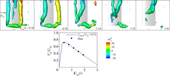
We also carried out controlled transient experiments in the water tunnel. Whereas phase-averaging of the velocity field is applied for the periodic plunging motion, instantaneous velocity field is presented for the transient plunging motion. The wing is stationary at the beginning with an angle of attack of 15°. Then the wing starts its motion and accelerates rapidly, it reaches its peak velocity (Vpmax/U∞ = 0.72) then slows down and stops. The time history of the plunging motion is shown in the inset of figure 15 together with the velocity capture times, marked by small solid circles. The instantaneous vortical structures at the five instants are shown in figure 15. It is seen that there exists similar LEV deformation over the wing in the transient case as in the periodic case. We believe that the instant that the plunging motion commences with respect to the natural vortex shedding will not affect the results. The main reason is that the initial separated flow (vorticity sheet) for the stationary wing does not roll up until further downstream in the absence of any excitation. For the similar cases of transient plunging motions of an airfoil set at post-stall angles of attack (Bull et al. Reference Bull, Chiereghin, Gursul and Cleaver2021), the transient (instantaneous) measurements of the unsteady forces, moments and flow fields were found highly repetitive. The leg is attached to the wing surface and remains behind the vortex column, creating a nearly helical wave while moving downstream. The LEV waves are not limited to the periodic motion, and the transient development of the LEV has a similar mechanism.
Experiments for transient plunging motion with an angle of attack of 15°. Vorticity structures (Q* = 7), starting from an initially stationary wing and coloured by spanwise vorticity, are shown in the top panels. Time history of plunging motion is shown in the lower panel.

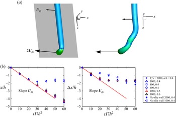
A reduced order model of the deformation of the LEV and the leg in the absence of any plunging or free stream velocity is constructed as below to explain the deformation of the LEV near the tip. A semi-infinite vortex column above a solid plane (both inviscid and viscous walls considered) and attached to the wall at one end (see figure 16(a), left) is used. The existence of the viscous/inviscid solid wall is equivalent to adding a mirror vortex to the semi-infinite vortex column. Due to Helmholtz's vortex theorem that a vortex tube with non-zero circulation cannot terminate inside a fluid, the leg connects the semi-infinite vortex and its mirror vortex, forming an L-shaped vortical filament above the plane. If the TEV and TV are neglected in figure 4, this model is a simplification of the LEV.
Reduced order model for LEV leg dynamics: (a) shape of the L-vortex filament at t = 0 and at a later time; (b) streamwise location of the main vortex filament x and the difference between the main vortex and the leg as Δx as a function of time.

From the Biot–Savart law, the induced velocity of the mirror-vortex on the vortex is
 \begin{equation}{U_{i0}} = \frac{\varGamma }{{4{\rm \pi} h}}.\end{equation}
The velocity induced by the vortex and its mirror vortex at the middle of the vortex leg points to the negative-x or the upstream direction, and has a magnitude of  $2{U_{i0}}$, as indicated in figure 16(a). The self-induced velocity of the main vortex deflects in the negative-x or the upstream direction with a velocity
 ${U_{i0}}$. The development of the vortex filament was numerically simulated for different vortex Reynolds numbers Γ/ν based on the circulation of the vortex, vortex core radius a based on the maximum tangential velocity and the distance above the wall h. The parameters were chosen in a small range around those corresponding to the conditions in figure 4 for the periodically plunging wing. The initial shape of the L-shaped vortex filament at t = 0 is shown in figure 16(a, left). An example of the shape of the vortex filament at a later time is also shown in figure 16(a, right).
Denoting the streamwise displacement of the main vortex filament as a location x, and the difference between the main vortex and the leg as Δx in figure 16(b), we plot x and Δx as a function of time normalised by the height of the vortex above the wall, h, and the vortex circulation Γ. The simulations revealed that, at early times (or for small viscosity and large distance above the wall), the velocities of the main vortex and the leg are consistent with the reduced model. For viscous wall and later times, the appearance of a secondary vortex makes this reduced model no longer valid. The rotational velocity induced by the semi-infinite vortex lifts the deflected vortex leg, and results in the hump shape similar to those in figures 4 and 14. The evolution finally results in the helical vortex leg. In summary, we established that the main mechanism of the motion of the leg and the formation of the helical wave is inviscid in nature, and the image vortex system can explain the observations.
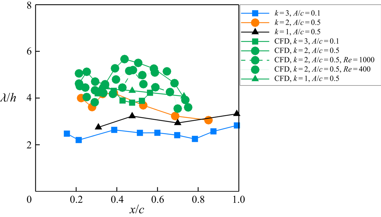
As our reduced order model suggests that the most relevant length scale is the distance of the vortex column above the wall h, we re-plotted the data of the periodically plunging wings presented in figure 12 as λ/h in figure 17. In doing so, we note that h is not constant and generally increases as the LEV travels over the wing. In figure 17, both the experiments and simulations confirm that λ/h remains roughly constant in the streamwise direction and falls in a range of 2 to 6 over the wing. This result again confirms the choice of h as the relevant length scale. We also include simulations at lower Reynolds numbers in this figure, highlighting that the Reynolds number has little effect on the vortex location and the wavelength.
Scaling of wavelength with vortex-to-wall distance h for three combinations of k and A/c through one cycle, obtained through experiments (blue, orange, black) and numerical simulations (green).

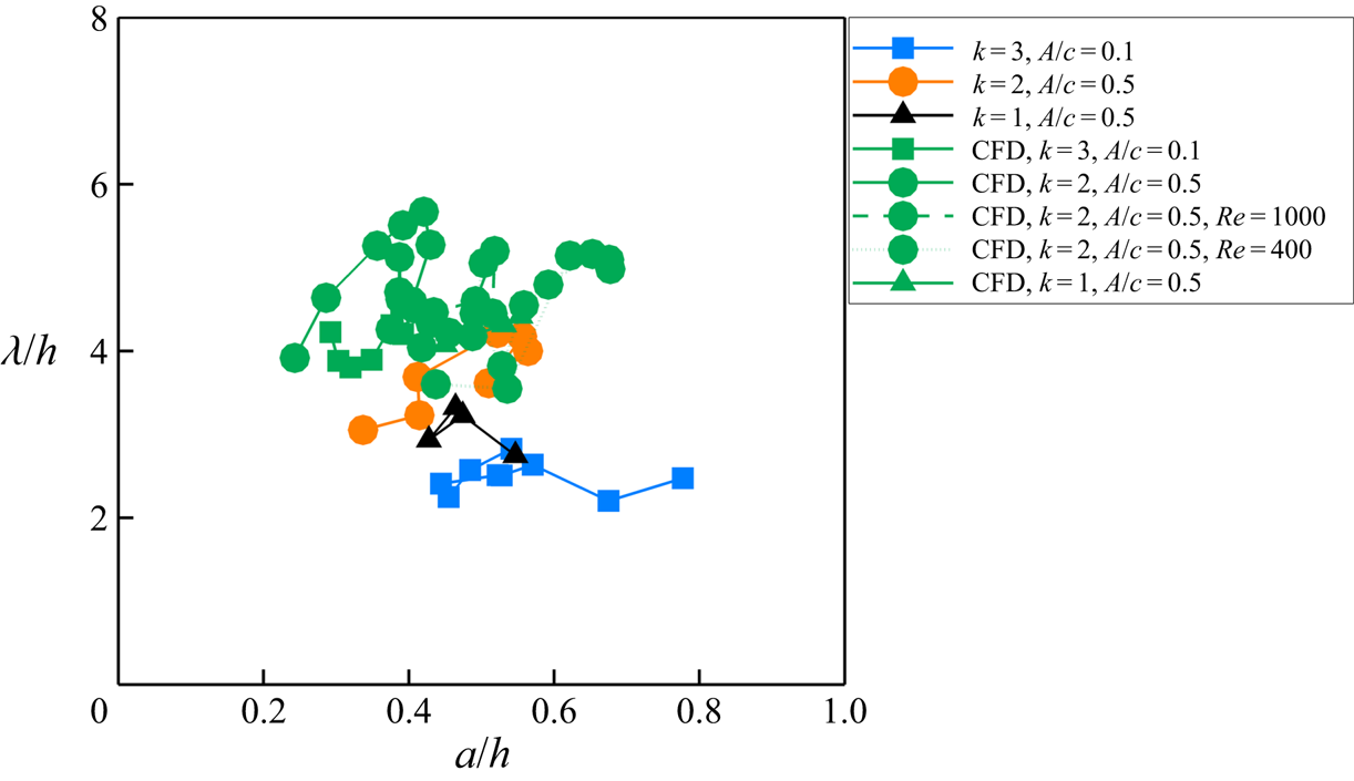
While the normalised wavelength λ/h remains roughly constant, we note that this is a quasi-steady observation as h varies in time and the streamwise location of the wave x/c is equivalent to the time. An alternative variable that does not include time directly is the vortex core radius a normalized by h (noting that a is also time dependent). In figure 18, we present λ/h as a function of a/h for the same data presented in figure 17. Even though there is more effect of the Reynolds number on the core radius in the numerical simulations, the existence of the waves on the wing is linked to a specific range of the normalised core radius a/h.
Scaling of wavelength with core radius a for three combinations of k and A/c through one cycle, obtained through experiments (blue, orange, black) and numerical simulations (green).

3.4. Vortex instabilities on the airfoil
For the airfoil, the LEVs exhibit instabilities near the trailing-edge and downstream, and in all three cases when they come within close proximity of the counter-rotating vortices, either shed from the trailing edge or roll up from the upper surface of the wing as a viscous interaction. Here we focus on the case with the most intense deformation of the LEV. For the case of (k = 2, A/c = 0.5), the numerical simulations and experiments in a smaller measurement volume are compared in figure 19. The wave pattern is clearer near the trailing edge and in the wake in the simulations. When the LEV approaches the trailing edge at t/T = 0.250, it forms a vortex pair with the TEV. The subsequent evolution resembles that of a Crow instability: the weaker vortex has large deformation and evolves into a hair-pin shape with the leg aligning in the streamwise direction (see t/T = 0.750 near the left boundary of the solid-line box). The large deformation of the LEV in the experiments can also be seen in the inset of figure 6.
Vortical structures (Q* = 5), coloured by spanwise vorticity, from experiments (a–d) and numerical simulations (e–h) for the airfoil case of k = 2, A/c = 0.5. Flow from top to bottom.

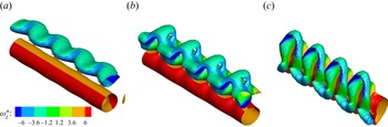
We carried out transient growth stability analysis of a counter-rotating vortex pair with strength ratio 1 : 2 and core radius a = 0.35b, where b is the vortex separation distance, to model this case. In our calculations, we found the transient growth rate approaches the asymptotic result quickly after the evolution time being greater than  $2{\rm \pi}{b^2}{\varGamma ^{ - 1}}$. The asymptotic result is calculated using Crow's theory with the self-induction term of Fabre (Reference Fabre2002). For the total evolution time of
 $6{\rm \pi}{b^2}{\varGamma ^{ - 1}}$, the most unstable wavelength is λ/b = 1.5, compared to λ/b ≈ 0.8 found for an equal strength vortex pair with smaller core size by Leweke & Williamson (Reference Leweke and Williamson1998). Figure 20(a) shows the initial vorticity field at t = 0, where the initial disturbance is the most amplified mode, and figures 20(b) and 20(c) reveal the subsequent evolution at later times. The evolution of the vortex-pair in figure 20 captures the observations in the experiments and numerical simulations.
Stability analysis of a vortex pair, coloured by spanwise vorticity: (a) initial vorticity field at t = 0; (b) and (c) evolution at t = 0.5 and t = 1 (Q* = 1).

The variations of the measured normalized circulation of the LEV and TEV are shown in figure 21(a) for this case. In the experiments, the wave is observed at the instant t/T = 1.5 (see figures 6 and 7). The circulation ratio varies roughly between 1 : 1 and 1 : 3 prior to the appearance of the instability. Naturally, this brings an uncertainty for which instant is chosen for the stability calculations in this quasi-steady approach. To address this issue, we also calculated the growth rate using Crow's theory for other circulation ratios in figure 21(b). The wavelength is scaled by vortex pair separation distance b. For the k = 2, A/c = 0.5 case, the circulation ratio of the LEV–TEV pair varies from 1 to 3 just before t/T = 1.5. However, as seen in figure 21, the corresponding optimal wavelength does not change significantly in this range. As a comparison, the stability diagram of the short-wavelength instability for an (equal-strength) pair of Rankine vortices presented by Leweke & Williamson (Reference Leweke and Williamson1998) in their figure 15 suggests λ/b ≈ 1 for a/b = 0.4 to 0.5, corresponding to our experiments. For the stability calculations in figure 21, the TEV is equal or stronger than the LEV. For the opposite case of strong LEV and weak TEV or when the LEV is paired with the secondary vortex (discussed in § 3.2), the growth rates and the optimal wavelengths will be the same for the vortex-pair instability. Hence, as long as the LEV pairs with a counter-rotating vortex, regardless of the strength ratio, we expect to observe an instability, which is consistent with our observations. As noted by Leweke, Le Dizes & Williamson (Reference Leweke, Le Dizes and Williamson2016), co-rotating vortices are more unstable than counter-rotating vortices for the short-wavelength disturbances. This explains our observations that we only find counter-rotating vortex pairs in all cases studied in detail.
Circulation of LEV and TEV for the experiments of k = 2, A/c = 0.5 (a) and growth rate of vortex pairs with different strength ratios (b) with red line a = 0.4b and black line a = 0.5b.

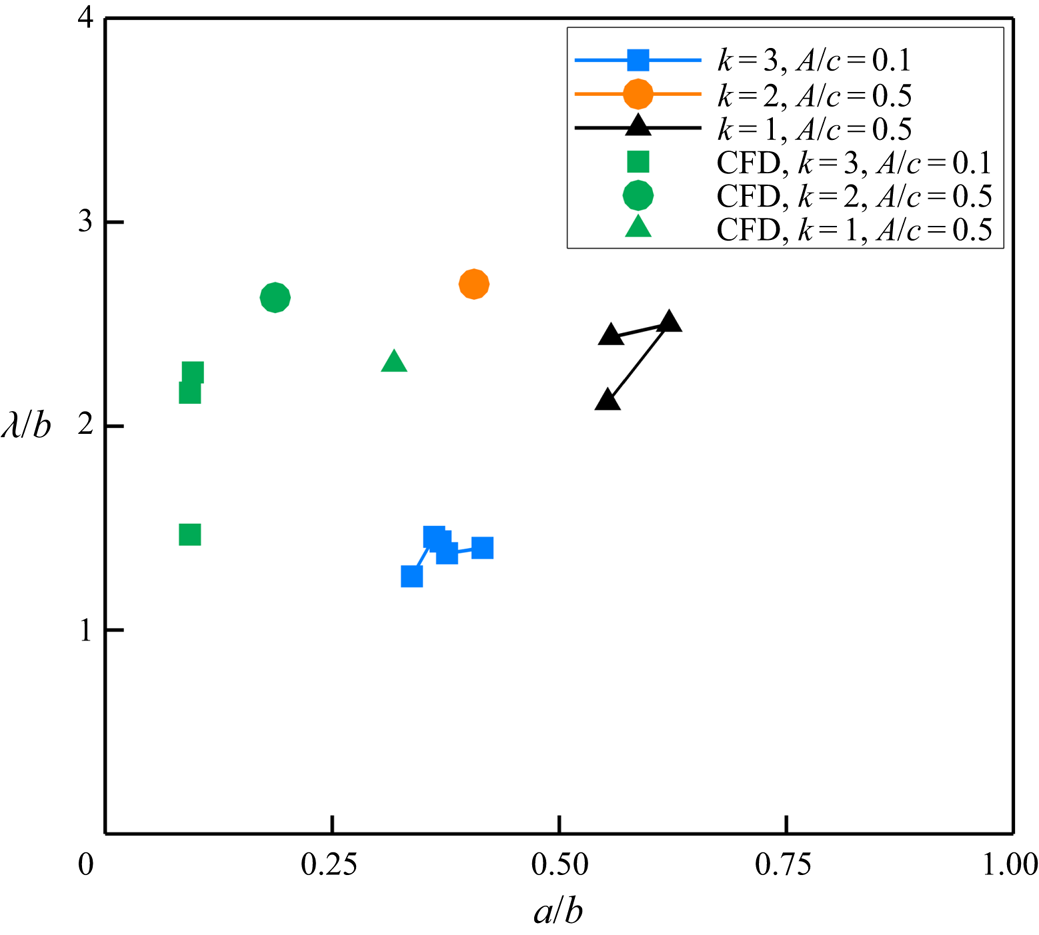
As the most amplified wavelength for counter-rotating vortex pairs of unequal strength is predicted to be weakly dependent on the circulation ratio, we examined how the wavelength scales with the vortex-pair separation distance b. We plot the three cases discussed in § 3.2 as the wavelength normalized by the vortex-pair separation distance b versus the streamwise location of the wave in figure 22. For all three cases, the detected wavelengths are near the trailing edge and downstream. A reasonable agreement is found between experiments and simulations in a narrow range of normalized wavelengths λ/b between 1 and 3. The corresponding variations of λ/b with a/b is discussed in Appendix D (see figure 26).
Wavelength normalized by the vortex separation distance for three combinations of k and A/c from experiments (blue, orange, black) and numerical simulation (green).

4. Conclusions
The vortex dynamics of the LEVs on plunging high-aspect ratio wings and airfoils were investigated by means of volumetric velocity measurements, numerical simulations and stability analysis to understand the deformation of the vortex filament, spanwise instabilities and their origin. The vast majority of the experiments and simulations were at a chord Reynolds number of Re = 10 000 for a wing with aspect ratio of AR = 10 and airfoil oscillating at 0.5 ≤ k ≤ 3.0 and relatively small amplitudes A/c = 0.1 and 0.5. Although both the wing and airfoil cases exhibit spanwise instabilities, these have a fundamentally different origin.
In the presence of a wing tip, the leg of the LEVs remains attached to the wing surface and moves inboard as the spanwise part of the vortex filament travels downstream. The formation of a wave near the leg and close to the leading-edge is apparent. This wave, in most cases, resembles a helical vortex. As the wave travels inboard and downstream, its wavelength may increase. For the parameter range tested (AR, A/c, k), the LEV deformation appears to be limited to roughly 2.5 chord lengths from the tip. Both periodically plunging and transient plunging motions exhibit similar deformation of the vortex filament. A reduced-order model of the filament dynamics was constructed by considering a vortex column over an infinite wall, with the leg attaching to the wall at the initial time. Subsequent deformation of the semi-infinite L-shaped vortex filament under the influence of its mirror image system produced the essential features observed in the experiments and numerical simulations. Hence, the characteristic length was chosen as the distance h of the vortex above the plunging wing, which revealed that the wavelength normalized by h leads to a reasonable collapse of the data, even though both λ and h vary during the cycle.
In contrast, for the airfoil cases, the LEVs exhibit spanwise waves as they get closer to the trailing-edge. In all cases, this coincides with the instant when the LEV gets in close proximity to another counter-rotating vortex, forming a vortex pair. The counter-rotating vortex may originate from the trailing-edge during the plunging motion or may roll-up from the wing surface due to the viscous interaction of the LEV with the wing. The formation time and strength of the counter-rotating vortex, which may be weaker or stronger than the LEV, mostly depends on the reduced frequency of the plunging motion. The stability analysis of counter-rotating vortices of unequal strength has been performed to support our observations.
Acknowledgements
The authors acknowledge the support of Airbus in an advisory role for this project. This work used the ARCHER UK National Supercomputing Service (http://www.archer.ac.uk). This work used the ARCHER2 UK National Supercomputing Service (https://www.archer2.ac.uk).
Funding
The authors acknowledge the Engineering and Physical Sciences Research Council (EPSRC) grant no. EP/S028994/1 and grant no. EP/S029389/1.
Declaration of interests
The authors report no conflict of interest.
Appendix A. Definition of wavelength
To quantify the waves/instabilities and for further detailed investigations on the vortices, the slicing method is applied to the measurement volume (see figure 23). The LEV is cut with x-constant and y-constant planes, and the vorticity component perpendicular to the plane is plotted. When there is deformation of the initially straight vortex filament, this method reveals the curvature of the filament better, and provides more accurate results. For the wavelength measurements, the distance between vortex pairs of the same sign is measured as sketched in the figure. We note that the wavelength that is measured by using the x-constant and y-constant planes to cut through the filament axis gives a projection of the actual wavelength in the spanwise direction. However, the deformation is mostly in the spanwise direction. We estimated the error by comparing with the actual three-dimensional core-to-core distance, which is within 4 %. For the airfoil cases, the wavelength is purely in the spanwise direction. Hence, the method employed in the paper is not only easy to implement in terms of the data analysis, but also gives a suitable comparison with the airfoil cases. The estimated wavelengths from the two different planes are averaged at each phase and presented as a single data point. Their centres (marked with ‘x’ in the figure) are located and other properties, such as core radius, are calculated at these z-constant planes and then averaged. The measurement locations are shown in figure 23 following the motion of the wave. One can see similarities between the LEV leg trajectory in figure 13 and the measurement locations in figure 23. This similarity is expected since the LEV is moving on the wing with its leg attached to the surface, and the wave originates from the leg. The ‘measurement locations’ are the locations of the deforming wave, and the measurements are taken by following the wave.
Method for measuring the wavelength. Planes cutting the LEV (a,b) and the measurement locations (c).

Appendix B. Convergence studies of numerical simulations
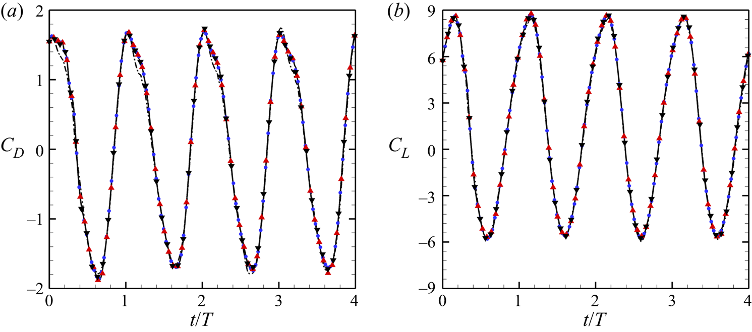
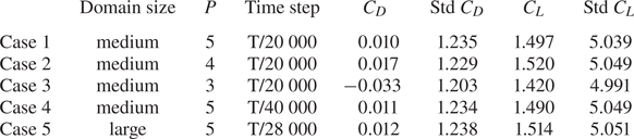
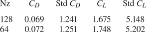
The effects of polynomial order, time step and computational domain are tested for the finite wing at Re = 10 000, k = 2, A/c = 0.5. The results are shown in figure 24 and table 1. The initial conditions for the four cases are the same. Polynomial resolution changes the averaged lift by 2 % (P = 4) or 5 % (P = 3). Time steps change the lift by 0.5 %. Domain size changes lift by 1 %. This indicates the current resolution (case 1) is sufficient.
Convergence study of the drag (a) and lift (b) coefficients for the finite wing as a function of time at Re = 10 000, k = 2, A/c = 0.5. Case 1, black solid line; case 2, black down triangle; case 3, black dash–dotted line; case 4, blue circle; case 5, red up triangle.

Time-averaged force coefficients and their standard deviation of the finite wing at Re = 10 000, k = 2, A/c = 0.5 in four periods. The large domain is  $[ - 30,\; 45] \times [ - 30,\; 30] \times [0,\; 7]$. The medium domain is
 $[ - 20,\; 30] \times [ - 20,\; 20] \times [0,\; 7]$.

The convergence of spanwise resolution for the airfoil is also tested at Re = 10 000, k = 2, A/c = 0.5. Results are shown in table 2. The current spanwise resolution with 128 planes is sufficient.
Time-averaged force coefficients and their standard deviation of the airfoil at Re = 10 000, k = 2, A/c = 0.5 in four periods.

Appendix C. Smoothing of numerical results in post-processing
The effect of  $\sigma $ of the Gaussian filter is shown in figure 25. For the unfiltered numerical results, the main LEV has a very thin vortex core, but it is difficult to identify due to the many small-scale vortices. Filtering with an increasing
 $\sigma $ results in a thicker vortex core, but the main vortex is also clearer. It is found that the radius of the LEV increases with
 $\sigma $, as it should be in theory. The total circulation and vortex location are almost invariant with
 $\sigma $.
Effect of filter size on vortical structures (Q* = 5), coloured by spanwise vorticity: (a)  $\sigma /c = 0.10$; (b)
 $\sigma /c = 0.07$; (c)
 $\sigma /c = 0.05$; (d) no filter.

Appendix D. Core radius versus core-to-core distance
Parametric variation of the wavelength as a function of ratio of the core radius to the vortex separation distance is given in figure 26. A reasonable agreement between the CFD and the experiments is found in the range of λ/b, but there is a wider spread in a/b, which shows the insensitivity to the core radius.
Parametric variation of wavelength for vortex pairs for three combinations of k and A/c obtained from experiments (blue, orange, black) and numerical simulation (green).

Appendix E. Spanwise force distribution of the wing
The spanwise force distribution of the finite wing is shown in figures 27(a,d,g,j). The instantaneous flow fields from figure 4 are also given in this figure in a way that the wing tip corresponds to z/c = 5 and the wing root to z = 0. For the finite wing, the section force coefficient reduces to a small value at the wing tip but, due to the finite thickness of the wing, this value is not exactly zero. The variation of the sectional lift coefficient is correlated with the deformation of the LEV and the vortex leg of the LEV generates a local maximum lift. The variation of the drag is small. The variation of the sectional drag coefficient is small.
Results for Re = 10 000, k = 2, A/c = 0.5. Panels (a,d,g,j) are the sectional lift and drag coefficients, panels (b,e,h,k) are the top view and panels (c, f,i,l) are the bottom view from the numerical results at t/T = 0.250, 0.500, 0.750, 1.000 (from left to right). The bottom view is mirrored so that the wing tip is on the left and the leading-edge is on the top for all figures (Q* = 5).