1 Introduction
Bubbly flows play an essential role in a large number of technical applications, such as in boiling water reactors (nuclear industry), in air lift pumps (oil industry) and particularly so with chemical reactors (process industry). Computational fluid dynamics (CFD) has become an indispensable engineering tool for the analysis and design of such systems, due to the consistent rise of computational power over the last decades. Direct numerical simulation (DNS), resolving all length and time scales of fluid turbulence without significant modelling assumptions, is now feasible for moderate Reynolds number or for reduced-complexity two-phase flows. The case investigated here is of the latter category – technically relevant bubble Reynolds number, but of a limited complexity as it exhibits only two bubbles. While this study is primarily aimed at improving the fundamental understanding of turbulent two-phase flows, the insights are likely to be useful for usual CFD modelling methodologies, e.g. large-eddy simulation (LES). A particular focus is placed on liquid–gas interface dynamics and associated turbulence production (in the wake of the bubbles). An accurate reproduction of such effects is of pivotal importance with regard to the bubble–bubble interactions in swarm-like flows.
Having indicated that two-phase turbulence behaves differently from single-phase turbulence in some aspects, several existing analyses are reviewed here. Particularly in the case of the bubble-induced turbulence (BIT), at least three potential fluctuation sources have to be taken into account: the unsteadiness of bubble deformation, the bubble trajectory, and vortex shedding in the bubble wake. In the seminal work of Lance & Bataille (Reference Lance and Bataille1991) on bubbly air–water flows, it was found that the spatial spectrum of the turbulent kinetic energy in the inertial subrange followed a
 $-8/3$
power law rather than the classical
 $-5/3$
power law known from single-phase turbulence. Using a scaling argument, Lance & Bataille (Reference Lance and Bataille1991) also arrived at a power-law exponent of
 $-3$
, which is close to the experimentally determined value of
 $-8/3$
. The structure and dynamics of bubble wakes were investigated in detail by Brücker (Reference Brücker1999). His experiments focused on ellipsoidal bubbles in the diameter range of 4–8 mm, featuring spiral, zigzag and rock trajectories during their motion in water under counterflow conditions. It was shown that the zigzagging motion was associated with a regular generation and discharge of alternate, oppositely oriented, hairpin-like vortex structures. For spiralling bubbles, the wake consisted of a twisted pair of streamwise vortex filaments, which were wound in a helical path and attached to the bubble base at an asymmetrical position. The relevance of vortical structures for bubble interaction was studied by Brücker (Reference Brücker1999) via the entrainment of two succeeding bubbles, i.e. a similar set-up to this work.
In addition to experiments, a large variety of numerical simulations have concentrated on this topic. The understanding of turbulent bubbly flows has notably been advanced by the numerous studies of Tryggvason, Scardovelli & Zaleski (Reference Tryggvason, Scardovelli and Zaleski2011). Representative of many related studies, some DNS-based investigations on the dynamics of three-dimensional homogeneous bubbly flows are worth mentioning: Bunner & Tryggvason (Reference Bunner and Tryggvason2002a ) focused on the rise velocity and microstructure of bubbles, and Bunner & Tryggvason (Reference Bunner and Tryggvason2002b ) focused on associated velocity fluctuations. Allowing a fully deformable interface, a finite-difference/front-tracking method was used for the simulations, with the inclusion of up to several hundred bubbles in some cases. By means of statistical turbulence quantities, like the turbulent kinetic energy and Reynolds stress components, a thorough quantification of the effects of bubble deformability, inflow turbulence intensity and relative velocity on BIT behind a single bubble was recently provided by Feng & Bolotnov (Reference Feng and Bolotnov2017). A level-set interface-tracking method is applied for accurate capturing of bubble dynamics. One step further towards computationally efficient CFD of two-phase flows is taken by Ma et al. (Reference Ma, Santarelli, Ziegenhein, Lucas and Fröhlich2017), who developed a modelling methodology for BIT in the Euler–Euler Reynolds-averaged framework. Budgets of the turbulent kinetic energy from the DNS of disperse bubbly channel flows were evaluated, and an iterative procedure was employed to derive the model coefficients of the BIT-related closure terms. Consequently, good agreement compared to the DNS database, with a better performance than with the standard closures, was achieved by Ma et al. (Reference Ma, Santarelli, Ziegenhein, Lucas and Fröhlich2017).
To obtain a comprehensive picture of the BIT phenomenon, this paper contributes with a local flow topology analysis based on the invariants of the velocity gradient tensor. The methodology follows the pioneering work of Perry & Chong (Reference Perry and Chong1987) and Chong, Perry & Cantwell (Reference Chong, Perry and Cantwell1990). In the case of incompressible flows, all possible small-scale flow structures can be categorized into two nodal and two focal topologies. To analyse the different manifestations of coherent structures, the methodology has been applied to a variety of flows, including wall-bounded shear flows (Chong et al. Reference Chong, Soria, Perry, Chacin, Cantwell and Na1998) and homogeneous isotropic turbulence (Elsinga & Marusic Reference Elsinga and Marusic2010). The authors are not aware of any applications of this methodology to incompressible bubbly two-phase flows. If the flow is compressible, e.g. in the context of turbulent premixed combustion (Wacks et al. Reference Wacks, Chakraborty, Klein, Arias and Im2016), the first invariant (trace) of the velocity gradient tensor assumes non-zero values. Consequently, eight, instead of four, flow topologies have to be considered. Potential further analysis steps were demonstrated by Dopazo, Martín & Hierro (Reference Dopazo, Martín and Hierro2007), who studied the connection between local flow topologies and local interface curvature. An extension of the snapshot-based topology analysis is proposed by Ooi et al. (Reference Ooi, Martin, Soria and Chong1999). Instead of only analysing separate snapshots of the flow, the evolution of the invariants is included in the analysis.
Since vortical motion is inherently connected to the nature of turbulence, the vorticity evolution equation serves as a theoretical basis in support of the observations from DNS in this work – as is also popular in other fields, like turbulent premixed combustion (Chakraborty et al. Reference Chakraborty, Wang, Konstantinou and Klein2017). A related study on the vorticity generation and conservation for both no-slip and stress-free interface conditions has been presented by Brøns et al. (Reference Brøns, Thompson, Leweke and Hourigan2014). It has been shown analytically, by means of jump conditions, that the generation of vorticity at an interface or boundary was due to the relative acceleration of the fluid(s) or a relative pressure gradient. The analysis has been applied to several two-dimensional planar and axisymmetric flows, but more work is required in order to fully understand the behaviour in three-dimensional turbulent flows.
2 Direct numerical simulation database
2.1 Numerical methodology
The state-of-the-art, two-phase solver PARIS (PArallel Robust Interface Simulator, written in Fortran, and developed by S. Zaleski et al. at Institut Jean Le Rond d’Alembert, UPMC & CNRS, Paris, France) is used for the simulations considered for this paper, with the code being based on the one-fluid formulation of the unsteady incompressible Navier–Stokes equations, including the gravitational and capillary forces. Two immiscible fluids are represented by a jump in density and viscosity. Propagation of the phase interface is implicitly calculated by the advection equation
 $$\begin{eqnarray}\frac{\unicode[STIX]{x2202}\unicode[STIX]{x1D6FC}}{\unicode[STIX]{x2202}t}+u_{j}\frac{\unicode[STIX]{x2202}\unicode[STIX]{x1D6FC}}{\unicode[STIX]{x2202}x_{j}}=0\end{eqnarray}$$
for the cell-based volume fraction
 $\unicode[STIX]{x1D6FC}$
of the gaseous phase. Cell-averaged fluid properties are then obtained from a weighted arithmetic mean for density,
 $$\begin{eqnarray}\unicode[STIX]{x1D70C}=\unicode[STIX]{x1D6FC}(\unicode[STIX]{x1D70C}_{g}-\unicode[STIX]{x1D70C}_{l})+\unicode[STIX]{x1D70C}_{l},\end{eqnarray}$$
and a weighted harmonic mean for dynamic viscosity,
 $$\begin{eqnarray}\unicode[STIX]{x1D707}=\left(\unicode[STIX]{x1D6FC}\left(\frac{1}{\unicode[STIX]{x1D707}_{g}}-\frac{1}{\unicode[STIX]{x1D707}_{l}}\right)+\frac{1}{\unicode[STIX]{x1D707}_{l}}\right)^{-1}.\end{eqnarray}$$
The subscripts
 $g$
and
 $l$
stand for gaseous air and liquid water, respectively. In terms of in-cell interface treatment, advanced numerical techniques are applied: a geometrical volume-of-fluid (VOF) method, including piecewise linear interface reconstruction, and a height function method, combined with a continuous surface force balancing for interface curvature determination. In the framework of the finite-volume method, spatial discretization on a cubic staggered grid is implemented by the third-order QUICK scheme for momentum advection and the second-order central differencing scheme for diffusive fluxes. Volume fraction advection, equation (2.1), is implemented by the CIAM scheme and explicit temporal discretization by a second-order accurate Runge–Kutta scheme. The pressure projection method invokes a multi-grid Poisson solver, which was provided by the HYPRE library. The code is parallelized by the domain decomposition technique and the MPI processor communication. A detailed description of the utilized numerical techniques can be found in Tryggvason et al. (Reference Tryggvason, Scardovelli and Zaleski2011).
PARIS was successfully applied in several other publications on turbulent two-phase flow DNS, such as those by Ling, Zaleski & Scardovelli (Reference Ling, Zaleski and Scardovelli2015) and Ling et al. (Reference Ling, Fuster, Zaleski and Tryggvason2017). Many of the numerical methods, particularly with regard to the discretization of the singular surface-tension force, which is crucial in terms of accuracy (Popinet Reference Popinet2018), are inherited from the well-validated DNS code GERRIS. In this context, Popinet (Reference Popinet2009) also describes convergence tests, as well as convincing validation and verification by means of simple academic problems, like a circular droplet in equilibrium, a capillary wave, or a two-dimensional inviscid rising bubble.
2.2 Computational set-up
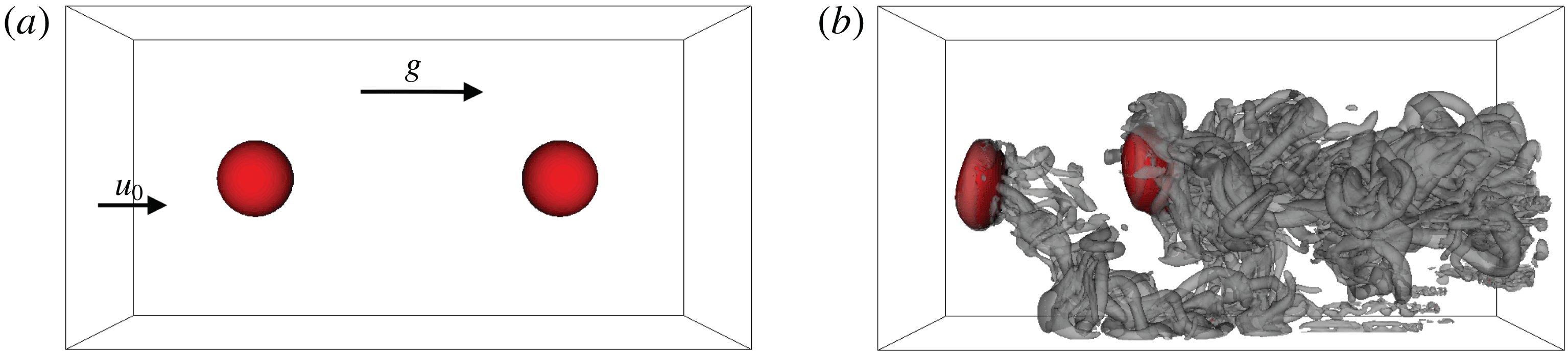
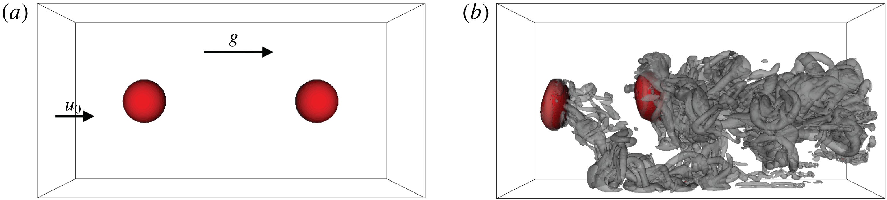
Three-dimensional inflow–outflow DNS configuration: red bubble surface and semi-transparent grey
 $Q=10$
isocontour for the initial state (a) and the analysed snapshot of case A (b). Inflow velocity
 $\boldsymbol{u}_{0}$
and gravitational acceleration
 $\boldsymbol{g}$
are oriented from left to right.
Characterized by a high density and viscosity ratio, as well as comparably strong surface-tension forces, two air bubbles, featuring an initial diameter of
 $D_{b}=5$
mm, are suspended in a continuous water medium. A counterflow set-up, as displayed in figure 1, is chosen in accordance with a similar experimental configuration by Haase et al. (Reference Haase, Kück, Thöming and Kähler2017). (For layout purposes, all figures directly visualizing the flow are rotated in the following, i.e. the mean flow and the gravitational force are oriented from left to right.) Likewise, the set-up is similar to a DNS study of Toutant et al. (Reference Toutant, Labourasse, Lebaigue and Simonin2008), which aimed at the interaction between a deformable bubble and spatially decaying turbulence. In contrast to small bubbles (
 $D_{b}<1$
mm), for which surface-tension effects are dominant, the large bubbles investigated here imply strong interface deformations. The separation distance of the two bubbles was
 $4D_{b}$
initially, but decreases during the course of the simulation. Such entrainment effects of two ellipsoidal bubbles in counterflow have been confirmed experimentally by Brücker (Reference Brücker1999). The idea behind the two-bubble configuration was to allow a simultaneous observation of the differences in the behaviour of the leading bubble directly facing the laminar flow from the inlet, and the succeeding bubble facing the turbulent wake of the leading bubble. A higher number of bubbles would increase the complexity unnecessarily. The constant inflow velocity of
 $u_{0}=18.5~\text{cm}~\text{s}^{-1}$
roughly corresponds to the terminal velocity of a freely rising bubble in a globally stagnant flow, and therefore limits the length of the three-dimensional computational domain (
 $40~\text{mm}\times 20~\text{mm}\times 20~\text{mm}$
). Koebe et al. (Reference Koebe, Bothe, Pruess and Warnecke2002) demonstrated that a wall distance of four bubble diameters together with slip boundary conditions was sufficient to compute the correct rise velocity of a single bubble rising without wall influence. Owing to the bubble Reynolds number of
 $Re_{b}=u_{0}D_{b}/\unicode[STIX]{x1D708}_{l}=921.5$
, wobbling ellipsoidal bubbles are observed in the simulations, which is in agreement with the Grace regime diagram (Clift, Grace & Weber Reference Clift, Grace and Weber2005). Since
 $Re_{b}$
is based on the fluid properties of the liquid phase, it is unaffected by the gas-phase modifications discussed later. At the boundaries of the domain, classical inflow/outflow conditions are combined with slip conditions at the channel sidewalls (for reasons of numerical robustness amongst others). Periodic boundary conditions in the axial direction were avoided because the bubbles would be facing their own turbulent wake from the inlet in this case.
Meshing by a uniform Cartesian grid yields
 $D_{b}/\unicode[STIX]{x0394}x=40$
, which is assumed to be a sufficiently high resolution of the bubble, as discussed in the following. According to Koebe, Bothe & Warnecke (Reference Koebe, Bothe and Warnecke2003), there is hardly any difference in terms of the rise velocity between 16 and 32 cells per bubble diameter. The bubble Weber number
 $We=\unicode[STIX]{x1D70C}_{l}u_{0}^{2}D_{b}/\unicode[STIX]{x1D70E}$
and the grid Weber number
 $We_{\unicode[STIX]{x0394}x}=\unicode[STIX]{x1D70C}_{l}u_{0}^{2}\unicode[STIX]{x0394}x/\unicode[STIX]{x1D70E}$
can be calculated to be 2.348 and 0.059, respectively. The latter value is sometimes applied in the literature, as can be seen in Desjardins & Pitsch (Reference Desjardins and Pitsch2010), to evaluate the grid spacing with respect to droplet stability resolution requirements. The value of
 $We_{\unicode[STIX]{x0394}x}$
achieved here is far smaller than the critical value of 10. Bubble breakup, bubble coalescence and other complex phenomena are not investigated here. According to the universal equilibrium theory by Kolmogorov, the smallest dissipative length scale that has to be resolved for the DNS can be estimated by
 $\unicode[STIX]{x1D702}\approx L_{t}Re_{t}^{-3/4}$
using the integral turbulent length scale
 $L_{t}$
and the turbulent Reynolds number
 $Re_{t}=u^{\prime }L_{t}/\unicode[STIX]{x1D708}_{l}$
(Batchelor Reference Batchelor1953). Assuming, in a conservative manner, that
 $Re_{t}=Re_{b}$
and
 $L_{t}=D_{b}$
yields
 $\unicode[STIX]{x1D702}\approx 29.9~\unicode[STIX]{x03BC}\text{m}$
. Alternatively, one may estimate
 $\unicode[STIX]{x1D716}\approx u_{0}g$
(Koebe et al.
Reference Koebe, Bothe and Warnecke2003) and use
 $\unicode[STIX]{x1D708}=\unicode[STIX]{x1D708}_{l}$
to obtain the Kolmogorov length scale
 $\unicode[STIX]{x1D702}=(\unicode[STIX]{x1D708}^{3}/\unicode[STIX]{x1D716})^{1/4}\approx 27.3~\unicode[STIX]{x03BC}\text{m}$
. The achieved grid spacing is of the same order of magnitude as
 $\unicode[STIX]{x1D702}$
and therefore can be considered sufficient for the evaluation of first- and second-order statistics (Grötzbach Reference Grötzbach2011).
Spanning at least 10 bubble overflow times, the simulation duration is comparable in all cases, except when analysing the time history of bubble entrainment in case A. Visualizing an isosurface of the second invariant
 $Q$
(defined in § 3), figure 1(b) gives an impression of the highly unsteady, irregular and three-dimensional vortex structures in the wake of the wobbling bubbles.
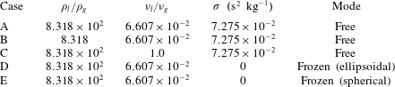
DNS case overview in terms of liquid-to-gas density ratio
 $\unicode[STIX]{x1D70C}_{l}/\unicode[STIX]{x1D70C}_{g}$
, kinematic viscosity ratio
 $\unicode[STIX]{x1D708}_{l}/\unicode[STIX]{x1D708}_{g}$
, surface tension
 $\unicode[STIX]{x1D70E}$
and mode of bubble motion.
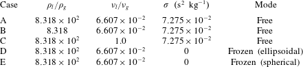
An overview of the examined cases is provided in table 1. Only the reference case, case A, agrees with the physical reality in terms of the fluid properties and the degrees of freedom of bubble motion. All other cases might be characterized as ‘numerical experiments’. In the sense of the process of elimination, specific parameters of the problem are manipulated successively to exclude or minimize their influence on the observed phenomena, which will subsequently be explained. The gas density and viscosity, and consequently the liquid-to-gas ratios, are adjusted in the cases B and C, respectively. For the cases D and E, the surface-tension forces are switched off. This is only possible for frozen bubble shapes, as the bubbles would disintegrate immediately otherwise. From a technical point of view, the update of the volume fraction field (equation (2.1)) is stopped at two different points in time, resulting in two different frozen bubble shapes: ellipsoidal versus spherical. Hence, the density and viscosity field are kept constant and the capillary pressure jump vanishes when the simulation is continued.
3 Mathematical background
According to Perry & Chong (Reference Perry and Chong1987) and Chong et al. (Reference Chong, Perry and Cantwell1990), amongst others, the invariants of the velocity-gradient tensor
 $\unicode[STIX]{x1D608}_{ij}=\unicode[STIX]{x2202}u_{i}/\unicode[STIX]{x2202}x_{j}=\unicode[STIX]{x1D61A}_{ij}+\unicode[STIX]{x1D61E}_{ij}$
give rise to a set of local flow topologies. Here,
 $\unicode[STIX]{x1D61A}_{ij}=0.5(\unicode[STIX]{x1D608}_{ij}+\unicode[STIX]{x1D608}_{ji})$
and
 $\unicode[STIX]{x1D61E}_{ij}=0.5(\unicode[STIX]{x1D608}_{ij}-\unicode[STIX]{x1D608}_{ji})$
represent the tensor’s symmetric and antisymmetric components, respectively. The corresponding characteristic equation is given by
 $\unicode[STIX]{x1D706}^{3}+P\unicode[STIX]{x1D706}^{2}+Q\unicode[STIX]{x1D706}+R=0$
, with
 $$\begin{eqnarray}\displaystyle & P=-\unicode[STIX]{x1D61A}_{ii}=-(\unicode[STIX]{x1D706}_{1}+\unicode[STIX]{x1D706}_{2}+\unicode[STIX]{x1D706}_{3}), & \displaystyle\end{eqnarray}$$
 $$\begin{eqnarray}\displaystyle & Q=(P^{2}-\unicode[STIX]{x1D61A}_{ij}\unicode[STIX]{x1D61A}_{ij}+\unicode[STIX]{x1D61E}_{ij}\unicode[STIX]{x1D61E}_{ij})/2, & \displaystyle\end{eqnarray}$$
 $$\begin{eqnarray}\displaystyle & R=(-P^{3}+3PQ-\unicode[STIX]{x1D61A}_{ij}\unicode[STIX]{x1D61A}_{jk}\unicode[STIX]{x1D61A}_{ki}-3\unicode[STIX]{x1D61E}_{ij}\unicode[STIX]{x1D61E}_{jk}\unicode[STIX]{x1D61A}_{ki})/3, & \displaystyle\end{eqnarray}$$
being the invariants of
 $\unicode[STIX]{x1D608}_{ij}$
, and exhibiting three solutions, i.e. the eigenvalues
 $\unicode[STIX]{x1D706}_{1}$
,
 $\unicode[STIX]{x1D706}_{2}$
and
 $\unicode[STIX]{x1D706}_{3}$
of
 $\unicode[STIX]{x1D608}_{ij}$
. The characteristic equation’s discriminant
 $D=(27R^{2}+(4P^{3}-18PQ)R+4Q^{3}-P^{2}Q^{2})/108$
divides the
 $P$
–
 $Q$
–
 $R$
phase space into two regions:
(i)
 $D>0$
, where
$\unicode[STIX]{x1D608}_{ij}$
shows one real eigenvalue and two complex conjugate eigen-values, and therefore focal topologies; and
(ii)
$D<0$
, where
$\unicode[STIX]{x1D608}_{ij}$
shows three real eigenvalues, and therefore nodal topologies.


Corresponding to
 $D=0$
, two surfaces separating the topologies in the phase space are given by
 $r_{1a}=P(Q-2P^{2}/9)/3-2(-3Q+P^{2})^{3/2}/27$
and
 $r_{1b}=P(Q-2P^{2}/9)/3+2(-3Q+P^{2})^{3/2}/27$
. In the region
 $D>0$
,
 $\unicode[STIX]{x1D608}_{ij}$
has purely imaginary eigenvalues on the surface
 $r_{2}=PQ$
. The surfaces
 $r_{1a}$
,
 $r_{1b}$
and
 $r_{2}$
divide the
 $P$
–
 $Q$
–
 $R$
phase space into eight flow topologies in the general case.
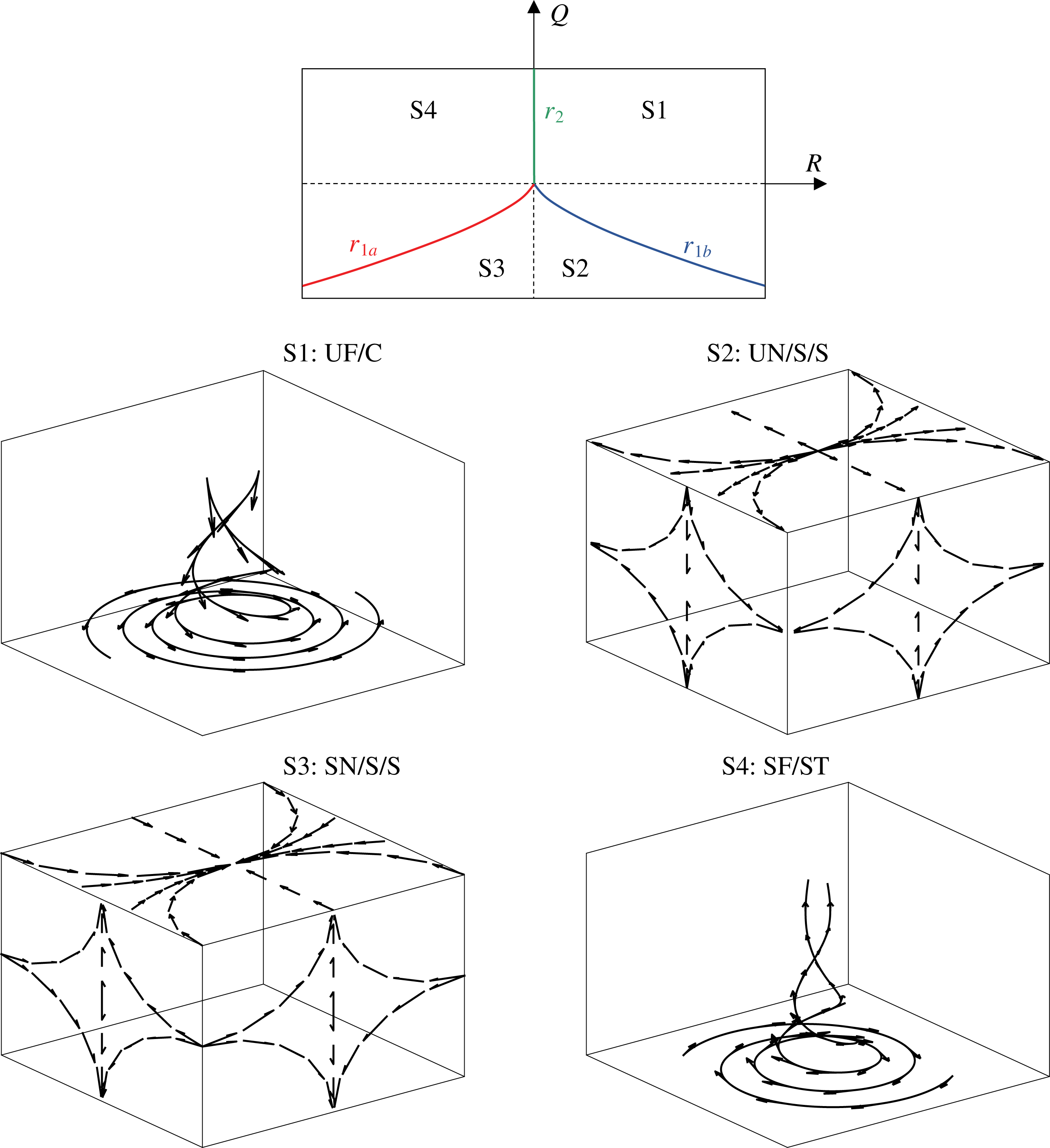
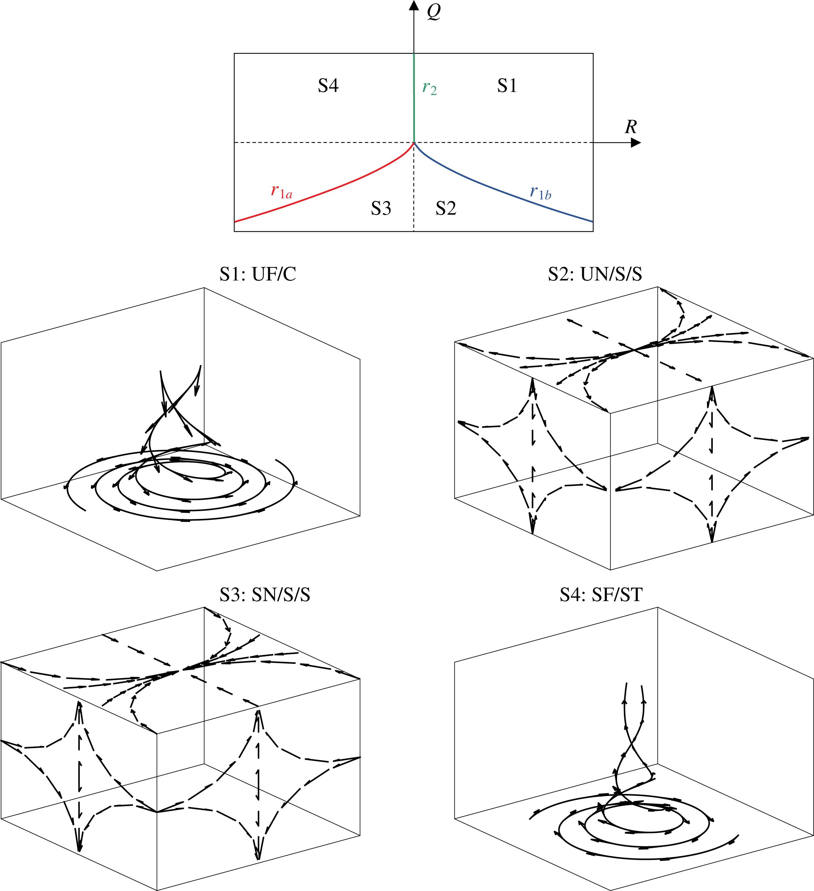
Classification of topologies S1–S4 (top): projection of topology borders
 $r_{1a}$
,
 $r_{1b}$
and
 $r_{2}$
in the
 $Q$
–
 $R$
plane for
 $P=0$
. Dashed lines indicate
 $Q=0$
and
 $R=0$
, respectively. Graphical representation (bottom), corresponding to UF
 $=$
unstable focus, UN
 $=$
unstable node, SN
 $=$
stable node, SF
 $=$
stable focus, C
 $=$
compressing, S
 $=$
saddle, ST
 $=$
stretching.
For incompressible fluids, the three-dimensional
 $P$
–
 $Q$
–
 $R$
phase space is reduced to the two-dimensional
 $Q$
–
 $R$
phase space since
 $P=-\unicode[STIX]{x1D735}\boldsymbol{\cdot }\boldsymbol{u}=0$
. The number of flow topologies is consequently reduced from eight to four. Both the topology borders
 $r_{1a}$
,
 $r_{1b}$
and
 $r_{2}$
in the
 $Q$
–
 $R$
phase space, as well as a graphical representation of topologies S1–S4, are shown in figure 2. To simplify the interpretation, the second invariant of
 $\unicode[STIX]{x1D608}_{ij}$
,
 $Q$
, can be split into two parts:
 $$\begin{eqnarray}Q=Q_{S}+Q_{W}=-\unicode[STIX]{x1D61A}_{ij}\unicode[STIX]{x1D61A}_{ij}/2+\unicode[STIX]{x1D61E}_{ij}\unicode[STIX]{x1D61E}_{ij}/2,\end{eqnarray}$$
where
 $Q_{S}$
and
 $Q_{W}$
denote the second invariant of
 $\unicode[STIX]{x1D61A}_{ij}$
and
 $\unicode[STIX]{x1D61E}_{ij}$
, respectively. The latter part
 $Q_{W}$
is directly related to vorticity
 $\unicode[STIX]{x1D74E}$
and enstrophy
 $\unicode[STIX]{x1D6FA}$
according to
 $$\begin{eqnarray}\unicode[STIX]{x1D61E}_{ij}\unicode[STIX]{x1D61E}_{ij}/2=\unicode[STIX]{x1D714}_{i}\unicode[STIX]{x1D714}_{i}/4=\unicode[STIX]{x1D6FA}/2.\end{eqnarray}$$
Thus,
 $Q<0$
is indicative of strain-dominated regions and
 $Q>0$
is indicative of vorticity-dominated regions. In a similar manner, the expression of the third invariant
 $R$
may be restated as
 $$\begin{eqnarray}R=R_{S}-\unicode[STIX]{x1D61E}_{ij}\unicode[STIX]{x1D61E}_{jk}\unicode[STIX]{x1D61A}_{ki}=-\unicode[STIX]{x1D61A}_{ij}\unicode[STIX]{x1D61A}_{jk}\unicode[STIX]{x1D61A}_{ki}/3-\unicode[STIX]{x1D61E}_{ij}\unicode[STIX]{x1D61E}_{jk}\unicode[STIX]{x1D61A}_{ki},\end{eqnarray}$$
where
 $R_{S}$
is the third invariant of the strain-rate tensor
 $\unicode[STIX]{x1D61A}_{ij}$
. The second term on the right-hand side (without the negative sign) could be linked to the vortex-stretching term of the enstrophy transport equation (Tsinober Reference Tsinober2000). Owing to their prominent roles, the isosurfaces specified by
 $Q=0$
and
 $R=0$
are included in the subsequent invariant plots.
To compute the velocity vector
 $\boldsymbol{u}$
, the momentum balance equation for two-phase flows can generally be written as
 $$\begin{eqnarray}\frac{\text{D}u_{i}}{\text{D}t}\equiv \frac{\unicode[STIX]{x2202}u_{i}}{\unicode[STIX]{x2202}t}+u_{j}\frac{\unicode[STIX]{x2202}u_{i}}{\unicode[STIX]{x2202}x_{j}}=-\frac{1}{\unicode[STIX]{x1D70C}}\frac{\unicode[STIX]{x2202}p}{\unicode[STIX]{x2202}x_{i}}+\frac{1}{\unicode[STIX]{x1D70C}}\frac{\unicode[STIX]{x2202}\unicode[STIX]{x1D70F}_{ij}}{\unicode[STIX]{x2202}x_{j}}+g_{i}+\frac{1}{\unicode[STIX]{x1D70C}}\unicode[STIX]{x1D70E}\unicode[STIX]{x1D705}n_{i}\unicode[STIX]{x1D6FF}_{S},\end{eqnarray}$$
in which the interface Dirac function
 $\unicode[STIX]{x1D6FF}_{S}\equiv \unicode[STIX]{x1D6FF}(\boldsymbol{x}-\boldsymbol{x}_{S})$
is approximated by
 $|\unicode[STIX]{x1D735}\unicode[STIX]{x1D6FC}|$
, and thus
 $\boldsymbol{n}\unicode[STIX]{x1D6FF}_{S}=-\unicode[STIX]{x1D735}\unicode[STIX]{x1D6FC}$
, according to the continuum surface force (CSF) methodology as proposed by Brackbill, Kothe & Zemach (Reference Brackbill, Kothe and Zemach1992). The quantities
 $\unicode[STIX]{x1D70E}$
,
 $\unicode[STIX]{x1D705}$
and
 $\boldsymbol{n}=-\unicode[STIX]{x1D735}\unicode[STIX]{x1D6FC}/|\unicode[STIX]{x1D735}\unicode[STIX]{x1D6FC}|$
denote the surface tension, the interface mean curvature and the interface normal vector, respectively. The viscous stress tensor
 $\unicode[STIX]{x1D70F}_{ij}$
is formulated on the basis of Stokes’ hypothesis, which reduces to
 $$\begin{eqnarray}\unicode[STIX]{x1D70F}_{ij}=\unicode[STIX]{x1D707}\left(\frac{\unicode[STIX]{x2202}u_{i}}{\unicode[STIX]{x2202}x_{j}}+\frac{\unicode[STIX]{x2202}u_{j}}{\unicode[STIX]{x2202}x_{i}}-\frac{2}{3}\unicode[STIX]{x1D6FF}_{ij}\frac{\unicode[STIX]{x2202}u_{m}}{\unicode[STIX]{x2202}x_{m}}\right)=\unicode[STIX]{x1D707}\left(\frac{\unicode[STIX]{x2202}u_{i}}{\unicode[STIX]{x2202}x_{j}}+\frac{\unicode[STIX]{x2202}u_{j}}{\unicode[STIX]{x2202}x_{i}}\right)\end{eqnarray}$$
for incompressible flows (
 $\unicode[STIX]{x1D735}\boldsymbol{\cdot }\boldsymbol{u}=0$
).
An evolution equation for the vorticity
 $\unicode[STIX]{x1D74E}\equiv \unicode[STIX]{x1D735}\times \boldsymbol{u}$
can be derived by taking the curl of (3.7) (
 $e_{ijk}$
stands for the Levi-Civita symbol):
 $$\begin{eqnarray}\frac{\text{D}\unicode[STIX]{x1D714}_{i}}{\text{D}t}=-\underbrace{\unicode[STIX]{x1D714}_{i}\frac{\unicode[STIX]{x2202}u_{j}}{\unicode[STIX]{x2202}x_{j}}}_{T_{1}}+\underbrace{\unicode[STIX]{x1D714}_{j}\frac{\unicode[STIX]{x2202}u_{i}}{\unicode[STIX]{x2202}x_{j}}}_{T_{2}}-\underbrace{\frac{e_{ijk}}{\unicode[STIX]{x1D70C}^{2}}\frac{\unicode[STIX]{x2202}\unicode[STIX]{x1D70C}}{\unicode[STIX]{x2202}x_{j}}\frac{\unicode[STIX]{x2202}\unicode[STIX]{x1D70F}_{km}}{\unicode[STIX]{x2202}x_{m}}}_{T_{31}}+\underbrace{\frac{e_{ijk}}{\unicode[STIX]{x1D70C}}\frac{\unicode[STIX]{x2202}^{2}\unicode[STIX]{x1D70F}_{km}}{\unicode[STIX]{x2202}x_{j}\unicode[STIX]{x2202}x_{m}}}_{T_{32}}+\underbrace{\frac{e_{ijk}}{\unicode[STIX]{x1D70C}^{2}}\frac{\unicode[STIX]{x2202}\unicode[STIX]{x1D70C}}{\unicode[STIX]{x2202}x_{j}}\frac{\unicode[STIX]{x2202}p}{\unicode[STIX]{x2202}x_{k}}}_{T_{4}}+\,T_{5}.\end{eqnarray}$$
In the order given, the terms on the right-hand side of (3.9) represent the following:
(i)
$T_{1}$
= vorticity destruction by dilatation rate;(ii)
$T_{2}$
= vortex stretching;(iii)
$T_{31}$
= misalignment between the gradients of density and viscous stress;(iv)
$T_{32}$
= viscous diffusion and dissipation of vorticity;(v)
$T_{4}$
= baroclinic effects arising from the misalignment of density and pressure gradients;(vi)
$T_{5}$
= effects related to the surface tension.


Term
 $T_{1}$
vanishes for incompressible flows. Regarding term
 $T_{4}$
, it should be mentioned that the pressure gradient resulting from the capillary pressure jump (
 $\unicode[STIX]{x0394}p\sim \unicode[STIX]{x1D70E}\unicode[STIX]{x1D705}$
) alone would be theoretically aligned with the density gradient at the interface. However, dynamic pressure variations in the flow can lead to a misalignment of both gradients and consequently give rise to vorticity deposition at the interface. Compared to single-phase flows, another potential vorticity production term occurs due to the capillary force itself,
 $$\begin{eqnarray}T_{5}=\underbrace{e_{ijk}\frac{\unicode[STIX]{x1D70E}}{\unicode[STIX]{x1D70C}^{2}}\frac{\unicode[STIX]{x2202}\unicode[STIX]{x1D70C}}{\unicode[STIX]{x2202}x_{j}}\frac{\unicode[STIX]{x2202}\unicode[STIX]{x1D6FC}}{\unicode[STIX]{x2202}x_{k}}\unicode[STIX]{x1D705}}_{T_{51}}-\underbrace{e_{ijk}\frac{\unicode[STIX]{x1D70E}}{\unicode[STIX]{x1D70C}}\frac{\unicode[STIX]{x2202}^{2}\unicode[STIX]{x1D6FC}}{\unicode[STIX]{x2202}x_{j}\unicode[STIX]{x2202}x_{k}}\unicode[STIX]{x1D705}}_{T_{52}}-\underbrace{e_{ijk}\frac{\unicode[STIX]{x1D70E}}{\unicode[STIX]{x1D70C}}\frac{\unicode[STIX]{x2202}\unicode[STIX]{x1D6FC}}{\unicode[STIX]{x2202}x_{k}}\frac{\unicode[STIX]{x2202}\unicode[STIX]{x1D705}}{\unicode[STIX]{x2202}x_{j}}}_{T_{53}},\end{eqnarray}$$
with the interface mean curvature generally given by
 $$\begin{eqnarray}\unicode[STIX]{x1D705}=\frac{\unicode[STIX]{x2202}n_{j}}{\unicode[STIX]{x2202}x_{j}}=-\frac{1}{|\unicode[STIX]{x1D735}\unicode[STIX]{x1D6FC}|}\frac{\unicode[STIX]{x2202}^{2}\unicode[STIX]{x1D6FC}}{\unicode[STIX]{x2202}x_{j}\unicode[STIX]{x2202}x_{j}}+\frac{1}{|\unicode[STIX]{x1D735}\unicode[STIX]{x1D6FC}|^{2}}\frac{\unicode[STIX]{x2202}|\unicode[STIX]{x1D735}\unicode[STIX]{x1D6FC}|}{\unicode[STIX]{x2202}x_{j}}\frac{\unicode[STIX]{x2202}\unicode[STIX]{x1D6FC}}{\unicode[STIX]{x2202}x_{j}}.\end{eqnarray}$$
Term
 $T_{51}$
vanishes since
 $\unicode[STIX]{x1D735}\unicode[STIX]{x1D70C}=(\unicode[STIX]{x1D70C}_{g}-\unicode[STIX]{x1D70C}_{l})\unicode[STIX]{x1D735}\unicode[STIX]{x1D6FC}\propto \unicode[STIX]{x1D735}\unicode[STIX]{x1D6FC}$
, according to (2.2) and
 $\unicode[STIX]{x1D735}\unicode[STIX]{x1D6FC}\times \unicode[STIX]{x1D735}\unicode[STIX]{x1D6FC}=0$
(i.e. absence of misalignment). Term
 $T_{52}$
is equal to zero, since the curl of gradients vanishes,
 $\unicode[STIX]{x1D735}\times (\unicode[STIX]{x1D735}\unicode[STIX]{x1D6FC})=0$
. Similarly, the conservative gravitational force does not affect the vorticity field and hence does not appear in (3.9). Interestingly, the remaining term
 $T_{53}$
does not scale with density gradients, unlike the other relevant production terms of (3.9). Regarding the geometric interpretation of term
 $T_{53}$
, it is instructive to think in terms of interface-normal (subscript
 $n$
) and interface-tangential (subscript
 $t$
) components of
 $\unicode[STIX]{x1D735}\unicode[STIX]{x1D6FC}$
and
 $\unicode[STIX]{x1D735}\unicode[STIX]{x1D705}$
. Since
 $\unicode[STIX]{x1D735}_{\!t}\,\unicode[STIX]{x1D6FC}=0$
, the non-zero contribution of
 $\unicode[STIX]{x1D735}\unicode[STIX]{x1D705}\times \unicode[STIX]{x1D735}\unicode[STIX]{x1D6FC}$
arises from the perpendicular vectors
 $\unicode[STIX]{x1D735}_{\!n}\,\unicode[STIX]{x1D6FC}$
and
 $\unicode[STIX]{x1D735}_{\!t}\,\unicode[STIX]{x1D705}$
. Term
 $T_{53}$
gains in importance for (heavily) deformed bubbles as
 $\unicode[STIX]{x1D735}_{\!t}\,\unicode[STIX]{x1D705}=0$
, and thus
 $T_{53}=0$
for perfectly spherical bubbles.
In the following analysis, a direct quantitative evaluation of these terms, particularly for term
 $T_{5}$
, has not been conducted, as the calculation of third-order derivatives of the discrete representation of a discontinuous function (
 $\unicode[STIX]{x1D6FC}$
here) is extremely challenging from a numerical point of view. For the aforementioned reasons, an indirect assessment is preferred instead.
4 Analytical solution
Although turbulent flows cannot be described by the analytical creeping-flow solution of Hadamard and Rybczynski (Clift et al. Reference Clift, Grace and Weber2005; Sadhal, Ayyaswamy & Chung Reference Sadhal, Ayyaswamy and Chung2012), it is still discussed here, as it offers insights into the understanding of bubble-affected flows. The solution strictly holds only for inertialess spherical bubbles at a very low Reynolds number. An extension that accounts for inertia effects and small interface deformation is given by Taylor & Acrivos (Reference Taylor and Acrivos1964), but this does not provide significant further insights in the context of this work. It is important to mention that the streamfunction-based analytical solution by Hadamard and Rybczynski does not represent a potential flow, which is irrotational by definition.
Starting from the general ansatz
 $$\begin{eqnarray}\unicode[STIX]{x1D713}=\sin ^{2}(\unicode[STIX]{x1D703})\left(\frac{A}{r}+Br+Cr^{2}+Dr^{4}\right)\end{eqnarray}$$
for the Stokes streamfunction of both phases, eight constants (
 $A,B,C,D$
, all
 $\times 2$
) need to be determined. This can be achieved by requiring continuity at the interface in terms of normal velocity, tangential velocity, shear stress and normal stress, along with the corresponding conditions in the far field. Since the solution is axisymmetric with respect to the axis pointing in the mean flow direction, there is a dependence not on azimuthal direction
 $\unicode[STIX]{x1D711}$
, but on radius
 $r$
and inclination
 $\unicode[STIX]{x1D703}$
in spherical coordinates. The velocity components can then be obtained from
 $$\begin{eqnarray}u_{r}=\frac{1}{r^{2}\sin \unicode[STIX]{x1D703}}\frac{\unicode[STIX]{x2202}\unicode[STIX]{x1D713}}{\unicode[STIX]{x2202}\unicode[STIX]{x1D703}}\end{eqnarray}$$
for the radial direction, and
 $$\begin{eqnarray}u_{\unicode[STIX]{x1D703}}=-\frac{1}{r\sin \unicode[STIX]{x1D703}}\frac{\unicode[STIX]{x2202}\unicode[STIX]{x1D713}}{\unicode[STIX]{x2202}r}\end{eqnarray}$$
for the circumferential direction.
Given the unperturbed inflow velocity
 $u_{0}$
, bubble radius
 $R_{b}$
and dynamic viscosity ratio
 $\unicode[STIX]{x1D719}=\unicode[STIX]{x1D707}_{g}/\unicode[STIX]{x1D707}_{l}$
, the streamfunctions
 $\unicode[STIX]{x1D713}$
of the liquid and gaseous phases finally read
 $$\begin{eqnarray}\unicode[STIX]{x1D713}_{l}(r,\unicode[STIX]{x1D703})=-\frac{1}{2}u_{0}R_{b}^{2}\sin ^{2}(\unicode[STIX]{x1D703})\left[\left(\frac{r}{R_{b}}\right)^{2}-\left(\frac{2+3\unicode[STIX]{x1D719}}{2(1+\unicode[STIX]{x1D719})}\right)\left(\frac{r}{R_{b}}\right)+\left(\frac{\unicode[STIX]{x1D719}}{2(1+\unicode[STIX]{x1D719})}\right)\left(\frac{R_{b}}{r}\right)\right]\end{eqnarray}$$
and
 $$\begin{eqnarray}\unicode[STIX]{x1D713}_{g}(r,\unicode[STIX]{x1D703})=\frac{1}{4}u_{0}R_{b}^{2}\sin ^{2}(\unicode[STIX]{x1D703})\left(\frac{1}{1+\unicode[STIX]{x1D719}}\right)\left[\left(\frac{r}{R_{b}}\right)^{2}-\left(\frac{r}{R_{b}}\right)^{4}\right],\end{eqnarray}$$
respectively.
Inserting (4.4) and (4.5) into the fundamental relation
 $$\begin{eqnarray}\unicode[STIX]{x1D714}(r,\unicode[STIX]{x1D703})=-\frac{1}{r\sin \unicode[STIX]{x1D703}}\left(\frac{\unicode[STIX]{x2202}^{2}\unicode[STIX]{x1D713}}{\unicode[STIX]{x2202}r^{2}}+\frac{\sin \unicode[STIX]{x1D703}}{r^{2}}\frac{\unicode[STIX]{x2202}}{\unicode[STIX]{x2202}\unicode[STIX]{x1D703}}\left(\frac{1}{\sin \unicode[STIX]{x1D703}}\frac{\unicode[STIX]{x2202}\unicode[STIX]{x1D713}}{\unicode[STIX]{x2202}\unicode[STIX]{x1D703}}\right)\right),\end{eqnarray}$$
where
 $\unicode[STIX]{x1D714}$
denotes the only non-zero component of
 $\unicode[STIX]{x1D74E}$
(perpendicular to the
 $r$
–
 $\unicode[STIX]{x1D703}$
plane), it can be derived, through reorganization and application of algebra, that the vorticity distribution in both phases is given by the comparably simple equations
 $$\begin{eqnarray}\displaystyle & \displaystyle \unicode[STIX]{x1D714}_{l}(r,\unicode[STIX]{x1D703})=u_{0}\frac{R_{b}}{r^{2}}\sin (\unicode[STIX]{x1D703})\left(\frac{2+3\unicode[STIX]{x1D719}}{2(1+\unicode[STIX]{x1D719})}\right), & \displaystyle\end{eqnarray}$$
 $$\begin{eqnarray}\displaystyle & \displaystyle \unicode[STIX]{x1D714}_{g}(r,\unicode[STIX]{x1D703})=\frac{5}{2}u_{0}\frac{r}{R_{b}^{2}}\sin (\unicode[STIX]{x1D703})\left(\frac{1}{1+\unicode[STIX]{x1D719}}\right). & \displaystyle\end{eqnarray}$$
Owing to the viscosity jump, the vorticity field is generally discontinuous at the interface (
 $r=R_{b}$
). Only if
 $\unicode[STIX]{x1D719}=1$
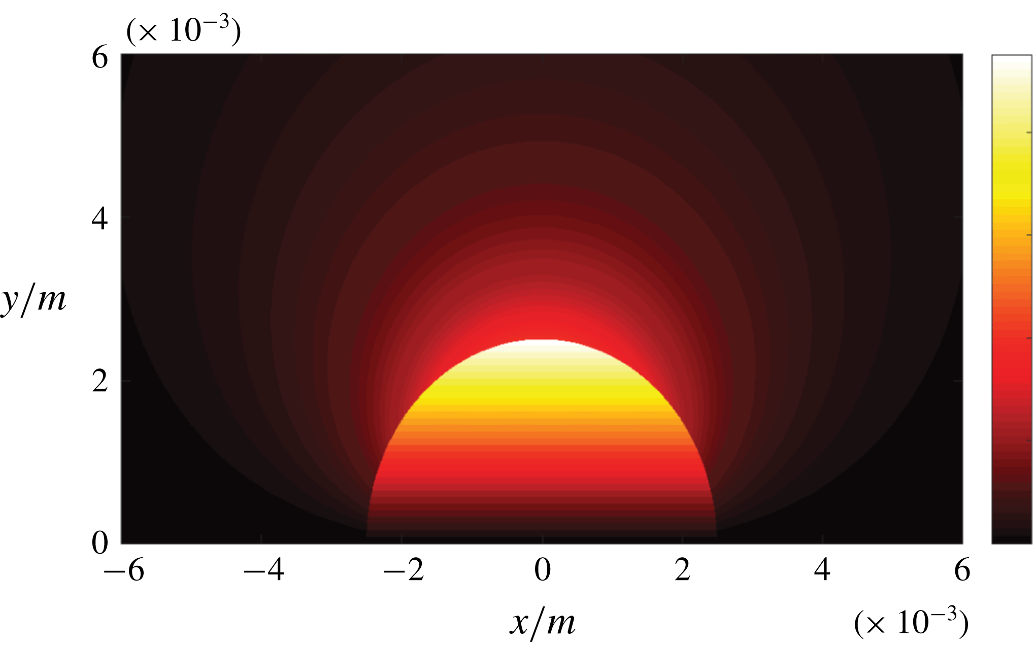
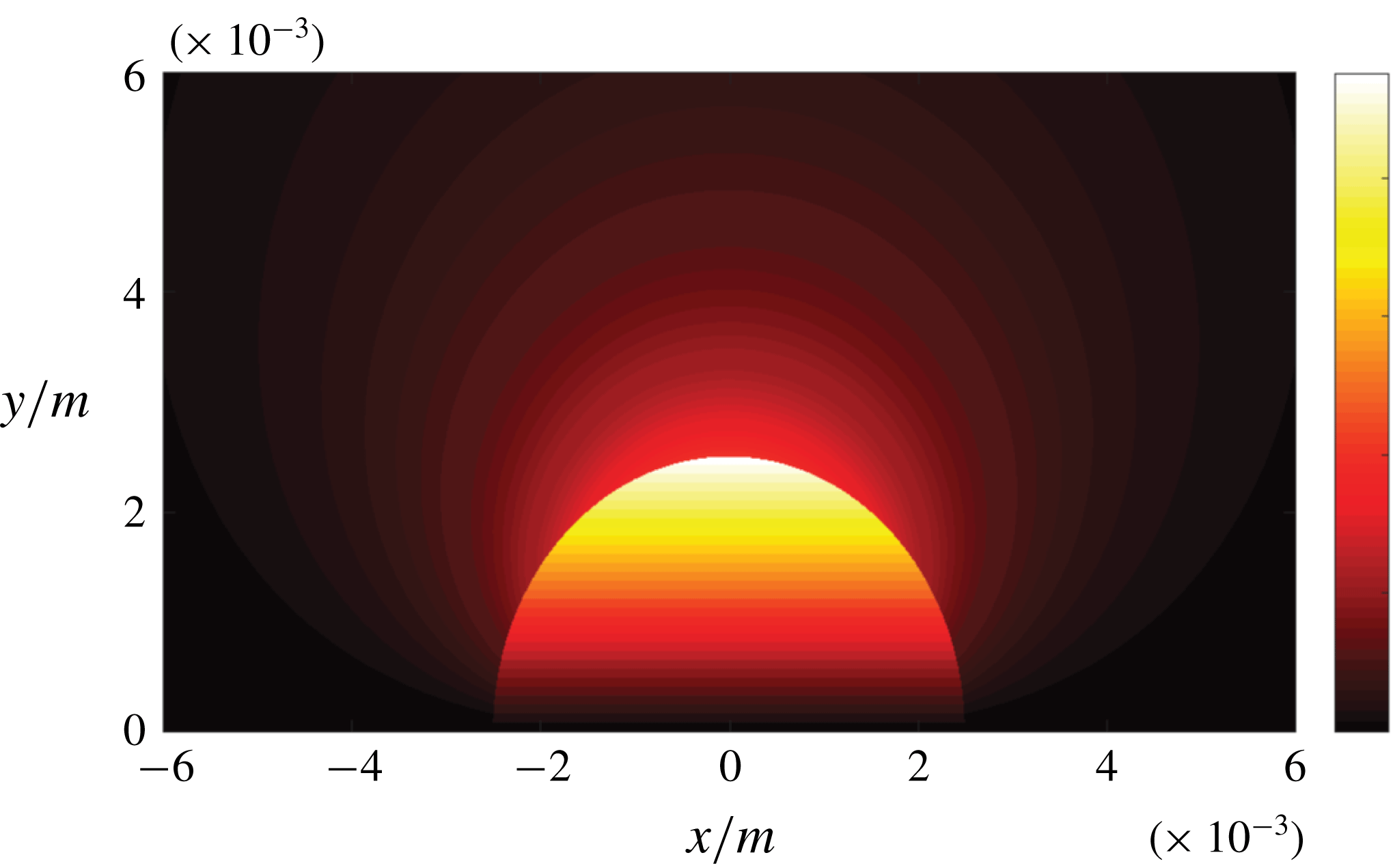
is the vorticity field continuous at the interface. As demonstrated in figure 3, the vorticity peaks at an inclination of
 $\unicode[STIX]{x1D703}=90^{\circ }$
and reaches zero at the symmetry axis. It should be noted that the bubble radius
 $R_{b}$
can be interpreted as an inverse measure of the interface curvature. When transferred to the situation studied numerically in the following (predominantly ellipsoidal bubbles), the vorticity is expected to reach the highest values at the regions involving simultaneously high fluid velocity and high interface curvature.
Analytical solution: axisymmetric vorticity field in the vicinity of the bubble; the mean flow direction is oriented from left to right.
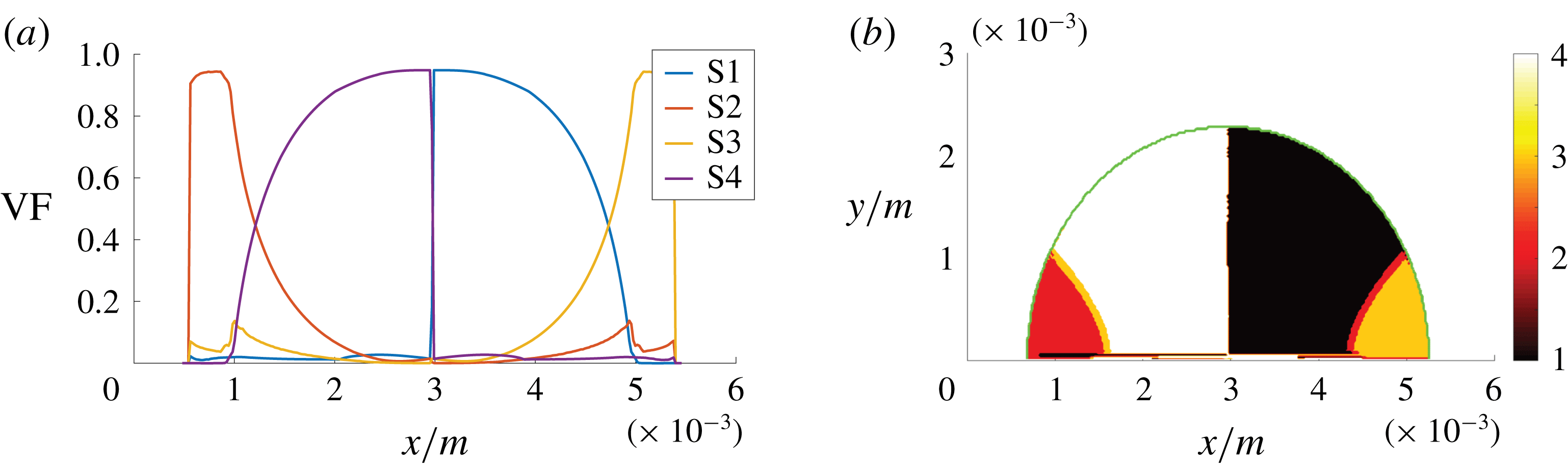
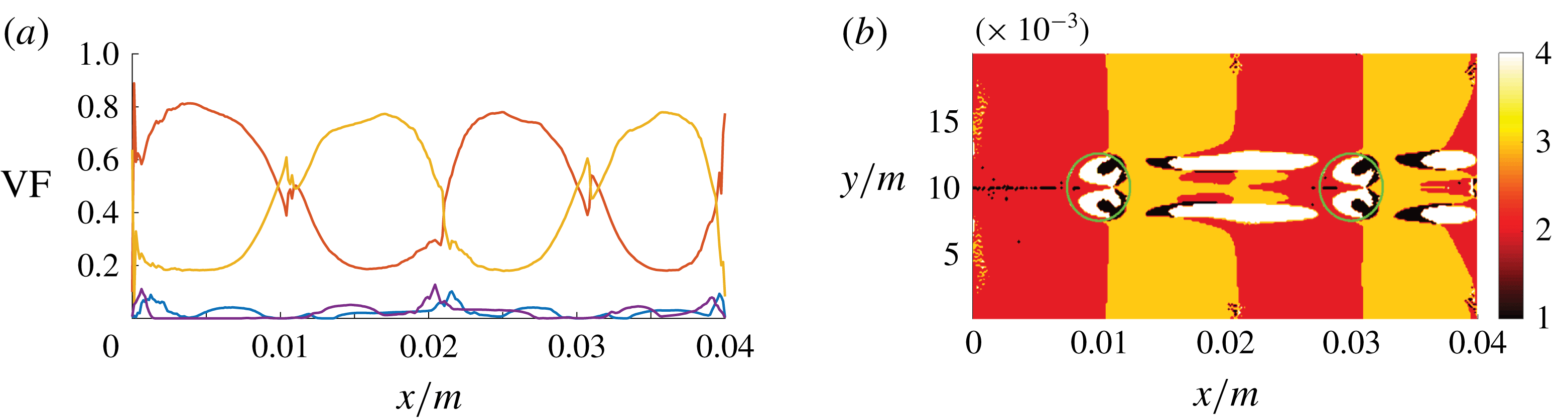
The semi-analytical solution, in terms of local flow topologies, is shown in figure 4. The solution is characterized as semi-analytical, since the underlying velocity field is analytical but the invariants analysis is performed with the same numerical tool as used for the DNS data. Only the bubble-interior gaseous flow is analysed here, as this is at the focus of interest for the interpretation of the subsequent (turbulent) simulations. Nodal topologies S2 and S3, and correspondingly focal topologies S4 and S1, can be observed in the upstream and downstream part of the bubble, respectively. According to their nature, focal topologies prevail in the high-vorticity region. It can be summarized that a nodal-to-focal-to-nodal transition occurs within the bubble. The narrow band of intermediate topologies, S3 in the upstream part of the bubble and S2 in the downstream part of the bubble, might be influenced by the finite resolution and machine accuracy.
Semi-analytical solution: axial volume fraction distribution of flow topologies for the gaseous phase (a) and corresponding topology field in the gaseous phase (b), where 1–4 in the colour bar refer to S1–S4, respectively. The green line indicates the phase interface; the mean flow direction is oriented from left to right.

The analytical solution is analysed at this juncture, as the comparison of different regimes of bubbly flows, namely the laminar creeping-flow solution versus turbulent DNS cases, provides additional insights, as will be shown in the following. On the one hand, striking similarities can be observed: the dominance of focal topologies in the gaseous phase and the switch from diverging flow topologies ahead of the bubble to converging flow topologies behind the bubble. On the other hand, some aspects are changing: regarding the jump of fluid properties at the interface, the dominant influence parameter, with respect to flow topologies, is the viscosity ratio in laminar flows but the density ratio is also important in turbulent flows.
5 Results and discussion
5.1 Case A (reference)
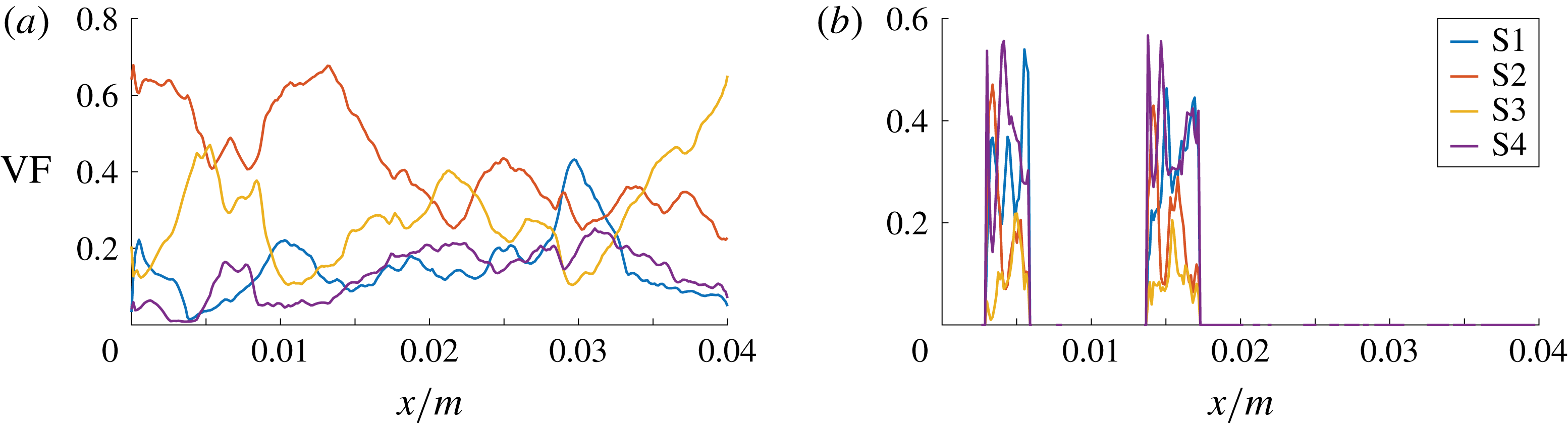
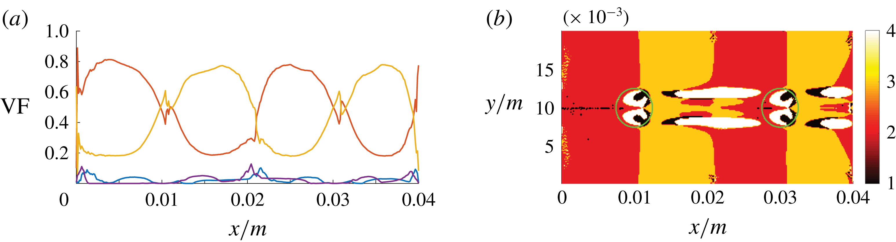
Case A agrees with the physical reality in terms of the fluid properties and the degrees of freedom of the bubble motion. It is used as a reference case that is compared with the cases involving the manipulation of the mathematical model. Figure 5 shows the axial volume fraction distribution of the flow topologies S1–S4, i.e. conditional averages (separately for the liquid and gaseous phases) with respect to both spanwise directions. The same approach has been adopted in subsequent similar figures, i.e. figures 11, 13 and 15. In the liquid phase, the level of focal topologies S1 and S4 is generally increasing in the downstream direction because of the turbulence induced by bubbles. Their location can be inferred from the corresponding plot of the gaseous phase. The non-zero volume fraction of focal topologies at the inlet boundary must be assessed as spurious behaviour, which stems from the ill-conditioned velocity gradient tensor at the laminar inflow. In terms of the nodal topologies, an exchange of topologies S2 and S3 seems to occur at the bubble locations. Case E is designed to explain that observation. In general, the situation in the liquid phase strongly depends on the analysed snapshot and the overall gas fraction in the domain, e.g. determined by the bubble size or number. In the gaseous phase, a different behaviour is observed. Although the kinematic viscosity is higher (
 $\unicode[STIX]{x1D708}_{g}>\unicode[STIX]{x1D708}_{l}$
) and, as such, the viscous damping is stronger, the level of focal topologies is clearly above the liquid phase. At the same time, there is no considerable difference between the first and second bubble.
DNS case A: axial volume fraction distribution of flow topologies for the liquid phase (a) and gaseous phase (b).
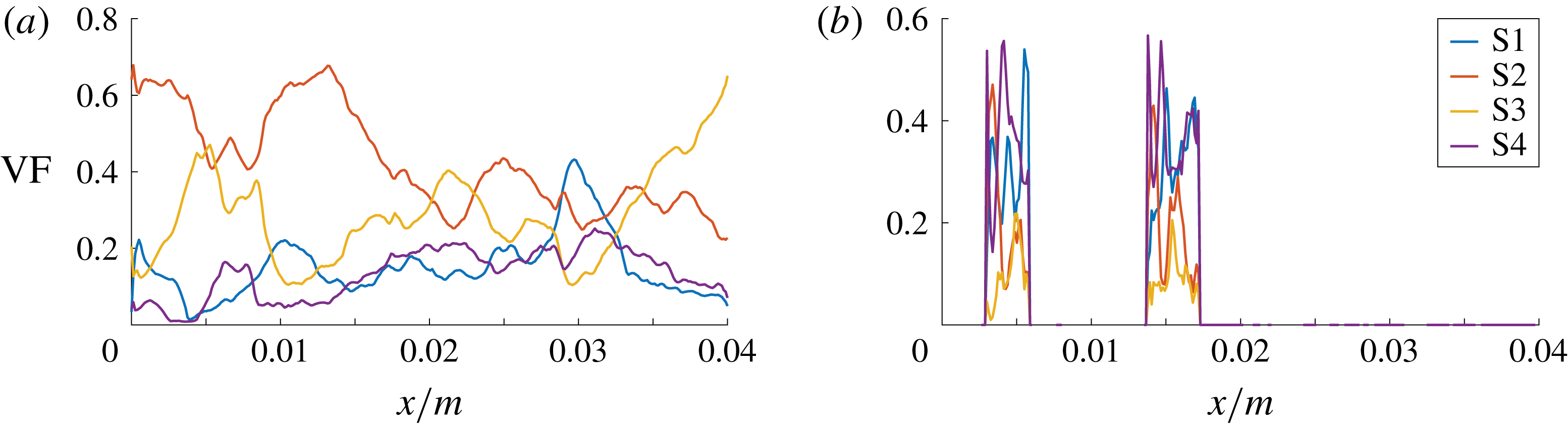
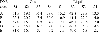
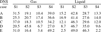
The axial distribution of topology volume fractions provides several insights, but the interpretation must be done with caution. The spanwise averages of the gaseous phase are particularly difficult to evaluate, since there is a clearly lower number of samples available at the front and rear part compared to the centre of the bubbles. Thus, the total percentage of topologies S1–S4, separately for the gaseous and liquid parts of the domain, is additionally given in table 2.
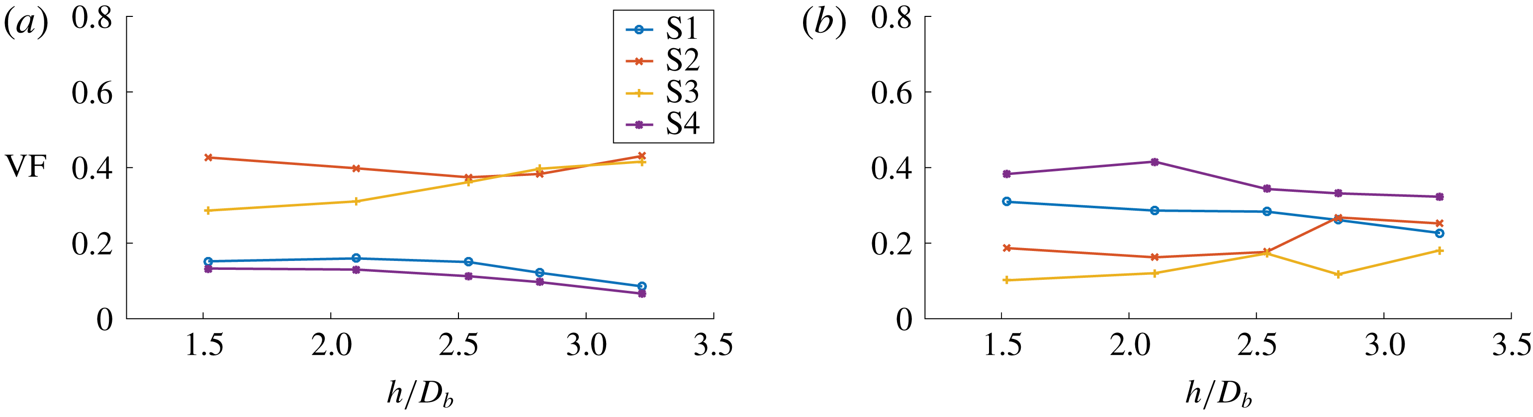
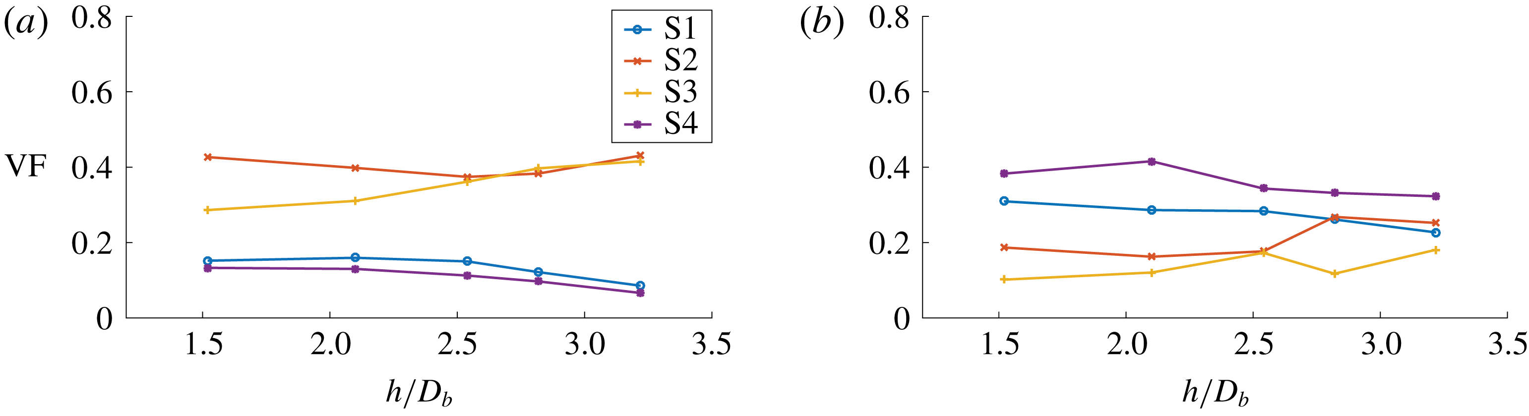
DNS case A: overall volume fraction of flow topologies for the liquid phase (a) and gaseous phase (b) during the bubble entrainment process, i.e. at different normalized bubble separation distances
 $h/D_{b}$
.
Total percentage of topologies S1–S4 in the gaseous and liquid parts of the domain for the analysed snapshot of each DNS case.
Owing to entrainment effects mentioned earlier, the second bubble is closing up with the first bubble compared to the initial condition (cf. figure 1). Figure 6 shows the overall topology volume fractions of both phases as a function of the bubble separation distance
 $h$
. Representing the time history of bubble entrainment,
 $h$
is measured as the axial bubble distance in the liquid, i.e. between both bubble surfaces (not between the centres of gravity). As demonstrated by table 3,
 $h/D_{b}$
inversely correlates with time
 $t$
, which is normalized by the bubble overflow time
 $t_{b}=D_{b}/u_{0}$
. Despite a certain degree of variation in figure 6, the dominance of the focal topologies in the gaseous phase and the dominance of the nodal topologies in the liquid phase appears consistently. One may perhaps recognize the development towards a converged state with increasing time and decreasing bubble distance. Indeed, it is worth noting here that the topology classification does not make a statement about turbulence intensity, e.g. expressed by the turbulent kinetic energy, which decreases rapidly behind the bubbles.
DNS case A: relation between the normalized simulation time
 $t/t_{b}$
and the normalized bubble separation distance
 $h/D_{b}$
during the bubble entrainment process.

Slices of the three-dimensional fields of the second invariant
 $Q$
and the third invariant
 $R$
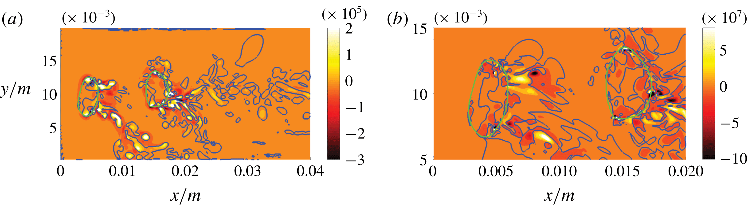
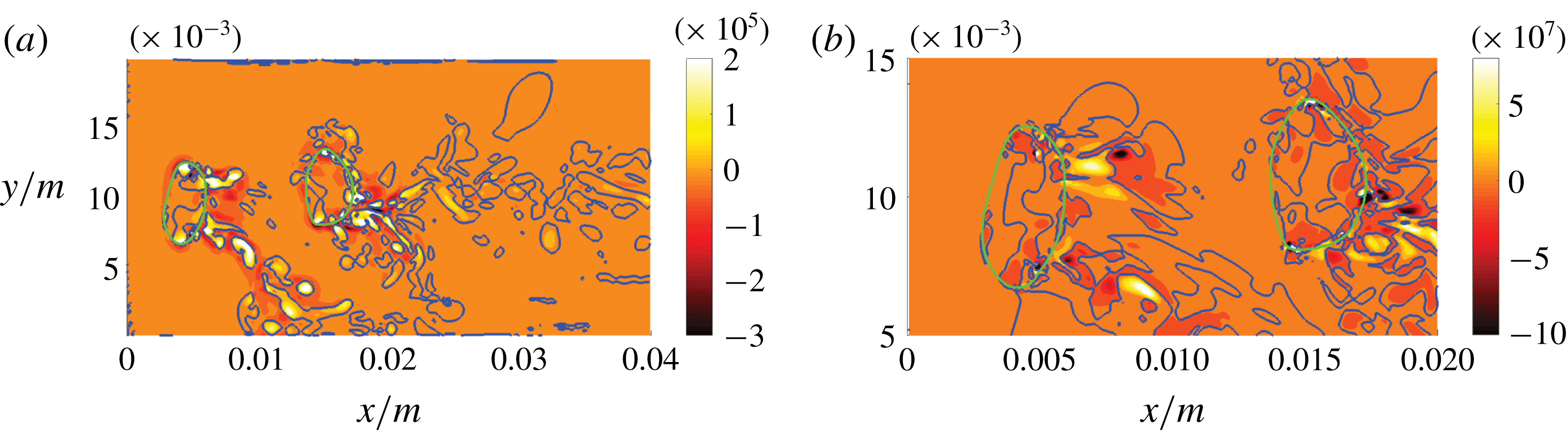
can be seen in figure 7. The laterally oriented vortex tail of the first bubble originates due to the periodic non-straight trajectory of the freely moving and deforming bubbles. Distinct peaks of
 $Q$
can be identified close to regions of high interface curvature and in the proximate bubble wakes. Particularly in the mean flow direction, there appears to be significant transport of vorticity across the interface, indicated by
 $Q>0$
. Agreeing with the diffusive and dissipative nature of turbulence, the intensity of
 $Q$
decreases generally downstream of the bubbles. The blue
 $Q=0$
isoline gives an indication whether the flow is locally strain-dominated (
 $Q<0$
) or vorticity-dominated (
 $Q>0$
). However,
 $R$
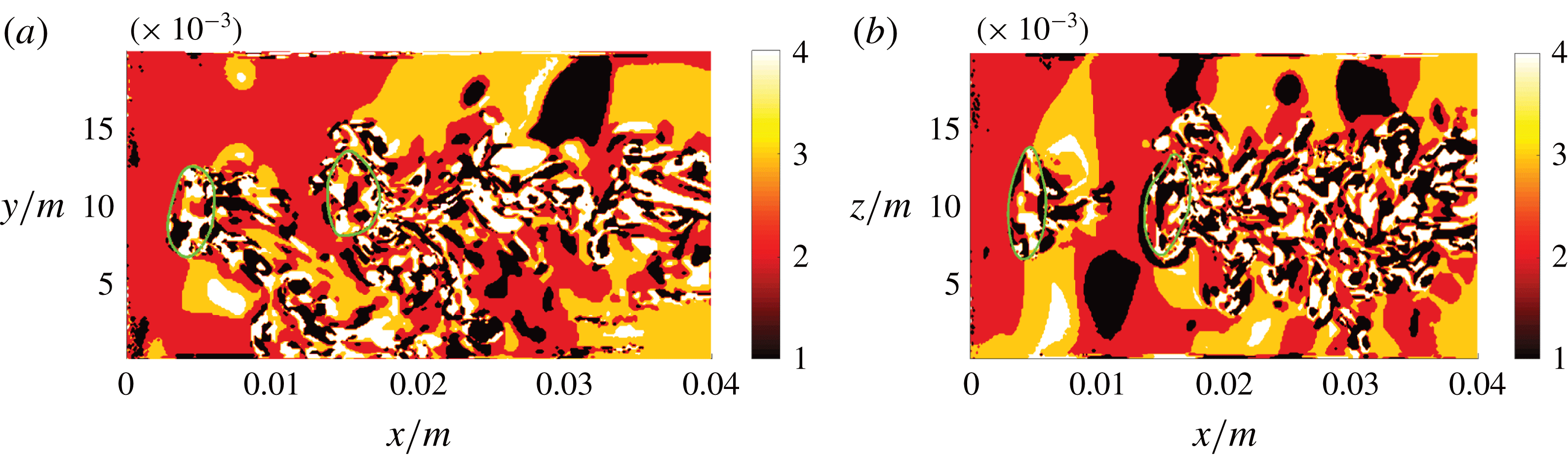
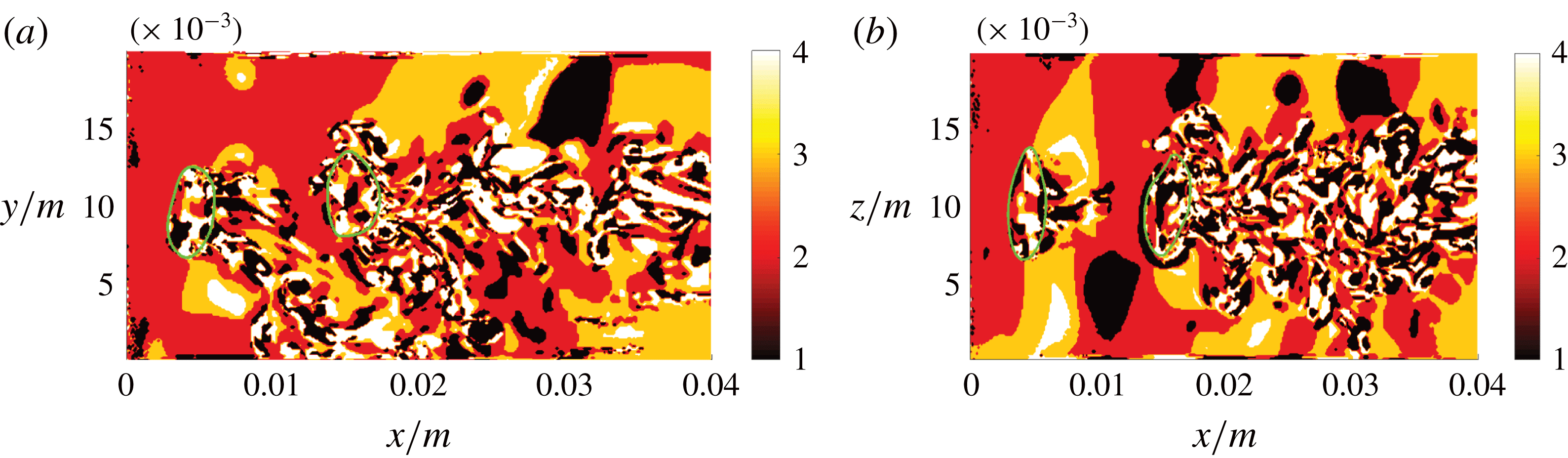
is additionally necessary for the completion of the flow topology classification as depicted in figure 8(a), since the
 $Q$
and
 $R$
fields are obviously not congruent. Besides larger regions of
 $R<0$
(vortex stretching) and
 $R>0$
(vortex compression) in the bubble wake, distinct peaks of
 $R$
are restricted to the immediate vicinity of the interface.
A second spanwise slice of the topology field (rotated by
 $90^{\circ }$
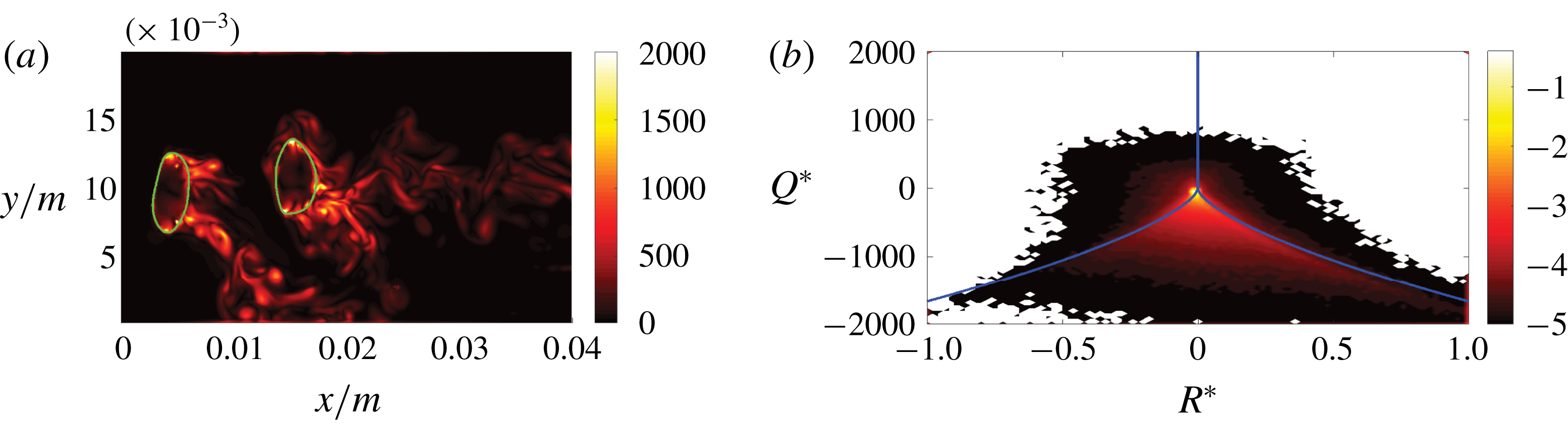
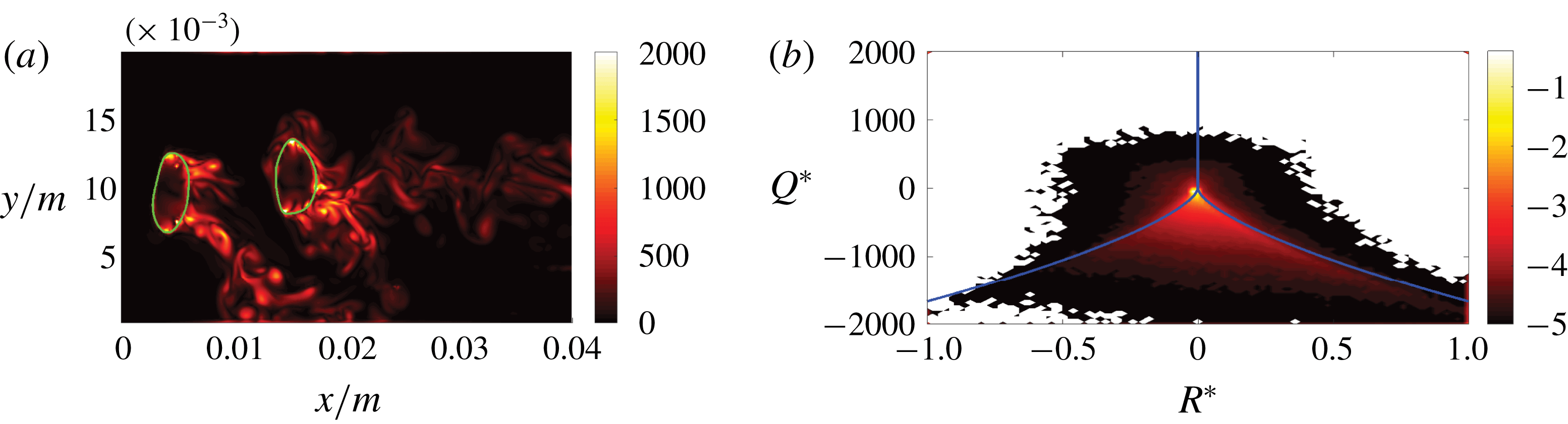
around the channel axis compared to the first slice) in figure 8(b) provides an impression as to how the flow behaviour changes in the azimuthal direction. While the behaviour in the gaseous phase is very similar in both slices, it is clearly different in the liquid phase, which is mainly a consequence of the non-straight bubble trajectory. In addition to the topology field, the vorticity field is presented in figure 9(a) to point out the strong link between the two fields, as elaborated in § 3.
DNS case A: slices of the
 $Qs^{2}$
field (a) and the magnified
 $Rs^{3}$
field (b) in the
 $x$
–
 $y$
direction. Green and blue lines indicate the phase interface and the
 $Q=0$
or
 $R=0$
isocontour, respectively.
DNS case A: slices of the flow topology field in the
 $x$
–
 $y$
direction (a) and
 $x$
–
 $z$
direction (b), where 1–4 in the colour bar refer to S1–S4, respectively. The green line indicates the phase interface.
DNS case A: slice of the
 $|\unicode[STIX]{x1D74E}|\,s$
field in the
 $x$
–
 $y$
direction (a), where the green line indicates the phase interface, and joint probability density function with common logarithmic scale of
 $Q^{\ast }=Q/\langle Q\rangle$
and
 $R^{\ast }=R/\langle R\rangle$
for the liquid phase (b); the blue lines indicate the topology borders
 $r_{1a}$
,
 $r_{1b}$
and
 $r_{2}$
.
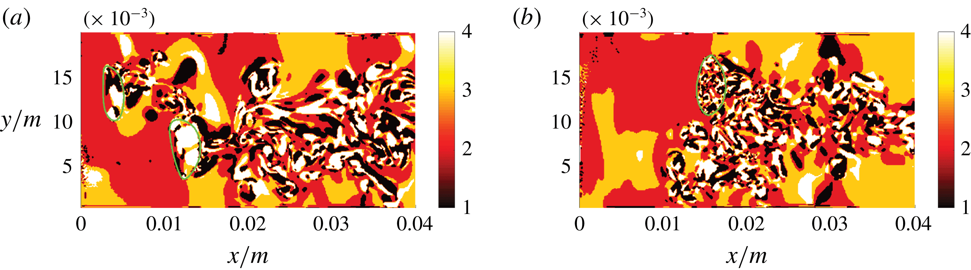
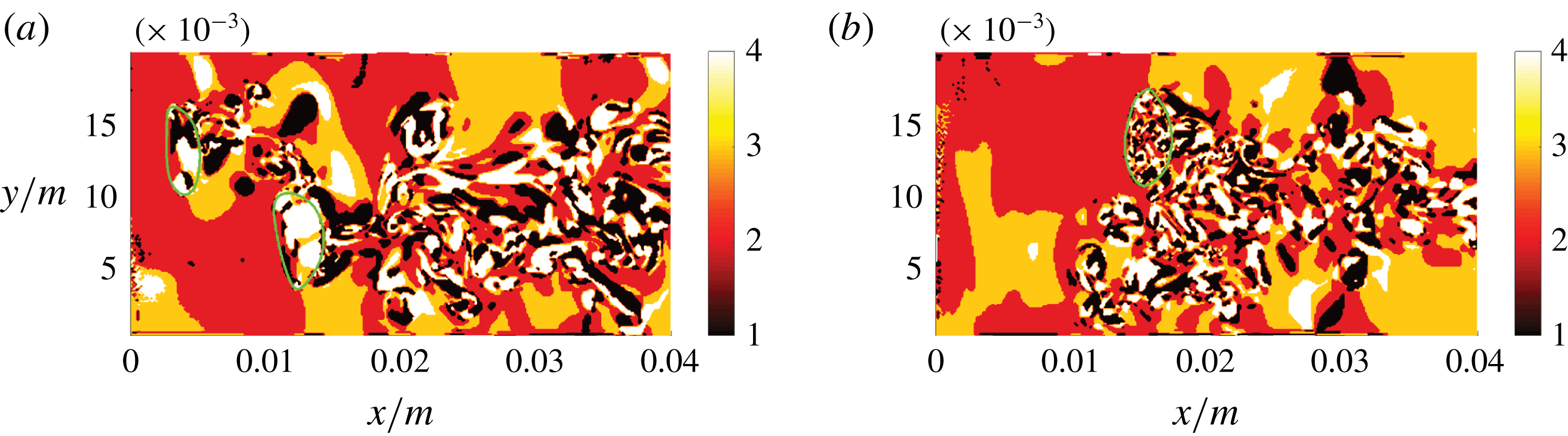
DNS case B, modified gas density (a), and DNS case C, modified gas viscosity (b): slices of the flow topology fields, where 1–4 in the colour bar refer to S1–S4, respectively.
An overall picture of the topology distribution in the liquid phase is given by the joint probability density function of
 $Q^{\ast }=Q/\langle Q\rangle$
and
 $R^{\ast }=R/\langle R\rangle$
, the mean-normalized equivalents of the second and third invariant, in figure 9(b). Owing to the large scale disparity, a logarithmic scale (base 10) is used. For the examined configuration, it can be stated that S2 and S3 are the dominant topologies in the liquid phase. Besides the dominant peak that is close to the origin, a tail to the bottom right, as for the typical teardrop shape in single-phase turbulence (Davidson Reference Davidson2015), becomes evident. However, the strong alignment with the topology borders
 $r_{1a}$
and
 $r_{1b}$
is unknown from single-phase flows, or at least less pronounced. Owing to the much smaller number of samples, the joint probability density function of the gaseous phase is less reliable and therefore not included here. It is the primary goal of the following cases to explain the higher volume fraction of focal topologies inside the air bubbles, and the major vorticity accumulation at regions of high interface curvature.
5.2 Cases B and C (modified gas properties)
The fluid properties of the gaseous phase are modified successively in order to understand the origin of the difference in flow topologies between the liquid and gaseous phases. Several non-zero terms of the vorticity transport equation (3.9) are directly dependent on the density or on the density gradients. Instead of setting equal densities, which would prevent a buoyancy-driven motion of the bubbles, the gas density is increased by two orders of magnitude (
 $\unicode[STIX]{x1D70C}_{g}=\unicode[STIX]{x1D70C}_{l}/8.318$
) in case B. In case C, identical kinematic viscosities in both phases (
 $\unicode[STIX]{x1D708}_{g}=\unicode[STIX]{x1D708}_{l}$
) are imposed. According to Davies & Taylor (Reference Davies and Taylor1950), the terminal rise velocity of large bubbles, which are similar to this study, can be approximated by
 $u_{T}=0.707\sqrt{gD_{b}}$
, i.e. it is largely independent of the density and viscosity. However, viscous damping and the Kolmogorov length scale
 $\unicode[STIX]{x1D702}=(\unicode[STIX]{x1D708}^{3}/\unicode[STIX]{x1D716})^{1/4}$
in the gaseous phase are decreased by the viscosity modification. Influences on vorticity production may come from the changed velocity field and its boundary layer at the interface, with a particular relation to terms
 $T_{2}$
and
 $T_{31}$
. Term
 $T_{32}$
also gets affected but it only diffuses and dissipates vorticity instead of generating it.
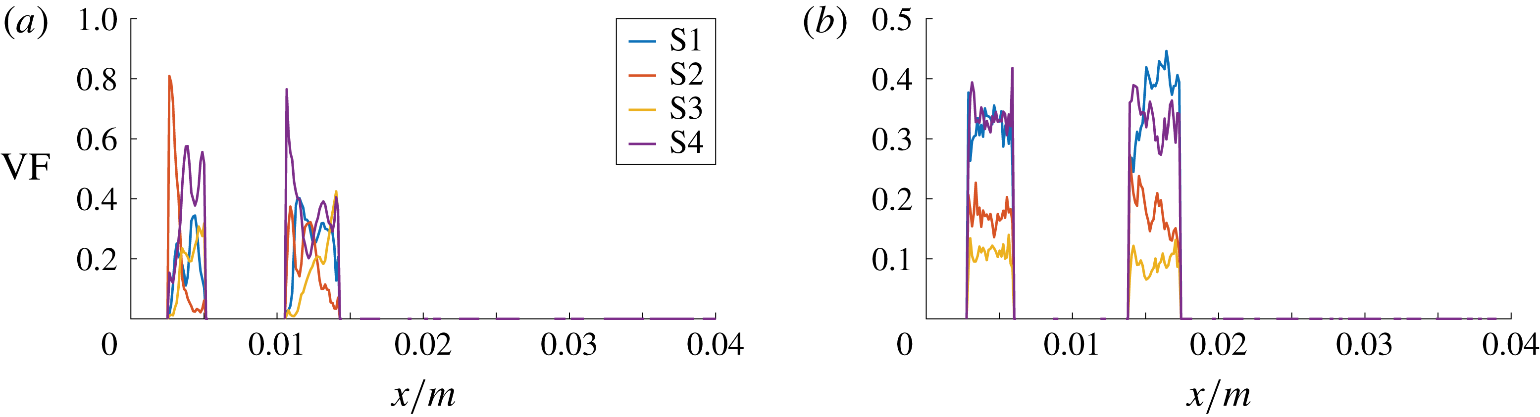
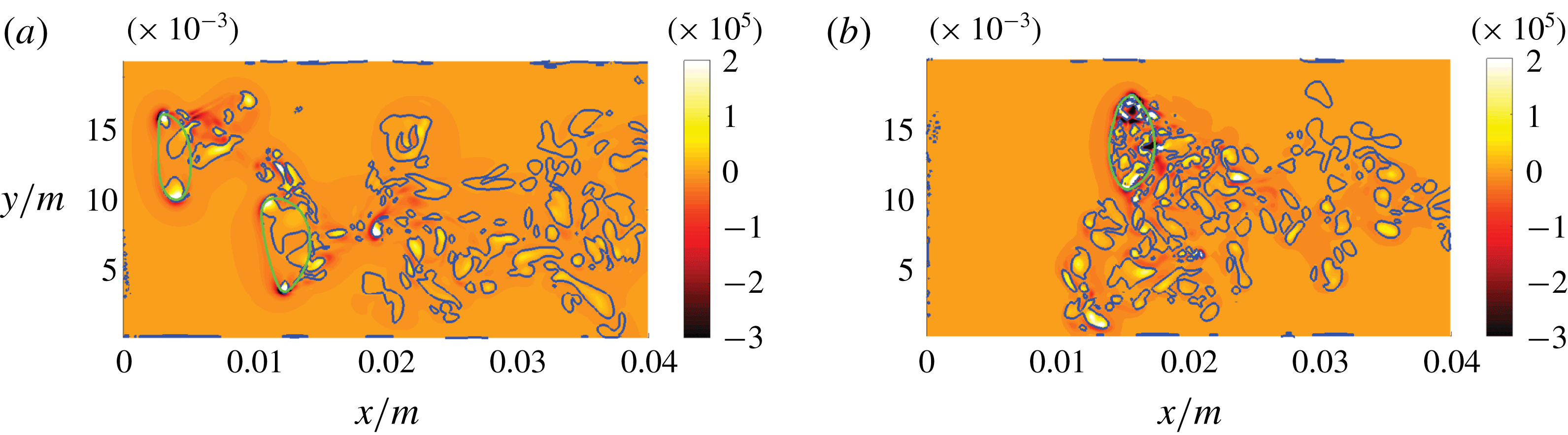
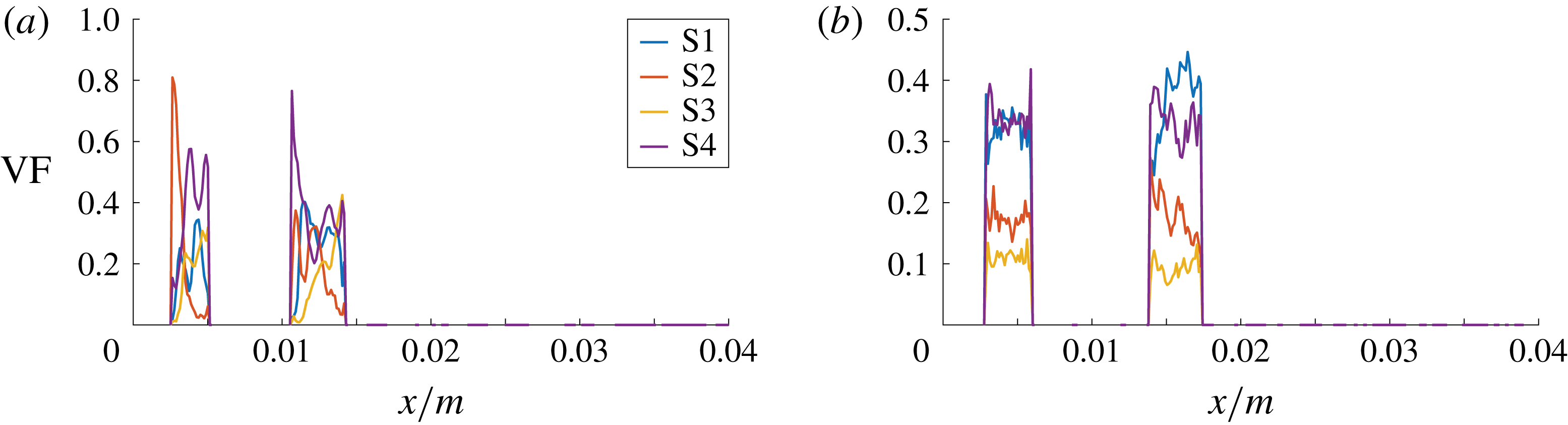
Figure 10 shows no significant changes for case B, whereas the size of topology islands in the gaseous phase is clearly affected in case C. The first bubble is not intersected by the visualized slice in case C. The decreased viscous dissipation in the bubble obviously leads to enhanced turbulent ‘mixing’, which, together with the large number of small topology islands, gives rise to a more uniform distribution of topology volume fractions (figure 11
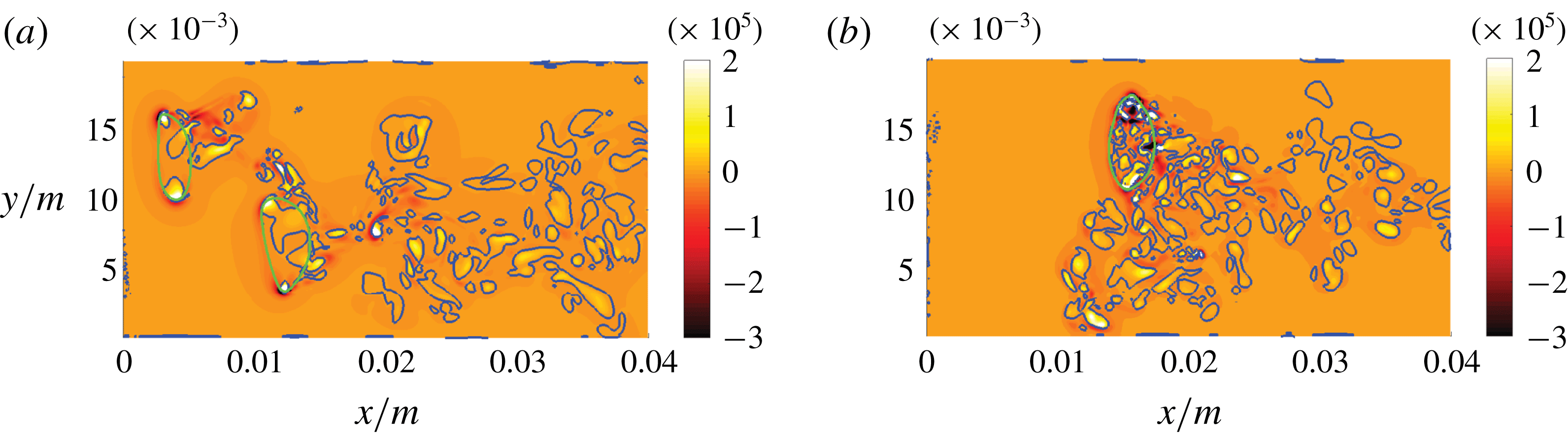
b). The dominance of focal topologies inside the bubble is maintained for both cases; cf. table 2. As is apparent from figure 12, the qualitative behaviour in terms of distinct
 $Q$
peaks at the regions of high interface curvature is unaffected as well. It can be concluded that the variation of density and viscosity, and thus the corresponding gradients at the interface, influence the situation only to a limited degree.
As discussed in § 6, Tripathi, Sahu & Govindarajan (Reference Tripathi, Sahu and Govindarajan2014) argued that vorticity would eventually accumulate in the lighter fluid independent of the viscosity ratio. However, there is numerical evidence, with some analytical support, showing that the vorticity maximum can appear in the denser fluid as well (Farsoiya, Mayya & Dasgupta Reference Farsoiya, Mayya and Dasgupta2017). Using a linearized prediction applicable only to the vorticity values immediately above and below the interface, Farsoiya et al. (Reference Farsoiya, Mayya and Dasgupta2017) found that the vorticity jump across the interface generally depends on both the density and viscosity ratio of the two fluids. Furthermore, vorticity can be produced in the bulk of both phases and, therefore, vorticity peaks can also appear in the denser fluid. Such behaviour can actually be seen in the vorticity field of the reference case (case A) in figure 9(a). The nonlinear accumulation effect due to density differences could not be entirely excluded in case B, as the density in the gaseous phase is still lower than in the liquid phase. It is however worth noting that the dominance of the focal topologies is also observed for the analytical creeping-flow solution (§ 4), where the density plays no role.
DNS case B, modified gas density (a), and DNS case C, modified gas viscosity (b): axial volume fraction distribution of flow topologies for the gaseous phase.
DNS case B, modified gas density (a), and DNS case C, modified gas viscosity (b): slices of the
 $Qs^{2}$
field. The green and blue lines indicate the phase interface and the
 $Q=0$
isocontour, respectively.
5.3 Case D (neglected surface tension, ellipsoidal bubble shape)
After inspecting the jump of fluid properties at the interface, the influences of the capillary force in terms of vorticity production can now be analysed. While
 $\unicode[STIX]{x1D70C}_{g}$
and
 $\unicode[STIX]{x1D708}_{g}$
are reset to their original values,
 $\unicode[STIX]{x1D70E}=0$
was imposed as soon as a characteristic ellipsoidal bubble shape was reached. To prevent the immediate disintegration of the bubbles, the phase interface (i.e. the
 $\unicode[STIX]{x1D6FC}$
field) was frozen at the same time, and the flow simulation was continued for at least one through-flow time. Varying
 $\unicode[STIX]{x1D70E}$
smoothly was not considered an option because of the interconnected strong impact on bubble deformability. According to (3.9), term
 $T_{53}$
can produce vorticity even in the absence of a jump of fluid properties at the interface. Case D does not solely show the effect of missing term
 $T_{53}$
, as further potential fluctuation sources are missing in this simulation: the unsteadiness of bubble deformation and the bubble trajectory.
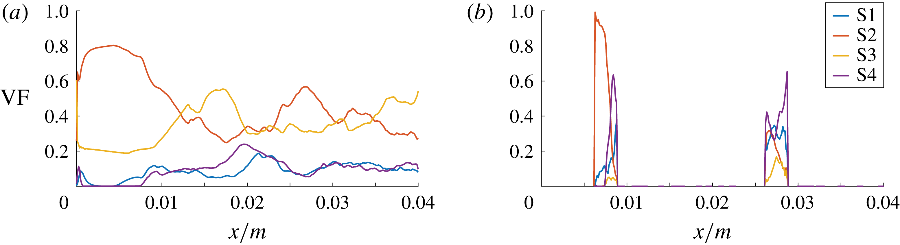
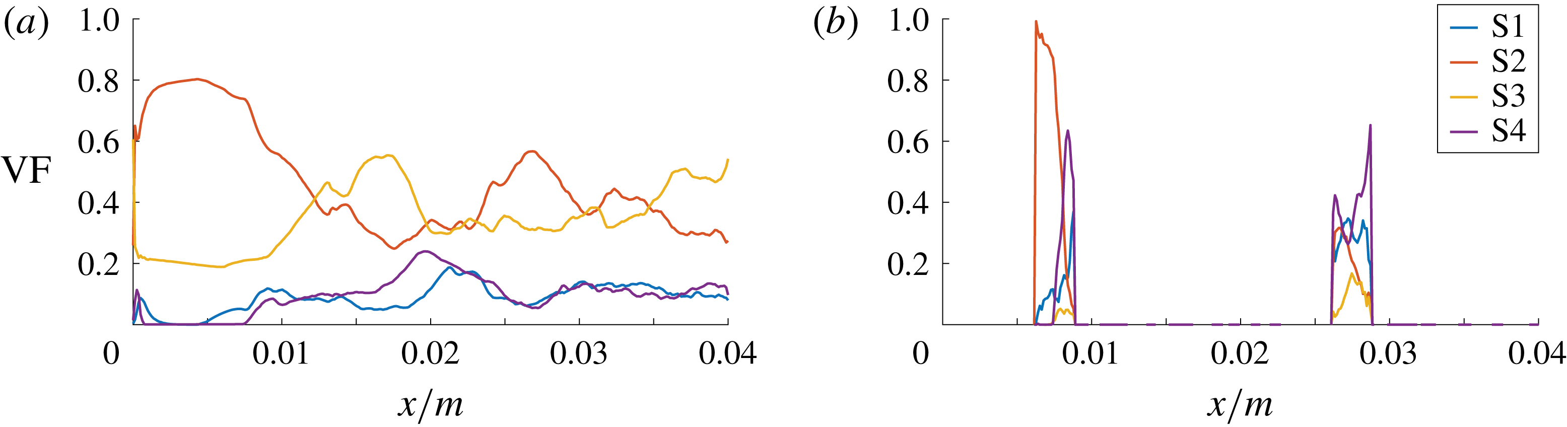
The axial volume fraction distribution in figure 13 reveals a generally lower level of focal topologies in the liquid phase, when compared to the reference case with free bubble motion and non-zero
 $\unicode[STIX]{x1D70E}$
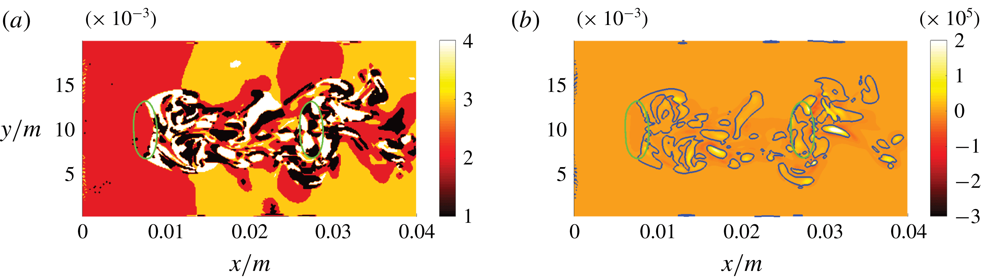
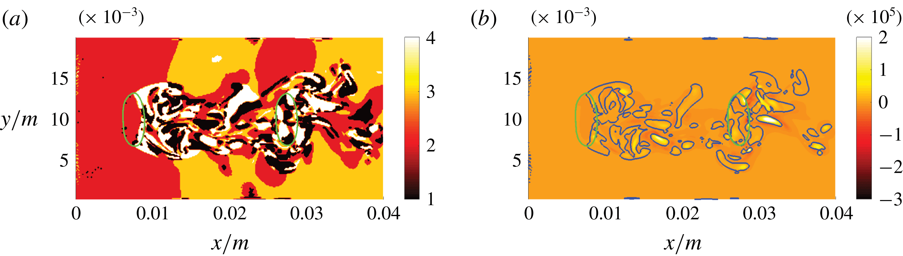
(case A). The corresponding distribution in the gaseous phase suggests a largely different behaviour of the first and second bubble, which is confirmed by figure 14. Nodal topology S2 prevails in the laminar flow facing first bubble, whereas the topology distribution in the second bubble is similar to the reference case (case A). For both bubbles, no distinct peaks of
 $Q$
can be observed in the regions of highest interface curvature. To facilitate a direct comparison with the other cases, the colour scale is identical in all
 $Q$
plots. Some mechanism of vorticity production is apparently suppressed (by exclusion of
 $T_{53}$
and modification of the flow field due to the absence of the capillary pressure jump), but turbulence is still being induced by vortex shedding in the wake of the bubbles. This behaviour at the trailing edge of the bubble might be promoted by the decrease of kinematic viscosity.
DNS case D: axial volume fraction distribution of flow topologies for the liquid phase (a) and gaseous phase (b).
DNS case D: slices of the flow topology field (a), where 1–4 in the colour bar refer to S1–S4, respectively, and corresponding
 $Qs^{2}$
field (b). The green and blue lines indicate the phase interface and the
 $Q=0$
isocontour, respectively.
5.4 Case E (neglected surface tension, spherical bubble shape)
The set-up of case E is identical to case D, with the exception of the frozen bubble shape. Instead of ellipsoidal, it is spherical, i.e. identical to the initial condition in terms of the
 $\unicode[STIX]{x1D6FC}$
field. A steady quasi-laminar solution develops, which makes it easier to interpret than the fully turbulent cases. It is especially suited to explaining the exchange of nodal topologies S2 and S3 in the liquid phase at the bubble locations, which occurs also in the turbulent cases. The obtained velocity field (not shown here) shows qualitative agreement with the analytical creeping-flow solution by Hadamard and Rybczynski (Clift et al.
Reference Clift, Grace and Weber2005; Sadhal et al.
Reference Sadhal, Ayyaswamy and Chung2012), which strictly holds only for inertialess spherical bubbles at a very low Reynolds number; cf. § 4. The solution is surely different from the flow around rigid spheres, for which an unsteady von Kármán vortex street develops in the wake (Sakamoto & Haniu Reference Sakamoto and Haniu1990). Owing to the absence of the capillary pressure jump (
 $\unicode[STIX]{x1D70E}=0$
), the obstacle effect of the bubbles is reduced to some degree. However, as argued in § 3, the capillary pressure jump itself does not generate any vorticity. Term
 $T_{53}$
of the vorticity transport equation (3.9) is irrelevant to this case since it is identically zero for perfectly spherical bubbles, even for
 $\unicode[STIX]{x1D70E}>0$
.
The axial evolution of the topology volume fractions in the liquid phase and a slice of the flow topology field are depicted in figure 15. A regular oscillating pattern of nodal topologies S2 and S3 evolves in the liquid phase while the (spurious) focal topologies S1 and S4 remain at a very low level. It can be understood that flow topologies S2 (unstable node) and S3 (stable node) correspond to the streamline divergence ahead of the bubble centre and streamline convergence behind the bubble centre, respectively. Similar to the steady semi-analytical solution discussed in § 4, a nodal-to-focal-to-nodal topology transition seems to occur in the gaseous phase. The first and second bubble do not show any differences in that regard.
DNS case E: axial volume fraction distribution of flow topologies for the liquid phase (a) and corresponding slice of the topology field (b), where 1–4 in the colour bar refer to S1–S4, respectively.
6 Closing remarks
The purpose of this study is to shed some light on the mechanism of turbulence production in bubbly two-phase flows. Several physical insights have been obtained on the basis of a local flow topology analysis. Whereas the volume fraction of nodal or focal topologies in the liquid phase is largely a consequence of the specific simulation set-up, the dominance of the focal topologies in the gaseous phase is expected to appear consistently. As such, in order to find the main reason for this behaviour, the mathematical model has been successively manipulated with respect to the fluid properties of the gaseous phase (i.e. by employing the process of elimination). Increasing the gas density by two orders of magnitude (case B), as well as imposing equal kinematic viscosities in both phases (case C), influences the topology budgets only to a limited degree. If the capillary force is artificially set to zero while freezing the bubble shape (ellipsoidal bubble in case D, spherical bubble in case E), the vorticity level is generally lower in both phases when compared to the physical reference case (case A). However, both phases still contain focal topologies, even for the steady quasi-laminar flow in case E (spherical bubble shape).
As long as the flow is stable, as in the steady analytical solution discussed in § 4, the dynamic viscosity ratio would determine whether the vorticity maximum in the bubble vicinity is located in the liquid or gaseous phase. According to Tripathi et al. (Reference Tripathi, Sahu and Govindarajan2014), it follows from stability arguments (Dixit & Govindarajan Reference Dixit and Govindarajan2010) that vorticity tends to accumulate in the lighter fluid independent of the viscosity ratio and the concaveness/convexness of the interface. It can be speculated that this nonlinear accumulation effect is particularly important when the bubble-affected flow becomes unstable, like in the unsteady and turbulent cases A, B, C and D. The vorticity and topology distributions are obviously strongly linked, as elaborated in § 3.
7 Conclusions and outlook
The dominance of focal topologies in the gaseous phase of bubbly flows seems to be connected to strong vorticity budgets at the regions of simultaneous high fluid velocity and high interface curvature. This general behaviour is already evident from the analysis of the analytical creeping-flow solution for very low Reynolds numbers. In the same vein, additional nonlinear effects in unsteady turbulent flows are responsible for the tendency of vorticity accumulation in the lighter fluid. Nevertheless, there is a strong commonality between laminar and turbulent flows regarding the dominant topologies: nodal topology S2 ahead of the bubble due to streamline divergence, focal topologies S4 and S1 within the bubble, and nodal topology S3 in the wake of the bubble due to streamline convergence. Furthermore, it is observed that the vorticity is also transported across the interface in the turbulent cases.
Imposing certain bubble shapes and setting the capillary force to zero significantly changes the vorticity and topology distribution in both phases. More than one influencing factor is affected by this modification. On the one hand, the flow field especially within the bubble is altered due to the absence of the capillary pressure jump. On the other hand, a specific term of the vorticity transport equation related to surface tension and gradients of interface curvature, responsible for the induction of vortical motion directly at the interface, is excluded. Besides the known mechanisms (unsteadiness of bubble deformation, the bubble trajectory and vortex shedding in the bubble wake), the latter term represents another potential source of turbulence production that lends itself to further investigation.
It is likely that a combination of different effects has to be considered to fully explain the generation of turbulence by bubbles – a thorough quantification is required. Since the additional mechanism for vorticity production is absent in single-phase flows, state-of-the-art modelling strategies should be reassessed in that regard. For example, in the LES context, the interface micro-curvature remains unresolved and corresponding subgrid modelling might be necessary.
Acknowledgements
Support by the German Research Foundation (Deutsche Forschungsgemeinschaft – DFG, GS: KL1456/4-1) is gratefully acknowledged. The authors also express their gratitude to the developers of PARIS for providing the source code.