2 Experimental method

As indicated in figure 1, five different kinds of interfaces, including a single-mode (SM), a circular-arc (CA), a trapezoid (TR), a square-waveform (SW) and a saw-tooth (ST) interface, are involved. For each case, the wavelength ( $\unicode[STIX]{x1D706}$ ) is 60 mm and two initial amplitudes, one satisfying the small-perturbation hypothesis and the other not, are considered, respectively. The Fourier expansions of the quasi-single-mode interfaces with small initial amplitude are presented as follows:

(2.1) $$\begin{eqnarray}\displaystyle \left.\begin{array}{@{}l@{}}y_{CA}=a_{i0}[-1.042\cos (kx)+0.051\cos (3kx)-0.011\cos (5kx)+\cdots \,],\\ y_{TR}=a_{i0}[-1.163\cos (kx)+0.159\cos (3kx)+0.034\cos (5kx)-\cdots \,],\\ y_{SW}=a_{i0}[-1.273\cos (kx)+0.424\cos (3kx)-0.255\cos (5kx)+\cdots \,],\\ y_{ST}=a_{i0}[-0.811\cos (kx)-0.090\cos (3kx)-0.032\cos (5kx)-\cdots \,],\end{array}\right\} & & \displaystyle\end{eqnarray}$$

where $y_{CA}$ , $y_{TR}$ , $y_{SW}$ and $y_{ST}$ represent the Fourier expansions of the circular-arc, trapezoid, square-waveform and saw-tooth interfaces, respectively. The Fourier expansions of the quasi-single-mode interfaces with high initial amplitude are the same as those of interfaces with small initial amplitudes except the circular-arc one. In this work, the Fourier expansion of the circular-arc interface with high initial amplitude is $y_{CA}=a_{i0}[-1.134\cos (kx)+0.188\cos (3kx)-0.084\cos (5kx)+\cdots \,]$ . One can observe that the fundamental mode for all the four quasi-single-mode interfaces is the most significant one among all the modes, which means the fundamental mode will dominate the interface evolution. For the square-waveform interface, although the third mode has an amplitude which is nearly 33 % of its fundamental mode, the amplitude ratio of the superposition of the fundamental mode with the third mode over the fundamental mode is 94 %. As a result, the fundamental mode still dominates. It can be found that some of the high-order modes in circular-arc, trapezoid and square-waveform interfaces are opposite to the fundamental mode in sign, and the deviation degree of these three interfaces from the single-mode one increases successively. For the saw-tooth interface, differently, the signs of the high-order modes are the same as the fundamental one.

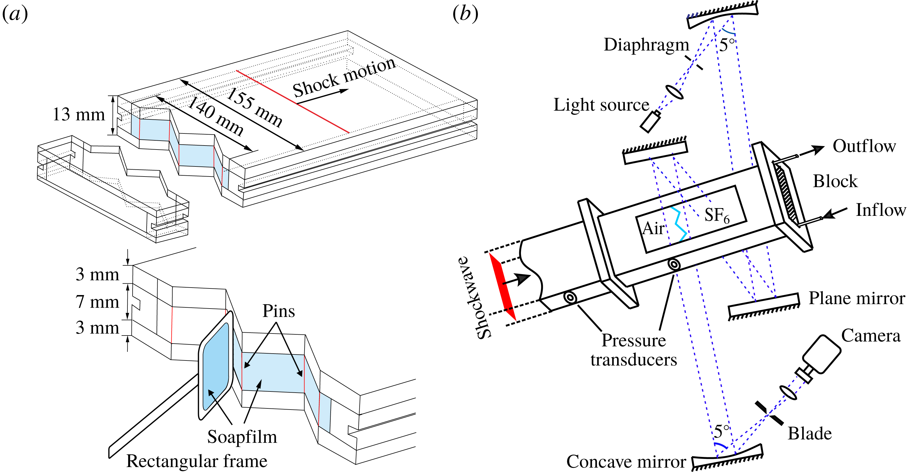
To create the initial interface, taking the saw-tooth interface as an example as shown in figure 2(a), two transparent devices with a width of 140 mm are first manufactured using acrylic plates with a thickness of 3 mm. For the single-mode and circular-arc interfaces, the adjacent boundaries are carefully engraved to be of a single-mode or circular-arc shape with a depth of 0.2 mm. To restrict the soap film to the designed shape, two thin filaments with a thickness of 0.5 mm are normally attached to the inner surfaces of the upper and lower plates, respectively. Thus the filament protrusion is only 0.3 mm, having a negligible influence on the flow. The shape of the circular-arc interface is created by pieces of symmetrical arcs, and the curvature radius of each point on the interface is the same (30.125 mm and 15 mm for small and high initial amplitudes, respectively). For the other three interfaces, to avoid the pressure singularity caused by surface tension at the vertex (Wang, Si & Luo Reference Wang, Si and Luo2013), thin pins with a diameter of 0.148 mm are arranged at the vertex to restrict the soap films. For each vertex, the number of pins is dependent on the vertex angle. For the saw-tooth and trapezoid interfaces with small initial amplitude, only one pin is used. For the trapezoid interface with high initial amplitude and the two square-waveform interfaces, two pins are used at each vertex. For the saw-tooth interface with high initial amplitude, three pins are used. The effects of pins at the vertex on the shock wave movement, interface morphology and the vorticity deposition have been investigated in previous work (Wang et al. Reference Wang, Si and Luo2013; Zhai et al. Reference Zhai, Wang, Si and Luo2014) by experiments and numerical simulations. The results have proved that the pins have little influence on the interface morphology and vorticity deposition. Note that in previous work (Sadot et al. Reference Sadot, Erez, Alon, Oron, Levin, Erez, Ben-Dor and Shvarts1998; Jourdan & Houas Reference Jourdan and Houas2005; Vandenboomgaerde et al. Reference Vandenboomgaerde, Rouzier, Souffland, Biamino, Jourdan, Houas and Mariani2018) a wire mesh was generally used to hold an interface. The pins have similar drawbacks to the wire mesh. For example, the pins will enhance the mixing near the vertex, supporting a modest increase in amplitude growth rate (Prasad et al. Reference Prasad, Rasheed, Kumar and Sturtevant2000), and also will introduce short-wavelength perturbations to the initial interface (Vandenboomgaerde et al. Reference Vandenboomgaerde, Rouzier, Souffland, Biamino, Jourdan, Houas and Mariani2018). However, compared with the wire mesh which will block the flow significantly, the pins have limited effects on the flow because they are only placed at each vertex. Although the pins may influence the high-order modes, they have negligible effect on the fundamental mode (Vandenboomgaerde et al. Reference Vandenboomgaerde, Rouzier, Souffland, Biamino, Jourdan, Houas and Mariani2018). As a result, the effects of the pins in the present work are ignored since the fundamental mode is dominant.

Figure 2.

Schematics of the creation of a saw-tooth interface (a) and the schlieren photography adopted in the experiment (b).

Prior to the interface formation, the filaments or the edges of the acrylic plates are properly wetted by soap solutions (made of 78 % distilled water, 2 % sodium oleate and 20 % glycerine in mass). Then, a rectangular frame, the edges of which have been dipped into an appropriate amount of soap solutions, is pulled along the filaments or the edge of the acrylic plates. A soap film interface with the designed shape is then generated on the surface. Subsequently, the auxiliary framework is gently inserted until it is completely connected to the corresponding device. After that, the framework with soap film on its surface is slowly inserted into the test section. To form an air/ $\text{SF}_{6}$ interface, air at the right-hand side of the interface must be replaced by $\text{SF}_{6}$ prior to the experiment. For this purpose, $\text{SF}_{6}$ is injected into the test section through an ‘Inflow’ hole, and air is gradually exhausted through an ‘Outflow’ hole, as shown in figure 2(b). 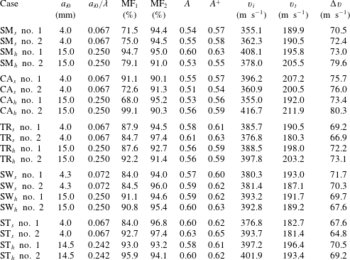A gas concentration detector is placed at the ‘Outflow’ hole to monitor the purity of $\text{SF}_{6}$ at the right-hand side of the interface. In the experiment, when the volume fraction of the oxygen measured by the detector is lower than 0.5 %, the gas inflation is stopped. Then the experiment is conducted as soon as possible to reduce the gas diffusion. In fact, during the gas inflation process, the gas exchange through the interface has already begun, and the gas inflation time influences the purity of gases. Moreover, after the gas inflation ends and before the experiments starts, the time interval also allows gas diffusion. These time intervals are difficult to keep exactly the same for different experimental runs. As a result, the gas components at both sides of the interface will vary a little from run to run, and the shock velocity will change when it enters the test section although the shock tube facility has a good repeatability. The gas components at both sides are determined by the shock velocities and one-dimensional (1-D) gas dynamics theory as given in table 1, in which $A=(\unicode[STIX]{x1D70C}_{2}-\unicode[STIX]{x1D70C}_{1})/(\unicode[STIX]{x1D70C}_{2}+\unicode[STIX]{x1D70C}_{1})$ is Atwood number with $\unicode[STIX]{x1D70C}_{2}$ and $\unicode[STIX]{x1D70C}_{1}$ being the densities of gases at the right- and left-hand sides of the interface, respectively. In our work, more than one successful experimental run was performed for each case. In table 1, the subscript $s$ and $h$ correspond to the interfaces with small and high initial amplitudes, respectively. The numbers 1 and 2 represent the typical experimental runs, respectively.

Table 1.

Experimental initial parameters for all cases: $a_{i0}$ is the initial amplitude of the interface; $\text{MF}_{1}$ ( $\text{MF}_{2}$ ) is the mass fraction of air ( $\text{SF}_{6}$ ) at the left (right) side of the interface; $A=(\unicode[STIX]{x1D70C}_{2}-\unicode[STIX]{x1D70C}_{1})/(\unicode[STIX]{x1D70C}_{2}+\unicode[STIX]{x1D70C}_{1})$ is pre-shock Atwood number with $\unicode[STIX]{x1D70C}_{2}$ and $\unicode[STIX]{x1D70C}_{1}$ being the densities of gases at the right and left sides of the interface, respectively; $A^{+}$ is post-shock Atwood number; $v_{i}$ is the velocity of the incident shock; $v_{t}$ is the velocity of the transmitted shock; $\unicode[STIX]{x0394}v$ is the velocity of post-shock flow. The subscripts $s$ and $h$ correspond to the interfaces with small and high initial amplitudes, respectively. The numbers no. 1 and no. 2 represent the typical experimental runs, respectively.

Experiments are conducted in the same shock tube as previous work (Liu et al. Reference Liu, Liang, Ding, Liu and Luo2018). The cross-sectional area of the test section is 140 mm $\times$ 13 mm. As a result, the interface height is 7.0 mm because there is an acrylic plate with a thickness of 3 mm at each side in the test section. Note that the actual height of the single-mode and circular-arc interfaces is 6.4 mm because these two interfaces are restricted by the filaments with a 0.3 mm protrusion inside the flow field. The incident shock Mach number measured by piezoelectric transducers mounted in the driven section is 1.20 $\pm$ 0.03 from all the measurements, which indicates that the shock tube facility has a very good repeatability. Illuminated by a continuous light source (CEL-HXF300, maximum power output 249 W), the shocked flow is captured by high-speed schlieren photography as shown in figure 2(b). The frame rate of the camera (FASTCAM SA5, Photron Limited) is 50 000 f.p.s., and the exposure time is $0.37~\unicode[STIX]{x03BC}\text{s}$ . The spatial resolution of the schlieren image is $0.28~\text{mm}~\text{pixel}^{-1}$ . The ambient pressure and temperature are 101.3 kPa and 293 K, respectively.

The three-dimensional (3-D) effect of a single-mode interface formed by the soap film technique has been discussed in our previous work (Luo, Wang & Si Reference Luo, Wang and Si2013). Because the gases on both sides of the interface are at ambient pressure, the soap film interface formed has a zero mean curvature and the geometry can be characterized as minimum surface (Isenberg Reference Isenberg1992). In this work, for the two cases with small and high initial amplitudes, the wavelength $\unicode[STIX]{x1D706}$ is fixed at 60 mm, the amplitudes of the boundary slice are 4 and 15 mm, respectively. When the interface height is 20 mm, the amplitudes of the symmetry slices for the two cases are 2.48 and 8.42 mm, respectively. The amplitude ratios of the symmetry slice over the boundary slice are 62 % and 56 %, respectively, indicating a significant 3-D effect. When the interface height reduces to 7.0 mm, the amplitudes of the symmetry slices for the two cases are 3.75 and 14.00 mm, respectively. The amplitude ratios of the symmetry slice over the boundary slice are 93.75 % and 93.33 %, respectively. As a result, it is believed that the reduction of the interface height can reduce the 3-D effect, and the 3-D effect in this work is insignificant.

After the incident shock with Mach number of 1.2 impacts the interface, the flow behind the transmitted shock can be regarded as laminar and incompressible. As a result, the displacement thickness of the boundary layer ( $\unicode[STIX]{x1D6FF}^{\ast }$ ) can be approximately calculated by the following expression:

(2.2) $$\begin{eqnarray}\displaystyle \unicode[STIX]{x1D6FF}^{\ast }=1.72\sqrt{\frac{\unicode[STIX]{x1D707}x}{\unicode[STIX]{x1D70C}\unicode[STIX]{x0394}v}}, & & \displaystyle\end{eqnarray}$$

where $x$ ( $=100$  mm measured from experiment) is the maximum distance that the interface moves when image recording ends. For simplification, the parameters of pure air as ambient gas and pure $\text{SF}_{6}$ as test gas at a temperature of 293 K are adopted for estimation. Thus, $\unicode[STIX]{x1D707}=1.83\times 10^{-5}~\text{Pa}~\text{s}$ ( $\,=\,1.60\times 10^{-5}~\text{Pa}~\text{s}$ ) is the viscosity coefficient of pure air ( $\text{SF}_{6}$ ) and $\unicode[STIX]{x1D70C}=1.204~\text{kg}~\text{m}^{-3}$ ( $\,=\,6.143~\text{kg}~\text{m}^{-3}$ ) is the density of pure air ( $\text{SF}_{6}$ ); $\unicode[STIX]{x0394}v$ ( ${\sim}70.0~\text{m}~\text{s}^{-1}$ ) is the post-shock flow velocity calculated from 1-D gas dynamics. According to (2.2), the displacement thickness of the boundary layer is calculated to be about 0.24 mm for ambient gas and 0.1 mm for test gas, which is much smaller than the inner height of the acrylic plates (7.0 mm). Therefore, the effect of the boundary layer on the interface evolution is negligible.

Figure 3.

Schlieren pictures of a planar shock accelerating a planar air/ $\text{SF}_{6}$ interface. TS, transmitted shock; SI, shocked interface. Incident shock with Mach number of 1.17 passes from left to right. The unit of the numbers is ms.

On the other hand, the motion and morphology of a planar interface after a planar shock impact can be used to evaluate the boundary layer effect. Figure 3 shows the typical evolution of a planar interface impacted by a planar shock performed in this shock tube. After shock impact, the transmitted shock TS and the shocked interface SI move uniformly. Table 2 shows the comparison of experimental results with their theoretical counterparts in the 1-D shock–interface interaction for four different runs. Both the velocities of the TS and the SI agree well between the experiments and the predictions, which means that the interface motion is not influenced significantly by the boundary layer effect, because the boundary layer will accelerate the interface motion (Morgan et al. Reference Morgan, Aure, Stockero, Greenough, Cabot, Likhachev and Jacobs2012). Moreover, the growth of the planar interface thickness is mainly ascribed to the boundary layer effect (Brouillette & Sturevant Reference Brouillette and Sturevant1993; Vetter & Sturtevant Reference Vetter and Sturtevant1995). Therefore, the growth rate of the planar interface thickness can reflect the boundary layer effect. The larger the growth rate, the more significant the boundary layer effect (Brouillette & Sturevant Reference Brouillette and Sturevant1993; Vetter & Sturtevant Reference Vetter and Sturtevant1995). The growth rate of the planar interface thickness in case $I^{a}$ in Vetter & Sturtevant (Reference Vetter and Sturtevant1995) was $0.94~\text{m}~\text{s}^{-1}$ , and the authors concluded that the effects of shock-wave/boundary-layer interaction have been reduced significantly. In our shock tube, the initial conditions in Case 1 are similar to previous work, and the growth rate of the planar interface thickness is calculated as $0.84~\text{m}~\text{s}^{-1}$ , which is even smaller than that in previous work. Therefore, it is believed that the boundary layer effect in this work is not significant.

Table 2.

Comparison of experimental and theoretical parameters in the 1-D shock–interface interaction. $Ma$ , incident shock Mach number, $v_{exp}^{t}$ and $v_{the}^{t}$ respectively represent the experimental and theoretical transmitted shock velocities, $v_{exp}^{si}$ and $v_{the}^{si}$ respectively represent the experimental and theoretical shocked interface velocities.

3 Interfacial morphology and wave pattern

The experimental schlieren images for the five air/ $\text{SF}_{6}$ interfaces with small and high initial amplitudes interacting with a planar shock are presented in figures 4 and 5, respectively. To improve the spatial and temporal resolutions, the images are presented with only one wavelength because the interface is periodic and one wavelength can represent the ensemble. For all cases, the moment when the shock contacts the interface centre is defined as the initial time ( $t=0$ ). From the interface morphologies, no obvious 3-D features are observed in the flow, which also indicates that 3-D effects can be ignored.

Figure 4.

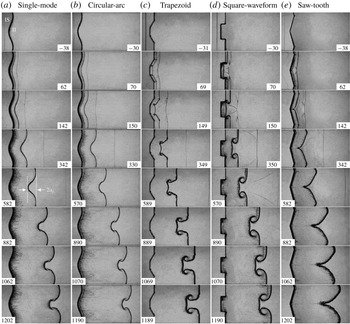
Schlieren pictures of interfaces with small initial amplitude accelerated by a planar shock wave: single-mode (a), circular-arc (b), trapezoid (c), square-waveform (d) and saw-tooth (e). Here, $a_{i}$ , interface amplitude; IS, incident shock; II, initial interface. Numbers denote the time in $\unicode[STIX]{x03BC}\text{s}$ .

For the single-mode interface with small initial amplitude as shown in figure 4(a), the incident shock bifurcates into a downstream-moving transmitted shock and an upstream-moving reflected shock after it passes through the initial interface. The interface deforms gradually because of the pressure perturbations and the baroclinic vorticity induction. At the early stage, the spike (the heavier fluid penetrating into the lighter fluid) and the bubble (the lighter fluid penetrating into the heavier fluid) grow symmetrically ( $342~\unicode[STIX]{x03BC}\text{s}$ ), indicating a linear growth of the amplitude. As the interface evolves, the high-order harmonics are generated and become significant, destroying the symmetry of the interface evolution ( $582~\unicode[STIX]{x03BC}\text{s}$ ). Later, the spike starts to roll up and a pair of small vortices appears on its shoulder ( $1062~\unicode[STIX]{x03BC}\text{s}$ ). Note that the interface morphology captured in the present study is more accurate than previous membrane results (Mariani et al. Reference Mariani, Vandenboomgaerde, Jourdan, Souffland and Houas2008). The spike head in this work is flat, which is consistent with the observation in membrane experiments (Mariani et al. Reference Mariani, Vandenboomgaerde, Jourdan, Souffland and Houas2008; Vandenboomgaerde et al. Reference Vandenboomgaerde, Souffland, Mariani, Biamino, Jourdan and Houas2014), but is different from the previous membraneless experiments (Jones & Jacobs Reference Jones and Jacobs1997; Collins & Jacobs Reference Collins and Jacobs2002; Jacobs & Krivets Reference Jacobs and Krivets2005) in which the spike head is ‘mushroom-like’. As Vandenboomgaerde et al. (Reference Vandenboomgaerde, Souffland, Mariani, Biamino, Jourdan and Houas2014) stated, the RM typical ‘mushroom-like’ structures on the interface are only made possible due to a diffusion layer at the initial interface. As illustrated in figure 4(b), both interface deformation and wave patterns in the circular-arc interface are similar to those in the single-mode case. Differently, the vortices are generated earlier in the circular-arc interface ( ${\sim}570~\unicode[STIX]{x03BC}\text{s}$ ) relative to the single-mode counterpart ( ${\sim}882~\unicode[STIX]{x03BC}\text{s}$ ) because the incident angle $\unicode[STIX]{x1D703}$ (the angle of the shock front with the interface) on the circular-arc interface surface ( $29.86^{\circ }$ ) is greater than that on the single-mode interface surface ( $22.73^{\circ }$ ), and the amplitude of vorticity deposited is proportional to $\sin \unicode[STIX]{x1D703}$ . Also, the spike head in the circular-arc case is approximately ‘mushroom-like’ due to its larger initial interface curvature.

Figure 4(c) shows the evolution of the shocked trapezoid interface. Two pairs of Mach reflections occur on the transmitted shock, resulting in the formation of two Mach stems and four triple points ( $69~\unicode[STIX]{x03BC}\text{s}$ ). The disturbed transmitted shock consists of two Mach stems and a flat part, and quickly recovers to a planar one ( $349~\unicode[STIX]{x03BC}\text{s}$ ). The vortices are quickly produced from the vertex ( $69~\unicode[STIX]{x03BC}\text{s}$ ), and are more obvious due to the larger incident angle ( $30^{\circ }$ ). A crater is observed on the spike head between a pair of vortices due to the velocity difference between the vortices and the flat part. The depth of the crater first increases (before $589~\unicode[STIX]{x03BC}\text{s}$ ), and then reduces until it disappears. An opposite direction crater with a smaller curvature is observed on the bubble head ( $149{-}589~\unicode[STIX]{x03BC}\text{s}$ ), and this crater also disappears gradually. Similarly to the trapezoid interface, Mach reflection occurs and a pair of Mach stems is formed ( $70~\unicode[STIX]{x03BC}\text{s}$ ) in the square-waveform case as presented in figure 4(d). The bubble structure is quite flat relative to other interfaces. Because the incident angle is $90^{\circ }$ for the square-waveform interface, the vortices produced the vertexes are more obvious.

The evolution of a shocked saw-tooth interface is shown in figure 4(e). Different from the work of Luo et al. (Reference Luo, Dong, Si and Zhai2016), the saw-tooth interface is periodic in this work, and the effect of flat parts on both sides of the perturbed interface on the evolution is eliminated (Luo et al. Reference Luo, Liang, Si and Zhai2019). As the incident shock moves along two straight interfaces, Mach reflection occurs quickly on the transmitted shock, and the triple point and Mach stem are clearly observed at $t=62~\unicode[STIX]{x03BC}\text{s}$ . As the interface develops, the bubble becomes ‘arc-like’ while the spike becomes sharper ( $582{-}1202~\unicode[STIX]{x03BC}\text{s}$ ). The vortices appear at very late time, which is partially ascribed to the very small incident angle ( $15^{\circ }$ ) in this case. Also, the pins used to form the vertex of the saw-tooth interface enhance the mixing near the spike head, covering the appearance of vortices (Prasad et al. Reference Prasad, Rasheed, Kumar and Sturtevant2000).

Figure 5.

Schlieren pictures of interfaces with high initial amplitude accelerated by a planar shock wave: single-mode (a), circular-arc (b), trapezoid (c), square-waveform (d), and saw-tooth (e).

Figure 5 presents the evolutions of the five kinds of interfaces with high initial amplitude. For the single-mode case as presented in figure 5(a), after the incident shock collides with the perturbed interface, Mach stems and triple points are formed on the transmitted shock ( $62~\unicode[STIX]{x03BC}\text{s}$ ). The wave patterns are more complicated compared with the case with small initial amplitude, and the secondary compressible effect becomes more significant for the high initial amplitude (McFarland et al. Reference McFarland, Greenough and Ranjan2013). As the initial amplitude increases while the wavelength remains the same, the curvature radius of the spike head decreases. The shape of the spike head gradually converts from circular-arc to flat ( $587~\unicode[STIX]{x03BC}\text{s}$ ) and a cavity even occurs at the spike centre ( $887~\unicode[STIX]{x03BC}\text{s}$ ). The scale of the cavity increases as the interface evolves. In the previous membraneless experiments (Jones & Jacobs Reference Jones and Jacobs1997; Collins & Jacobs Reference Collins and Jacobs2002; Jacobs & Krivets Reference Jacobs and Krivets2005) and high-amplitude single-mode interface experiments with membranes (Bakhrakh et al. Reference Bakhrakh, Klopov, Meshkov, Tolshmyakov and Yanilkin1995; Jourdan & Houas Reference Jourdan and Houas2005; Vandenboomgaerde et al. Reference Vandenboomgaerde, Souffland, Mariani, Biamino, Jourdan and Houas2014), the cavity has never been observed. To the best of the authors’ knowledge, this is the first time that the cavity has been observed in an experiment. Note that the cavity was observed in numerical simulations by Holmes et al. (Reference Holmes, Dimonte, Fryxell, Gittings, Grove, Schneider, Sharp, Velikovich, Weaver and Zhang1999), and they stated that the formation of the cavity is due to the vorticity on the slip lines connected to the spike centre, which causes the different flow velocities. That is to say, the cavity is closely related to the very strong Mach reflection. Therefore, the cavity is not observed on the circular-arc interface with high initial amplitude, as shown in figure 5(b), since the Mach reflection is weak in this case, and the little vorticity deposited on the slip lines does not obviously change the movement of the spike head. Relative to the single-mode case, the vortices in the circular-arc interface occur earlier and are more prominent.

The development of the trapezoid and square-waveform interfaces with high initial amplitude is given in figures 5(c) and 5(d). Compared with the cases with small initial amplitude, the wave patterns are more complicated and vortices are more prominent. A crater is also observed on the spike head for both cases. However, there is no obvious crater on the bubble head for the square-waveform interface. Both the spike and the bubble heads have a ‘mushroom-like’ shape, while they are quite flat for the cases with small amplitude. In the evolution of the saw-tooth interface, as shown in figure 5(e), except for the primary vortex pair at the spike head, many small vortices are also generated on both inclined boundaries which are ascribed to the RM and Kelvin–Helmholtz instabilities. A cavity is formed on the spike centre ( $1079~\unicode[STIX]{x03BC}\text{s}$ ), and for the same reason as that in the single-mode case. Similarly, the cavity has been also observed in many numerical simulations (Hawley & Zabusky Reference Hawley and Zabusky1989; McFarland, Greenough & Ranjan Reference McFarland, Greenough and Ranjan2011; Wang et al. Reference Wang, Liu, Bai, Jiang, Li and Liu2012), but has never been found in previous experiments, probably due to the boundary layer effect on the initial interface (Wang et al. Reference Wang, Liu, Bai, Jiang, Li and Liu2012; McFarland et al. Reference McFarland, Reilly, Creel, McDonald, Finn and Ranjan2014, Reference McFarland, Reilly, Black, Greenough and Ranjan2015) or the wire mesh used to form the interface (Rikanati et al. Reference Rikanati, Oron, Sadot and Shvarts2003; Sadot et al. Reference Sadot, Rikanati, Oron, Ben-Dor and Shvarts2003). Our work provides the first experimental evidence for the existence of the cavity in the shocked saw-tooth interface.

Figure 6.

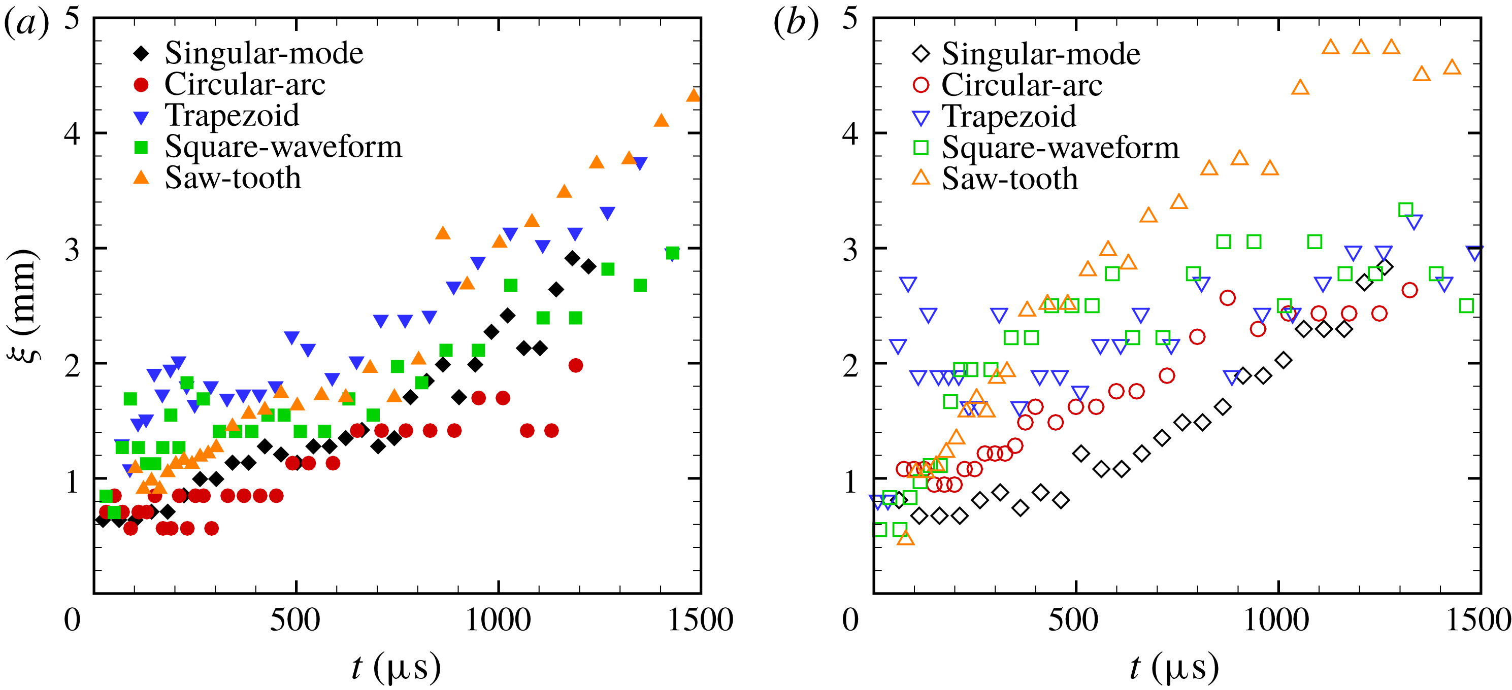
The thickness variation of the interface for small initial amplitude (a) and for high initial amplitude (b).

From the schlieren pictures, one can observe that the interface has a thickness. After the shock impact, the soap films become atomized. Due to the lower energy deposited by the shock wave on the soap film droplets in this work, the atomization is less efficient. The mean radius of the droplets is about $59~\unicode[STIX]{x03BC}\text{m}$ with the shock Mach number of 1.2 according to the work of Ranjan et al. (Reference Ranjan, Niederhaus, Oakley, Anderson and Bonazza2009). In addition, after the shock impact, the soap film is broken, and the gases at both sides diffuse quickly, forming an interface with a thickness. The interface thickness evolution is shown in figure 6 for each case. From the comparison, the interface appears significantly thicker in trapezoid, square-waveform and saw-tooth interface images. Several reasons may account for this change. Firstly, the thin pins used at each vertex to avoid the pressure singularity in these three interfaces will enhance the mixing near the vertexes (Prasad et al. Reference Prasad, Rasheed, Kumar and Sturtevant2000), resulting in a thicker interface. Secondly, the thin pins will somewhat impede the interface movement and increase its thickness. Thirdly, for these three interfaces, the initial interface height is 7.0 mm. However, for the single-mode and circular-arc interfaces, the actual initial interface height is 6.4 mm, as described above. More soap film droplets may result in a thicker interface. As the interface develops, the initially invisible small perturbations on the interface will also develop. Although these small perturbations have limited effects on the interface morphology, their development will increase the interface thickness. As a result, the interface thickness grows gradually for all cases.

4 Amplitude growth in the linear stage

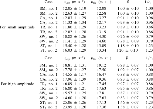
The experimental linear growth rates of different interfaces ( $v_{exp}$ ) are obtained by linear fitting of the experimental data before the growth rate reduces. For single-mode interfaces, the previous work (Niederhaus & Jacobs Reference Niederhaus and Jacobs2003; Liu et al. Reference Liu, Liang, Ding, Liu and Luo2018) indicated that the impulsive model (Richtmyer Reference Richtmyer1960) can provide an accurate prediction of amplitude growth rate of the interface when $a_{i0}/\unicode[STIX]{x1D706}$ is sufficiently small ( ${\leqslant}0.05$ ). However, when $a_{i0}/\unicode[STIX]{x1D706}$ is larger than 0.05, its prediction gradually deviates from the experiment as $a_{i0}/\unicode[STIX]{x1D706}$ increases (Rikanati et al. Reference Rikanati, Oron, Sadot and Shvarts2003; Dell et al. Reference Dell, Pandian, Bhowmick, Swisher, Stanic, Stellingwerf and Abarzhi2017). Therefore, in order to give an accurate prediction for the single-mode interface in this study, because the initial $a_{i0}/\unicode[STIX]{x1D706}$ is larger than 0.05, the impulsive model is modified by multiplying by a reduction factor $R$ :

(4.1) $$\begin{eqnarray}\displaystyle v_{the}=R\,k\unicode[STIX]{x0394}vA^{+}a_{i0}^{+}, & & \displaystyle\end{eqnarray}$$

where $v_{the}$ is the theoretical amplitude growth rate predicted by the modified impulsive model and $a_{i0}^{+}=a_{i0}(1-\unicode[STIX]{x0394}v/v_{s})$ is the post-shock amplitude. In this work, for the case with small initial amplitude, $R$ is 0.9 which is approximately the theoretical value discussed by Buttler et al. (Reference Buttler, Oró, Preston, Mikaelian, Cherne, Hixson, Mariam, Morris, Stone and Terrones2012). However, for the case with high initial amplitude, $R$ is 0.32 which is much smaller than the theoretical value ( ${\sim}0.7$ ). The failure of the theory to predict the reduction factor for high initial amplitude is believed to be caused partially by ignorance of the secondary compressible effects. As $a_{i0}/\unicode[STIX]{x1D706}$ increases, secondary compressible effects (shocks reflected from the upper and lower initial interfaces as well as the walls) become stronger and more vorticity is deposited on the interface, resulting in the suppressed linear growth rate of the interface and the earlier appearance of nonlinear growth of the interface perturbation (McFarland et al. Reference McFarland, Greenough and Ranjan2013). Based on the reduction factor $R$ , both $v_{exp}$ and $v_{the}$ are listed in table 3 for all cases. Note that because the modified impulsive model can predict the single-mode interface evolution well, to highlight the deviation degree of the quasi-single-mode interface from the single-mode one, $a_{i0}$ is still adopted in the theoretical prediction of the linear growth rate for all the quasi-single-mode interfaces. A ratio $\tilde{v}$ , defined as $\tilde{v}=v_{exp}/v_{the}$ , is also given in table 3 for each case. 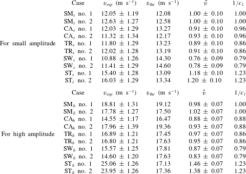In fact, $\tilde{v}$ represents the deviation degree of the quasi-single-mode interface from the single-mode one. As the initial interface gradually deviates from the single-mode one, the discrepancy between the prediction and the experiment is amplified. Specifically, the model underestimates the growth rate of the saw-tooth interface, while overestimating the growth rate of the other three interfaces.

To illustrate the role of the fundamental mode in the linear stage, $1/c_{1}$ , with $c_{1}$ being the coefficient of the fundamental mode in (2.1), is calculated and listed in table 3 for each case. The comparison of $1/c_{1}$ with $\tilde{v}$ indicates that although the initial interface deviates from the single-mode one, the fundamental mode of the initial interface determines the linear growth rate in all cases because the fundamental mode is dominant, and the effects of high-order modes can be ignored in the linear stage.

Table 3.

Comparison of linear growth rate of different cases: $v_{exp}$ is the experimental velocity obtained through linear fitting, $v_{the}$ is the theoretical velocity calculated by the incompressible theory of Richtmyer (Reference Richtmyer1960) and $\tilde{v}=v_{exp}/v_{the}$ ; $c_{1}$ is the coefficient of the fundamental mode in the Fourier expansion.

5 Amplitude growth in the nonlinear stage

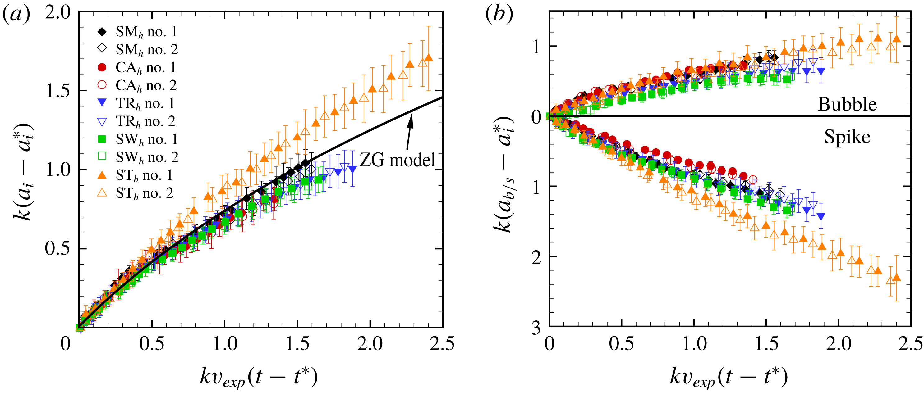
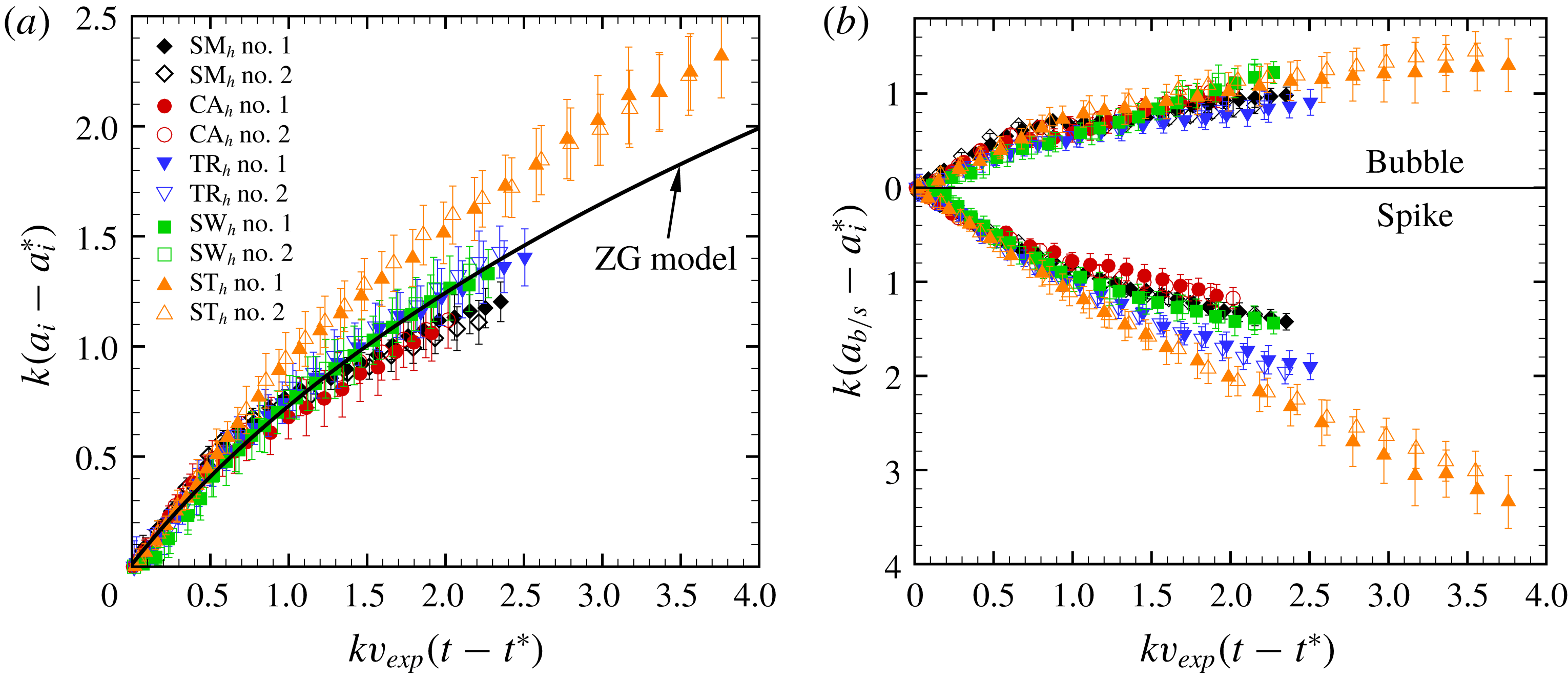
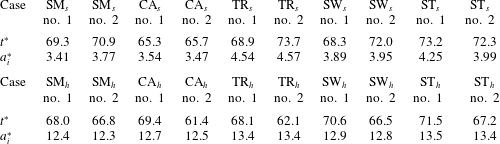
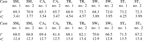
The amplitude growth as well as the evolutions of the spike and bubble are considered as shown in figures 7 and 8, respectively, for the small and high initial amplitude cases. The time is normalized by $kv_{exp}$ ( $t-t^{\ast }$ ) with $t^{\ast }$ being the characteristic time for the startup phase. According to Lombardini & Pullin (Reference Lombardini and Pullin2009), $t^{\ast }$ can be calculated by the following expression:

(5.1) $$\begin{eqnarray}\displaystyle t^{\ast }=\frac{1}{2k}\left(\frac{1-A^{+}}{v_{f}+\unicode[STIX]{x0394}v}+\frac{1+A^{+}}{v_{t}-\unicode[STIX]{x0394}v}\right), & & \displaystyle\end{eqnarray}$$

where $v_{f}$ and $v_{t}$ are the velocities of the reflected shock and transmitted shock, respectively. The amplitude is scaled as $k$ ( $a_{i}-a_{i}^{\ast }$ ) where $a_{i}^{\ast }$ is the corresponding experimental amplitude at $t^{\ast }$ . For all cases, the values of $t^{\ast }$ and $a_{i}^{\ast }$ calculated from (5.1) are provided in table 4. In experiments, the centre of the material layer, defined as the average position of the two boundaries, is considered as the interface boundary, and the error bars result from the thickness of the material layer. The dimensionless amplitude for different interfaces at the initial time is scaled at one point and the linear stage of perturbation growth is normalized. For the cases with small initial amplitude, as shown in figure 7(a), it can be found that the saw-tooth interface has the largest amplitude in the nonlinear stage (after dimensionless time about 0.5), while the other three quasi-single-mode interfaces have a smaller amplitude than the single-mode interface. This can be explained by their Fourier expansions. Compared with the single-mode interface, all the initial high-order modes in the saw-tooth interface have the same sign as the fundamental one and promote the perturbation growth, while the main high-order modes in the other three cases have an opposite sign to the fundamental one and inhibit the perturbation growth. However, for the cases with high initial amplitude, as shown in figure 8(a), the amplitude of the single-mode case seems relatively smaller than the quasi-single-mode interfaces. This amplitude reduction in the single-mode case is caused by the cavity formed at the spike head of the single-mode interface with high initial amplitude, as discussed before.

Figure 7.

Comparisons of the dimensionless amplitude of the interface (a) and of the bubble and spike (b) for all interfaces with small initial amplitude.

Table 4.

Values of $t^{\ast }$ and $a_{i}^{\ast }$ in all cases, and the units are $\unicode[STIX]{x03BC}\text{s}$ and mm, respectively.

Comparisons of the dimensionless spike width ( $a_{s}$ ) and the bubble width ( $a_{b}$ ) are presented in figures 7(b) and 8(b). The dimensionless $a_{s}$ of the saw-tooth interface is the largest among all cases because the curvature radius of the spike structure is infinitesimal. The dimensionless $a_{b}$ for all cases are quite close to each other and increase gradually. For the trapezoid and square-waveform interfaces with small initial amplitude, the dimensionless $a_{b}$ is almost unvaried after the dimensionless time of 1.2. At the late time evolution, as shown in figures 4(c) and 4(d), the curvature radius of the bubble head is almost infinite. According to the relationship between the amplitude $a_{i}$ and the curvature radius $R_{i}$ of the interface, $1/(kR_{i})=-\unicode[STIX]{x2202}^{2}a_{i}/\unicode[STIX]{x2202}x^{2}$ , the amplitude growth rate approaches zero when the the curvature radius is infinite.

Figure 8.

Comparisons of the dimensionless amplitude of the interface (a) and of the bubble and spike (b) for all interfaces with high initial amplitude.

The amplitude variations with time for the five cases are further compared with the prediction from the nonlinear model developed by Zhang & Guo (Reference Zhang and Guo2016) (ZG model). For the single-mode interface evolution, the ZG model is expressed as

(5.2) $$\begin{eqnarray}\displaystyle v(t)=\frac{v_{the}}{1+\hat{a}kv_{the}t}, & & \displaystyle\end{eqnarray}$$

where

(5.3) $$\begin{eqnarray}\displaystyle \hat{a}=\frac{3}{4}\frac{(1+A^{+})(3+A^{+})}{[3+A^{+}+\sqrt{2}(1+A^{+})^{1/2}]}\frac{[4(3+A^{+})+\sqrt{2}(9+A^{+})(1+A^{+})^{1/2}]}{[(3+A^{+})^{2}+2\sqrt{2}(3-A^{+})(1+A^{+})^{1/2}]}, & & \displaystyle\end{eqnarray}$$

with the positive Atwood number for bubbles and its negative counterpart for spikes with the same density ratio and $v(t)$ the growth rate at time $t$ . As shown in figure 7(a) for the interfaces with small initial amplitude, the ZG model gives a good prediction for the evolution of the single-mode interface. However, the model slightly overestimates the growth of the circular-arc, trapezoid and square-waveform interfaces. A worse prediction of growth is observed for the saw-tooth interface because of the existence of a kink- singularity which will accelerate the spike growth. The failure of the model in predicting the behaviour of the quasi-single-mode interfaces indicates that it is necessary to evaluate the effect of initial high-order modes on the perturbation growth in the weakly nonlinear stage. For the interfaces with high initial amplitude, as shown in figure 8(a), the ZG model overestimates the growth of the single-mode interface in the nonlinear stage due to the formation of the cavity that reduces the amplitude. As a result, the failure of the model at late stages is caused partially by the secondary compressible effect. Occasionally, the ZG model works well for the trapezoid and square-waveform interfaces. One possible reason is that the effects of initial high-order modes increase when the initial amplitude is large, and significantly change the growth rate.

For a single-mode interface, as the interface evolves, the fundamental mode will generate high harmonics. Zhang & Sohn (Reference Zhang and Sohn1997) proposed a model (ZS model) previously to predict the amplitudes of the first four harmonics. For a multi-mode interface, except for the fundamental mode, the high-order modes also exist on the initial interface. For an initially periodic interface, only odd-order modes exist on the initial interface. The even harmonics are generated as the interface develops from the initial odd-order modes and the coupling among them. Taking the first three harmonics in the present work for example, the fundamental and third modes exist on the initial interface. As the interface develops, the fundamental mode will generate the second and third harmonics. If mode coupling is considered, the coupling between the initial fundamental and third modes will also generate the second harmonic (Vandenboomgaerde et al. Reference Vandenboomgaerde, Gauthier and Mügler2002; Di Stefano et al. Reference Di Stefano, Malamud, Kuranz, Klein and Drake2015). To highlight the effects of high-order modes on amplitude growth, a Fourier analysis is performed here. Benefiting from the current method of interface formation, the high-quality schlieren pictures facilitate an accurate extraction of the interface contours with a simple image-processing program according to previous work (Liu et al. 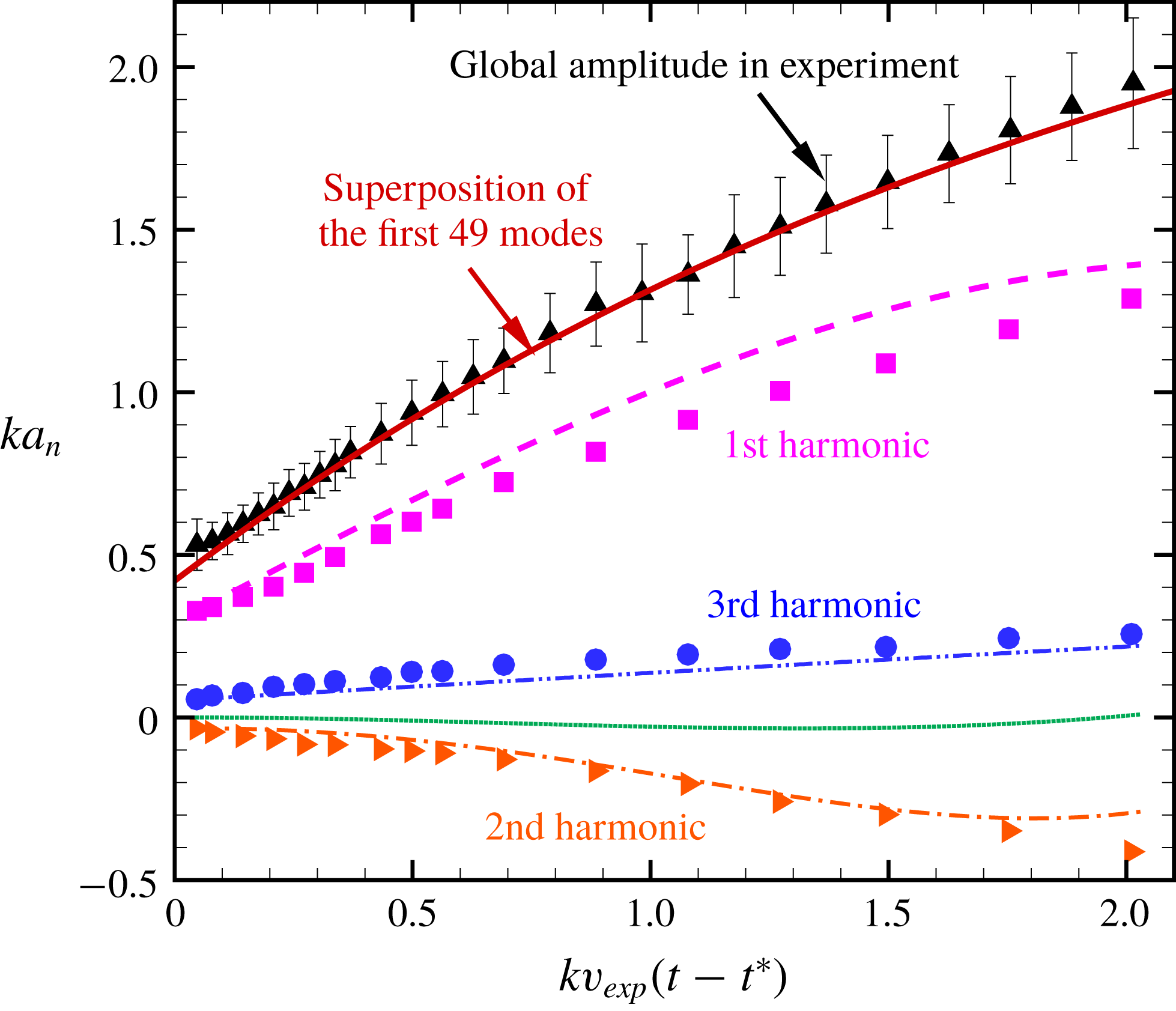Reference Liu, Liang, Ding, Liu and Luo2018). For the saw-tooth interface with small amplitude before the appearance of vortices, the amplitude growths of the first three harmonics are obtained from the experiment, as shown in figure 9. The amplitudes of the other higher harmonics from the experiment are neglected because they are quite small, and the errors are significant. For the first and second harmonics, the predictions from the ZS model are also given for comparison. The amplitude of the second harmonic in the experiment can be well predicted by the ZS model, which indicates that the second harmonic is generated only from the fundamental mode, and the coupling among initial fundamental and third modes is absent or weak enough that can be ignored during the time studied. For the third harmonic, except for the one initially existing on the interface, the one generated from the fundamental mode also contributes to the amplitude growth. For the amplitude of the third harmonic generated from the fundamental mode, the prediction from the ZS model shows that it maintains a very small value throughout the experiment duration, confirming the previous viewpoint (Liu et al. Reference Liu, Liang, Ding, Liu and Luo2018) for the single-mode interface. The expression which was proposed to predict the amplitude of the first mode in the ZS model is also adopted to predict the amplitude of the initial third mode with the corresponding frequency, the initial amplitude $a_{i0}^{+}\,c_{3}$ and initial velocity $v_{exp}\,c_{3}$ with $c_{3}$ being the coefficient of the initial third mode in (2.1). Figure 9 shows that the prediction of the initial third mode from the ZS model coincides well with the experimental result. This fact also indicates that the initial odd-order modes develop independently, which agrees with the statement by Mikaelian (Reference Mikaelian2005) that each mode will grow linearly and independently at early times before mode coupling becomes significant.

Figure 9.

Perturbation amplitude variation of the first three harmonics for the saw-tooth interface with small initial amplitude. The symbols represent the experimental results. The dashed, dash-dot and dotted lines represent the predictions of the first, second and third harmonics from the ZS model, respectively. The dash-dot-dot line represents the prediction of the initial third mode from the ZS model.

In figure 9, the global amplitude evolution from the experiment for the saw-tooth interface is also presented. Through comparison, one can find that the fundamental mode plays a dominant role in the amplitude growth. As the interface evolves, the discrepancy between the amplitude of the fundamental mode and the global amplitude is amplified, which means that the effects of the high-order modes on the amplitude growth must be considered. To predict the amplitude growth in the weakly nonlinear stage of the quasi-single-mode interface, the ZG model initially proposed for the single-mode interface is modified by considering the effects of high-order modes according to the linear superposition principle proposed by Mikaelian (Reference Mikaelian2005). The modified model (mZG model) can be expressed as

(5.4) $$\begin{eqnarray}\displaystyle v=\mathop{\sum }_{n}\frac{c_{2n-1}v_{the}/c_{1}}{1+(2n-1)\hat{a}kc_{2n-1}v_{the}/c_{1}t},\quad n=1,2,3,\ldots . & & \displaystyle\end{eqnarray}$$

Based on this model, the growth rate of each initial high-order mode can be obtained, and their linear superposition can result in the final growth rate of the quasi-single-mode interface. The predictions by the mZG model for the four quasi-single-mode interfaces with small and high initial amplitudes are presented in figure 10. In the present study, we choose to superimpose the smallest number modes to predict the experimental data until the prediction matches the experimental result (generally the difference between the prediction and the experiment is less than 3 %). For the cases with small initial amplitude, the superposition of the first three modes can give a reasonable prediction of the amplitude in experiment for the circular-arc interface, while a good prediction is only achieved for the saw-tooth interface after summing the first 49 modes. For the saw-tooth interface where only negative terms exist, adding more modes will not substantially alter the results after the prediction matches the experiment, i.e. the superposition over the modes converges asymptotically. For the interfaces where both positive and negative terms exist, after the prediction matches the experiment, adding more modes will alter the prediction, especially for the modes with relatively large coefficients. However, as the order of the mode increases, its coefficient becomes smaller and the effect on the prediction is gradually weakened. In other words, the superposition over the modes also converges but in an oscillatory way. For the cases with high initial amplitude, generally, superimposing more modes is needed to match the experiment, because the effects of high-order modes are significant as $a_{i0}/\unicode[STIX]{x1D706}$ increases. More high-order modes needed in the model to match the experiment illustrates more severe deviation of the interface from the single-mode one. Although the ZG model fails to predict the amplitude of the single-mode interface with high initial amplitude at nonlinear stages, the superposition over the modes can still provide a satisfactory prediction of the experiment amplitude for the quasi-single-mode interfaces. For the square-waveform interface with high initial amplitude, note that the modelled growth rate does not start from the origin. The startup time in the experiment is so long ( ${\sim}200~\unicode[STIX]{x03BC}\text{s}$ ) that equation (5.1) in invalid (the prediction is ${\sim}70~\unicode[STIX]{x03BC}\text{s}$ ), probably due to the complicated wave patterns in the square-waveform interface. As a result, the amplitude is predicted when the interface enters the linear phase in the experiment. The mZG model provides a satisfactory prediction of the experiments, which verifies that the coupling among different initial modes can be ignored when the fundamental mode is dominant as is the case in this work, especially for the small initial amplitude.

Figure 10.

Comparison of the dimensionless amplitude in experiments with the prediction from the modified ZG model for the quasi-single-mode interfaces. Circular-arc (a), trapezoid (b), square-waveform (c) and saw-tooth (d).