

Introduction
In contrast to pre-modern, tribal and rural societies, where male status and wealth are generally converted into higher reproductive success, in modern societies the association between socioeconomic status and reproductive output has usually been reported null or negative. Positive associations among male status, resources and reproduction have been demonstrated in a wide range of traditional hunter-gatherer, rural and agricultural societies (the Turkmen pastoralist: Irons, Reference Irons, Chagnon and Irons1979; the Kipsigis: Borgerhoff Mulder, Reference Borgerhoff Mulder and Clutton-Brock1988; the Yanomano: Chagnon, Reference Chagnon1988) as well as in some pre-industrial societies (Mealey, Reference Mealey1985; Voland, Reference Voland1990). In modern societies, people seem to voluntarily reduce their levels of fertility, especially in families of higher socioeconomic status. These findings pose a major challenge to scientific fields as diverse as evolutionary anthropology, demography and economics (e.g. Vining, Reference Vining1986). Nevertheless, in one very important respect these generalizations are overstated: the data on which they are based represent offspring counts mainly for women, not for men. In modern demography, the offspring count of men is very rarely sampled in censuses and other surveys. Thus conclusions regarding how socioeconomic status influences reproductive output typically rely solely on female data, where the association between status or wealth and reproduction is negative (for reviews see Barrett et al., Reference Barrett, Dunbar and Lycett2001; Skirbekk, Reference Skirbekk2008).
Early results along the line of these refinements are strikingly counterintuitive. When men and women in modern societies are analysed separately by offspring count as well as by socioeconomic status, a positive association emerges between male socioeconomic status and reproduction but not between female status and reproduction (Fieder et al., Reference Fieder, Huber, Bookstein, Iber, Schäfer, Winckler and Wallner2005; Hopcroft, Reference Hopcroft2006; Weeden et al., Reference Weeden, Abrams, Green and Sabini2006; Fieder & Huber, Reference Fieder and Huber2007; Nettle & Pollet, Reference Nettle and Pollet2008). Fieder & Huber (Reference Fieder and Huber2007) (data from modern Sweden) and Nettle & Pollet (Reference Nettle and Pollet2008) (data from contemporary United Kingdom) report a positive relationship between male income and offspring count. They attribute this finding mainly to the higher percentage of childlessness among men of low income, which may in turn be the result of the low-income male's higher probability of remaining unmarried (Fieder & Huber, Reference Fieder and Huber2007). This view is consistent with marriage patterns reported so far, showing that a greater fraction of lower-income men as well as unskilled men remain unmarried or without a partner (Forsberg & Tullberg, Reference Forsberg and Tullberg1995; Nakosteen & Zimmer, Reference Nakosteen and Zimmer1997; Burgess et al., Reference Burgess, Propper and Aassve2003). It has been suggested that the association between income and marriage rate in men might be an expression of the evolutionary phenomenon that Darwin named sexual selection. In this interpretation, females prefer, or at least should prefer, men of high socioeconomic status as mates because such men offer more resources, protection and earning potential than those of lower status (Buss & Barnes Reference Buss and Barnes1986; Buss, Reference Buss1999). Consequently, men of higher socioeconomic status should have higher access to reproductive women, who, in turn, should adjust their reproductive decisions accordingly. The result should be a positive association between male socioeconomic status and reproductive success, whether demonstrated in pre-modern or in modern societies.
The present paper examines associations linking chances of marrying or reproducing to income and education using census data from six different countries. As reproductive strategies and marital patterns differ between the sexes (Fieder & Huber, Reference Fieder and Huber2007; Mamum, Reference Mamum2008; Nettle & Pollet, Reference Nettle and Pollet2008), each analysis is performed separately for men and women. In modern censuses, data on the number of offspring are at best sampled for women only, whereas often data on the number of one's own children in the household are available for both sexes. With the following study it is intended to confirm the results on income and childlessness in men on the basis of data from censuses from different countries. As marital status itself is typically available for both men and women, the available data thus facilitate the analysis of the following questions:
1. Is income or educational attainment associated with the probability of remaining unmarried?
2. Is the frequency of childlessness associated with income and educational attainment?
3. Do these associations differ between men and women?
Of course living without children in the same household is an imperfect proxy of childlessness that may be affected as much by confounding factors such as sex and age as by a man's income and education. Also, the association between income and marriage may be bidirectional: in men, for instance, high income may increase the chance of marrying, but marriage may also lead to higher income (Mamum, Reference Mamum2008). Still, there is great value in the truly enormous samples (here, a total of nearly 10 million records) that were made available by contemporary governments in the form of their own censuses.
Methods
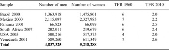
Census data from six countries are used as provided by IPUMS International (Minnesota Population Center, Integrated Public Use Microdata Series, International, Version 6.0 [Machine-readable database], University of Minnesota, Minneapolis, 2010): Brazil, Mexico, Panama, South Africa, USA and Venezuela. Despite pronounced differences in economic development all six countries underwent a significant fertility drop from 1960 to 2010, i.e. showing a modern pattern concerning fertility (Table 1). These are all the IPUMS-distributed censuses from the current century that offer information on marital status, age, childlessness, education and income. Marital status is coded in the raw IPUMS records as single/never-married, married/in union, separated/divorced/spouse absent, widowed, cohabitation. This variable was recorded into a simple binary contrast: ever-married versus never-married. Age is in years at the time of the census. The estimate of childlessness was, operationally, a dichotomization of the number of one's own children in the household: zero versus one or more. The same variable had to be used for both men and women in the samples, as this count was not separately by marital partner. Educational attainment is categorized as follows: E1, less than primary completed; E2, primary completed; E3, secondary completed; E4, university completed. As the probability of marriage, having children, and income are strongly age dependent, plots compare rates of marriage and childlessness age by age. Regressions are pooled over ages but always incorporate a term for a (linear) age effect.
The study sample by country and sex, as well as total fertility rate (TFR), for each country in 1960 (World Bank) and 2010 (World Population Data Sheet 2010)

Income was coded as follows: for Brazil 2000, USA 2005, South Africa 2007 and Venezuela 2001, the total income of a person from all sources in the previous year was used. For Panama 2001, monthly wage and salary income, the only income information IPUMS offers from this census, was used. For the purpose of some of the country-specific analyses below, income for each census, each sex, and each year of age was divided into four quartiles labelled Q1 to Q4, except in Mexico where, owing to particularly severe truncation of the raw data, there are only three ‘quartiles’. In the regressions, for distributional reasons income was entered in the form of the square root (see also Huber et al., Reference Huber, Bookstein and Fieder2010).
There is a risk in using the variable ‘no own children in the household’ as an estimate of childlessness, particularly in men. For instance, after divorce or separation, children typically remain in their mother’s rather than the father’s household. However, owing to the fact that the number of children is sometimes not even sampled for women and almost never sampled for men by regular censuses, this variable is the only possibility if any estimate of childlessness for both sexes across countries and cultures is to be analysed.
The most recent data sets offered by IPUMS were used: Brazil 2000, Mexico 2000, Panama 2001, USA 2005, South Africa 2007, USA 2005 and Venezuela 2001. Only men and women in ‘their reproductive years’, from the age of 16 to the age of 50 years, were included. For Brazil 2000, USA 2005 and South Africa 2007, the data of the ethnic majority were analysed (Brazil 2005: Whites; USA 2005: Whites; South Africa 2007: Black Africans). For Mexico 2000 and Panama 2001, which offer no further information on ethnicity, all individuals of indigenous origin were excluded. For Venezuela 2001, IPUMS provides no information on ethnicity, so all individuals within the appropriate age range were included. The samples totalled 4,837,325 men and 5,218,288 women (Table 1).
For each integer age between 16 and 50 the sample fraction of individuals who had never been married and the sample fraction who live without any of their own children in the household were re-plotted. These plots are separate by sex and by income quartile and for each education category as well. Also, separately by sex and country, logistic regressions of binary marital status were calculated (0=never married, single; 1=married at some point) on income, categorized educational attainment and age. Separately by sex and country, logistic regressions were also calculated of the binary proxy for childlessness (0=no child in household; 1=child(ren) in household) on income, categorized educational attainment and age. As the relation between age and marital status as well as childlessness is not linear, a quadratic term for age was included in all logistic models for the never-married variable.
Null-hypothesis statistical significance levels were not reported owing to the very large sample size (Ziliak & McCloskey, Reference Ziliak and McCloskey2008).
Results
For both men and women, the proportion of never-married individuals as well as those without own children in the household rapidly decreases with age through the middle 30s and remains low. The proportion of individuals without children in the household similarly decreases through the middle 30s but in some samples the trend reverses at about age 40, perhaps because children start leaving the parental household.
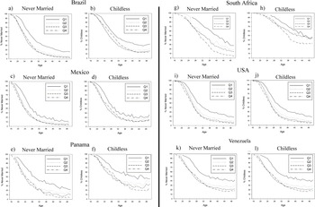
Figure 1 presents the statistics of marital status and childlessness by age and income quartile. Within the men of each national sample, at almost every age the percentage of never-married individuals is highest in the lowest income quartile, and when the highest three quartiles differ in percentage never-married, the differences are nearly always concordant with the income sort. Likewise at almost every age, the percentage of childless individuals is highest in the lowest income quartile, but the differences are less pronounced among the quartiles above that.
a, c, e, g, i, k: percentage of never-married men for each income quartile – Q1 (lowest), Q2, Q3 and Q4 (highest) – separately by census. b, d, f, h, j, l: percentage of men without own children in the household for each income quartile separately for each census.

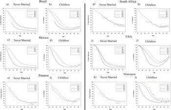
In women, the pattern is the reverse (Fig. 2). The highest percentage of never-married women is found in the highest income quartile: Q4 in Brazil, Panama, Venezuela and US and Q3 in Mexico. In the US, differences among income quartiles above the lowest are small, and in South Africa there seems to be little effect of income on marital status at all. The percentage of childless women by income quartile resembles the pattern for proportion never-married. For this outcome, the effect of income quartile appears to be more pronounced, even in South Africa and the US.
Percentage of never-married women and women without own children in household for each income quartile, coded as in Fig. 1.

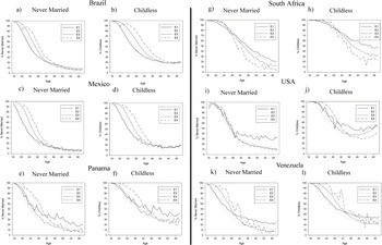
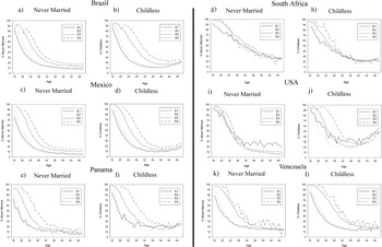
The association between educational attainment and marital status in men shows a more subtle picture (Fig. 3). In Brazil and Mexico, the highest proportions of never-married men are found in the highest educational category and the lowest proportions in the lowest two educational categories. But in South Africa, except at the youngest ages, the proportion of never-married men is lowest in the highest educational category and highest in the lowest educational category. In both Panama and Venezuela, a higher proportion of young men are unmarried among the highest educational category, whereas among the older men it is those of the lowest educational category who more often have never married. These reversals suggest either a different distribution of ages at first marriage or historically contingent cohort effects (see Discussion). In the US, with increasing age the percentage of unmarried men increases in the lowest educational category. The association between educational attainment and the proxy for childlessness is similar to that between marital status and educational attainment except for the US, where the curves are more widely spread at younger ages.
a, c, e, g, i, k: percentage of never-married men for each education category – E1 (lowest), E2, E3, E4 (highest) – separately by census. b, d, f, h, j, l: percentage of men without own children in the household for each education category separately for each census.

In women, the association between educational attainment and marital status is likewise more complex than that for income, and sometimes it is concordant rather than discordant with the association seen for men (Fig. 4). In Brazil, Mexico, Panama and Venezuela, the highest proportions of unmarried women are found in the highest educational category and the lowest proportions in the lower two educational categories. In South Africa, no apparent relationship between marital status and educational level is observable. In the US, as for men, there is no apparent association between education and dichotomized marital status at young ages, but later the proportion of unmarried women increases in the lowest educational category. In women, the association between educational attainment and the childlessness proxy again is similar to that for marital status, except for the US and South Africa, where the curves are more widely spread at younger ages.
Percentage of never-married women and women without own children in household for each education category, coded as in Fig. 3.

The logistic regressions correspond to the preceding figures: regressions of dichotomous marital status or dichotomous childlessness on square root of income and on educational category. In every subsample of men, having been married is positively related to income, but the relationship between educational category and marital status is not even consistent in sign across census samples (Table 2). In the female subsamples, having been married is always negatively associated with income except for South Africa, and, again, the relationship with education is unstable (Table 3). In all samples, having at least one own child in the household in men is positively related to income, whereas the relationship between educational category and not being childless is not consistent in sign across census samples (Table 4). In the female subsamples, having at least one own child in the household is always negatively associated with income, and the relationship to education is again less stable (Table 5). These findings confirm the reversal of the income–marital status association between the sexes in this wide range of contemporary societies, a consistency that does not obtain for the seemingly analogous association with education.
Logistic regression of income and age, and educational attainment and age, on marital status (encoded as 0=never married, 1=ever married) in men aged between 16 and 50 years for each census
a Reference: university completed.
Logistic regression of income and age, and educational attainment and age, on marital status (encoded as 0=never married, 1=ever married) in women aged between 16 and 50 years for each census
a Reference: university completed.
Logistic regression of income and age, and educational attainment and age, on the proxy for childlessness (0=no own child in household, 1=at least one own child in household) in men aged between 16 and 50 years for each census
a Reference: university completed.
Logistic regression of income and age, and educational attainment and age, on the proxy for childlessness (0=no own child in household, 1=at least one own child in household) in women aged between 16 and 50 years for each census
a Reference: university completed.
Discussion
The findings, on the basis of census data from six countries, confirm results found on the basis of Swedish data (Fieder & Huber, Reference Fieder and Huber2007) and data from Great Britain (Nettle & Pollet, Reference Nettle and Pollet2008) and gives the results found earlier further cross-national validation. The predictions from income are consistent and strongly contrasting by sex, whereas the forecasts from education are inconsistent over country in men, and generally stronger for women than men. Particularly highly educated women have a higher chance of childlessness at all ages than less well educated women. In principle there should be some sort of interchangeability between income and education, as both represent invested human capital, both make adult life far more comfortable and meaningful, both are subject to assortative mating, and both contribute to some underlying general factor of ‘socioeconomic status’ in most modern societies. Yet evidently, in spite of their well known correlation in all modern societies, they contribute differently and in fact paradoxically to trends in this study’s dichotomized marital status measure and proxy for childlessness.
The results should not be over interpreted. While the signs of the logistic regression coefficients for income are consistent in Table 2, the magnitudes vary by a factor of more than ten in either sex. The association between education and marital status, as well as the estimate of childlessness, is nuanced in the data analysed, perhaps as a combination of secular effects along with institutional aspects of the educational system country by country.
On the other hand, the consistency of the opposite association between income and marital status in men and women of all six countries, despite their different economic levels, is striking and may emphasize a ‘universal significance’ of different effect of income for men and women in relation to marriage and reproduction. A consistent maximum for never-married status and for childless status is found in the lowest quartile of income for males, regardless of country, contrasted with the same maximum for the highest quartile of income for females. A preference for men of high status and income can be found across cultures (Buss, Reference Buss1999) and has been shown to pay off in reproductive terms, as Huber et al. (Reference Huber, Bookstein and Fieder2010) found that a woman’s probability of remaining childless decreases with increasing husband’s income, whereas among the higher educated women, husband’s income was positively associated with a woman’s offspring count. These findings in a modern society might also be regarded as a hint to an ongoing selection of humans along ‘cultural traits’ (Stearns et al., Reference Stearns, Byars, Govindaraju and Ewbank2010).
The relationship between marriage and income has been widely discussed, particularly for men. The data are consistent with either or both of two causal paths: men of high income might be likelier to marry, but also the very state of marriage might somehow induce in men the conditions leading to a higher income (i.e. spousal pressure). Mamum (Reference Mamum2008) presented a review of the most recent findings on the topic: a rise in wage rates and hours worked increases a man’s likelihood of marriage and in turn marriage increases working hours and wage rates (Ahituv & Lerman, Reference Ahituv and Lerman2007); higher earnings have a positive association with the likelihood of marriage for men but a negative association in women (Burgess et al., Reference Burgess, Propper and Aassve2003); and earning potential is positively associated with the likelihood of marriage for men but not for women, but has no significant effect on cohabitation (Xie et al., Reference Xie, Raymo, Goyette and Thornton2003). Both a better female labour market and a worse male labour market are negatively associated with marriage rates in white women (Blau et al., Reference Blau, Kahn and Waldfogel2000). In addition, employment and earnings are positively associated with the likelihood of marriage in men (Mamum, Reference Mamum2008). This is also consistent with the pattern found by Fieder & Huber (Reference Fieder and Huber2007) on the basis of Swedish data.
Failure to report ever having married does not necessarily mean that the person has not formed a lasting relationship. So differences in cultural norms with respect to marriage in the examined countries could have affected the interpretation of the results. Except for the US (8.2%; Ambert, Reference Ambert2005) and Mexico (18.5%; Ambert, Reference Ambert2005), however, no data were available on the extent of cohabitation in these countries. Yet, according to Smock (Reference Smock2000), partner choice patterns are not substantially different between cohabiting and married couples. In addition, at least in Europe, marriage and cohabitation become even more similar as cohabitation becomes more common in society (Hamplova, Reference Hamplova2009). Inclusion of cohabitation is therefore not likely to change the conclusions considerably.
It is rational for a woman married to a man of higher income to be likelier to have children, and it is rational for the woman herself having a higher income to have fewer children. However, there is positive assortative mating by income (and education); hence these trends pull in opposite direction. It is difficult to construct a rationale for the consistency of the sign of the income effect across country within sex that would not at the same time argue against the meaningfulness of any difference in sign between the sexes. An explanation in terms of differences in assortative mating patterns by country would have to explain why those patterns were different between income and education. In addition, any understanding of the impact of income and education on fertility in modern societies will need to consider the sexes separately: this study’s two principal predictor variables – income and education – evidently have different meanings by sex.
Acknowledgment
The authors thank the anonymous reviewer for the valuable comments. For providing the census data, they thank: the Minnesota Population Center, Integrated Public Use Microdata Series, International, Version 6.0 (Machine-readable database), University of Minnesota, Minneapolis, 2010. Brazil: Institute of Geography and Statistics; Mexico: National Institute of Statistics, Geography, and Informatics; Panama: Census and Statistics Directorate; South Africa: Statistics South Africa; United States: Bureau of the Census; Venezuela: National Institute of Statistics.